Embed Size (px)
Citation preview

Thesis in Electrical Engineering Department of Electrical Engineering, Linköping University, 2016
Investigating Validation of a Simulation Model for Development and Certification of Future Fighter Aircraft Fuel Systems
Isac Strömberg and Markus Vilhelmsson

Division of Automatic Control
Department of Electrical Engineering
Linköping University SE-581 83 Linköping, Sweden
Copyright 2016 Isac Strömberg and Markus Vilhelmsson
Thesis in Electrical Engineering
Investigating Validation of a Simulation Model for Development and
Certification of Future Fighter Aircraft Fuel Systems
Isac Strömberg and Markus Vilhelmsson
LiTH-ISY-EX--16/4974--SE
Supervisors:
Fredrik Carlsson
SAAB AB
Du Ho
ISY, Linköping University
Examiner:
Johan Löfberg
ISY, Linköping University

ii
ABSTRACT
In this thesis a method for verification, validation and uncertainty quantification (VV&UQ) has been tested
and evaluated on a fuel transfer application in the fuel rig currently used at Saab. A simplified model has been
developed for the limited part of the fuel system in the rig that is affected in the transfer, and VV&UQ has
been performed on this model. The scope for the thesis has been to investigate if and how simulation models
can be used for certification of the fuel system in a fighter aircraft.
The VV&UQ-analysis was performed with the limitation that no probability distributions for uncertainties
were considered. Instead, all uncertainties were described using intervals (so called epistemic uncertainties).
Simulations were performed on five different operating points in terms of fuel flow to the engine with five
different initial conditions for each, resulting in 25 different operating modes. For each of the 25 cases, the
VV&UQ resulted in a minimum and maximum limit for how much fuel that could be transferred. 6 cases were
chosen for validation measurements and the resulting amount of fuel transferred ended up between the
corresponding epistemic intervals.
Performing VV&UQ is a time demanding and computationally heavy task, which quickly grows as the model
becomes more complex. Our conclusion is that a pilot study is necessary, where time and costs are evaluated,
before choosing to use a simulation model and perform VV&UQ for certification. Further investigation of
different methods for increasing confidence in simulation models is also needed, for which VV&UQ is one
suitable option.
iii
ACKNOWLEDGMENTS
For 20 weeks we have been spending full time at the Division for Test, Flight and Verification (TFV) at Saab,
working on this master thesis. We would like to thank everyone there for making our stay a fun and exciting
last semester of our education. A special thanks to the Fuel Section for all assistance, and of course to our
supervisor Fredrik Carlsson that has given us the opportunity to carry out the thesis and has also helped out
continuously when needed. We would also like to thank the fuel modelling division (TDGT) for supporting us.
We would also like to thank our supervisor Du Ho at Linköping University, for support and feedback on the
report. Thanks to Johan Löfberg, who has been our examiner at Linköping University, for general support and
guidance during our work.
Lastly, we would like to say thanks to each other for a great cooperation throughout the thesis.
Linköping, May 2016
Isac Strömberg and Markus Vilhelmsson

iv
TABLE OF CONTENTS
1 Introduction ............................................................................................................................................... 1
1.1 Motivation ......................................................................................................................................... 1
1.2 Purpose .............................................................................................................................................. 2
1.3 Problem statements .......................................................................................................................... 2
1.4 Limitations ......................................................................................................................................... 2
1.5 Outline of the report ......................................................................................................................... 2
2 Theory ........................................................................................................................................................ 3
2.1 System overview ................................................................................................................................ 3
2.2 Creating a simulation model ............................................................................................................. 5
2.3 Verification, validation and uncertainty quantification (VV&UQ) ..................................................... 6
2.3.1 Uncertainty identification and characterization ....................................................................... 7
2.3.2 Verification process ................................................................................................................... 8
2.3.3 Validation process ..................................................................................................................... 9
2.3.4 Total uncertainty computation ................................................................................................ 10
2.4 Uncertainty quantification of aircraft systems ................................................................................ 11
2.5 Sampling for propagation of uncertainties...................................................................................... 13
2.6 Certification ..................................................................................................................................... 14
2.6.1 Type- and Airworthiness Certificate based on JAR 21/EASA 21 .............................................. 16
2.6.2 Type certification process ........................................................................................................ 17
2.6.3 Swedish military rules .............................................................................................................. 17
3 Method .................................................................................................................................................... 18
3.1 Define model requirements ............................................................................................................ 19
3.1.1 Intended use ............................................................................................................................ 19
3.1.2 Requirements .......................................................................................................................... 20
3.2 Develop model- and VV&UQ-plan ................................................................................................... 21
3.3 Develop model................................................................................................................................. 22
3.4 VV&UQ ............................................................................................................................................. 24
3.4.1 Numerical uncertainty ............................................................................................................. 24
3.4.2 Input and model form uncertainties ....................................................................................... 26
3.4.3 Approximate characterization and screening SA .................................................................... 28
3.4.4 Detailed characterization ........................................................................................................ 30
3.4.5 Minimum/maximum parameter settings ................................................................................ 30
3.4.6 Uncertainty propagation at top level ...................................................................................... 31
3.4.7 Validation and inter-/extrapolation of uncertainties .............................................................. 33

v
4 Results ..................................................................................................................................................... 35
4.1 Total uncertainty ............................................................................................................................. 35
4.2 Validity check of min/max parameter settings ............................................................................... 37
4.3 Validation ......................................................................................................................................... 39
5 Discussion ................................................................................................................................................ 40
5.1 Results ............................................................................................................................................. 40
5.2 Method ............................................................................................................................................ 41
5.3 Certification potential of simulation models ................................................................................... 43
6 Conclusions .............................................................................................................................................. 45
7 Further development .............................................................................................................................. 46
8 Bibliography ............................................................................................................................................. 47
Appendix A – Linearity in uncertainties wrt the SRQ ...................................................................................... 49
vi
LIST OF FIGURES
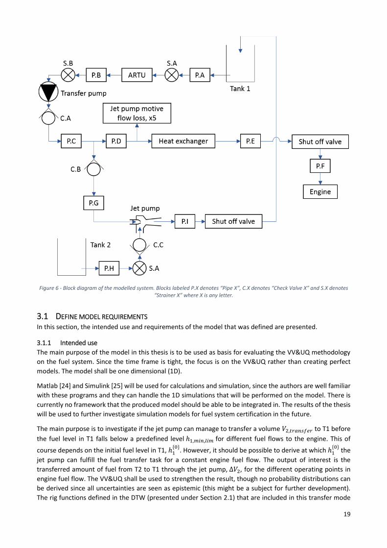
Figure 1 – Shows the components of the simplified fuel system (back-up mode). _______________________________ 3 Figure 2 - Simulation model development process at Saab _________________________________________________ 6 Figure 3 - Example of a probability box and how it is affected by adding uncertainty information [15] _____________ 10 Figure 4 - Probability box example from [14] ___________________________________________________________ 11 Figure 5 - An overview of the method used in this thesis. _________________________________________________ 18 Figure 6 - Block diagram of the modelled system. Blocks labeled P.X denotes “Pipe X”, C.X denotes “Check Valve X” and
S.X denotes “Strainer X” where X is any letter. __________________________________________________________ 19 Figure 7 – Simplified block diagram with measurement signals marked in red. ________________________________ 21 Figure 8 - Shows the transfer pump model. ____________________________________________________________ 22 Figure 9 - Shows the jet pump graph. _________________________________________________________________ 23 Figure 10 - Comparison of step length. ________________________________________________________________ 25 Figure 11 - Shows the simulation model with the uncertainties implemented. ________________________________ 28 Figure 12 - Shows how the SRQ varies when the uncertainty in V1 is varied. __________________________________ 32 Figure 13 - Shows how the SRQ varies when the uncertainty in V2 is varied. __________________________________ 32 Figure 14 - Shows how the SRQ varies when the uncertainty in h2 is varied. __________________________________ 33 Figure 15 - Shows the minimum and maximum transferred volumes after the VV&UQ-evaluation of the first case. __ 35 Figure 16 – Shows the minimum and maximum transferred volumes after the VV&UQ-evaluation of the second case. 36 Figure 17 - Shows the minimum and maximum output in the SRQ together with the minimum transfer limit for the
different operating modes, for first case with total transferred volume at each operating point. _________________ 37 Figure 18 - Shows the minimum and maximum output in the SRQ together with the minimum transfer limit for the
different operating modes, for second case with transferred volume at each operating point during 𝑡𝑠𝑖𝑚. _________ 38 Figure 19 - Shows the validation data, nominal simulation output and min/max output. ________________________ 39

vii
LIST OF TABLES
Table 1 - Requirements on the model. .............................................................................................................................. 20 Table 2 - Requirements on the VV&UQ. ............................................................................................................................ 20 Table 3 - Template for uncertainty presentation. ............................................................................................................. 24 Table 4 - Numerical uncertainties. .................................................................................................................................... 26 Table 5 - Input and model form uncertainties. ................................................................................................................. 27 Table 6 - Remaining uncertainties after SA for all operating points. ................................................................................ 29 Table 7 - Remaining uncertainties after SA, constant simulation time for all operating points. ...................................... 30

viii
LIST OF ABBREVIATIONS AND ACRONYMS
Abbreviation/ Acronym
Meaning Explanation
MBSE Model-Based System Engineering The use of modelling to support system requirements, design, analysis, verification and validation activities.
NGT Negative-G Tank A fuel tank that allows an aircraft to fly at negative gravity forces.
T1, T2 Tank 1 and 2 Fuel tanks in the aircraft.
GECU General Electronic Control Unit A control unit in the aircraft that controls different systems, like the fuel system.
VT Vent Tank A tank where the transfer pump is placed, no storage of fuel.
ARTU Aft Refueling/Transfer Unit A valve in the fuel system.
DTW Declaration of Test Worthiness A document describing the fuel rigs ability to test aircraft functionality.
DAE Differential Algebraic Equation Equation containing differential and algebraic equations.
V&V Verification and Validation Process for determining what a simulation model can/cannot do.
UQ Uncertainty Quantification Process for quantifying how uncertainties affects a simulation model.
VV&UQ Verification, Validation and Uncertainty Quantification.
UQ is especially considered during V&V.
SRQ System Response Quantity A quantity (pressure, etc.) of interest during UQ.
SA Sensitivity Analysis A method for determining the effect of change in input on SRQs.
CDF Cumulative Distribution Function Integrated probability density function.
MCS Monte Carlo Sampling Sampling algorithm.
LHS Latin Hypercube Sampling Sampling algorithm.
P-box Probability box A way of extending CDFs for UQ.
TC Type certificate A certificate of aircrafts, necessary to get a CofA.
CofA Certificate of airworthiness The certificate of an aircraft which authorizes it to fly.

1
1 INTRODUCTION
This chapter presents the motivation for the thesis, what the purpose and problem statements are and what
limitations that are made. The outline of the report is also presented.
1.1 MOTIVATION This thesis has been carried out at Saab Aeronautics in Linköping, Sweden. The fuel system of the current
fighter aircraft (JAS 39 Gripen) has been developed and tested by Saab using a physical test rig and the
assignment is to investigate if simulation models can be used instead in the future. In the industry today a
lot of testing is performed using physical test equipment. The problem with physical test equipment, such as
test rigs, is that they are expensive to build and often has limited functionality. Therefore interest exists to
go further towards Model-Based System Engineering (MBSE), to shorten development time and lower cost.
A vital step when creating and using simulation models is the validation, which shows if the model is a good
approximation of the real system. In traditional validation the predicted output is compared to
measurements from the physical system to be able to draw conclusions about the model quality. A problem
that appears when deciding to use models, instead of physical test rigs, as a tool for development and
requirement testing is that the physical system will not exist. When there is no physical system to compare
with, how can the model designer be certain that the developed model is good enough?
At Saab today, testing is done in both simulation and with physical test rigs. Requirements that the test results
are supposed to show compliance with are airworthiness requirements, functional requirements and
performance requirements. Airworthiness requirements is the type of requirements that if not fulfilled, the
aircraft will not be allowed to fly. These are the toughest requirements to prove that the aircraft systems can
handle, since they are of highest importance. Initial airworthiness must be reached before the aircraft flies
for the first time, which is done by combining experience with test results from models and rigs. When this
is achieved flight testing will be performed by flying carefully at first, then increasing the difficulty of
maneuvers and thereby increasing the flight envelope, i.e. the operating region. Functional requirements
are the type of requirements that can be answered by yes/no, and that is not crucial for flight. “Can the fuel
system transfer fuel to the collector tank during flight?” These requirements are easier to prove than the
airworthiness requirements. Today, these requirements are partially tested in test rigs and partially on
ground tests in the aircraft. Performance requirements are the “easiest” requirements to test. They can be
seen as added value for the customer. Requirements of this type can be; “how long can the aircraft fly at
maximum throttle?” Whether the result of this requirement is 400s or 500s does not have crucial impact on
the aircrafts ability to fly, it is of course better if the result is 500s rather than less but it will still be able to
fly. Today, simulation is used to answer several performance requirements at Saab. Efforts from Saab are
currently done to go towards testing of functional requirements with simulation models, and in this way
reduce the amount of rig testing.
Apart from a possible reduction in time and cost when replacing a test rig with simulation models, the
material consumption can be reduced which is beneficial for the environment. Saab employs a lot of people,
both internally and externally through sub-contractors and business partners. Their products are an
important part of the Swedish Armed Forces, and also for many other countries. Digitalization is highly
relevant for the future industry and it is important to keep up with this progress. The technically advanced
products that Saab develops impels research and puts Sweden in a leading position.

2
1.2 PURPOSE The purpose of this thesis is to investigate if a simulation model is an adequate tool to use as basis for
certification of the fuel system in a fighter aircraft. The investigation should include a comparison with the
fuel rig that is currently used today at Saab, along with theory regarding the certification procedure and how
to build confidence into a simulation model.
A simulation model on a downsized part of the fuel system will be created, either from existing models or
from scratch depending on what is currently available at Saab. A method for “Uncertainty Quantification”
(UQ) will be evaluated and performed on the simulation model.
1.3 PROBLEM STATEMENTS These problem statements will be answered in this thesis:
How is the fuel test rig used today, in terms of certification of fighter aircraft fuel systems?
Could parts of the purpose with the physical fuel rig be fulfilled with a simulation model? In that case,
which parts?
What is required of a simulation model for being able to certify aircraft fuel systems?
Can UQ be used for determining the reliability of a simulation model of the fuel system in fighter
aircrafts?
1.4 LIMITATIONS The model that will be produced and used for UQ will be a part of the total fuel system, the test case will be
a specific backup mode with specified operating points. The considered system (fuel rig) is standing still on
the ground. No account will be taken to gravity forces, center of gravity or such effects that would be
significant for a moving system. Only stationary flow will be considered and the fluid is seen as incompressible,
no dynamic experiments or simulations will be analyzed. The pressurization system for the fuel tanks will be
decoupled, which gives atmospheric pressure in the tanks. The uncertainties in model equations and inputs
will be considered solely epistemic, which means that no probability distributions will be considered.
1.5 OUTLINE OF THE REPORT Chapter 2 will present the theory on which the thesis is based. Firstly an overview of the system is given and
the basics of creating a simulation model will be presented. A comprehensive framework for verification,
validation and uncertainty quantification is then presented. From the comprehensive framework, a
framework adapted for aircraft systems is presented, which will be used in this thesis. Also, sampling of
uncertainties and certification of fighter aircraft is explained. In Chapter 3 the method in this thesis is
presented, with all steps of the framework explained for the simulation model developed in the thesis. The
results of the method are presented in Chapter 4. A discussion of the thesis and conclusions drawn from the
thesis are presented in Chapter 5 and 6 respectively.

3
2 THEORY
In a fighter aircraft the fuel system can be very critical for controlling the center of gravity, which is a reason
to build a system with high redundancy. There are often several tanks in order to be able to control the center
of gravity, but also to use available space, prevent sloshing or for safety reasons. Integral tanks consist of
sealed cavities in the airframe and are the most common type of tanks used in aircrafts today. Discrete and
bladder tanks are other types, where a discrete tank is a separate container (similar to a car fuel tank) and a
bladder tank is a shaped rubber bladder. The bladder tank is less fit for a complex structured cavity and it
holds less fuel than an integral tank but might have better resistance to leakage [1].
The function of the engine feed system is to provide fuel to the engine under all conditions in the flight
envelope. One additional important task is to increase fuel pressure to avoid cavitation in the engine. A
common way to ensure the fuel feed to the engine during both positive and negative gravity forces is to have
a Negative-G Tank (NGT). It is constructed so that the fuel will not exit the tank during negative gravity
operations, containing a pump that can suck fuel from two ends (top and bottom) [1].
Fuel can be transferred in several ways. The easiest way is to simply transfer by gravity, but this is not possible
at all conditions. Another method is to transfer fuel via pressure differences, called siphoning, which requires
a pressurizing system. Generally the pressure is supplied from the engine bleed air and a pressure regulator.
A third method is to use pumps for fuel transfer, where the two general principles are inline and distributed.
Inline means that a central pump takes fuel from several tanks, and distributed means that pumps are placed
in the tank they are transferring fuel from. The inline principle has a higher risk of causing cavitation. Aside
from assisting fuel transfer, the vent and pressurization system has an important function in keeping tank
pressure within permitted levels. There is also a point in pressurizing tanks to avoid fuel boiling, mostly at
high altitude [1].
2.1 SYSTEM OVERVIEW
The system analyzed in this thesis is shown in Figure 1. It considers a backup mode in the fuel system where
the transfer pump sucks fuel from NGT to provide the jet pump with motive flow through the blue pipe and
to provide fuel to the engine through the green pipe. The jet pump transfers fuel from tank 2 (T2) to tank 1
(T1) through the orange pipe. T1 is also referred to as the collector tank and is coupled to NGT through a
communicating pipe that allows fuel to flow in from T1 (by gravity).
Figure 1 – Shows the components of the simplified fuel system (back-up mode).
The transfer pump (vane pump) is hydraulically controlled through a servo valve by the General Electronic
Control Unit (GECU) and is placed in the vent tank (VT). The motive flow into the jet pump creates an under

4
pressure which sucks fuel (an induced flow) from T2. The level valve coupled to the transfer shut-off valve
controls the flow into T1 from the jet pump. When the fuel level in T1 is too low, the float in the level valve
drops down and the pressure in the transfer shut-off valve drops. When the pressure drops the transfer shut-
off valve opens and the jet pump starts. When the fuel level rises, the float raises and closes the level valve,
the pressure in the transfer shut-off valve increases and it closes. The transfer shut-off valve is a diaphragm
valve. The Aft Refueling/Transfer Unit (ARTU) is also a diaphragm valve, but electronically controlled. In the
complete system it controls from which tanks fuel is taken, but in this simplified system fuel is only taken
from the NGT. The tanks contain several measurement probes that measure the amount of fuel in each tank.
The communicating pipes allow the fuel to flow from T1 to NGT and allow air to escape from NGT to T1. In
VT a vent pipe is installed that maintains atmospheric pressure in the tank. In this thesis the pressurization
system will be decoupled, therefore atmospheric pressure will also be obtained in T1 and T2. The pressure
in NGT will be higher than atmospheric because of the liquid column in T1 [2].
The fuel test rig used today at Saab is mounted in a stand which is not able to move in any axis. It contains a
mix of airworthy components (used in the aircraft) and other components. The result of this is that not all
things can be tested in the fuel rig, which is written in a “Declaration of Test Worthiness” (DTW). The
functionality of the fuel rig is [3]:
The rig is able to test:
Ground refueling
Air-to-air refueling (AAR)
Logic-testing of GECU software
Transferability
Pressurization of tanks (function)
Warnings/error codes
Defueling
Boost pump malfunction
Device-testing
Measurement function
New hardware
The rig is not able to test:
Testing of measurement accuracy
Testing of different tipping angles
Gravity refueling
Testing of cooling capacity
Flow distribution in wing tanks during refueling
Draining through vent pipes
Effect on tank pressure during climb/dive
Assessment of residual fuel
The current fuel rig is mostly used to test the GECU, test system level software, evaluate fault simulation and
to reduce duration of ground tests. The test results are used to decide if the system has the correct function,
rather than defining performance since it is not conservative enough for verification. The reason is that the
rig is not an exact copy of the real aircraft fuel system and therefore the performance is not accurate enough.
Most of the requirement fulfilment are verified in ground tests (in aircraft) instead. A benefit that comes with
a rig is that it is easier to accept and understand because it exists in the physical world. Strange behavior can
also be detected in a rig. A huge downside with the rig, except from the time and price for building it, is that
it is expensive and time demanding to modify [4].
5
2.2 CREATING A SIMULATION MODEL There are two basic principles for constructing models, physical modelling and identification. Physical
modelling is based on knowledge of the system properties, which is used in the model. When coupling a
capacitor and a resistance, the behavior between the two components is described by Ohms law and the law
about the connection between charge and voltage for a capacitor. Identification is the second basic principle
and is often used as a complement to physical modelling. It is based observations from a system to adapt the
model characteristics to the system [5].
When creating a physical (mathematical) model, three different phases can be identified (according to [5]).
In the first phase there are attempts to divide the system into different subsystems, the main causations are
determined, the important variables are found and it is determined how the different variables affect each
other. When doing this it is important to know what the purpose of the model is. Phase one is the phase that
requires most of the modeler’s knowledge of the real system. In phase two the different subsystems obtained
from phase one are considered. Relationships between the different variables and constants are determined,
for the case of physical systems meaning natural laws and physical base equations that is presumed to be
valid. In phase three the equations and statements formulated in phase two are organized. This step is
necessary to attain a model that can be used for simulation and analysis. The work done in phase three
depends on the purpose of the model. In traditional simulation-software, the equations are often assumed
to be on state-space form. When doing the structuring in phase three, the resulting equations do not
necessarily lead to a state-space representation. When different subsystems are coupled together it often
leads to Differential Algebraic Equations (DAEs) that consists of both differential and algebraic (static)
equations. Because of this, interest to accept DAEs as a result of the organization in phase three exists. There
are great advantages with state-space equations over DAEs, but when using object-oriented modelling DAEs
are necessary [5].
Identification, in the control area called system identification, is the process of going from observed data to
a mathematical model [6]. Different models for identification exist. A black-box model is a model that only
describes the relationship between input and output, without consideration to the underlying physical
phenomena. It can be linear or nonlinear [5]. A grey-box model, in comparison to a black-box model, consists
of mathematical equations together with parameters that has been identified. The system identification is
characterized by four components: the observed data, a set of candidate models, a criterion of fit and
validation. The problem of system identification can be described as: finding a model from the candidates
that best describes the data (according to the criteria of fit) and then evaluating and validating the properties
of the model [6].
When developing a model it is important to have a clear picture of what the intended use of the model should
be. The intended use of the model should be seen as an initial step for model development and following
activities, such as verification and validation. Often, however, it is almost impossible to define the intended
use completely in the beginning of model development. Despite this it is important to define the usage of
the finished model as far as possible before starting development of the model [7]. It is also important to
choose the correct simulation tool, depending on what is prioritized. Two different types of component
libraries exist; signal port and power port. Studying the libraries deeper, each component is defined by a set
of equations. The equations have different domains and accuracies that should be taken into account when
choosing library [1].
The modelling division at Saab has written a handbook for model development and it specifies how the
development work of simulation models should be carried out. The first stages of the process are shown in
Figure 2.

6
Figure 2 - Simulation model development process at Saab
In the first step, functional and characteristic requirements for the simulation model are derived from the
intended use. The functional requirements can be range of application, types of physical phenomena to be
captured, capabilities for fault simulation, states and modes. The characteristic requirements can be
modelling language, real-time computational capabilities and restrictions on model complexity. In the second
step one shall define how the requirements on the simulation model will be verified and how validation will
be done. What measurement data needs to be available and what test environments that are necessary for
verification and validation should be specified in the model V&V plan. In the third step a decision to develop
a new model or modify an existing one is taken. Information about what is and is not modelled, what
underlying equations that make up the model should be documented [8]. Steps four and five are described
further in Section 2.3-2.4.
When embodying the model of a large fluid system, an overall tactic is to build a simple model framework
that contains the main system functionality and sub-models. Sub-model components are modelled simple
(for example a pump can be modelled as a constant pressure component), but can later on be replaced with
more complex and valid models. When designing and developing the sub-models, verification and validation
has its most central part. There is probably no such thing as a perfect model for an aircraft fluid system, since
it will always turn up new problems that the specification has not yet included. A good way to verify a model
is to use it on real problems, which has been learned from history at Saab. The availability of test data affects
how detailed a model can describe a system, refining an existing system therefore gives the opportunity to
have more detailed models. If instead a new system is developed, a new model must be created without
having test data, leading to less detailed models [1].
2.3 VERIFICATION, VALIDATION AND UNCERTAINTY QUANTIFICATION (VV&UQ) Verification and validation (V&V) of models is a fundamental part of modelling. This must be done in order
to know that the developed model can be used, and what the model can be used for. According to [8], [9]
verification and validation can be explained as:
Verification: is the model built right? Verification couples to the model fulfilling the model
specification and if the model accurately represents the underlying equations.
Validation: is the right model built? Does the model represent the real system of interest in the
perspective of the intended use of the model?
Verification of a simulation model should be performed before validation because the verification process is
not related to data. The validation process must include the results from verification and therefore come
after verification [10]. Traditionally, validation is performed by comparing experimental data and model
output data. In [7], this way of performing validation is used for the environmental control system of a fighter

7
aircraft. In [9] it is investigated how validation of simulation models can be done when experimental data of
the complete system is not available. The proposed approach, called output uncertainty, is to use data at
component level (which is often available from hardware suppliers) and propagate the uncertainty of the
components to system level to see how that affects the complete system. This method of validation is also
applied on an industrial example in [11]. The method can reduce the number of parameters, whose
uncertainties have an insignificant effect on the complete system. The information gained of the component-
level uncertainties is then used to aggregate the parameter uncertainties in a component, resulting in a
smaller set of uncertainty parameters. This can also be applied on the model form uncertainties of a
component [12].
Uncertainty Quantification (UQ) is a way of identifying, quantifying and estimating the effect of uncertainty
sources on the development and usage of a simulation model. UQ is sometimes seen as an essential part of
model validation but the term VV&UQ can be used to point out that UQ is considered during V&V [9].
Different frameworks for doing UQ exist in literature. In [10] Bayesian networks are used for integrating
verification, calibration and validation results to compute overall system-level uncertainty in model
prediction. In [13] a framework for VV&UQ is proposed for power electronic systems where uncertainties are
considered to be solely aleatory (will be explained in 2.3.1). In [14] a similar, but more extensive, framework
as in [13] is presented for scientific computing in general. This framework will be presented further in the
following subsections, here written in four steps:
1. Uncertainty identification and characterization.
2. Verification process.
3. Validation process.
4. Total uncertainty computation.
2.3.1 Uncertainty identification and characterization
During this phase all potential sources of uncertainties in the model inputs are identified and characterized.
In [14] the following categories for sources of uncertainties are considered:
Model inputs
Includes for example model parameters, ambient environment and initial conditions. Can arise from
experimental measurements, theory, expert opinions or simulations.
Numerical approximations
Includes errors from discretization, incomplete iteration convergence, round-offs and coding
mistakes.
Model form
Includes uncertainties from assumptions, approximations and mathematical formulations that
constitutes the model.
A good approach to finding the inputs in which uncertainties affects the System Response Quantities (SRQs)
of interest is to consider all inputs as uncertain at first. A SRQ can, for example, be a temperature, pressure
or any other quantity of interest for analysis. Then, for example, sensitivity analysis (SA) can be used to show
if the uncertainty in an input gives minimal impact in all SRQs of interest. If that is the case, that input can be
considered fix (deterministic) [14].
SA is a method of determining how a change in any aspect of a model affects the predicted output of the
model. One common usage of SA is to analyze the effect of changes in input uncertainties on the output
uncertainties. When using SA in this way, usually a local or a global SA is performed. A local SA results in a
measure of how an output locally changes as a function of the inputs, which is equivalent to calculating the
partial derivatives of the SRQs with respect to all inputs. A global SA is used when information is needed
about which input uncertainties that cause the biggest output uncertainties, i.e. ranking the uncertain inputs
[15].
8
When characterizing an uncertainty, a mathematical structure describing the uncertainty is assigned and all
parameters and numerical values in the structure are determined. Two main classifications of uncertainties
exist, aleatory and epistemic uncertainty. Aleatory uncertainty (stochastic) is due to inherent variations or
randomness. The uncertainty is generally characterized by probability density functions (PDFs) or cumulative
distribution functions (CDFs). Epistemic uncertainty arises due to lack of knowledge, which can be reduced
or theoretically eliminated by adding knowledge (through measurements, experiments, improved
approximations etc.). Epistemic uncertainty is traditionally represented as an interval with no associated PDF,
meaning that no specific value in the interval is more likely than any other. Sometimes a more subjective PDF
can be used, which represents a degree of belief of the analyst [14].
It is not always trivial to distinguish between aleatory and epistemic uncertainty. In some cases, due to lack
of samples, a distribution of an aleatory uncertainty can be hard to achieve. In these cases the uncertainty
could be considered to be a mix of aleatory and epistemic and with more samples (and thereby more
knowledge) it can be characterized as solely aleatory. The underlying information used to characterize
uncertainties is typically experimental data from an actual or similar system, data from separate models that
supports modeling the current system, or opinions from experts in the analyzed system [14].
2.3.2 Verification process
After having identified and characterized the uncertainties, the simulation model is verified. In the
verification process it is determined how close the model output is to the true solution of the mathematical
equation [10]. Approximate solutions are often used to solve differential-equation based models, since they
rarely yield exact solutions [13]. Numerical errors, including discretization-, iterative-, round-off errors and
coding mistakes are estimated.
The discretization error is the difference between the analytical solution to the mathematical model and the
solution to the discrete equations. The iterative error is the difference between the approximate and
analytical solution and occurs when an iterative method is used to solve algebraic equations [15]. The round-
off errors are usually small and can be reduced using a higher significance in the floating numbers in the
computations. Errors from coding mistakes are hard to predict, but can be prevented by increasing
competence and using established techniques for the software [14].
The numerical approximation uncertainties are in general hard to estimate accurately and should therefore
be characterized as epistemic. A simple method for converting estimated errors to uncertainties is to apply
uncertainty bands on the simulation prediction based on the magnitude of the estimated error. A factor of
safety (𝐹𝑠 ≥ 1) can also be included, which gives the following expression:
𝑈𝐷𝐸 = 𝐹𝑠 ∗ |𝜀|̅ (1)
𝑈𝐷𝐸 is uncertainty due to discretization error and 𝜀̅ is the estimated error. If the uncertainties due to
discretization errors (𝑈𝐷𝐸), incomplete iteration (𝑈𝐼𝑇) and round off (𝑈𝑅𝑂) are considered epistemic and
represented as intervals with zero as lower bound, the total numerical error (𝑈𝑁𝑈𝑀) can be expressed as [14]:
𝑈𝑁𝑈𝑀 = 𝑈𝐷𝐸 + 𝑈𝐼𝑇 + 𝑈𝑅𝑂 (2)
Although it seems simple, this is in reality a very demanding task. Equation (2) must be calculated for each
SRQ of interest in the simulation. Each SRQ should also be varied as a function of the uncertain input
quantities. A technique that can be used to limit the computational effort in these estimations is to determine
at which domain in the Partial Differential Equations (PDEs) and at which conditions the uncertainties
produces the largest values of 𝑈𝐷𝐸 , 𝑈𝐼𝑇 and 𝑈𝑅𝑂 . These will be used over the entire domain and for all
application conditions of the PDEs. The simplification is fairly reliable if the variations in SRQs are small over
the domain of the PDE, the system is not too non-linear (at least not the interactions between input
uncertainties) and the characteristics of the physics in the model allows it [14].

9
The input uncertainties must then be propagated through the model in order to know the effects on the
SRQs. When propagating the uncertainties, for which a variety of methods exists, the aleatory and epistemic
uncertainties should be handled independently. Characterizing aleatory and epistemic uncertainties separate
is referred to as “probability bounds analysis”. Propagating aleatory uncertainty can be performed by model
sampling, for example Monte Carlo Sampling (MCS) or Latin Hypercube Sampling (LHS). If there is a
combination of aleatory uncertainties and epistemic uncertainties the propagation must be separated, for
example by using double-loop sampling [14]. These sampling techniques are described in Section 2.5.
2.3.3 Validation process
After the verification process the simulation model must be validated. The validation process involves a
comparison between simulation results and experimental results. To quantify the model form uncertainty
during the validation process a validation metric (mathematical operator) is used. The validation metric
requires two inputs: prediction data and experimental data from the SRQ of interest at the same conditions.
It is of high significance that the model inputs are carefully measured. The reason for this is that the measured
inputs will be propagated through the model, which is supposed to predict how the experimental variation
in the inputs affects the SRQs. This result is then compared with the experimental result and if it disagrees,
it should be due to model form uncertainty. The model form uncertainty can either depend on the model
assumptions and/or lack of knowledge of the input uncertainties [14].
In [14] an area validation metric is used. If there are only aleatory uncertainties in the model inputs, this will
lead to a CDF in the SRQ after the uncertainties have been propagated through the model. In addition, the
experimental data will be used to create an empirical CDF of the SRQ. The area between these CDFs is used
as the area validation metric, called 𝑑, which can be expressed as:
𝑑(𝐹, 𝑆𝑛) = ∫ |𝐹(𝑥) − 𝑆𝑛(𝑥)|𝑑𝑥
∞
−∞
(3)
𝐹(𝑥) is the CDF from simulations, 𝑆𝑛(𝑥) is the CDF from experimental results and 𝑥 is the SRQ. 𝑑 and 𝑥 has
the same unit. The area validation metric can be used with only a few simulations or experimental samples
and no assumptions are needed regarding the statistical nature of the simulation or experiment. If there are
both epistemic and aleatory uncertainties the SRQ of interest is represented as a probability box (p-box), see
Figure 3 and Figure 4. In case there are only uncertainties characterized as epistemic the SRQ is simply
represented as an interval.
Model extrapolation (and/or interpolation) is necessary when the validation domain is not coincident with
the application domain, which means that there is no experimental data available in domains and conditions
of interest. In these cases, the uncertainty structure expressed by the validation metric can be extrapolated
to wanted conditions as an epistemic uncertainty. Since there is no experimental data available for the
conditions of interest, extrapolation of the validation metric will only deal with the model form uncertainty
estimation. This means that the uncertainties in input data cannot be extrapolated, it requires evaluation of
experimental data in the application domain. The general process to determine the model form uncertainty
in the conditions of interest is [14]:
1. Perform a regression fit of the validation metric in the validation domain.
2. Perform a statistical analysis to compute prediction interval, which will typically act as a large
confidence interval.
A regression fit can be performed by doing a linear least-square approximation of the validation metric (𝑦)
and the input to the validation metric (𝑥). This will result in a linear regression fit on the form [14]:
�̂� = 𝑘𝑥 +𝑚 (4)

10
The prediction interval is then interpolated or extrapolated for an input that has not been used in validation
experiments. This requires that a distribution of the output and a level of confidence for the prediction
interval are specified [14]. Assuming a normal distribution, measurement samples of that output will have a
t-distribution [16]. Using a confidence level of 1 − 𝛼, the following expression can be used for the interval
[14]:
�̂� ± 𝑡𝛼
2,𝑁−𝑏
𝑠√1 +1
𝑁+
𝑁(𝑥 − �̅�)2
𝑁∑ 𝑥𝑖2 − (∑ 𝑥𝑖𝑁 )2)𝑁
(5)
𝑁 is the number of validation points, 𝑥 is the input at the inter-/extrapolation point, �̅� is the average input
for the validation points, 𝑥𝑖 is the input in validation point 𝑖, 𝑡𝛼2,𝑁−𝑏 is the value of the cumulative distribution
function for the t-distribution evaluated in 1 −𝛼
2 for a degree of freedom 𝑁 − 𝑏 (where 𝑏 = 2 is the number
of parameters in the regression fit), and 𝑠 is the square root of the mean square error of the regression fit
calculated as [14]:
𝑠 = √∑(𝑦𝑖 − �̂�𝑖)
2
𝑁 − 2
𝑁
𝑖=1
(6)
The prediction interval is thereafter used to estimate the model form uncertainty for input x by expanding
the epistemic bounds, derived in that specific input, with the largest value of the prediction interval [14].
2.3.4 Total uncertainty computation
To compute the total uncertainty in the SRQ at application conditions, the area validation metric is appended
to the sides of the p-box that was generated from the model input uncertainty propagation. If extrapolation
of the model form uncertainty has been performed, the extrapolated 𝑑-values are used. Figure 3 shows an
example of a p-box and how it is affected by adding uncertainty information [14].
Figure 3 - Example of a probability box and how it is affected by adding uncertainty information [15]1
1 Reprinted from Verification and Validation in Scientific Computing, William L. Oberkampf and Christopher J. Roy, Predictive capability, Page 658, Copyright (2010), with permission from Cambridge University Press

11
The effect of the epistemic uncertainties on the SRQ is seen on the width of the original p-box (dashed lines).
The effect of the aleatory uncertainties on the SRQ is seen on the shape, or range, of the two CDFs on the
sides of the p-box [14].
Figure 4 - Probability box example from [14]2
In [14] an example of the VV&UQ framework was presented. The combined uncertainties from model input,
model form (validation) and numerical (verification) are shown in the p-box in Figure 4. In the example the
stagnation temperature was desired to be higher than 80 K. The result of this VV&UQ showed that the
likelihood that the desired temperature would be above 80 K was 75 %. This gives a clear result that a raised
stagnation temperature should be chosen because of the low likelihood [14].
2.4 UNCERTAINTY QUANTIFICATION OF AIRCRAFT SYSTEMS Compared to many other types of engineering systems, the aircraft systems are often large and complex with
many sources of uncertainties. Combining this with the work demanding and computationally heavy VV&UQ-
process makes it necessary to simplify the VV&UQ and reduce the problem as far as possible, while keeping
reliability and usefulness in the results [17].
Some significant sources of work/time effort in the VV&UQ are [17]:
Limitations in information availability required for uncertainty characterization.
Computational expense of the simulation model.
The dimensionality, i.e. number of uncertainties.
Number of nominal simulations that is required for the system, i.e. the number of operating modes
(one UQ-evaluation for each simulation).
2 Reprinted from Computer Methods in Applied Mechanics and Engineering, Vol. 200, William L. Oberkampf and Christopher J. Roy, A comprehensive framework for verification, validation, and uncertainty quantification in scientific computing, Page 2143, Copyright (2011), with permission from Elsevier

12
An essential part of reducing the workload is to reduce the amount of uncertainties, since the
characterization phase in the VV&UQ are the most time consuming according to [12]. Two ways of doing this
is to reduce the number of parameters that is considered uncertain and/or simplifying the characterization
of uncertainties. To reduce the number of uncertainties, there are three main approaches: experience,
aggregation (output uncertainty) and using a simplified characterization combined with SA [17]. Other
simplifications that can be done are [12]:
Geometry parameters and physical parameters are treated as aleatory and epistemic respectively
(No mixed uncertainties). In [17] it is proposed that all uncertainties can be treated as epistemic.
Uncertainties in inputs and parameters are treated as independent from other inputs or boundary
conditions.
Minimalistic assessment of uncertainty due to numerical approximations.
Using single loop LHS in the uncertainty propagation.
Assessing the model form uncertainty by analyzing underlying equations rather than extensive
validation against measurement data.
The framework for UQ suggested by Roy and Oberkampf in [14] is evaluated and tested on an aircraft system
application in [17] and [12]. Methods for reducing complexity and simplifying the problem are discussed and
a modified framework for UQ is proposed in [17]. The modified framework is suited for systems with not too
much nonlinearities and the principle is to evaluate min/max output from sub-models with a SA and use
these as epistemic interval limits. If the level of nonlinearity in the system is unknown, a simple method that
might detect this is to simulate and take random samples at the model top level. The tests in [17] are
performed on a closed-loop liquid cooling system, while the system evaluated in this thesis is an open-loop
fuel system. The framework outline as proposed in [17] is:
1. Estimate numerical uncertainty – The numerical uncertainty is estimated early to avoid unwanted
effects later in the process. For 1-D simulation models the numerical uncertainty is typically
insignificant if the solver tolerances are sufficiently strictly chosen. The purpose of this step is to
prove this, which can be done by performing repeated simulations with different solvers and
tolerances.
2. Identify input and model form uncertainties – All uncertainties beyond the numerical are identified
in this step. The model form uncertainties are analyzed at component or sub-model level rather than
for the whole system, which differs from the framework suggested in [14]. Both input uncertainties
and model form uncertainties at component level can be aggregated from several uncertainties into
fewer uncertainties.
3. Approximate characterization and screening SA – Experience together with SA is used to remove
insignificant uncertainties. A sensitivity metric can be calculated as 𝑆𝑖 =|𝑦𝑛𝑜𝑚−𝑦(𝜃𝑖)|
∑ |𝑦𝑛𝑜𝑚−𝑦(𝜃𝑖)|𝑛𝑖=1
, where
𝑦𝑛𝑜𝑚 denotes the nominal output, 𝑆𝑖 is the sensitivity in the selected output 𝑦 to deviations in the
uncertain parameter 𝜃𝑖 from its nominal value, and n is the number of uncertain parameters. The
metric shows how large impact the uncertainties in a parameter has on the output compared to the
sum of the total sensitivity. Ignoring uncertainties, even though they are apparently insignificant, will
make the uncertainty analysis less precise. The threshold for which uncertainties that will be ignored
therefore has to be set with caution. In [17] it is suggested that the least significant uncertainties that
together accounts for less than 1% of the total sensitivity are ignored, which can be written as
∑ 𝑆𝑖𝑋 < 1% where X marks the least significant uncertainties that will be ignored.
4. Detailed characterization of input and model form uncertainties – In this step all the remaining
uncertainties, especially the most significant, are carefully characterized. The number of
uncertainties can also be reduced in this step, for example by aggregation.
13
5. Find sub-model min/max output parameter settings – “Response Surface Methodology” (RSM),
where output responses of input uncertainties are described with a response surface, is used to find
minimum and maximum outputs with corresponding inputs for each sub-model. The response for a
simulation can be written as 𝑦 = 𝑦𝑛𝑜𝑚 + ∑ Δ𝑥𝑖𝛽𝑖𝑚𝑖=1 where Δ𝑥𝑖 denotes a change from the nominal
value in input 𝑖, 𝛽𝑖 is a constant, 𝑦 is the output affected by uncertainties and 𝑦𝑛𝑜𝑚 is the nominal
output. 𝛽𝑖 can be approximated with the least square-method, where LHS is performed to collect
data. The constants in a response surface for a sub-model can be used to find the settings of
uncertainties that give minimum and maximum outputs respectively (minimum/maximum
parameter settings). A drawback with this method is that it is based on an assumption that the input
and output uncertainties are linearly dependent, which is not necessarily the case. A way to
investigate the linearity is to vary one uncertainty at a time. If a small change in an uncertainty gives
small impact on an output, the relation can be seen as linear. However, interaction between
uncertainties are not considered in this procedure. For simple sub-models, or if significant experience
of a specific sub-model exists, the minimum/maximum parameter settings might be derived without
using RSM.
6. Uncertainty propagation at top-level – In this final step, the different minimum/maximum output
parameter settings of the sub-models are combined and propagated to obtain the resulting
uncertainty of the total simulation model.
A prerequisite is that an output of interest is defined and the impacts from each sub-model is analyzed
thoroughly. In case there are some significant uncertainties that should be treated as aleatory, the framework
can be extended. This is done by finding the min/max output parameter settings for the epistemic
uncertainties, as described in the framework, and combining with sampling of the aleatory uncertainties for
the identified parameter settings to create a p-box [17].
The framework presented in [17] is aimed for systems that are in an early development phase, which implies
that validation data on top level may not exist. Therefore no traditional validation is part of this framework,
it is rather based on the use of component level data.
2.5 SAMPLING FOR PROPAGATION OF UNCERTAINTIES In [15] simple MCS is used for propagating aleatory uncertainties. When propagating both aleatory and
epistemic uncertainties, a double-loop sampling structure is chosen. LHS is then used for the epistemic
uncertainties (outer loop) and the aleatory uncertainties (inner loop). LHS is a common technique for
improving the convergence rate of MCS. It is almost always faster than simple MCS, especially for few
uncertainties (less than five). MCS has been used for a long time in VV&UQ analysis because of its robustness,
its ability to deal with both aleatory and epistemic uncertainties, and its generality concerning types of
models [15].
The MCS procedure for solely aleatory uncertainties, presented in [15], can be described as follows:
0. The amount of aleatory uncertainties is 𝛼, number of samples 𝑁 and the amount of SRQs of interest
is 𝑛.
1. For each uncertainty, 𝑁 pseudo-random numbers (PRNs) are generated, using a PRN generator,
resulting in 𝛼 sequences of 𝑁 PRNs. For each sequence, a unique seed (a number/vector which
initializes the PRN generator) is defined from which the PRN generator randomly produces numbers
between zero and one. A unique seed for each sequence is needed for ensuring independence
between the sequences.
2. An individual number is picked from each PRN sequence, which are put together to create an array
of length 𝛼. Each number in a sequence is only used once. The numbers in the created array can be
seen as if they were taken from a uniform distribution over the range (0,1).
14
3. Given a distribution 𝐹𝑖 for uncertainty 𝑖 ∈ [1, . . , 𝑛] and the uniform random value 𝑢𝑖 between zero
and one, the inverse transform of the CDF (𝐹𝑖−1(𝑢𝑖)) is calculated to obtain a value that will be a
random value, since 𝑢𝑖 is random, with the same distribution as 𝐹𝑖. This results in an array with 𝛼
model input quantities (𝑥1, 𝑥2, … , 𝑥𝛼) with the same distribution as inputs 1, 2, … , 𝛼 respectively,
where 𝑥𝑖 = 𝐹𝑖−1(𝑢𝑖).
4. With the use of the model input quantities, the array of output SRQs for this loop turn (𝑦1, 𝑦2, … , 𝑦𝑛)
is calculated from the mathematical model.
5. If all 𝑁 PRNs in each sequence have been used, an empirical CDF is constructed from each element
in the SRQ array, otherwise another set of the PRNs is picked and the next loop turn starts at step 2.
The empirical CDF is constructed as a non-decreasing step function with constant vertical step size 1/𝑁. The
values in the SRQs is ordered from smallest to largest. The function 𝑆𝑛(𝑦𝑖) in equation (3), the empirical CDF
for output 𝑖, is then calculated as:
𝑆𝑁(𝑦𝑖) =
1
𝑁∑ 𝐼(𝑦𝑖
𝑘 , 𝑦𝑖)
𝑁
𝑘=1
(7)
where
𝐼(𝑦𝑖
𝑘 , 𝑦𝑖) = {1,0, 𝑦𝑖𝑘 ≤ 𝑦𝑖
𝑦𝑖𝑘 > 𝑦𝑖
(8)
When using LHS instead of simple MCS, the process is the same but the random samples of the inputs are
adjusted so that the output distribution converges more quickly. This is usually done by dividing the range
when generating the PRNs into N intervals, each with length 1/N. Instead of generating all PRNs between 0
and 1, one PRN will be generated for each interval. This means that the range of the PRNs are [15]:
𝑃𝑅𝑁1 ∈ ] 0,
1
𝑁 ] , 𝑃𝑅𝑁2 ∈ ]
1
𝑁,2
𝑁 ] , … , 𝑃𝑅𝑁𝑁 ∈ ]
𝑁 − 1
𝑁, 1[ (9)
The sampling process can be extended relatively easy, to handle both epistemic and aleatory uncertainties,
using a double-loop. As described earlier LHS is recommended for both inner and outer loop, but MCS can
also be used. An amount 𝑀 samples for the epistemic uncertainties and an amount 𝑁 samples for the
aleatory uncertainties are chosen. For each sample of epistemic uncertainties, the previously described
process is performed. When one CDF has been constructed from the 𝑁 samples for all 𝑀 samples, the 𝑀
CDFs are plotted in one graph. The largest and smallest values of probability from all CDFs are then saved for
each value of the SRQs. From this, the maximum and minimum CDFs over the range of the observed SRQs
are plotted. The obtained plot is called a p-box which shows an interval-valued probability for the SRQ. If
there are only epistemic uncertainties, the inner loop is eliminated and the result is an uncertainty interval
[15].
When propagating the epistemic uncertainties, it is recommended that three LHS-samples are taken for each
uncertainty (in combination with all of the remaining uncertainties). That is, given 𝑚 epistemic uncertainties,
at least 𝑚3 LHS-samples should be used for the propagation [14].
2.6 CERTIFICATION Certification of aircrafts is an essential part of the development process. In the end of the development
process, an aircraft is produced and the aspects of how that aircraft will be certified must be accounted for
during the process [18]. The main objective of certification is to fulfill and show compliance with
requirements. In civil aircrafts there are basic requirements that are used for all aircrafts. In military aircraft
there are a few basic requirements, but most of the requirements are set by negotiations between the

15
customer and manufacturer that often covers the basic requirements. In this matter it is hard to exactly
define what is required to certify a military aircraft, the requirements on civil aircrafts are a good basis though
[4]. The Joint Aviation Authorities (JAA) and the European Aviation Safety Agency (EASA) are two cooperating
authorities of aircraft safety active in Europe. They are responsible for regulations regarding air safety and
environment, which are used by the state members [19]. Sweden has its own authorities where the Swedish
Military Aviation Authority (SE MAA) is responsible for military aircrafts [18].
A handbook that Saab uses when certificating airplanes is “Airworthiness Certification Criteria”, published by
the Department of Defense in USA. In the chapter regarding the fuel system there are descriptions on what
needs to be verified in order to get a type certificate. This includes among other pressure control, corrosion
resistance, fire protection etc. A 1-D simulation model of a fuel rig is limited to the functions in fuel flows,
pressures, measurement signals etc. [20]. The following parts of the chapter are the areas in which a
simulation model might be used for verification in the future [4], [20]:
Integration
o Verify compatibility with other system interfaces, for example propulsion, hydraulic,
electrical.
o Verify that the operators have the relevant information available (measurement signals etc.).
Fuel flow
o Verify that the fuel feed system provides fuel to the engine.
Fuel transfer rates
o Verify that the transfer flow rates fulfills the requirements.
Centre of gravity
o Verify that the center of gravity limits are not exceeded, which is controlled by the fuel
system and possibly associated control software.
Pressure tolerance
o Verify that the fuel system is designed such that pressures will not exceed the pressure limits
of the system.
Tank pressure
o Verify that tank pressure does not exceed the limits due to a single failure in a component.
Refueling/defueling
o Verify that the air vehicle can be safely refueled and defueled.
Diagnostics
o Verify that built-in tests and fault isolation are available.
The requirements are in reality often more specific but they cover the same areas. Some of these points, for
example integration, center of gravity and diagnostics, require involving other systems as well. The fuel
system on the latest Gripen has not changed very much from older models, but the changed areas are poorly
modelled in the rig. Unfortunately this is a bad combination, since it is important to test how the new parts
affects the system. It is of high value that a test is considered to be conservative, which means that the test
case is “worse” than when the aircraft is flying. If a test is not conservative, it cannot guarantee that the result
is acceptable when flying and therefore it does not validate that the requirements are fulfilled. The DTW
written for the fuel rig, see Section 2.1, defines what can and cannot be tested. A simulation model also
requires that a DTW is written [4], [3].
A problem that appears when modelling without a physical rig available, is that there will nothing to compare
the models with. Although, if a rig is built the models are not as necessary. Another problem with models is
that there are only a few people involved who understand how they work. A model does not show the reality,
it shows the creators view of reality. Better knowledge gives better models, but there is always a risk that
important phenomena might be missed. With poor knowledge of the behavior of a system, a rig is often built
to increase the understanding of the system [4].

16
In certification purposes there is always a risk that you are missing out on some effects with a model. One
way to increase the liability in a model used for V&V is to create more than one model per component, for
example to have one model for a good working pump and one model for a bad working pump. Without a rig
the total system model cannot be validated, but an uncertainty analysis can be made where component
model qualities are evaluated, experiences from similar systems are taken into account etc. [21].
2.6.1 Type- and Airworthiness Certificate based on JAR 21/EASA 21
When certifying aircrafts there are two main certificates: Type Certificate (TC) and Certificate of
Airworthiness (CofA). There are differences between them, although both are needed to be allowed to fly
with an aircraft. JAR 21 and EASA 21 are documents which contain the “Certification Procedures for Aircraft
and Related Products and Parts” and are issued by JAA and EASA respectively. They deal with, among other
things, procedural requirements for issuing TCs and CofAs. EASA 21 is a newer document that will replace
JAR 21 [19].
The TC is a document that is issued by the national authority for aircraft, in which it is stated that the applicant
of the certificate (hereafter referred to as the “applicant”) has demonstrated that the type design complies
with all applicable requirements. The type design of a product is, as implied, a prerequisite to get a TC. This
should consist of [19]:
Drawings and specifications on the product, which are necessary to define configurations and design.
Information regarding materials, processes, manufacturing- & assembly methods.
Approved airworthiness limitations, stated in a document by the applicant called “Instructions for
Continued Airworthiness”. This document includes a maintenance program which needs to be
fulfilled in order to keep the CofA. The program deals with replacement times, structural inspection
intervals and structural inspection procedures, amongst other things.
Other necessary data for determining the airworthiness, noise characteristics, fuel venting and
exhaust emissions.
The type design shall ensure that the series products are equal to the prototype in terms of flight safety. Any
changes made must be approved by the authority. In order to demonstrate that the type design complies
with the requirements, the applicant must hold or apply for a Design Organization Approval (DOA). The main
duties and responsibilities of the design organization, listed in [19], are to:
Design.
Demonstrate compliance with the applicable requirements.
Independently check the statements of compliance.
Provide items for continued airworthiness.
Check the job performed by partners/subcontractors.
Independently monitor the above functions.
Provide the authority with the compliance documentation.
Allow the authority to make necessary inspections, flight- and ground tests to check the validity of
the statements of compliance.
The final document created by the design organization is a declaration of compliance, which should contain
the above listed documentation. The head of the design organization has to sign the declaration of
compliance, which means that he/she vouches and takes responsibility for that the type design complies with
the applicable requirements. The document is then used as basis for the type certification by the authority
[19].
The TC itself does not authorize the flying operations of an aircraft, this requires a CofA. However, for a CofA
to be issued a TC is required. If a TC is suspended or revoked by the authority, an issued CofA based on it is
invalid. The process to issue a CofA is also described in JAR 21 and EASA 21. It is issued on a specific aircraft,
17
in contrary to the TC which rather certifies the design. The certificate is also time limited and therefore needs
to be renewed when the period of validity ends. The requirements for issuing a CofA differ if the aircraft is
new or used. For new aircrafts the requirements are basically an approved TC and that the specific aircraft is
properly put together. For used aircrafts the requirements are also to prove that maintenance, inspections
and eventual repairs have been done according to the regulations and that the condition of the aircraft is
acceptable [19].
2.6.2 Type certification process
The EASA type certification process generally consists of the following steps [19]:
1. Technical familiarization and establishment of the type certification basis
2. Agreement of the certification program
3. Demonstration of compliance
4. Final report and issue of a TC
The objective of the first step is to provide technical information about the project to team specialists, which
is necessary to define and agree on an initial type certification basis. The objective of the second step is to
define and agree on proposed means of compliance with the certification basis. This includes defining terms
of references, where an identification of responsible specialists for each paragraph and subparagraph in the
certification basis is identified. The means of compliance categorizes the means that should be used to
demonstrate compliance with the requirements. The means can be for example a calculation/analysis, a
safety assessment (documents describing safety analysis philosophy and methods), flight tests, static tests
or inspections. The means of compliance defined in this phase have an important role since it decides how
the upcoming work should be carried out. In the third phase the objective is, as the title implies, to
successfully demonstrate compliance with the certification basis. Documented tests, calculations etc. have
to be provided to the authority where precise references to the requirements and means of compliance are
included. When testing on prototypes, rigs and components, it is required that they are representative of the
type design. Eventual deviations from the type design require a statement that it does not affect the test
performed. The objective of the last step is to establish a final project report including the earlier mentioned
declaration of compliance, which if approved leads to the issuing of the TC [19].
2.6.3 Swedish military rules
At Saab, two different types of aircrafts are considered: test aircrafts and series aircraft. For test aircrafts a
flight test permission must be issued from SE MAA, for series aircraft a CofA must be issued [18]. The Swedish
Rules for Military Aviation (RML) are developed by SE MAA, based on [22]:
Civil aviation rules from JAR 21 and EASA 21.
ISO 9001, a standard which contain requirements on a quality management system. This has an
indirect effect on the products, since it mostly regulates the management and the business process.
[23]
Adjustments made to the military environment:
o A military Aircraft System Level of Design Organizations has been added.
o A minimum Scope of Work for a Design Organization Approval (DOA) has been added.
o Adjusted way of establishing a Certification Basis.
According to RML, airworthiness is defined as: “An aircraft is airworthy if designed, produced, verified,
equipped and maintained in such a way and has such qualities that all safety requirements are satisfied. (RML-
G-1.12)” [18].

18
3 METHOD
The current method is a combination of Saabs model development method (Section 2.2) and the simplified
method for VV&UQ presented in Section 2.4. Figure 5 shows the combined method. An intended use for the
model was also defined, which was included in the first step. The method was validated against top level
measurement data because the fuel rig was available. This was done to conclude how well the methodology
worked.
Figure 5 - An overview of the method used in this thesis.
In Figure 6 a block diagram of the modelled system is shown. The transfer pump transfers fuel from T1 via
the ARTU. The flow provided by the transfer pump mainly goes through a heat exchanger and a shut off valve
into the engine. A part of the flow will act as motive flow in the jet pump, which mixes with the induced flow
from T2 and the mixed flow proceeds through a shut off valve into T1. Pipes are marked with “P.X”, check
valves with “C.X” and strainers with “S.X”. There are other tanks that are not included in this simplified system,
which have similar jet pumps as the one evaluated in this system. These jet pumps cannot be shut off,
therefore there are some losses in terms of the motive flows to them (which leads back to tank 1). The fuel
mass flow (�̇�) to the engine acts as control signal when performing measurements. It is assumed that there
is fuel available in NGT during the transfer.
19
Figure 6 - Block diagram of the modelled system. Blocks labeled P.X denotes “Pipe X”, C.X denotes “Check Valve X” and S.X denotes “Strainer X” where X is any letter.
3.1 DEFINE MODEL REQUIREMENTS In this section, the intended use and requirements of the model that was defined are presented.
3.1.1 Intended use
The main purpose of the model in this thesis is to be used as basis for evaluating the VV&UQ methodology
on the fuel system. Since the time frame is tight, the focus is on the VV&UQ rather than creating perfect
models. The model shall be one dimensional (1D).
Matlab [24] and Simulink [25] will be used for calculations and simulation, since the authors are well familiar
with these programs and they can handle the 1D simulations that will be performed on the model. There is
currently no framework that the produced model should be able to be integrated in. The results of the thesis
will be used to further investigate simulation models for fuel system certification in the future.
The main purpose is to investigate if the jet pump can manage to transfer a volume 𝑉2,𝑡𝑟𝑎𝑛𝑠𝑓𝑒𝑟 to T1 before
the fuel level in T1 falls below a predefined level ℎ1,𝑚𝑖𝑛,𝑙𝑖𝑚 for different fuel flows to the engine. This of
course depends on the initial fuel level in T1, ℎ1{0}
. However, it should be possible to derive at which ℎ1{0}
the
jet pump can fulfill the fuel transfer task for a constant engine fuel flow. The output of interest is the
transferred amount of fuel from T2 to T1 through the jet pump, Δ𝑉2, for the different operating points in
engine fuel flow. The VV&UQ shall be used to strengthen the result, though no probability distributions can
be derived since all uncertainties are seen as epistemic (this might be a subject for further development).
The rig functions defined in the DTW (presented under Section 2.1) that are included in this transfer mode
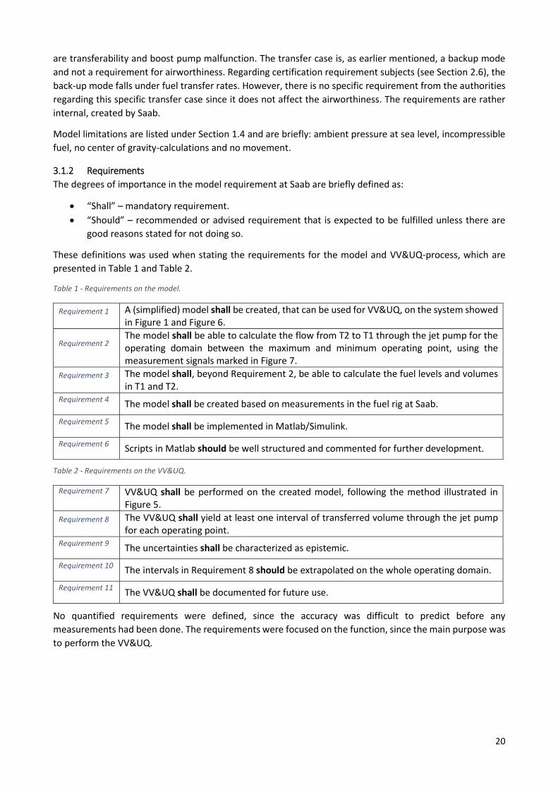
20
are transferability and boost pump malfunction. The transfer case is, as earlier mentioned, a backup mode
and not a requirement for airworthiness. Regarding certification requirement subjects (see Section 2.6), the
back-up mode falls under fuel transfer rates. However, there is no specific requirement from the authorities
regarding this specific transfer case since it does not affect the airworthiness. The requirements are rather
internal, created by Saab.
Model limitations are listed under Section 1.4 and are briefly: ambient pressure at sea level, incompressible
fuel, no center of gravity-calculations and no movement.
3.1.2 Requirements
The degrees of importance in the model requirement at Saab are briefly defined as:
“Shall” – mandatory requirement.
“Should” – recommended or advised requirement that is expected to be fulfilled unless there are
good reasons stated for not doing so.
These definitions was used when stating the requirements for the model and VV&UQ-process, which are
presented in Table 1 and Table 2.
Table 1 - Requirements on the model.
Requirement 1 A (simplified) model shall be created, that can be used for VV&UQ, on the system showed in Figure 1 and Figure 6.
Requirement 2 The model shall be able to calculate the flow from T2 to T1 through the jet pump for the operating domain between the maximum and minimum operating point, using the measurement signals marked in Figure 7.
Requirement 3 The model shall, beyond Requirement 2, be able to calculate the fuel levels and volumes in T1 and T2.
Requirement 4 The model shall be created based on measurements in the fuel rig at Saab.
Requirement 5 The model shall be implemented in Matlab/Simulink.
Requirement 6 Scripts in Matlab should be well structured and commented for further development.
Table 2 - Requirements on the VV&UQ.
Requirement 7 VV&UQ shall be performed on the created model, following the method illustrated in Figure 5.
Requirement 8 The VV&UQ shall yield at least one interval of transferred volume through the jet pump for each operating point.
Requirement 9 The uncertainties shall be characterized as epistemic.
Requirement 10 The intervals in Requirement 8 should be extrapolated on the whole operating domain.
Requirement 11 The VV&UQ shall be documented for future use.
No quantified requirements were defined, since the accuracy was difficult to predict before any
measurements had been done. The requirements were focused on the function, since the main purpose was
to perform the VV&UQ.

21
3.2 DEVELOP MODEL- AND VV&UQ-PLAN In this section, the produced plan for model development and VV&UQ is presented.
Figure 7 – Simplified block diagram with measurement signals marked in red.
In Figure 7 a simplified block diagram of the system is shown, which represents how the system should be
modelled. The two different pumps will be modelled with graphs for different operating points, where losses
in pipes, strainers and other components will be included. These components can be seen as constant
pressure losses according to experts at Saab. The modelling principle can be classed as black-box
identification, since the models will be created with polynomial curve fits rather than physical equations. This
will cause uncertainties, but lumping them together in a single model reduces the work effort greatly. Since
the components will affect the pressure in the same way when measuring for the pump graphs and when
testing the real transfer mode, the impact on the result is less significant. The operating points specified in
fuel mass flow to the engine are:
�̇� =
{
�̇�1
�̇�2
�̇�3
�̇�4
�̇�5
There are also five different initial fuel levels in T1, defined as:
ℎ1{𝑡=0} =
{
ℎ1,#1
{𝑡=0}
ℎ1,#2{𝑡=0}
ℎ1,#3{𝑡=0}
ℎ1,#4{𝑡=0}
ℎ1,#5{𝑡=0}
This results in 25 operating modes, and therefore 25 VV&UQ-evaluations are required for the simulation
model.
To obtain a pump graph for the transfer pump, all tanks except T1 will be empty and the engine will run at
different �̇�. The pump runs at full speed, which results in a surface with the pressure 𝑝 in relation to ℎ1 and
�̇�. The jet pump graph will be calculated for different 𝑝 with full power in the transfer pump, where the
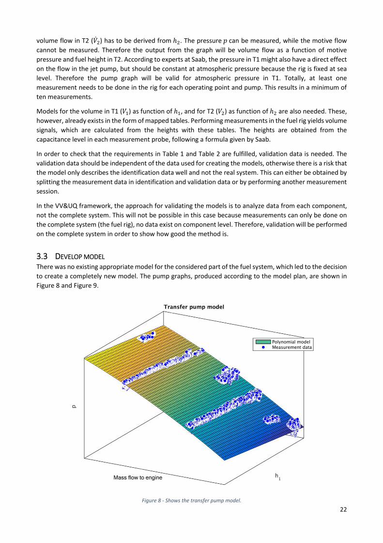
22
volume flow in T2 (�̇�2) has to be derived from ℎ2. The pressure 𝑝 can be measured, while the motive flow
cannot be measured. Therefore the output from the graph will be volume flow as a function of motive
pressure and fuel height in T2. According to experts at Saab, the pressure in T1 might also have a direct effect
on the flow in the jet pump, but should be constant at atmospheric pressure because the rig is fixed at sea
level. Therefore the pump graph will be valid for atmospheric pressure in T1. Totally, at least one
measurement needs to be done in the rig for each operating point and pump. This results in a minimum of
ten measurements.
Models for the volume in T1 (𝑉1) as function of ℎ1, and for T2 (𝑉2) as function of ℎ2 are also needed. These,
however, already exists in the form of mapped tables. Performing measurements in the fuel rig yields volume
signals, which are calculated from the heights with these tables. The heights are obtained from the
capacitance level in each measurement probe, following a formula given by Saab.
In order to check that the requirements in Table 1 and Table 2 are fulfilled, validation data is needed. The
validation data should be independent of the data used for creating the models, otherwise there is a risk that
the model only describes the identification data well and not the real system. This can either be obtained by
splitting the measurement data in identification and validation data or by performing another measurement
session.
In the VV&UQ framework, the approach for validating the models is to analyze data from each component,
not the complete system. This will not be possible in this case because measurements can only be done on
the complete system (the fuel rig), no data exist on component level. Therefore, validation will be performed
on the complete system in order to show how good the method is.
3.3 DEVELOP MODEL There was no existing appropriate model for the considered part of the fuel system, which led to the decision
to create a completely new model. The pump graphs, produced according to the model plan, are shown in
Figure 8 and Figure 9.
Figure 8 - Shows the transfer pump model.

23
Figure 9 - Shows the jet pump graph.
The following equations describes the causality and dependency in the system, where a superscript {𝑡}
corresponds to the time step 𝑡 and Δ𝑡 is the step length:
𝑝{𝑡} = 𝑝 (�̇�{𝑡}, ℎ1{𝑡}) (10)
ℎ1{𝑡} = ℎ1
{𝑡−1} + ℎ̇1{𝑡−1}Δ𝑡 𝑓𝑜𝑟 𝑡 > 0 (11)
ℎ̇1{𝑡} = ℎ̇1 (�̇�1
{𝑡}, 𝑉1{𝑡} (ℎ1
{𝑡})) (12)
𝑉1{𝑡} (ℎ1
{𝑡}) = 𝑓1 (ℎ1
{𝑡}) (13)
�̇�1{𝑡} = −�̇�2
{𝑡} −�̇�{𝑡}
𝜌𝑓𝑢𝑒𝑙 (14)
�̇�2{𝑡} = �̇�2 (𝑝 (�̇�
{𝑡}, ℎ1{𝑡}) , ℎ1
{𝑡}, ℎ2{𝑡}) (15)
ℎ2{𝑡}= ℎ2
{𝑡−1}+ ℎ̇2
{𝑡−1}Δ𝑡 𝑓𝑜𝑟 𝑡 > 0 (16)
ℎ̇2{𝑡}= ℎ̇2 ( �̇�2
{𝑡}, 𝑉2{𝑡} (ℎ2
{𝑡})) (17)
𝑉2{𝑡} (ℎ2
{𝑡}) = 𝑓2 (ℎ2
{𝑡}) (18)

24
(10) and (15) describes the two different pump graphs. (11) and (16) were created by using a first order Taylor
expansion, and by assuming the derivative as constant on a sample interval. 𝑓1 and 𝑓2 in (13) and (18) were
represented as look-up tables where linear interpolation was used to calculate values between the
measurement points. Assuming that the derivatives are zero when 𝑡 < 0 and with �̇�, ℎ1{0}, ℎ2{0}
as inputs,
the equation system in (10)-(18) has full causality and can be solved for 𝑡 ≥ 0. The earlier mentioned purpose
of the transfer case (Section 3.1.1) could mathematically be controlled by checking if the following expression
was true:
𝑉2{0}− 𝑉2
{𝑡=𝑡(ℎ1=ℎ1,𝑚𝑖𝑛,𝑙𝑖𝑚)} ≥ 𝑉2,𝑡𝑟𝑎𝑛𝑠𝑓𝑒𝑟 (19)
Where ℎ1 was calculated from (11) and 𝑉2 was calculated from (18).
Combining (12)-(14) gave the following expression for calculating ℎ̇1{𝑡}:
ℎ̇1{𝑡}=𝑑 (𝑓1
−1 (𝑉1{𝑡}))
𝑑𝑡= 𝑓1
−1̇ (𝑉1{𝑡}) ∗ �̇�1
{𝑡}= 𝑓1
−1̇ (𝑓1 (ℎ1{𝑡})) ∗ (−�̇�2
{𝑡}−�̇�{𝑡}
𝜌𝑓𝑢𝑒𝑙) (20)
In the same way, (17) and (18) could be used to calculate ℎ̇2{𝑡}
:
ℎ̇2{𝑡} = 𝑓2
−1̇ (𝑓2 (ℎ2{𝑡})) ∗ �̇�2
{𝑡} (21)
Since linear interpolation was used when evaluating 𝑓1 and 𝑓2, the inverse functions 𝑓1−1 and 𝑓2
−1 would also
be linear between the table break points. The derivatives 𝑓1−1̇ and 𝑓2
−1̇ were therefore constant between
each break point, where each constant could be calculated as the slope between the corresponding break
points.
3.4 VV&UQ In this section, the execution of the VV&UQ methodology is documented. The uncertainties identified in the
simulation model will be presented in tabular form as shown in Table 3.
Table 3 - Template for uncertainty presentation.
Label Category Component Uncertainty Description
3.4.1 Numerical uncertainty
In this section, it is described how the numerical uncertainties due to discretization-, incomplete iteration-,
solver-errors and coding mistakes were handled.
One uncertainty aroused when approximating the derivative as constant over a sample interval in the
discretization of the tank level calculations in (11) and (16). The Taylor expansion with remainder [26], is
defined as follows:
ℎ𝑇𝑎𝑦𝑙𝑜𝑟{𝑡+Δ𝑡} = ℎ{𝑡} + Δ𝑡 ∗ ℎ̇{𝑡} +
Δ𝑡2
2ℎ̈{𝜉𝑡} (22)
where 𝜉𝑡 ∈ [𝑡, 𝑡 + Δ𝑡] gives the maximum value of ℎ̈{𝜉𝑡} in the interval [26]. The third term can be seen as
the error in a first order Taylor expansion. Subtracting this to either (11) or (16) gives:

25
ℎ{𝑡+Δ𝑡} − ℎ𝑇𝑎𝑦𝑙𝑜𝑟
{𝑡+Δ𝑡}= −
Δ𝑡2
2ℎ̈{𝜉𝑡} (23)
Since the model was supposed to handle stationary cases, the second derivative should be close to zero.
However, this requires that the second derivative of ℎ exists. This might not be the case, therefore different
step lengths was tested to see how the SRQ depended on step length. The step lengths tested was 1 s, 0.2 s,
0.04 s, 0.008 s and 0.0016 s. The relative difference between the outputs for each change in step length were:
0.1 % (from 1 s to 0.2 s), 0.05 % (from 0.2 s to 0.04 s), 0.008 % (from 0.04 s to 0.008 s) and 0.002 % (from
0.008 s to 0.0016 s). A step length of 0.04 seconds was chosen because the relative difference to the next
step length was considered to be small enough, a good compromise between simulation time and accuracy.
A comparison between the outputs at the different step lengths can be seen in Figure 10.
Figure 10 - Comparison of step length.
A differential equation is explicit if the wanted value 𝑥𝑛+1 only exists on one side of the equation, the value
can then be directly calculated from previous time steps. Otherwise, the differential equation is considered
implicit and an equation system needs to be solved to obtain the wanted value [5]. According to [15], if the
mathematical problem (the model) is an initial-boundary problem and an explicit algorithm is used, no
iteration error will occur. It does not matter if the problem is linear or nonlinear when using an explicit
algorithm. When using an implicit algorithm, the problem must be linear in order to use the direct approach.
In these cases, no uncertainty from incomplete iteration will exist. The simulation model in this thesis is of
this type, and therefore it was assumed that no incomplete iteration uncertainty was present. The
approximation in calculating the height in the tanks for the next time step is of discrete character and
therefore a discrete solver was used.
When a model is completely discrete, i.e. has no continuous states, a discrete solver is automatically chosen
in Simulink. A variable and a fixed step discrete solver exist. The accuracy of the discrete fixed-step solver
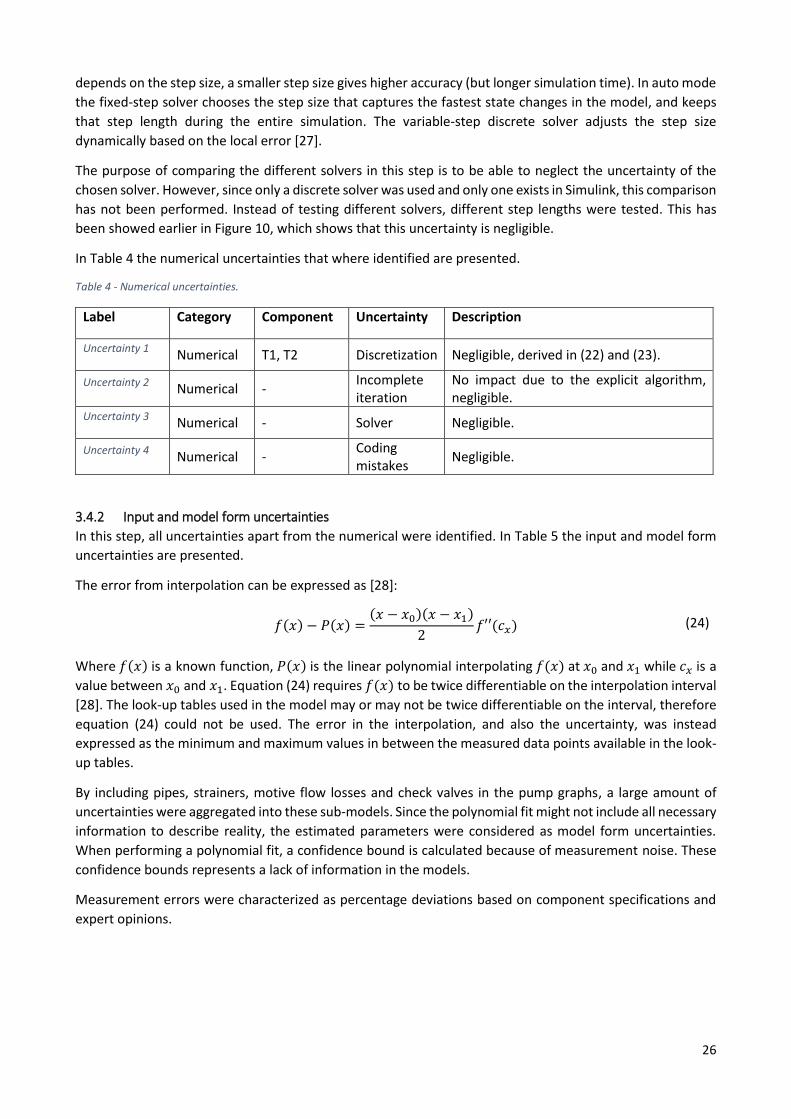
26
depends on the step size, a smaller step size gives higher accuracy (but longer simulation time). In auto mode
the fixed-step solver chooses the step size that captures the fastest state changes in the model, and keeps
that step length during the entire simulation. The variable-step discrete solver adjusts the step size
dynamically based on the local error [27].
The purpose of comparing the different solvers in this step is to be able to neglect the uncertainty of the
chosen solver. However, since only a discrete solver was used and only one exists in Simulink, this comparison
has not been performed. Instead of testing different solvers, different step lengths were tested. This has
been showed earlier in Figure 10, which shows that this uncertainty is negligible.
In Table 4 the numerical uncertainties that where identified are presented.
Table 4 - Numerical uncertainties.
Label Category Component Uncertainty Description
Uncertainty 1 Numerical T1, T2 Discretization Negligible, derived in (22) and (23).
Uncertainty 2 Numerical -
Incomplete iteration
No impact due to the explicit algorithm, negligible.
Uncertainty 3 Numerical - Solver Negligible.
Uncertainty 4 Numerical -
Coding mistakes
Negligible.
3.4.2 Input and model form uncertainties
In this step, all uncertainties apart from the numerical were identified. In Table 5 the input and model form
uncertainties are presented.
The error from interpolation can be expressed as [28]:
𝑓(𝑥) − 𝑃(𝑥) =
(𝑥 − 𝑥0)(𝑥 − 𝑥1)
2𝑓′′(𝑐𝑥) (24)
Where 𝑓(𝑥) is a known function, 𝑃(𝑥) is the linear polynomial interpolating 𝑓(𝑥) at 𝑥0 and 𝑥1 while 𝑐𝑥 is a
value between 𝑥0 and 𝑥1. Equation (24) requires 𝑓(𝑥) to be twice differentiable on the interpolation interval
[28]. The look-up tables used in the model may or may not be twice differentiable on the interval, therefore
equation (24) could not be used. The error in the interpolation, and also the uncertainty, was instead
expressed as the minimum and maximum values in between the measured data points available in the look-
up tables.
By including pipes, strainers, motive flow losses and check valves in the pump graphs, a large amount of
uncertainties were aggregated into these sub-models. Since the polynomial fit might not include all necessary
information to describe reality, the estimated parameters were considered as model form uncertainties.
When performing a polynomial fit, a confidence bound is calculated because of measurement noise. These
confidence bounds represents a lack of information in the models.
Measurement errors were characterized as percentage deviations based on component specifications and
expert opinions.
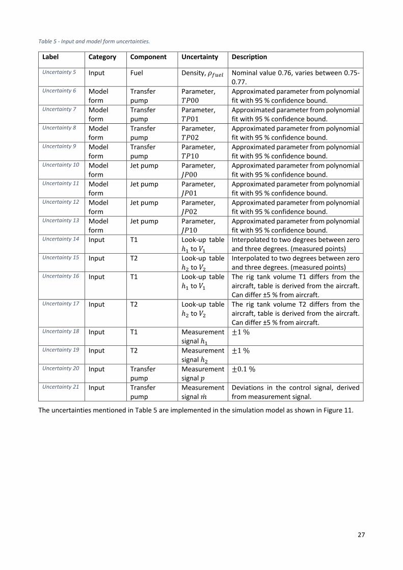
27
Table 5 - Input and model form uncertainties.
Label Category Component Uncertainty Description
Uncertainty 5 Input Fuel Density, 𝜌𝑓𝑢𝑒𝑙 Nominal value 0.76, varies between 0.75-0.77.
Uncertainty 6 Model form
Transfer pump
Parameter, 𝑇𝑃00
Approximated parameter from polynomial fit with 95 % confidence bound.
Uncertainty 7 Model form
Transfer pump
Parameter, 𝑇𝑃01
Approximated parameter from polynomial fit with 95 % confidence bound.
Uncertainty 8 Model form
Transfer pump
Parameter, 𝑇𝑃02
Approximated parameter from polynomial fit with 95 % confidence bound.
Uncertainty 9 Model form
Transfer pump
Parameter, 𝑇𝑃10
Approximated parameter from polynomial fit with 95 % confidence bound.
Uncertainty 10 Model form
Jet pump Parameter, 𝐽𝑃00
Approximated parameter from polynomial fit with 95 % confidence bound.
Uncertainty 11 Model form
Jet pump Parameter, 𝐽𝑃01
Approximated parameter from polynomial fit with 95 % confidence bound.
Uncertainty 12 Model form
Jet pump Parameter, 𝐽𝑃02
Approximated parameter from polynomial fit with 95 % confidence bound.
Uncertainty 13 Model form
Jet pump Parameter, 𝐽𝑃10
Approximated parameter from polynomial fit with 95 % confidence bound.
Uncertainty 14 Input T1 Look-up table ℎ1 to 𝑉1
Interpolated to two degrees between zero and three degrees. (measured points)
Uncertainty 15 Input T2 Look-up table ℎ2 to 𝑉2
Interpolated to two degrees between zero and three degrees. (measured points)
Uncertainty 16 Input T1 Look-up table ℎ1 to 𝑉1
The rig tank volume T1 differs from the aircraft, table is derived from the aircraft. Can differ ±5 % from aircraft.
Uncertainty 17 Input T2 Look-up table ℎ2 to 𝑉2
The rig tank volume T2 differs from the aircraft, table is derived from the aircraft. Can differ ±5 % from aircraft.
Uncertainty 18 Input T1 Measurement signal ℎ1
±1 %
Uncertainty 19 Input T2 Measurement signal ℎ2
±1 %
Uncertainty 20 Input Transfer pump
Measurement signal 𝑝
±0.1 %
Uncertainty 21 Input Transfer pump
Measurement signal �̇�
Deviations in the control signal, derived from measurement signal.
The uncertainties mentioned in Table 5 are implemented in the simulation model as shown in Figure 11.
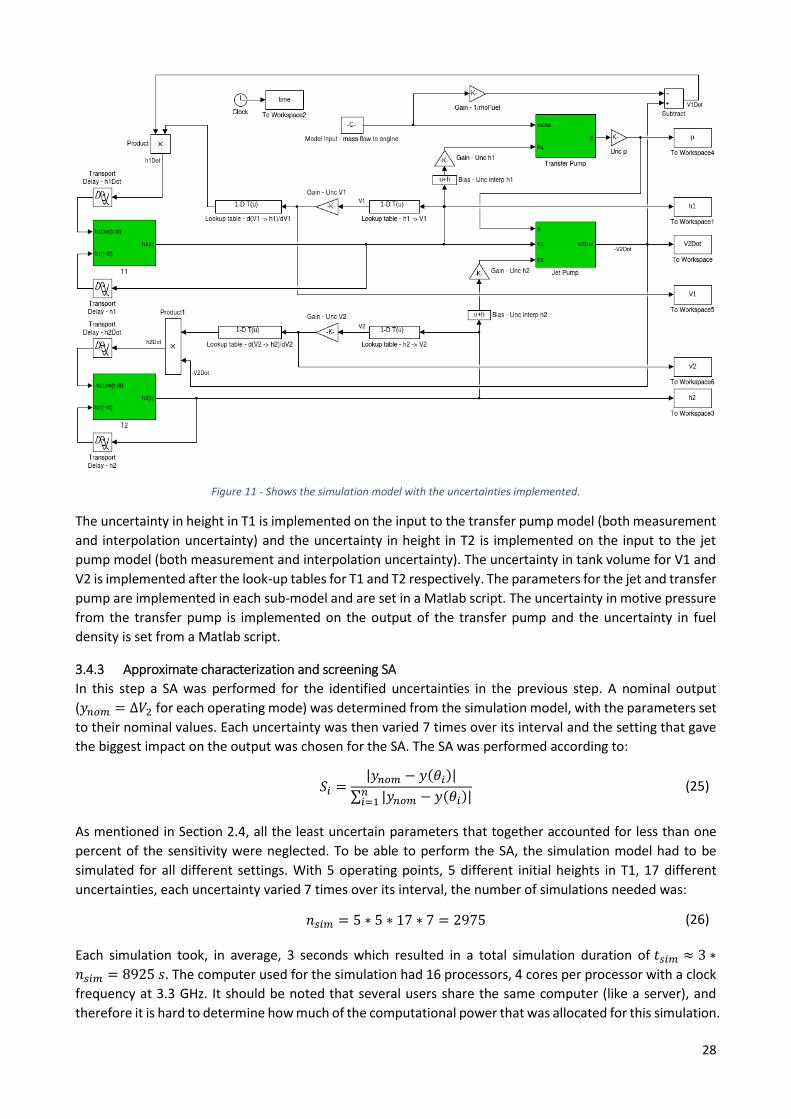
28
Figure 11 - Shows the simulation model with the uncertainties implemented.
The uncertainty in height in T1 is implemented on the input to the transfer pump model (both measurement
and interpolation uncertainty) and the uncertainty in height in T2 is implemented on the input to the jet
pump model (both measurement and interpolation uncertainty). The uncertainty in tank volume for V1 and
V2 is implemented after the look-up tables for T1 and T2 respectively. The parameters for the jet and transfer
pump are implemented in each sub-model and are set in a Matlab script. The uncertainty in motive pressure
from the transfer pump is implemented on the output of the transfer pump and the uncertainty in fuel
density is set from a Matlab script.
3.4.3 Approximate characterization and screening SA
In this step a SA was performed for the identified uncertainties in the previous step. A nominal output
(𝑦𝑛𝑜𝑚 = Δ𝑉2 for each operating mode) was determined from the simulation model, with the parameters set
to their nominal values. Each uncertainty was then varied 7 times over its interval and the setting that gave
the biggest impact on the output was chosen for the SA. The SA was performed according to:
𝑆𝑖 =
|𝑦𝑛𝑜𝑚 − 𝑦(𝜃𝑖)|
∑ |𝑦𝑛𝑜𝑚 − 𝑦(𝜃𝑖)|𝑛𝑖=1
(25)
As mentioned in Section 2.4, all the least uncertain parameters that together accounted for less than one
percent of the sensitivity were neglected. To be able to perform the SA, the simulation model had to be
simulated for all different settings. With 5 operating points, 5 different initial heights in T1, 17 different
uncertainties, each uncertainty varied 7 times over its interval, the number of simulations needed was:
𝑛𝑠𝑖𝑚 = 5 ∗ 5 ∗ 17 ∗ 7 = 2975 (26)
Each simulation took, in average, 3 seconds which resulted in a total simulation duration of 𝑡𝑠𝑖𝑚 ≈ 3 ∗
𝑛𝑠𝑖𝑚 = 8925 𝑠. The computer used for the simulation had 16 processors, 4 cores per processor with a clock
frequency at 3.3 GHz. It should be noted that several users share the same computer (like a server), and
therefore it is hard to determine how much of the computational power that was allocated for this simulation.

29
For each of the 17 uncertainties, a nominal output and the output that had the biggest deviation from the
nominal output was stored for each operating point and initial height. Using equation (25), this resulted in
the sensitivity for all stored data points. After the reduction of uncertainties in the SA, the remaining
uncertainties for the five different operating points are shown in Table 6:
Table 6 - Remaining uncertainties after SA for all operating points.
Operating point Remaining uncertainties
1 Uncertainty 15, Uncertainty 17
2 Uncertainty 15, Uncertainty 17
3 Uncertainty 5, Uncertainty 10, Uncertainty 11, Uncertainty 12, Uncertainty 13, Uncertainty 14, Uncertainty 15, Uncertainty 16, Uncertainty 17, Uncertainty 19, Uncertainty 20, Uncertainty 21
4 Uncertainty 5, Uncertainty 7, Uncertainty 10, Uncertainty 11, Uncertainty 12, Uncertainty 13, Uncertainty 14, Uncertainty 15, Uncertainty 16, Uncertainty 17, Uncertainty 19, Uncertainty 20, Uncertainty 21
5 Uncertainty 5, Uncertainty 7, Uncertainty 8, Uncertainty 10, Uncertainty 11, Uncertainty 12, Uncertainty 13, Uncertainty 14, Uncertainty 15, Uncertainty 16, Uncertainty 17, Uncertainty 19, Uncertainty 20, Uncertainty 21
For operating point one and two, 15 of the 17 uncertainties could be ignored. For operating point three, 5 of
the 17 uncertainties could be ignored. For operating point four, 4 of the 17 uncertainties could be ignored.
For operating point five, 3 of the 17 uncertainties could be ignored.
The SRQ of interest here, Δ𝑉2, was highly dependent on the operating point and the initial height in T1. The
simulation stopped when the fuel level in T1 reached ℎ1,𝑚𝑖𝑛,𝑙𝑖𝑚 and this point was reached after a specific
simulation time. Depending on the operating point and initial height, the simulation time varied greatly (at
most ~600 s). With higher fuel flow to the engine and a low initial height, the simulation time was shorter,
while for the opposite case, the simulation time was longer. This caused the uncertainties to have a widely
different impact on the SRQ depending on operating point. As seen in Table 6, many uncertainties could be
ignored in operating point 1 and 2, while for the remaining operating points only a few uncertainties could
be ignored. At the two first operating points a larger amount of fuel was transferred. Because of the lower
fuel flow to the engine, T1 is emptied slower and in addition a higher induced flow through the jet pump is
obtained. This means that all the fuel in T2 is transferred to T1 before ℎ1,𝑚𝑖𝑛,𝑙𝑖𝑚 was reached. The only two
uncertainties that mattered in this case were those with direct impact on the initial volume in T2, since they
affected how much fuel that could be transferred. Of the other operating points, number three was the one
that simulated the longest. In this case, the uncertainties were iterated more than in the other points which
means that they had a larger effect.
To get rid of the effect of different simulation times, a SA was performed where the simulation model was
run for a specific time, 𝑡𝑠𝑖𝑚, at all operating points. This means that the uncertainties were iterated the same
amount of times for all operating points, and the effect of the uncertainties at the different operating points
could therefore be compared in a better way. In Table 7, the remaining uncertainties for this case are
presented.

30
Table 7 - Remaining uncertainties after SA, constant simulation time for all operating points.
Operating point Remaining uncertainties
1 Uncertainty 10, Uncertainty 11, Uncertainty 12, Uncertainty 13, Uncertainty 16, Uncertainty 17, Uncertainty 19
2 Uncertainty 10, Uncertainty 11, Uncertainty 12, Uncertainty 13, Uncertainty 17, Uncertainty 19, Uncertainty 21
3 Uncertainty 10, Uncertainty 11, Uncertainty 12, Uncertainty 13, Uncertainty 17, Uncertainty 19, Uncertainty 20, Uncertainty 21
4 Uncertainty 7, Uncertainty 8, Uncertainty 10, Uncertainty 11, Uncertainty 12, Uncertainty 13, Uncertainty 16, Uncertainty 17, Uncertainty 19, Uncertainty 20, Uncertainty 21
5 Uncertainty 7, Uncertainty 8, Uncertainty 10, Uncertainty 11, Uncertainty 12, Uncertainty 13, Uncertainty 16, Uncertainty 17,Uncertainty 18, Uncertainty 19, Uncertainty 20, Uncertainty 21
As seen in Table 7, the amount of uncertainties are more similar for the different operating points in
comparison to the first case. In the first three operating points, 9 of the 17 uncertainties could be neglected.
For operating point four and five, 6 and 5 uncertainties could be neglected respectively.
3.4.4 Detailed characterization
The detailed characterization is more relevant when handling aleatory uncertainties. In the case of only
epistemic uncertainties, the determined interval in which the uncertainty can vary could be chosen more
precisely. However, due to limited access to measurement data these intervals could not be improved further.
The uncertainty due to the confidence bounds of the jet pump parameters seemed to have a big impact on
the SRQ, this is one area where the bounds could have been improved (i.e. reduced) with more measurement
data.
3.4.5 Minimum/maximum parameter settings
In this step the transfer pump and jet pump sub-models were analyzed as stand-alone models. The
uncertainty in the look-up tables for T1 and T2 were given as percentage values, meaning that the minimum
limit would give the minimum output, and vice versa for the maximum limit. These models were therefore
not analyzed further in this step. Given an input to each model, the output was calculated according to
equation (27) (previously mentioned in Section 2.4):
𝑦 = 𝑦𝑛𝑜𝑚 + ∑ Δ𝑥𝑖𝛽𝑖𝑚𝑖=1 (27)
For the transfer pump, the input was height in T1 and the output was the pressure. For the jet pump, the
input was pressure and height in T2, and the output was the induced flow. The relationship between 𝑝 and
ℎ1 was found to be linear, meaning that ℎ1 could be set as constant for the transfer pump. In the same way,
the relationship between �̇�2 and ℎ2 was linear and therefore ℎ2 was set as constant for the jet pump. This
meant that the minimum/maximum settings would be the lowest and highest boundary values for each
uncertainty, there was therefore no need to vary ℎ1 or ℎ2 during the analysis. The relationship between flow
and pressure in the models was found to be more quadratic than linear, therefore LHS was used to conclude
which parameter settings that resulted in minimum/maximum output. 10 LHS samples was used for each
uncertainty and an estimate of 𝛽𝑖 was calculated using the least square-method according to:
�̂� = (ΔXTΔ𝑋)
−1Δ𝑋𝑇Δ𝑌
(28)
where

31
Δ𝑋 = [
𝛥𝑥1,1 … 𝛥𝑥1,𝑚⋮ ⋱ ⋮
𝛥𝑥𝑁,1 … 𝛥𝑥𝑁,𝑚
] , Δ𝑌 = [𝛥𝑦1(𝜙(1)) … 𝛥𝑦1(𝜙(𝑒𝑛𝑑))
⋮ ⋱ ⋮𝛥𝑦𝑁(𝜙(1)) … 𝛥𝑦𝑁(𝜙(𝑒𝑛𝑑))
]
The 𝜙 vector was the input to the corresponding sub-models. In this case, only the jet pump required a varied
input (motive pressure). For the transfer pump, Δ𝑌 was a column vector instead of a matrix as for the jet
pump. The estimated 𝛽𝑖 was on the form:
�̂� = [�̂�1(𝜙(1)) … �̂�1(𝜙(𝑒𝑛𝑑))
⋮ ⋱ ⋮�̂�𝑚(𝜙(1)) … �̂�𝑚(𝜙(𝑒𝑛𝑑))
]
Equation (28) was evaluated five times, one for each operating point �̇�. Depending on the operating point
and sub-model, Δ𝑋 and Δ𝑌 had different dimensions because of the amount of neglected uncertainties in
that operating point.
�̂�𝑖(𝜙) corresponds to the slope in which the output varies with respect to the uncertainty 𝑖, for the specific
input value 𝜙 . The sign of �̂�𝑖(𝜙) tells whether the output increases/decreases with an increase in the
uncertain parameter. In this way the minimum/maximum parameter setting could be determined as the
upper/lower or lower/upper bound for the uncertain parameter, depending on the sign of �̂�𝑖(𝜙).
3.4.6 Uncertainty propagation at top level
In this step, the information gained from the previous steps was used to propagate the minimum/maximum
outputs from the different sub-models in the total simulation model. With the minimum/maximum
parameter settings for each sub-model determined, it was also necessary to determine how the settings for
each sub-model should be combined with the other sub-models. For example, the minimum settings for the
jet pump and maximum settings for the transfer pump may result in the maximum value of the SRQ. This
combination of parameter settings for the sub-models therefore had to be determined before proceeding
with the uncertainty propagation at top level. This could be done by varying the output of a sub-model and
see how it affected the SRQ in the total simulation model. The behavior of the uncertainty in volume for T1
and T2 proved to be non-linear with respect to the SRQ, which is shown in Figure 12 and Figure 13, the
minimum/maximum settings varied both for operating point and initial height. These parameter settings
were found by varying, one at a time, V1 and V2 and finding where the minimum/maximum output in the
SRQ was obtained.

32
Figure 12 - Shows how the SRQ varies when the uncertainty in V1 is varied.
Figure 13 - Shows how the SRQ varies when the uncertainty in V2 is varied.

33
The other uncertainties were considered to have a linear effect on the SRQ (see Figure 14 for an example and
Appendix A for the remaining uncertainties). When these combinations were determined, the uncertainty
propagation at top level was performed. This resulted in two simulations with a minimum and a maximum
response in the SRQ for each operating mode.
Figure 14 - Shows how the SRQ varies when the uncertainty in h2 is varied.
To check the validity of the minimum and maximum response, LHS was used to vary all uncertain parameters
in the model in a random way. This was done in order to see that all responses produced by the LHS-
simulations were within the minimum and maximum response. One LHS simulation was performed for the
first case (total transferred volume at each operating point) and one LHS simulation for the second case
(transferred volume at each operating point during 𝑡𝑠𝑖𝑚 ). The number of LHS samples chosen for both
simulations were 5000, since the amount of samples that should be chosen were at least 𝑚3 = 4913 (see
Section 2.5). The simulations were performed for the five different operating points and for five different
initial heights in T1. This results in 125000 simulations for each case. For the first case, one simulation took
in average 1.2 seconds. The total simulation time was, for the first case, approximately 125000 ∗ 1.2𝑠 =
150000𝑠 ≈ 42ℎ. For the second case, one simulation took in average 0.5 seconds which resulted in a total
simulation time of 125000 ∗ 0.5𝑠 = 62500𝑠 ≈ 17ℎ.
3.4.7 Validation and inter-/extrapolation of uncertainties
In order to inter-/extrapolate the uncertainties at different fuel flows to the engine (�̇�) or different initial
tank levels in T1 (ℎ1{𝑡=0}
) validation data is required along with an analysis of the input uncertainties. In
Requirement 10 it is stated that the epistemic intervals should be extrapolated over the whole operation
domain, which means for all fuel mass flows to the engine between �̇�1 − �̇�5. Validation measurements were
performed for operating point 3-5, since the first two operating points causes a larger in-flow to T1 than out-
flow, and therefore will empty all fuel in T2. Only two different ℎ1{0}
where chosen, ℎ1,#2{𝑡=0} and ℎ1,#4
{𝑡=0}, due to
lack of time in the fuel rig.

34
The results from the validation measurements is presented under Section 4.3, and it can be said that they all
were inside of the epistemic intervals derived for the corresponding inputs. This meant that the area
validation metrics were all equal to zero, which gave the following regression based on (4):
�̂� = 0 (29)
Inserting (29) in (6) gave:
𝑠 = √∑(𝑦𝑖 − �̂�𝑖)
2
𝑁 − 2
𝑁
𝑖=1
= 0 (30)
Thereafter (29),(30) were inserted in (5) which ultimately led to the following expression for the prediction
interval:
�̂� ± 𝑡𝛼2,𝑁−𝑏
𝑠√1 +1
𝑁+
𝑁(𝑥 − �̅�)2
𝑁∑ 𝑥𝑖2 − (∑ 𝑥𝑖𝑁 )2)𝑁
= 0 (31)
Due to this trivial outcome of the prediction interval and the lack of time in the fuel rig, the interpolation was
not proceeded. The procedure would require new measurements in the rig to determine input uncertainties,
since only the model form uncertainties are interpolated. After this the same VV&UQ-procedure would have
been performed as for the five evaluated operating points, which was not considered to bring anything new
to the evaluation of the VV&UQ-methodology.

35
4 RESULTS
In this section, the results from the thesis are presented.
4.1 TOTAL UNCERTAINTY The result of the uncertainty propagation in the VV&UQ for the first case is shown in Figure 15. For the first
two operating points all fuel from T2 is transferred to T1, for all initial heights. For the third operating point,
it can be guaranteed that the transfer limit can be reached for the two last initial heights. For operating point
four, this cannot be guaranteed because the minimum amount of fuel transferred never goes above the
transfer limit. In the fifth operating point, the determined transfer limit can in fact never be achieved because
all points are beneath the limit. The same scale is used for all x- and y-axes in the figure.
Figure 15 - Shows the minimum and maximum transferred volumes after the VV&UQ-evaluation of the first case.
In Figure 16, the result of the uncertainty propagation for the second case is shown. It shows that for a higher
fuel flow to the engine, less fuel is transferred from T2 to T1. In operating point one, less fuel is transferred
for the last initial height because T1 gets full. The same scale is used for all x- and y-axes in the figure.
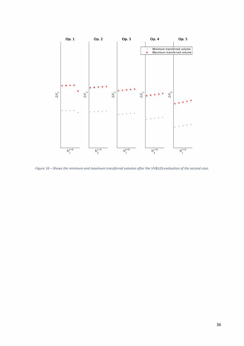
36
Figure 16 – Shows the minimum and maximum transferred volumes after the VV&UQ-evaluation of the second case.

37
4.2 VALIDITY CHECK OF MIN/MAX PARAMETER SETTINGS As mentioned in Section 3.4.6, LHS was performed on the simulation models for both the first and second
case. Figure 17 shows the validity check for the first case and Figure 18 for the second case.
Figure 17 - Shows the minimum and maximum output in the SRQ together with the minimum transfer limit for the different operating modes, for first case with total transferred volume at each operating point.
After doing the validity check, it could be seen that all LHS-simulations produced outputs in the SRQ that was
inside the min/max simulations for the second case. For the first case, there was one LHS-simulation that was
outside of the min/max simulations. This point was 0.78 % smaller than the minimum transferred volume
(for operating point five, highest initial height).

38
Figure 18 - Shows the minimum and maximum output in the SRQ together with the minimum transfer limit for the different operating modes, for second case with transferred volume at each operating point during 𝑡𝑠𝑖𝑚.

39
4.3 VALIDATION Validation of the simulation model was performed in the fuel rig for the first transfer case for operating point
three, four and five. Two different initial heights were tested for each of the three operating points. The
result of the validation is shown in Figure 19.
Figure 19 - Shows the validation data, nominal simulation output and min/max output.
As can be seen, the validation data is placed between the min/max outputs for all validation measurements.

40
5 DISCUSSION
In this section, the method and results in this thesis are discussed.
5.1 RESULTS The resulting min/max simulations shows what the worst/best scenarios looks like, but not how often one
can expect the transferred volume to be the minimum or maximum amount. This is because we have only
considered epistemic uncertainties, no statistical information is incorporated in the uncertainties. This is a
downside of the methodology, we might be able to tell how the worst/best scenarios looks like, but not how
probable they are of occurring. In the case of fighter aircrafts, there is an error tolerance of 1 in a million.
This translates into a probability for something critical happening of 0.0001 percent, which then means that
characterizing the uncertainties as epistemic should be enough. An epistemic characterization requires less
knowledge of the system than an aleatory characterization, it is also less time consuming to evaluate and this
were the reasons for the epistemic characterization in the framework that has been used in the thesis. It may
also be an advantage to use an epistemic characterization if you only want to know if an error can occur, not
how often it can occur. If that is the case, you do not need the additional information that an aleatory
characterization provides and the workload will be reduced.
As seen in Figure 15, it is clear from the result that we will always be capable of transferring enough fuel for
operating points one and two. In operating point three we can guarantee that enough fuel will be transferred
for a certain fuel flow to the engine, given that the fuel transfer starts at a given fuel level in T1. This can be
guaranteed because the minimum amount of fuel crosses the transfer limit at a given point. The minimum
amount of transferred fuel represents the case where all components are faulty in the worst combination
with respect to the SRQ, in our case the transferred volume of fuel. For operating point four, it cannot be
guaranteed that enough fuel will be transferred but it is possible, as can be seen on the maximum simulation
result. For operating point five, we can say that the fuel transfer will never be adequate.
When comparing the total amount of transferred fuel (first case) with the amount of fuel transferred during
a specific time (second case), we see that the uncertainties have a more similar impact on the different
operating points in the second case. This is probably because the uncertainties are iterated a different
amount of times in the first case, depending on how long it takes to empty T1. The first case is the operating
condition that we are interested in, because it represents a real event in the aircraft. The second case was
performed in order to see the effects of the uncertainties in the jet pump, and this case is more general than
the first case.
In the first case, there was one point in the LHS-simulation that came outside of the min/max outputs. This
may be because some uncertainties in the min/max simulations were neglected from the SA, while all
uncertain parameters were varied in the LHS-simulation. When neglecting uncertainties in a model, a
compromise is made. In our case, 1 of 125000 points were outside the min/max output and still inside the
1 % sensitivity limit that was set in the SA. The benefit from the compromise was that the simulation time
decreased a lot when the uncertainties were neglected, the analysis became more manageable. In our
opinion, it would be reasonable to increase the max output with 1 % and decrease the minimum output with
1 % to take the neglected uncertainties into account.
The resulting intervals in the SRQ are relatively large, i.e. the difference between the min/max outputs are
large compared to the nominal output. This means that there is a lot of uncertainty in the model and this can
partly be explained by the simplifications made. We have created few models which contains many
components. When doing this, the level of detail in the model is reduced and the uncertainty increases. This
simplification was done in order to reduce the workload and make the VV&UQ feasible, as was described in
the framework. If more detailed models where used, it could result in an increased amount of uncertainties
which would make the VV&UQ impractical to perform. This can motivate the use of polynomial models

41
(identification). It all depends on how accurate the result has to be, it may be found that our result is too
uncertain or inaccurate. Then, the models must be revised or the uncertainties must be characterized in a
more accurate way. The measurement error might also be a part of the explanation to the size of the
uncertainty intervals. We could not measure the induced flow of the jet pump directly, we had to measure
the transferred amount of fuel from T2 to T1. This caused large uncertainties in the jet pumps polynomial
parameters, which were also the biggest uncertainties of all. If the induced flow could be measured directly,
this could greatly reduce the uncertainty.
Validation of the result was done for operating points three, four and five as can be seen in Figure 19. Here
it can be seen that the validation data fits inside the min/max outputs from the simulation model. The
validation data also follows the nominal output from the simulation model relatively well. For operating point
three, the validation data differs more from the nominal output than for operating point four and five. This
might be because it was hard to get the right amount of fuel in T2 (i.e. full) when the transfer started and the
fuel flow to the engine had stabilized. Because of limited access to the fuel rig, more measurements could
not be performed and the result could not be improved. Validation data was not collected for operating point
one and two because of the low fuel flow to the engine, the fuel flow into T1 was always greater than the
fuel flow out of T1. It was therefore considered irrelevant to collect validation data for these operating points.
5.2 METHOD When doing the estimation of numerical uncertainty, the goal is to be able to neglect it according to the
framework. In this thesis, the system is small but with a larger system the simulation time will increase. This
may lead to an increased step size in order to limit the simulation time and therefore the numerical
uncertainties may not be negligible. This could be a problem when analyzing a bigger system than we have
in our thesis.
In this thesis, 21 uncertainties were identified from the start. Four of these were negligible (the numerical
uncertainties) before doing further analysis. After the SA a few more could be ignored for each operating
point as described in Section 3.4.3. With this small amount of uncertainties, and with a simulation model that
is fairly un-complex, it was still time demanding to perform the LHS-simulations. This is a form of validation,
or validity check, which should be performed in order to know that the min/max simulations were correct. It
was recommended to have 𝑚3 number of LHS-samples when doing the sampling. This means that for every
added uncertainty, the number of simulations increases quickly. The methodology builds on the reduction of
the amount of uncertainties, and if there are many uncertainties it becomes time consuming despite the
simplifications done in the methodology.
The min/max approach in the framework built on the assumption that the system was fairly linear in the
operating region chosen. While this assumption was legitimate for most parts of our system, this may not be
the case for other systems. If the system is not linear the min/max approach cannot be used, the work load
will increase and it can be difficult to perform VV&UQ.
The VV&UQ-method that has been evaluated in this thesis is adapted for systems where data of the complete
system does not exist. We could only collect data from the complete system, the fuel rig, in this thesis. To
compensate for this we have tried to isolate each component when collecting identification data in order to
be as close to the methodology as possible. However, it was beneficial to be able to collect validation data of
the complete system in order to evaluate the methodology (which was the main purpose). This provides us
with information about how the components interacts in the system, which would not exist for an incomplete
system. This information would only come from the simulation model if the fuel rig did not exist. When the
model output was validated it was found to be fairly accurate. With this argumentation, we find the VV&UQ-
method to be a good way of evaluating the fuel system on a component level and to get an idea of how the
uncertainties in the different components affect the total system in the end.
42
We have not considered the ambient conditions in the test rig (temperature, pressure etc.) in the simulation
model. The effects of these conditions are assumed to be captured by the fuel density in the measurement
data. The ambient conditions cannot be determined in the model, which is a downside. This must be
controlled in the fuel rig, so that the conditions when capturing new data are as similar as possible to the
data from which the model parameters were identified. With more time, a model that takes the ambient
conditions in consideration could have been developed. This would be necessary if the fuel rig is to be
replaced by a simulation model. It might also be of interest to test other conditions than the one that has
been evaluated in this thesis, other air pressures than at sea level for example.
The jet pump is a very complex component that is difficult to model. We have created a polynomial model
that depends on the motive pressure and the fuel height in T2 and it produces an induced flow out of the
component. There might be other factors that matters more than the parameters that we have considered
when developing the model. In an article we read, the jet pump model included the ratio between induced
flow and motive flow. In our case, the induced flow could be measured indirectly in the rig by the amount of
fuel that was transferred from T2 to T1. However, the motive flow could not be measured. We did find that
the motive flow should increase with a decrease in flow to the engine, and this behavior is captured in the
model. The physical jet pump models we have seen at Saab and in other research papers are very complex
and because the focus in this thesis was to evaluate the methodology, it was considered to be too time
consuming to develop a physical model. However, if more effort were put into creating a better model, more
sensors would be needed. Outlet pressure, motive flow and induced flow are probably the most important
signals to measure apart from the ones available, based on the research we have done.
As earlier mentioned, the VV&UQ-framework depends on getting a number of uncertainties that is fairly low.
If the jet pump model was physical, the number of uncertainties would increase because the number of
parameters in the model increases. If it was possible to perform thorough measurements on the jet pump, a
number of these parameters might be considered as certain and the number of uncertainties would then
again be reduced. The result of this might be a better model, and the same could be done for other
components in the system. A benefit with using physical models is that it gets easier to understand and assess
the size and impact of an uncertainty.
The model that was produced in this thesis was constructed in such a way that several components were
lumped together in one. As earlier mentioned, this causes larger uncertainties but reduces the workload. In
our case we had to adapt to the available measurement equipment, i.e. the fuel rig, which limited our
opportunities to model each component by themselves. However, the hypothetical scenario when using
VV&UQ for certification in the future is that there is only component data available and no rig exists. This
would make it easier to evaluate each component of the system by itself. A question here is if it really is the
best way to do it? If one were to model each pipe, strainer, valve etc. it would either lead to an extremely
extensive modeling process or a huge growth in the amount of uncertainties. In the aircraft fuel system
application, which is a very complex system, it is necessary to be restrictive regarding the workload of the
chosen method. Even without a rig it is possible to lump together components, for example by attaching
valves and strainers to a pump and model them together. We believe that this is a good compromise between
workload and accuracy.

43
5.3 CERTIFICATION POTENTIAL OF SIMULATION MODELS The main subjects in the certification process are:
Defining a type design.
Provide proof that the type design complies with the requirements.
Plan and perform maintenance and inspections.
The fact that the head of the design organization is personally responsible should entail that the procedure
is thoroughly executed. It does, however, have an impact on how large part software simulations can have
on the certification. In order to trust a result from a simulation model, one has to understand how it works
or trust other people to know how it works. In a large system it is hardly possible for one person to have good
enough insight in all systems and the software models of those systems to vouch that they are good enough
to use as certification basis. Hence, it is important to have an approved methodology for designing and
evaluating simulation models. In this way, the responsibility can for example be appointed to the head of the
corresponding department to make sure that this methodology is followed correctly. It is easier for each
department to have insight and understanding of their own subsystem and software models.
When discussing whether or not software models can be used for certification or replacing a physical rig, one
must first state what the requirements are. Perhaps it is hard to cover the entire functionality that you get
from a rig, but it might not be necessary either. In the certification procedure at Saab, a large part of the
requirement compliance is demonstrated during ground tests with the real aircraft. The rig is used for a few
applications, including demonstrating compliance with lower prioritized requirements. The high cost, in time
and money, to build a rig makes it desirable to use simulation models instead. A compromise could be to use
a simulation model to cover up as many applications as possible that the rig is used for, and prolong the
duration of field tests to cover up the parts that the simulation model is unable to cover. An important subject
here is to investigate if there is actually a reduction in cost by doing this. The knowledge from this thesis is
that creating simulation models, evaluating uncertainties according to the proposed methodology and
performing all required simulations is very time demanding. It is also a possibility that the prolonging of the
field tests will give an increased cost as well. An extensive investigation of the costs in terms of time and
money could therefore be beneficial to perform before choosing one or another.
It is important to state that one of the main reasons for building the current fuel rig was that there was lack
of knowledge about the system. The fuel rig is not the real aircraft but the data collected from tests in the
fuel rig is often seen as the “truth”, when it in some cases is not. A benefit that comes with modelling is that
knowledge about the system is required if the models are to be any good. It is our belief that time and
resources should be allocated for getting to learn the system better. If good knowledge about the system is
gained, this would also result in models that people could trust more than they do today. The step to using
simulation models in the certification procedure, instead of physical test rigs, would then be reduced.
The certification of an aircraft has many different parties involved, especially since it is such a complex
product with high requirements on safety. This means that eventual mistakes in the procedure might cause
huge delays and/or that procedures has to be redone. In this matter, it is of high importance to make as few
mistakes as possible. There is always a risk that something goes wrong when working with software models,
which should be weighted when deciding whether to replace a rig or not. Of course mistakes can be made
when building and running tests in a rig, but they are easier to discover and prevent than in a simulation
model.
A challenge that is faced when considering to use software models without a physical system to test against
is that there is not possible to get validation data, at least not for the whole system. This causes a need for
alternate methods to proof the validity of the model. The investigated method for VV&UQ is adapted to an
early phase in the aircraft development, where lack of validation data is a central problem. The difference
with using simulation models for development and certification is that the certification basis should act as a

44
proof that the real product will work, while the development material will be tested further and is not a
guarantee for that the system will work completely.
Another problem with a simulation model is that it can be hard to model the behavior of a component that
is damaged, flawed or in any way deviates from the nominal component. However, this might also be hard
to see in a rig as well. Unless more than one individual of the same components in a rig is evaluated, there
will be difficulties in deciding whether or not they act nominal. Testing of different individuals, on the other
hand, can also be done in a simulation model. By performing component level validation, UQ and creating
models for different individuals of the same component, the reliability of the simulation model is increased.
In order to increase the reliability further, real hardware components can also be included to create a
“Hardware-in-the-loop”-simulation (HIL). This will also strengthen the results from simulation to be used as
certification basis.
In this thesis the tests and simulations that were performed only treated performance requirements. Even
though the question “Can the jet pump manage to transfer a volume 𝑉2,𝑡𝑟𝑎𝑛𝑠𝑓𝑒𝑟 to T1 before the fuel level
in T1 falls below a predefined level ℎ1,𝑚𝑖𝑛,𝑙𝑖𝑚?” can be answered with yes/no, the result from the VV&UQ-
analysis actually tells us how much fuel that will be transferred before ℎ1 ≤ ℎ1,𝑚𝑖𝑛,𝑙𝑖𝑚 (in terms of minimum
and maximum limits). A question that could be asked is, “is the result from the simulations and VV&UQ-
analysis enough to prove compliance with the functional requirement that this transfer mode will work in
reality?” The question does not have a definite answer, but is rather an assessment. By including the most
complex hardware components in the loop it might give results that are considered good enough to prove
compliance with functional requirements.
An important fact when dealing with (manned) aircraft systems is that ultimately a real human being is going
to fly the aircraft. The leeway for mistakes in flight-critical functions is nonexistent. This brings in a
philosophical point of view on the certification process. Can the head of design trust the simulation models
enough to convince a pilot to fly the real aircraft? Is it possible to fully prove that the aircraft works with
simulation models? On the other hand, is it possible with a rig? It is a question of where to draw the line for
when the certification basis is considered reliable enough. Based on what we have seen at Saab, there are
tendencies to put too much faith in physical rigs and therefore simulation models are rejected. An aircraft
has many complex systems that are hard to model accurately, which has caused decisions to build rigs in
order to increase knowledge and confidence in them. One part that is frequently missed (or ignored) is that
the rig is not a perfect copy of the real aircraft. There can be significant differences in components,
geometries, materials, environment and so on, which should be weighed against the flaws and insecurities
in the simulation models. With that in mind, a simulation model might not give a perfect view of reality.
However, it might still be good enough to cover up for a physical rig.
45
6 CONCLUSIONS
The fuel rig that has been analyzed is mainly used for testing functional requirements, but also to improve
knowledge about the different phenomena in the fuel system. From a certification perspective the rig is
mainly used to shorten the time in ground tests, where most of the demonstration of compliance is
performed. Having done the analysis, we think that a simulation model might be able to perform requirement
testing in the future. By also including hardware in the models, a similar level of information that is available
from the fuel rig can be obtained. However, we think that it is hard to avoid the risks that occurs when using
simulation models and therefore the time spent in ground tests would probably be prolonged.
As discussed under Section 5.3, in order to use a simulation model for certification it is important to define
exactly what it is required to do. If it is supposed to be used as certification basis for flight critical functions
there will probably be problems in assuring authorities, pilots and customers that the results are reliable
enough since there is so much at stake. For less critical functions, we believe that a simulation model
definitely can be used as certification basis in the future. Although, it should be stressed that there are some
subjects that needs to be evaluated and developed in order to achieve this. Methods for creating simulation
models with reliable results and evaluation of results (for example VV&UQ) needs to be developed, along
with an investigation if it actually is profitable in the end. For the fuel system in particular there are many
complex components and operating modes that needs a lot of investigation, especially in dynamic cases since
fighter aircrafts often operates at extreme conditions.
The answer to the question “Can VV&UQ be used for certification?” is not crystal clear. Under the assumption
that simulation models is to be used as certification basis, VV&UQ is definitely a powerful tool to evaluate
the results of the simulations and can beneficially be used for certification. If not used for certification VV&UQ
can at least be used to examine the potential of a new system, which is done during a development phase.
Our opinion is that the VV&UQ-methodology can be used for both certifying and developing fuel systems in
fighter aircraft, and has potential to work for other systems as well.

46
7 FURTHER DEVELOPMENT
We have only considered an epistemic characterization of the uncertainties in this thesis. It would be good
to implement an aleatory characterization as well to compare the results and see if the extra time and
workload it entails is worth it. As discussed earlier, the extra information gained from an aleatory
characterization might not be needed for fighter aircraft systems but it needs to be tested to conclude if that
is the case.
The simulation model created in this thesis is fairly simple. This model can be further developed and improved
by expanding it with more components, more transfer modes for example. The pressurizing system has been
decoupled in this thesis. If other operating points than atmospheric pressure shall be analyzed, the
pressurizing system must be implemented. We have also considered three tanks in the fuel system, there are
many more in the real fuel system together with more pumps etc. To be able to simulate the whole system,
these components must also be implemented. The simulation model we created is non-physical. It would be
good to try developing physical models of some components to see how it effects the result.
To improve the result from this thesis, better capability of measuring important signals is needed. For
example, we could only measure flow from T2 to T1 by measuring the difference in fuel level and deriving
over time. A flow sensor for the induced flow would be a great improvement for reducing uncertainties in
the jet pump. Other signals of interest could be motive flow and outlet pressure in the jet pump. If the same
VV&UQ-framework is used in the future, it would be beneficial to be able to measure all components
individually. This could be done by building smaller rigs containing the components of interest. This may be
expensive to do but would add knowledge about the specific components.
To further evaluate the use of simulation data in certification, one should compare simulation models against
existing systems (real data). It is also important to compare or develop different methods for evaluating and
constructing simulation models. This must be done to find out how simulation models should be constructed
and designed when a new system is created, so that simulation data can be used instead of real data when
the real data does not exist. Therefore it is important to find and evaluate a method on existing systems, in
order to know that the method can be used when new systems are created in the future.

47
8 BIBLIOGRAPHY
[1] H. Gavel, "On Aircraft Fuel Systems: conceptual and modeling," Department of Management and
Engineering at Linköping University, Linköping, 2007.
[2] Saab AB, SAAB Military Aircrafts Teacher's education - JAS 39 Fuel, Linköping, 1994.
[3] P.-J. Tolf, "MG37 Fuel Supply Declaration of Test Worthiness," 2013.
[4] P.-J. Tolf, Interviewee, Certification of Fuel Systems in Aircrafts. [Interview]. 26 January 2016.
[5] L. Ljung and T. Glad, Modellbygge och Simulering, Studentlitteratur, 2011.
[6] L. Ljung, "LIU, Automatic control, Research," 29 06 2007. [Online]. Available:
http://www.control.isy.liu.se/research/reports/2007/2809.pdf. [Accessed 14 04 2016].
[7] R. Hällqvist, M. Eek, I. Lind and H. Gavel, "Validation Techniques on the Saab Gripen Fighter
Environmental Control System Model," in 56th SIMS, Linköping, 2015.
[8] Saab Aeronautics, "Development of Simulation Models," [Online]. Available:
http://saabwss.saabgroup.com/Saab/Operations/VLS/Wiki/HDBK-305.aspx. [Accessed 02 2016].
[9] M. Carlsson, "Methods for Early Model Validation: Applied on Simulation Models of Aircraft Vehicle
Systems," Linköping University Electronic Press, Linköping, 2013.
[10] S. Sankararaman and S. Mahadevan, "Integration of model verification, validation, and calibration for
uncertainty quantification in engineering systems," Reliability Engineering and System Safety, vol.
138, pp. 194-209, 2015.
[11] M. Carlsson, S. Steinkellner, H. Gavel and J. Ölvander, "Utilizing Uncertainty Information in Early
Model Validation," in American Institute of Aeronautics and Astronautics; American Astronautical
Society, Minneapolis, 2012.
[12] M. Carlsson, S. Steinkellner, H. Gavel and J. Ölvander, "Enabling Uncertainty Quantification of Large
Aircraft System Simulation Models," in CEAS 2013 The Internation Conference of the European
Aerospace Societies, Linköping, 2013.
[13] N. R. Mehrabadi, B. Wen, R. Burgos, D. Boroyevich and C. Roy, "Verification, Validation and
Uncertainty Quantification (VV&UQ) Framework Applicable to Power Electronics Systems," SAE
Technical papers, Virginia, 2014.
[14] C. J. Roy and W. L. Oberkampf, "A comprehensive framework for verification, validation and
uncertainty quantification in scientific computing," Computer Methods in Applied Mechanics and
Engineering, vol. 200, pp. 2131-2144, 2011.
[15] W. L. Oberkampf and C. J. Roy, "Verification and validation in scientific computing," Cambridge
University Press, New York, 2010.
[16] Mathworks, "Student's t Distribution," Mathworks, [Online]. Available:
http://se.mathworks.com/help/stats/students-t-distribution.html. [Accessed 18 05 2016].

48
[17] M. Eek, J. Karlén and J. Ölvander, "A Framework for Early and Approximate Uncertainty Quantification
of Large System Simulation Models," in The 56th Conference on Simulation and Modelling (SIMS 56),
Linköping, 2015.
[18] Saab AB, Airworthiness Authority V/S Saab Design Organization, Linköping, 2015.
[19] F. De Florio, Airworthiness - An Introduction to Aircraft Certification, Burlington: Elsevier Ltd., 2008.
[20] Department of Defense, Airworthiness Certification Criteria, MIL-HDBK-516C, Department of Defense,
USA, 2014.
[21] I. Lind and M. Eek, Interviewees, Regarding models, usage today and for future certification.
[Interview]. 29 01 2016.
[22] S. A. Forces, "European Defence Agency," 2009. [Online]. Available:
http://www.eda.europa.eu/docs/documents/2009-se-workshop-5-thomas-ebeling_overview-flygi-
pdf.pdf. [Accessed 26 02 2016].
[23] ISO/TC 176 - Quality management and quality assurance, "Quality management systems –
Requirements (ISO 9001:2015)," European Committee for Standardization, Brussel, 2015.
[24] Mathworks, "Matlab," Mathworks, [Online]. Available: http://se.mathworks.com/products/matlab/.
[Accessed 3 Mars 2016].
[25] Mathworks, "Simulink," Mathworks, [Online]. Available:
http://se.mathworks.com/products/simulink/. [Accessed 3 Mars 2016].
[26] K. M. Mørken, "Numerical Differentiation," University of Oslo, Oslo, 2010.
[27] Mathworks, "Choose a solver," Mathworks, [Online]. Available:
http://se.mathworks.com/help/simulink/ug/types-of-solvers.html#f11-41989. [Accessed 16 03 2016].
[28] K. Atkinson, "The university of Iowa, Mathematics," [Online]. Available:
http://homepage.math.uiowa.edu/~atkinson/ftp/ENA_Materials/Overheads/sec_4-2.pdf. [Accessed
18 04 2016].
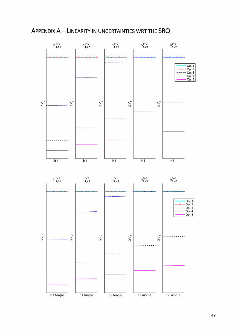
49
APPENDIX A – LINEARITY IN UNCERTAINTIES WRT THE SRQ

50

51

52

53

54
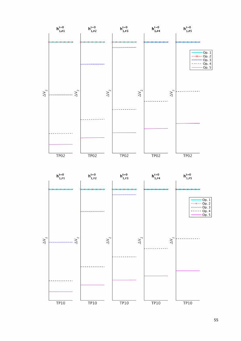
55