Investigating the performance of neural network … · Department of Physics and Electronics, Rhodes University, 6140, ... Correspondence to: J. B. Habarulema ([email protected])

Ann. Geophys., 30, 857–866, 2012www.ann-geophys.net/30/857/2012/doi:10.5194/angeo-30-857-2012© Author(s) 2012. CC Attribution 3.0 License.

AnnalesGeophysicae

Investigating the performance of neural network backpropagationalgorithms for TEC estimations using South African GPS data

J. B. Habarulema and L.-A. McKinnell

South African National Space Agency (SANSA), Space Science, 7200 Hermanus, South Africa

Department of Physics and Electronics, Rhodes University, 6140, Grahamstown, South Africa

Correspondence to:J. B. Habarulema ([email protected])

Received: 1 December 2011 – Revised: 26 March 2012 – Accepted: 2 May 2012 – Published: 24 May 2012

Abstract. In this work, results obtained by investigatingthe application of different neural network backpropaga-tion training algorithms are presented. This was done to as-sess the performance accuracy of each training algorithmin total electron content (TEC) estimations using identicaldatasets in models development and verification processes.Investigated training algorithms are standard backpropaga-tion (SBP), backpropagation with weight delay (BPWD),backpropagation with momentum (BPM) term, backpropa-gation with chunkwise weight update (BPC) and backprop-agation for batch (BPB) training. These five algorithms areinbuilt functions within the Stuttgart Neural Network Sim-ulator (SNNS) and the main objective was to find out thetraining algorithm that generates the minimum error betweenthe TEC derived from Global Positioning System (GPS) ob-servations and the modelled TEC data. Another investigatedalgorithm is the MatLab based Levenberg-Marquardt back-propagation (L-MBP), which achieves convergence after theleast number of iterations during training. In this paper, neu-ral network (NN) models were developed using hourly TECdata (for 8 years: 2000–2007) derived from GPS observa-tions over a receiver station located at Sutherland (SUTH)(32.38◦ S, 20.81◦ E), South Africa. Verification of the NNmodels for all algorithms considered was performed on both“seen” and “unseen” data. Hourly TEC values over SUTHfor 2003 formed the “seen” dataset. The “unseen” datasetconsisted of hourly TEC data for 2002 and 2008 over CapeTown (CPTN) (33.95◦ S, 18.47◦ E) and SUTH, respectively.The models’ verification showed that all algorithms investi-gated provide comparable results statistically, but differ sig-nificantly in terms of time required to achieve convergenceduring input-output data training/learning. This paper there-fore provides a guide to neural network users for choosing

appropriate algorithms based on the availability of computa-tion capabilities used for research.

Keywords. Ionosphere (Modelling and forecasting)

1 Introduction

Total electron content (TEC) estimations using the neuralnetwork (NN) technique have been done over many yearswith relative success (e.g.Hernandez-Pajares et al., 1997;Tulunay et al., 2004, 2006; Leandro and Santos, 2007; Senalpet al., 2008; Yilmaz et al., 2009). The main work in the ap-plication of this nonlinear technique involves finding a rela-tionship between known input and output parameters usinga relevant training algorithm. A training algorithm or learn-ing function has the purpose of adjusting connection weightsbetween input and output layers to achieve the desired resultfor the system under characterisation (Haykin, 1994; Rojas,1996; Zell et al., 1998). This study undertakes an investi-gation of some training algorithms employed in TEC mod-els by different research groups. Specifically, this is a com-parative study of performance levels of some algorithms forfeed forward networks only. Considered algorithms are back-propagation for batch (BPB) training, backpropagation withmomentum (BPM) term, backpropagation with chunkwiseweight update (BPC), backpropagation with weight delay(BPWD), standard backpropagation (SBP) and Levernberg-Marquardt backpropagation (L-MBP). The first five trainingalgorithms are inbuilt functions within the Stuttgart Neu-ral Network Simulator (SNNS) software (Zell et al., 1998;Reczko et al., 1998). The sixth algorithm implemented is aMatLab based L-MBP (Demuth et al., 2009).

Published by Copernicus Publications on behalf of the European Geosciences Union.

858 J. B. Habarulema and L.-A. McKinnell: Backpropagation training algorithms in TEC estimations

These algorithms mainly differ in the way that weightsare adjusted; otherwise, backpropagation is essentially im-plemented during training. Comprehensive details of thesealgorithms with mathematical descriptions of weight adjust-ments and procedure of their applications can be found inRojas(1996); Zell et al. (1998), andDemuth et al.(2009).For its simplicity, SBP algorithm has been widely used forTEC modelling and mapping in both feed forward and re-current neural networks (e.g.Leandro and Santos, 2007; Yil-maz et al., 2009; Habarulema et al., 2007, 2009, 2010). Re-search has shown that different problems require differenttraining algorithms and types of neural networks. For exam-ple, in space weather applications involving predictions thatuse solar wind data as inputs, recurrent networks have beenfound to be more desirable (Lundstedt et al., 2002; Weigelet al., 2002, 2003; Vandegriff et al., 2005; Lundestedt, 2006;Habarulema et al., 2009; Heilig et al., 2010). Other iono-spheric parameters, such as the critical frequency of the E-region (foE) and critical frequency of the F2 layer (foF2),have been predicted using feed forward networks (e.g.Can-der et al., 1998; Cander, 1998; McKinnell, 2002; McKinnelland Poole, 2004; Oyeyemi et al., 2006). Radial basis func-tion networks have also been used in the generation of TECdata for ionospheric TEC mapping, as well as short termforecasting offoF2 (e.g.Chan and Canon, 2002; Yilmazet al., 2009). TEC modelled and forecasted results for mod-els, which utilised the L-MBP algorithm, have also beenpresented (Tulunay et al., 2006; Yilmaz et al., 2009). Thisalgorithm is credited for its time savings during NN train-ing/learning processes (Jang et al., 1997). While neural net-works have been widely applied to ionospheric data, few re-sources are available which compare the performances of dif-ferent algorithms with specific emphasis on ionospheric pa-rameter modelling. Although this paper does not investigateall training algorithms, it serves as a guide to neural networkusers who may want to apply different training algorithms totheir datasets, especially for ionospheric applications.

NN models are developed using a similar dataset with dif-ferent training algorithms and verified on statistically simi-lar (not necessarily identical) datasets (both “seen” and “un-seen”) to assess their performance levels. Training was doneon a 2.4 GHz PC with 2 GB RAM. For fair comparisons, thesame architecture – comprised of one input layer (6 inputnodes), one hidden layer (9 hidden nodes) and one outputlayer – was used. In this way, it has been observed that thenumber of epochs/iterations required to achieve convergenceor generalisation is the main determinant in the choice ofthe algorithm, especially for time needed and computing ca-pability available. Table 1 shows the approximate time anditerations determined for each algorithm to achieve conver-gence. BPB has the highest number of iterations and hencetakes longer to give the optimum solution. This may be re-lated to the learning rate, which contributes to the “speed”with which training takes place. In BPB, the learning param-eter is divided by the number of training patterns, making

Table 1.Approximate number of iterations and time taken (in min-utes) for generalisation to be achieved for different training algo-rithms.

Training Number of Approximate time (minutes)algorithm iterations for convergence

BPB 16 800 18.5SBP 3500 4.3BPC 2400 2.933BPM 1000 1.1BPWD 1000 1.2667L-MBP 165 3

it significantly small, and it could therefore slow the train-ing rate of the network on all training patterns (Zell et al.,1998). Results discussed in this paper were obtained fromNN models developed using the South African data fromthe Sutherland station (SUTH) (32.38◦ S, 20.81◦ E) hourly(1–23 h) TEC dataset (2000–2007) of∼50 300 data points,which accounted for∼74.87 % derivable data for the pe-riod considered. The verification was done on 2003 and 2008datasets over SUTH, as well as the 2002 dataset over CapeTown (CPTN), South Africa (33.95◦ S, 18.47◦ E).

2 Data

2.1 TEC from GPS

GPS TEC data were derived from observations made bydual frequency receivers located at SUTH and CPTN, bothin South Africa. The values were derived using the ad-justed spherical harmonic analysis (ASHA) algorithm, whichmakes use of the mapping function that assumes the iono-sphere to be a single layer of height 350 km (Opperman et al.,2007). A total of 9 years (2000–2008) of data was derivedover SUTH, of which the 2000–2007 dataset was utilised inthe development of the NN models. Hourly TEC data for2008 was used in the final verification of the models alongwith CPTN data for the year 2002. The ASHA algorithmis based on spherical harmonic expansion and was adaptedfrom theSchaer(1999) global model to be used as a regionalmodel. It uses data from a local GPS receiver network andwas chosen to estimate single station TEC results for com-parative purposes with ionosonde measurements (Oppermanet al., 2007). Full details of the TEC derivation procedurefrom GPS observations using the ASHA algorithm (and itsvalidation with different data sources) are presented inOp-perman et al.(2007) andOpperman(2007).

2.2 Physical and geophysical data parameters

TEC is modelled as a function of known physical and geo-physical parameters which influence its variability. These areseasonal and diurnal variations, as well as solar activity and

Ann. Geophys., 30, 857–866, 2012 www.ann-geophys.net/30/857/2012/

J. B. Habarulema and L.-A. McKinnell: Backpropagation training algorithms in TEC estimations 859

geomagnetic activity. Seasonal and diurnal variations are ef-fectively represented by day number of the year (DOY) andhour of the day (HOD), respectively. The measure of the solaractivity is represented by the sunspot number, while the mag-netic A index values account for the geomagnetic influenceon TEC. Quantitatively, the magnetic and solar activities de-termined byHabarulema et al.(2007) for South African GPSTEC modelling were used in this study. These are the aver-age of the previous 4-months for the daily sunspot numberand the average of the previous eight 3-hourly magnetic Aindex values (A8) derived from the archived K-index datarecorded at the Hermanus Magnetic Observatory (34.43◦ S,19.23◦ E), South Africa. Diurnal and seasonal variation rep-resentations, sunspot number, and geographic latitudes andlongitudes have been used previously in the modelling offoF2 and TEC using neural networks (e.g.Cander et al.,1998; McKinnell, 2002; McKinnell and Poole, 2004; Lean-dro and Santos, 2007).

3 Selected functions required for training

Data representations for parameters which influence TECvariability along with known TEC values make up the train-ing patterns of the form[(x1, t1), (x2, t2), ..., (xn, tn)], wherexi is the training pattern consisting of inputs, andti is thetarget corresponding toxi (where i = 1,2, ...,n). The up-date and initialisation functions used for BPB, BPC, BPM,BPWD and SBP algorithms are topological order and ran-domised weights, respectively. The initialisation functionrandomly selects the weights which are real numbers. Pre-senting an input patternxi from the training set generates anoutputoi which is different from the target outputti . The aimis to ensure thatoi andti are identical fori = 1,2, ...,n withthe help of a training/learning algorithm (Haykin, 1994; Ro-jas, 1996; Zell et al., 1998); the ultimate goal is to minimisethe error function of the network defined as

Nne =1

2

n∑i=1

(oi − ti)2 (1)

whereNne is the error function of the network.OnceNne has been sufficiently minimised for the train-

ing dataset, input patterns not known to the network are pre-sented, and the network is expected to recognise whether thenew input patterns are similar to the learned patterns. Oncethis condition is met, the network generates a similar out-put (Rojas, 1996). This interpolation process is the one re-ferred to as the verification of the NN models. Therefore,training/learning involves finding the optimal combinationof weights that allows the network function to approximatea given function, in this case implicitly through known in-put and target training examples (Rojas, 1996). Topologicalorder update simply means that the presented input trainingpattern propagates forward from the input layer through thehidden layer until the activation reaches the output layer (Zell

Table 2.Computed correlation coefficient values for SUTH in 2003.

Training Correlation coefficients at different times (UT)

algorithm all hours 04:00 10:00 16:00 22:00

BPB 0.9229 0.7636 0.6898 0.8400 0.7393BPC 0.9303 0.7834 0.7180 0.8468 0.5995BPM 0.9309 0.7876 0.7219 0.8535 0.6202BPWD 0.9309 0.7876 0.7219 0.8535 0.6202SBP 0.9312 0.7954 0.7178 0.8516 0.5940L-MBP 0.9381 0.8470 0.7407 0.8615 0.7662

et al., 1998). No pattern remap function was used. The pur-pose of a pattern remap function is to quickly vary the desiredoutput of the network without changing the pattern files dur-ing training, and non-use indicates that no remapping wasdone and thus all presented patterns were trained (Zell et al.,1998; Reczko et al., 1998). In the implementation of thesefunctions, a similar network setup of 6 input nodes, 9 hid-den nodes and 1 output node was used during the training ofthe network. The same architecture was used for the L-MBPalgorithm.

4 Results and discussion

4.1 Interpolation results

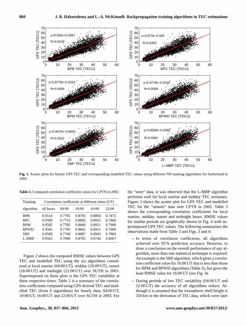
It is known that neural networks interpolate well within theinput space, and therefore the network is expected to repro-duce the dataset that was used to train it with relatively goodaccuracy (McKinnell, 2002; Habarulema et al., 2007). Sincethe main aim is to compare the performance accuracies ofthe training algorithms on the training dataset, part of thetraining dataset can still be used in the final verification ofthe models. This can be referred to as the determination ofthe correct application of the neural network technique ona particular dataset. The overall verification of the modelswas performed using Sutherland (2003 and 2008) and CapeTown (2002) datasets. While it is expected that the networkshould perform very well for SUTH 2003 data (part of thetraining dataset), the differences between algorithm perfor-mances should be evident if present. Figure 1 shows the scat-ter plot for hourly GPS TEC and modelled TEC values usingdifferent NN training algorithms over SUTH for 2003. Cor-relation coefficient values indicate a slightly better perfor-mance by the L-MBP algorithm compared to the rest of theconsidered algorithms. The widely used algorithms (SBP andL-MBP) in ionospheric modelling provide improved interpo-lation of TEC estimates. Although the model was tested onthe “seen” dataset (2003), it was noted that all training algo-rithms achieved over 90 % accuracy (over the entire dataset,denoted as “all hours” in Table 2) in estimating TEC, andtheir modelling results are highly comparable.

www.ann-geophys.net/30/857/2012/ Ann. Geophys., 30, 857–866, 2012


0 10 20 30 40 50 600

10203040506070

GP

S T

EC

(T

EC

U)

BPB TEC (TECU)

y=0.935x+0.3567

R=0.9229

0 10 20 30 40 50 600

10203040506070

GP

S T

EC

(T

EC

U)

BPC TEC (TECU)

y=0.973x−0.405

R=0.9303

0 10 20 30 40 50 600

10203040506070

GP

S T

EC

(T

EC

U)

BPM TEC (TECU)

y=0.9778x−0.2034

R=0.9309

0 10 20 30 40 50 600

10203040506070

GP

S T

EC

(T

EC

U)

BPWD TEC (TECU)

y=0.9778x−0.2034

R=0.9309

0 10 20 30 40 50 600

10203040506070

GP

S T

EC

(T

EC

U)

SBP TEC (TECU)

y=0.9676x−0.6565

R=0.9312

0 10 20 30 40 50 600

10203040506070

GP

S T

EC

(T

EC

U)

L−MBP TEC (TECU)

y=0.9638x−0.0285

R=0.9381

Fig. 1. Scatter plots for hourly GPS TEC and corresponding modelled TEC values using different NN training algorithms for Sutherland in2003.

Table 3.Computed correlation coefficient values for CPTN in 2002.

Training Correlation coefficients at different times (UT)

algorithm all hours 04:00 10:00 16:00 22:00

BPB 0.9514 0.7705 0.8705 0.8804 0.7475BPC 0.9589 0.7733 0.8885 0.8925 0.7866BPM 0.9585 0.7785 0.8840 0.8951 0.7900BPWD 0.9585 0.7785 0.8841 0.8951 0.7900SBP 0.9589 0.7768 0.8887 0.8943 0.7883L-MBP 0.9563 0.7896 0.8785 0.8744 0.8067

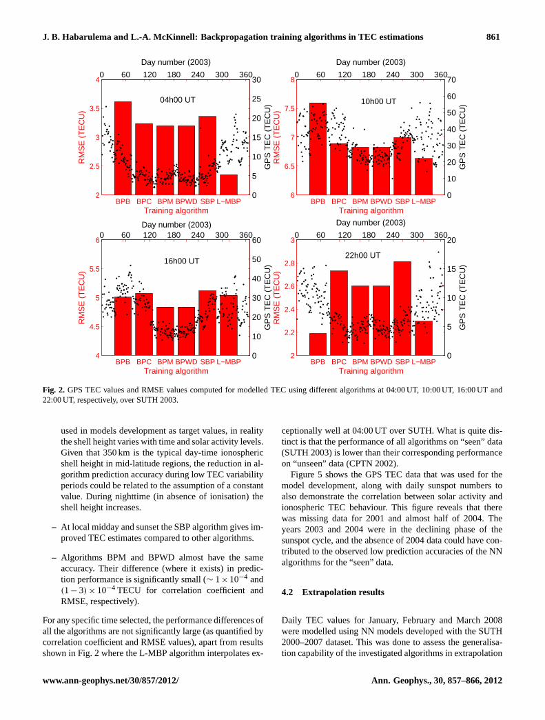
Figure 2 shows the computed RMSE values between GPSTEC and modelled TEC using the six algorithms consid-ered at local sunrise (04:00 UT), midday (10:00 UT), sunset(16:00 UT) and midnight (22:00 UT) over SUTH in 2003.Superimposed on these plots is the GPS TEC variability atthese respective times. Table 2 is a summary of the correla-tion coefficients computed using GPS derived TEC and mod-elled TEC (from 6 algorithms) for hourly data, 04:00 UT,10:00 UT, 16:00 UT and 22:00 UT over SUTH in 2003. For

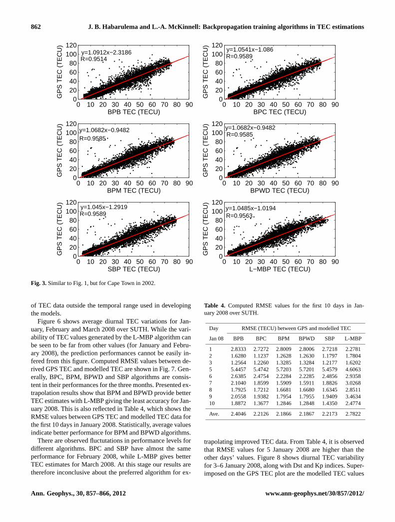
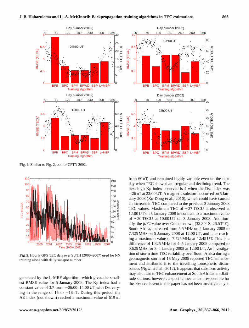
the “seen” data, it was observed that the L-MBP algorithmperforms well for local sunrise and midday TEC estimates.Figure 3 shows the scatter plot for GPS TEC and modelledTEC for the “unseen” data over CPTN in 2002. Table 3shows the corresponding correlation coefficients for localsunrise, midday, sunset and midnight hours. RMSE valuesfor similar periods are graphically shown in Fig. 4 with su-perimposed GPS TEC values. The following summarises theobservations made from Table 3 and Figs. 3 and 4:

– In terms of correlation coefficients, all algorithmsachieved over 95 % prediction accuracy. However, todraw a conclusion on the overall performance of any al-gorithm, more than one statistical technique is required.An example is the SBP algorithm, which gives a correla-tion coefficient value for 16:00 UT that is less than thosefor BPM and BPWD algorithms (Table 3), but gives theleast RMSE value for 16:00 UT (see Fig. 4).

– During periods of low TEC variability (04:00 UT and22:00 UT) the accuracy of all algorithms reduce. Al-though it is assumed that the ionospheric shell height is350 km in the derivation of TEC data, which were later



BPB BPC BPM BPWD SBP L−MBP2

2.5

3

3.5

4R

MS

E (

TE

CU

)

Training algorithm

0 60 120 180 240 300 360

0

5

10

15

20

25

30

GP

S T

EC

(T

EC

U)

Day number (2003)

04h00 UT


6.5

7

7.5

8

RM

SE

(T

EC

U)

Training algorithm

0 60 120 180 240 300 360

0

10

20

30

40

50

60

70

GP

S T

EC

(T

EC

U)

Day number (2003)

10h00 UT


4.5

5

5.5

6

RM

SE

(T

EC

U)

Training algorithm

0 60 120 180 240 300 360

0

10

20

30

40

50

60

GP

S T

EC

(T

EC

U)

Day number (2003)

16h00 UT


2.2

2.4

2.6

2.8

3

RM

SE

(T

EC

U)

Training algorithm

0 60 120 180 240 300 360

0

5

10

15

20

GP

S T

EC

(T

EC

U)

Day number (2003)

22h00 UT

Fig. 2. GPS TEC values and RMSE values computed for modelled TEC using different algorithms at 04:00 UT, 10:00 UT, 16:00 UT and22:00 UT, respectively, over SUTH 2003.

used in models development as target values, in realitythe shell height varies with time and solar activity levels.Given that 350 km is the typical day-time ionosphericshell height in mid-latitude regions, the reduction in al-gorithm prediction accuracy during low TEC variabilityperiods could be related to the assumption of a constantvalue. During nighttime (in absence of ionisation) theshell height increases.

– At local midday and sunset the SBP algorithm gives im-proved TEC estimates compared to other algorithms.

– Algorithms BPM and BPWD almost have the sameaccuracy. Their difference (where it exists) in predic-tion performance is significantly small (∼ 1×10−4 and(1− 3) × 10−4 TECU for correlation coefficient andRMSE, respectively).

For any specific time selected, the performance differences ofall the algorithms are not significantly large (as quantified bycorrelation coefficient and RMSE values), apart from resultsshown in Fig. 2 where the L-MBP algorithm interpolates ex-

ceptionally well at 04:00 UT over SUTH. What is quite dis-tinct is that the performance of all algorithms on “seen” data(SUTH 2003) is lower than their corresponding performanceon “unseen” data (CPTN 2002).

Figure 5 shows the GPS TEC data that was used for themodel development, along with daily sunspot numbers toalso demonstrate the correlation between solar activity andionospheric TEC behaviour. This figure reveals that therewas missing data for 2001 and almost half of 2004. Theyears 2003 and 2004 were in the declining phase of thesunspot cycle, and the absence of 2004 data could have con-tributed to the observed low prediction accuracies of the NNalgorithms for the “seen” data.

4.2 Extrapolation results

Daily TEC values for January, February and March 2008were modelled using NN models developed with the SUTH2000–2007 dataset. This was done to assess the generalisa-tion capability of the investigated algorithms in extrapolation



0 10 20 30 40 50 60 70 80 900

20406080

100120

GP

S T

EC

(T

EC

U)

BPB TEC (TECU)

y=1.0912x−2.3186R=0.9514

0 10 20 30 40 50 60 70 80 900

20406080

100120

GP

S T

EC

(T

EC

U)

BPC TEC (TECU)

y=1.0541x−1.086R=0.9589

0 10 20 30 40 50 60 70 80 900

20406080

100120

GP

S T

EC

(T

EC

U)

BPM TEC (TECU)

y=1.0682x−0.9482R=0.9585

0 10 20 30 40 50 60 70 80 900

20406080

100120

GP

S T

EC

(T

EC

U)

BPWD TEC (TECU)

y=1.0682x−0.9482R=0.9585

0 10 20 30 40 50 60 70 80 900

20406080

100120

GP

S T

EC

(T

EC

U)

SBP TEC (TECU)

y=1.045x−1.2919R=0.9589

0 10 20 30 40 50 60 70 80 900

20406080

100120

GP

S T

EC

(T

EC

U)

L−MBP TEC (TECU)

y=1.0485x−1.0194R=0.9563

Fig. 3.Similar to Fig. 1, but for Cape Town in 2002.

of TEC data outside the temporal range used in developingthe models.

Figure 6 shows average diurnal TEC variations for Jan-uary, February and March 2008 over SUTH. While the vari-ability of TEC values generated by the L-MBP algorithm canbe seen to be far from other values (for January and Febru-ary 2008), the prediction performances cannot be easily in-fered from this figure. Computed RMSE values between de-rived GPS TEC and modelled TEC are shown in Fig. 7. Gen-erally, BPC, BPM, BPWD and SBP algorithms are consis-tent in their performances for the three months. Presented ex-trapolation results show that BPM and BPWD provide betterTEC estimates with L-MBP giving the least accuracy for Jan-uary 2008. This is also reflected in Table 4, which shows theRMSE values between GPS TEC and modelled TEC data forthe first 10 days in January 2008. Statistically, average valuesindicate better performance for BPM and BPWD algorithms.

There are observed fluctutations in performance levels fordifferent algorithms. BPC and SBP have almost the sameperformance for February 2008, while L-MBP gives betterTEC estimates for March 2008. At this stage our results aretherefore inconclusive about the preferred algorithm for ex-

Table 4. Computed RMSE values for the first 10 days in Jan-uary 2008 over SUTH.

Day RMSE (TECU) between GPS and modelled TEC

Jan 08 BPB BPC BPM BPWD SBP L-MBP

1 2.8333 2.7272 2.8009 2.8006 2.7218 2.27812 1.6280 1.1237 1.2628 1.2630 1.1797 1.78043 1.2564 1.2260 1.3285 1.3284 1.2177 1.62025 5.4457 5.4742 5.7203 5.7201 5.4579 4.60636 2.6385 2.4754 2.2284 2.2285 2.4856 2.93587 2.1040 1.8599 1.5909 1.5911 1.8826 3.02688 1.7925 1.7212 1.6681 1.6680 1.6345 2.85119 2.0558 1.9382 1.7954 1.7955 1.9409 3.463410 1.8872 1.3677 1.2846 1.2848 1.4350 2.4774

Ave. 2.4046 2.2126 2.1866 2.1867 2.2173 2.7822

trapolating improved TEC data. From Table 4, it is observedthat RMSE values for 5 January 2008 are higher than theother days’ values. Figure 8 shows diurnal TEC variabilityfor 3–6 January 2008, along with Dst and Kp indices. Super-imposed on the GPS TEC plot are the modelled TEC values




4.5

5

5.5

6R

MS

E (

TE

CU

)

Training algorithm

0 60 120 180 240 300 360

0

5

10

15

20

25

30

GP

S T

EC

(T

EC

U)

Day number (2002)

04h00 UT


8.5

9

9.5

10

RM

SE

(T

EC

U)

Training algorithm

0 60 120 180 240 300 360

0

20

40

60

80

GP

S T

EC

(T

EC

U)

Day number (2002)

10h00 UT


7.5

8

8.5

9

RM

SE

(T

EC

U)

Training algorithm

0 60 120 180 240 300 360

0

20

40

60

80

GP

S T

EC

(T

EC

U)

Day number (2002)

16h00 UT


3.5

4

4.5

5

RM

SE

(T

EC

U)

Training algorithm

0 60 120 180 240 300 360

0

5

10

15

20

25

30

GP

S T

EC

(T

EC

U)

Day number (2002)

22h00 UT

Fig. 4.Similar to Fig. 2, but for CPTN 2002.

2000 2001 2002 2003 2004 2005 2006 20070

10

20

30

40

50

60

70

80

90

100

110

TE

C (

TE

CU

)

Time (2000−2007)

0

20

40

60

80

100

120

140

160

180

200

220

240

Sun

spot

num

ber

Fig. 5.Hourly GPS TEC data over SUTH (2000–2007) used for NNtraining along with daily sunspot number.

generated by the L-MBP algorithm, which gives the small-est RMSE value for 5 January 2008. The Kp index had aconstant value of 3.7 from∼06:00–14:00 UT with Dst vary-ing in the range of 15 to−18 nT. During this period, theAE index (not shown) reached a maximum value of 619 nT

from 60 nT, and remained highly variable even on the nextday when TEC showed an irregular and declining trend. Thenext high Kp index observed is 4 when the Dst index was−26 nT at 23:00 UT. A magnetic substorm occurred on 5 Jan-uary 2008 (Xu-Dong et al., 2010), which could have causedan increase in TEC compared to the previous 3 January 2008TEC values. Maximum TEC of∼27 TECU is observed at12:00 UT on 5 January 2008 in contrast to a maximum valueof ∼20 TECU at 10:00 UT on 3 January 2008. Addition-ally, thefoF2 value over Grahamstown (33.30◦ S, 26.53◦ E),South Africa, increased from 5.5 MHz on 4 January 2008 to7.325 MHz on 5 January 2008 at 12:00 UT, and later reach-ing a maximum value of 7.725 MHz at 12:45 UT. This is adifference of 1.825 MHz for 4–5 January 2008 compared to0.625 MHz for 3–4 January 2008 at 12:00 UT. An investiga-tion of storm time TEC variability over South Africa during ageomagnetic storm of 15 May 2005 reported TEC enhance-ment and attributed it to the travelling ionospheric distur-bances (Ngwira et al., 2012). It appears that substorm activitymay also lead to TEC enhancement at South African midlati-tude stations; however, a specific mechanism responsible forthe observed event in this paper has not been investigated yet.



0

5

10

15

20

January 2008

(a)

BPB BPC BPM BPWD SBP L−MBP GPS

0

5

10

15

February 2008

(b)

0 2 4 6 8 10 12 14 16 18 20 22 240

5

10

15

March 2008

Time (UT)

Mod

elle

d or

GP

S T

EC

(T

EC

U)

(c)

Fig. 6.Hourly average modelled and GPS TEC values for January, February and March 2008 over SUTH.

0

1

2

3

January 2008

0

1

2

3

February 2008


1

2

3

Training algorithm

RM

SE

(T

EC

U)

March 2008

Fig. 7.RMSE values for January, February and March 2008.

5 Conclusions

This paper has presented results comparing performance lev-els of some backpropagation algorithms for ionospheric TECestimations. Similar to other sources (e.g.Jang et al., 1997;

4 8 121620 0 4 8 121620 0 4 8 121620 0 4 8 121620 00

10

20

30

TE

C (

TE

CU

)

03 Jan 2008 04 Jan 2008 05 Jan 2008 06 Jan 2008

GPS TECL−MBP TEC

4 8 121620 0 4 8 121620 0 4 8 121620 0 4 8 121620 00123456789

Kp

Time (UT)4 8 121620 0 4 8 121620 0 4 8 121620 0 4 8 121620 0

−30−20−10010203040

Dst

(nT

)

Fig. 8. Diurnal TEC values for 3–6 January 2008. Dst and Kp in-dices for this period are also shown.

Yilmaz et al., 2009), it is evident that the L-MBP algorithmrequires the fewest number of iterations, compared to otheralgorithms, to achieve generalisation. The reported conver-gence time (∼3 min) is expected to reduce with improvedcomputing capacity. For TEC modelling, the differences inaccuracy between the investigated algorithms is not very sig-nificant. What is worth noting, though, is the time it takes



each algorithm to achieve convergence or generalisation.This time can increase or decrease depending on the size ofthe dataset under consideration. This investigation was con-ducted using a dataset of∼50 300 data points. Each algo-rithm can generally be used depending on user requirementsand available resources. For small datasets, the MatLab basedL-MBP algorithm is sufficient. With more computing power,the other training algorithms can be used to slightly improvethe accuracy. BPM and BPWD algorithms appear to achievethe same accuracy in a relatively short period of time andmay be advantageous over the SBP algorithm, which hasbeen widely used for modelling various ionospheric parame-ters. According toZell et al.(1998), the momentum term (inthe BPM) leads to the computation of the new weight changeusing the old weight change (during training), thereby mim-imising oscillations associated with SBP for narrow mini-mum area error surfaces. BPM is a simple modification ofSBP which accelerates the training/learning process (Rojas,1996), and this is clearly evident in Table 1 in terms of thetime and number of epochs required to achieve convergence.

Acknowledgements.J. B. Habarulema’s research is supported bythe South African National Space Agency (SANSA) and NationalResearch Foundation (NRF), South Africa. The GPS data was pro-vided by the Chief Directorate: National Geo-spatial information,South Africa.

Topical Editor K. Kauristie thanks two anonymous referees fortheir help in evaluating this paper.

References

Cander, L. R.: Artificial neural network applications in ionosphericstudies, Annali De Geofisica, 5–6, 757–766, 1998.

Cander, L. R., Milosavljevic, M. M., Stankovic, S. S., and Toma-sevic, S.: Ionospheric forecasting technique by artificial neuralnetwork, Electronic letters, 34, 1573–1574, 1998.

Chan, A. H. Y. and Cannon, P. S.: Nonlinear forecasts offoF2: vari-ation of model predictive accuracy over time, Ann. Geophys., 20,1031–1038,doi:10.5194/angeo-20-1031-2002, 2002.

Demuth, H., Beale, M., and Hagan, M.: Neural Networkbox Box™

6 User’s Guide, The MathWorks™, 2009.Habarulema, J. B., McKinnell, L. A., and Cilliers, P. J.: Prediction

of global positioning system total electron content using neu-ral networks over South Africa, J. Atmos Solar Terr. Phys., 69,1842–1850, 2007.

Habarulema, J. B., McKinnell, L.-A., and Opperman, B. D. L.:A recurrent neural network approach to quantitatively study-ing solar wind effects on TEC derived from GPS; preliminaryresults, Ann. Geophys., 27, 2111–2125,doi:10.5194/angeo-27-2111-2009, 2009.

Habarulema, J. B., McKinnell, L.-A., and Opperman, B. D. L.: TECmeasurements and modelling over Southern Africa during mag-netic storms; a comparative analysis, J. Atmos. Solar Terr. Phys.,72, 509–520, 2010.

Haykin, S.: Neural Networks, A Comprehensive Foundation,Macmillan College Publishing Company, 1994.

Heilig, B., Lotz, S., Vero, J., Sutcliffe, P., Reda, J., Pajunpaa, K., andRaita, T.: Empirically modelled Pc3 activity based on solar windparameters, Ann. Geophys., 28, 1703–1722,doi:10.5194/angeo-28-1703-2010, 2010.

Hernandez-Pajares, M., Juan, J., and Sanz, J.: Neural network mod-elling of the ionospheric electron content at global scale usingGPS, Radio Sci., 32, 1081–1090, 1997.

Jang, J. S. R., Sun, C. T., and Mizutani, E.: Neuro Fuzzy andSoft Computing, Prentice-Hall, Upper Saddle River, New Jersey,1997.

Leandro, R. F. and Santos, M. C.: A neural network approach forregional vertical total electron content modelling, Studia Geo-physica et Geodaetica, 51, 279–292, 2007.

Lundestedt, H.: Solar activity modelled and forecasted: A new ap-proach, Adv. Space Res., 38, 862–867, 2006.

Lundstedt, H., Gleisner, and Wintoft, P.: Operational forecastsof the geomagnetic Dst index, Geophys. Res. Lett., 29, 2181,doi:10.1029/2002GL016151, 2002.

McKinnell, L.-A.: A Neural Network based Ionospheric model forthe bottomside electron density profile over Grahamstown, SouthAfrica, Ph.D. thesis of Rhodes University, Grahamstown, SouthAfrica, 2002.

McKinnell, L.-A. and Poole, A. W. V.: Predicting the ionosphericF layer using neural networks, J. Geophys. Res., 109, A08308,doi:10.1029/2004JA010445, 2004.

Ngwira, C. M., McKinnell, L.-A., Cilliers, P. J., and Yizengaw, E.:An investigation of ionospheric disturbances over South Africaduring the magnetic storm on 15 May 2005, Adv. Space Res.,49, 327–335, 2012.

Opperman, B.: Reconstructing Ionospheric TEC over South Africausing signals from a Regional GPS network, PhD thesis RhodesUniversity, Grahamstown, South Africa, 2007.

Opperman, B. D. L., Cilliers, P. J., McKinnell, L. A., and Hag-gard, R.: Development of a regional GPS-based ionospheric TECmodel for South Africa, Adv. Space Res., 39, 808–815, 2007.

Oyeyemi, E. O., McKinnell, L.-A., and Poole, A. W. V.: Near-real timefoF2 predictions using neural networks, J. Atmos. andSolar-Terr. Phys., 68, 1807–1818, 2006.

Reczko, M., Riedmiller, M., Seemann, M., Ritt, M., DeCoster, J.,Biedermann, J., Danz, J., Wehrfritz, C., Werner, R., Berthold, M.,and Orsier, B.: External contributions to Stuttgart Neural Net-work Simulator (SNNS), User Manual, Version 4.2, Universitiesof Stuttgart and Tubingen, Germany, and the European ParticleResearch Lab, CERN, Geneva, Switzerland, 1998.

Rojas, R.: Neural Networks – A Systematic Introduction, Springer-Verlag, Berlin, Germany, New-York, USA, 1996.

Schaer, S.: Mapping and Predicting the Earth’s Ionosphere Usingthe Global Positioning System, Ph.D. thesis, Astronomical Insti-tute, University of Berne, Berne Switzerland, 1999.

Senalp, E. T., Tulunay, E., and Tulunay, Y.: Total electroncontent (TEC) forecasting by Cascade Modeling, A possi-ble alternative to the IRI-2001, Radio Sci., 43, RS4016,doi:10.1029/2007RS003719, 2008.

Tulunay, E., Senalp, E. T., Cander, L. R., Tulunay, Y. K., Bilge,A. H., Mizrahi, E., Kouris, S. S., and Jakowski, N.: Developmentof algorithms and software for forecasting, nowcasting and vari-ability of TEC, Ann. Geophys., 47, 1201–1214, 2004.

Tulunay, E., Senalp, E., Radicella, S., and Tulunay, Y.: Forecastingtotal electron content maps by neural network technique, Radio


http://dx.doi.org/10.5194/angeo-20-1031-2002





http://dx.doi.org/10.1029/2002GL016151

http://dx.doi.org/10.1029/2004JA010445

http://dx.doi.org/10.1029/2007RS003719


Sci., 41, RS4016,doi:10.1029/2005RS003285, 2006.Vandegriff, J., Wagstaff, K., and G. Ho, J. P.: Forecasting space

weather: Predicting interplanetary shocks using neural networks,Adv. Space Res., 36, 2323–2327, 2005.

Weigel, R. S., Vassiliadis, D., and Klimas, A. J.: Coupling of the so-lar wind to temporal fluctuations in ground magnetic fields, Geo-phys. Res. Lett., 29, 1915,doi:10.1029/2002GL014740, 2002.

Weigel, R. S., Klimas, A. J., and Vassiliadis, D.: Solar windcoupling to and predictability of ground magnetic fieldsand their time derivatives, J. Geophys. Res., 108, 1298,doi:10.1029/2002JA009627, 2003.

Xu-Dong, Z., Ai-Min, D., Wen-Yao, X., Yuan, W., and Hao, L.:A near Earth reconnection of the magnetospheric substorm onJanuary 5, 2008: THEMIS observations, Chinese J. Geophys.,53, 1019–1027, 2010.

Yilmaz, A., Akdogan, K. E., and Gurun, M.: Regional TECmapping using neural networks, Radio Sci., 44, RS3007,doi:10.1029/2008RS004049, 2009.

Zell, A., Mamier, G. M., Vogt, M., Mache, N., Hubner, R., Doring,S., Herrmann, K.-U., Soyez, T., Schmalzl, M., Sommer, T.,Hatzigeorgiou, A., Posselt, D., Schreiner, T., Kett, B., Clemente,G., Wieland, J., and Gatter, J.: Stuttgart Neural Network Simula-tor (SNNS), User Manual, Version 4.2, Universities of Stuttgartand Tubingen, Germany, and the European Particle ResearchLab, CERN, Geneva, Switzerland, 1998.


http://dx.doi.org/10.1029/2005RS003285

http://dx.doi.org/10.1029/2002GL014740

http://dx.doi.org/10.1029/2002JA009627

http://dx.doi.org/10.1029/2008RS004049

Documents

Investigating the performance of neural network … · Department of Physics and Electronics, Rhodes University, 6140, ... Correspondence to: J. B. Habarulema ([email protected])