University of South Florida University of South Florida

Digital Commons @ University of South Florida Digital Commons @ University of South Florida

Graduate Theses and Dissertations Graduate School

June 2020

Investigating the Isotope Signatures of Dissolved Iron in the Investigating the Isotope Signatures of Dissolved Iron in the

Southern Atlantic Ocean Southern Atlantic Ocean

Brent A. Summers University of South Florida

Follow this and additional works at: https://digitalcommons.usf.edu/etd

Part of the Geochemistry Commons, and the Other Oceanography and Atmospheric Sciences and

Meteorology Commons

Scholar Commons Citation Scholar Commons Citation Summers, Brent A., "Investigating the Isotope Signatures of Dissolved Iron in the Southern Atlantic Ocean" (2020). Graduate Theses and Dissertations. https://digitalcommons.usf.edu/etd/9000

This Thesis is brought to you for free and open access by the Graduate School at Digital Commons @ University of South Florida. It has been accepted for inclusion in Graduate Theses and Dissertations by an authorized administrator of Digital Commons @ University of South Florida. For more information, please contact scholarcommons@usf.edu.

Investigating the Isotope Signatures of Dissolved Iron in the Southern Atlantic Ocean

by

Brent A. Summers

A thesis submitted in partial fulfillment of the requirements for the degree of Master of Science in Marine Science

with a concentration in Chemical Oceanography College of Marine Science University of South Florida

Major Professor: Tim Conway, Ph.D. Robert Byrne, Ph.D.

William Homoky, Ph.D.

Date of Approval: June 19, 2020

Keywords: trace metal, biogeochemistry, sediments, GEOTRACES, Río de la Plata, Southern Ocean

Copyright © 2020, Brent A. Summers

ACKNOWLEDGMENTS

I would first like to thank my advisor, Tim Conway, for allowing me the opportunity to

join his lab and pursue a Master’s degree. His guidance and support throughout the last three years

not only helped me become a better scientist, but also a better person. I would also like to thank

my lab mates, Matthias and Zach, for providing me with feedback on my defense presentation and

for being such great friends over the last year. I would like to thank Peter Morton, Jenny, and the

kids for providing me with a science- and fun-filled time while completing my undergraduate

degree at Florida State University. I would like to thank my Mom, Dad, and my brother, Chad, for

the endless encouragement throughout my life. Thank you to my girlfriend, Lea, and my step-dog,

Gia, for always loving me and pushing (or pulling) me along. I wouldn’t have been able to achieve

this without funding from the Anne and Werner Von Rosenstiel Fellowship in Marine Science.

Lastly, thank you to the countless friends and family throughout my life who have encouraged me.

All your support helped me achieve this goal.

i

TABLE OF CONTENTS List of Tables ................................................................................................................................. ii List of Figures ................................................................................................................................ iii Abstract ......................................................................................................................................... iv Chapter One: Introduction ..............................................................................................................1

1.1 Importance of Iron as a Nutrient ...................................................................................1 1.2 Sources of Iron to the Ocean ..........................................................................................3 1.3 Iron Stable Isotopes and Source Signatures ..................................................................4 1.4 Sediment Iron Isotope Cycling Questions .....................................................................6 1.5 Research Overview ........................................................................................................9 1.6 South Atlantic Oceanographic Setting and Regional Iron Cycling ............................10

Chapter Two: Methods ..................................................................................................................17 2.1 Sample Collection .......................................................................................................17 2.2 Clean Laboratory Procedures .......................................................................................17 2.3 Chemical Methods ......................................................................................................18 2.3.1 Extraction from Seawater Matrix ..................................................................19 2.3.2 Trace Metal Purification ..............................................................................19 2.4 Analytical Methods .....................................................................................................20 Chapter Three: Results and Discussion ........................................................................................23 3.1 Procedural Blanks .......................................................................................................23 3.2 Precision and Accuracy ................................................................................................23 3.3 GA10W Results ..........................................................................................................24 3.3.1 GA10W Margin Stations 22 and 24 ..............................................................25 3.3.2 GA10W Surface Transect ............................................................................26 3.4 GA10W Discussion ....................................................................................................28 3.4.1 Shelf and Slope Sediment Isotope Signature and Influence .........................28 3.4.2 Fe Sources in Western Surface Waters and the Influence of the Río de la Plata .........................................................................................................31 3.4.3 Biological Cycling of Fe Isotopes South of the SSTC .................................34 3.4.4 Sediment Supply from the African Margin .................................................35 Chapter Four: Conclusions ............................................................................................................45 References ......................................................................................................................................47

ii

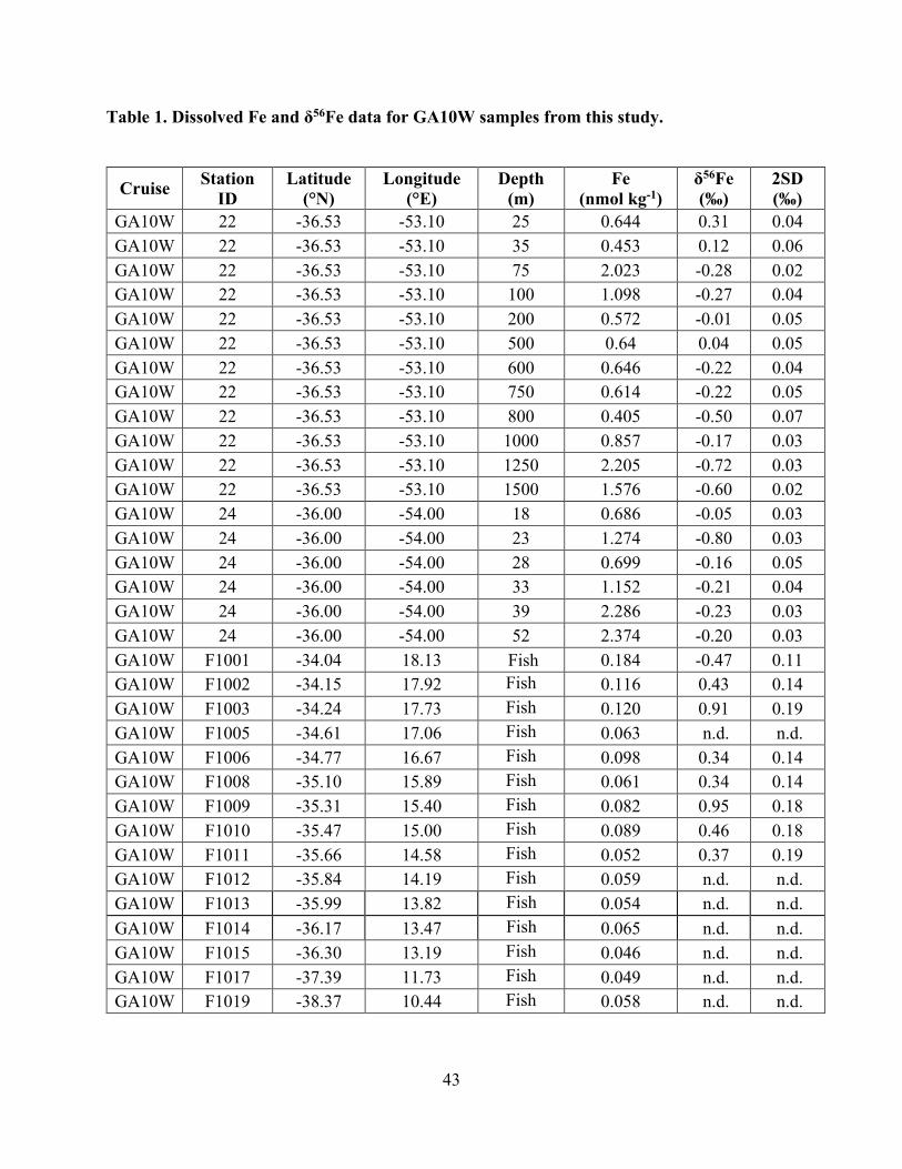
LIST OF TABLES Table 1: Dissolved Fe and δ56Fe data for GA10W samples from this study .............................43

iii

LIST OF FIGURES Figure 1: The Fe isotope signatures of oceanic dissolved Fe sources .........................................13 Figure 2: Map of the study site in the South Atlantic Ocean ......................................................14 Figure 3: Distributions of potential temperature, salinity, and oxygen along GA10W ..............15 Figure 4: Distributions of dissolved Fe concentrations and δ56Fe along GA10W ......................16 Figure 5: Precision of the NIST 3126a Fe standard solution over 190 analyses .........................37 Figure 6: GA10W Station 21 and 22 near the South American margin ......................................38 Figure 7: GA10W Station 24 and 22 near the South American margin ......................................39 Figure 8: GA10W Full Surface Fish from Africa to South America ..........................................40 Figure 9: GA10W Surface Fish along the South American margin and African margin ...........41 Figure 10: Summary of GA10W Surface Fish Transect ...............................................................42

iv

ABSTRACT

Iron (Fe), used as a cofactor in nitrogen fixation and photosynthesis by oceanic microorganisms,

has extremely low dissolved concentrations in the surface ocean, leading to widespread limitation

of phytoplankton growth. Dissolved Fe isotope ratios (δ56Fe) have been shown to be useful in

helping to quantify the sources and cycling of Fe in the oceans if Fe source signatures and

fractionation processes are well understood. Here, this thesis presents data from GEOTRACES

section GA10W, and investigate the isotopic signature of sediment-derived dissolved Fe from the

South Atlantic margins. My results show that there are both shallow (δ56Fe of -0.2‰) and deep

inputs (δ56Fe of -0.7‰) of dissolved Fe to the water column from sediments on the South

American margin. Using a two-component mixing model, the data show that non-reductive

sediment dissolution dominates surface inputs of Fe at shelf stations, while reductive release is

more important at slope depths (~1250 m). This pattern appears to be driven by the sediment grain

size and porosity rather than dissolved oxygen. Near the Uruguayan margin, the influence of a low-

salinity plume from the Río de la Plata coincides with a large range in δ56Fe (-1.7 to +0.4‰),

highlighting the complexities of Fe cycling in estuarine environments. Farther offshore, from

45°W to 25°W, average surface ocean δ56Fe signatures of +0.1‰ indicate that Fe derived from

non-reductive sediment dissolution dominates Fe supply to the western South Atlantic. Farther

east, from 20°W to 10°E, heavy δ56Fe in surface waters are linked to in situ surface processes

occurring in the Fe-limited waters of the Southern Ocean. Sediment-derived Fe (δ56Fe of -0.5‰)

v

is also observed near the South African margin, but it is not transported far from the shelf. Overall,

my results demonstrate the importance of understanding both endmember δ56Fe signatures and in

situ processes in order to use δ56Fe to quantify the sources and long-range transport of dissolved

Fe.

1

CHAPTER I

INTRODUCTION

1.1 Importance of Iron as a Nutrient

Iron (Fe) is an essential micronutrient in the ocean, where it is needed as a cofactor in the

enzymatic processes of nitrogen fixation and photosynthesis by marine microorganisms (Morel &

Price, 2003; Raven, 1990). Fe is present in two oxidation states in oxic seawater at pH ~8, Fe(III)

which is the thermodynamically stable form, and Fe(II), which is rapidly oxidized to Fe(III) (Byrne

and Kester, 1976; Millero et al., 1995; Liu et al., 2002). As such, the conditions found in most

oxidative oceanic environments favor the formation of Fe(OH)3(s). Upon delivery to the well-

oxygenated water column, dissolved Fe is thus usually lost via precipitation of insoluble Fe(III)

oxides (Byrne and Kester, 1976; Millero et al., 1995). This process typically leads to low dissolved

Fe concentrations (<0.5 nmol kg-1) throughout the water column (Boyd & Ellwood, 2010). In fact,

because Fe(III) solubility is so low, creating very low dissolved Fe concentrations (<0.1 nmol kg-

1), most of the operationally-defined “dissolved Fe” in the ocean is maintained by complexation to

organic ligands, with some studies citing up to 99.97% of the dissolved Fe pool (Gledhill & van

den Berg, 1994; Rue & Bruland, 1995; Wu & Luther, 1995). One type of these organic ligands,

called siderophores, are produced by bacteria to facilitate acquiring Fe by biological organisms

(Hider & Kong, 2010; Gledhill & Buck, 2012). Other potentially-important Fe-binding organic

molecules in the oceans are thought to include humic substances, exopolysaccharides and

porphyrins (Laglera et al., 2009; Gledhill & Buck, 2012).

2

Temperature, pH, oxygen concentration, and salinity all influence dissolved Fe oxidation

rate and speciation in the ocean (Millero et al., 1987). However, since Fe(III) is the most

thermodynamically stable form of Fe over the range of pH and temperature usually found in

seawater (Millero et al., 1987), large changes in Fe redox state and Fe concentration in the oceans

are usually driven by dissolved oxygen concentration. For example, low oxygen concentrations

allow dissolved Fe(II) to be released and transported away from its source without being

quantitatively lost via precipitation (Moffett & German, 2020; Schlitzer et al., 2018). However,

even in the oxygenated ocean there are mechanisms of Fe-stabilization that facilitate long distance

Fe transport. For example, long distance transport of Fe from hydrothermal sources has been

attributed to organic Fe-ligand complexes and rapid reversible exchanges between the particulate

and dissolved phases (Fitzsimmons et al., 2017). Similarly, recent studies have shown that humic-

bound Fe can also be transported over thousands of kilometers (Yamashita et al., 2020). Dissolved

Fe typically has a hybrid-type depth profile in the ocean. Low concentrations occur at the surface

due to biological uptake, and higher concentrations occur at depth where dissolved Fe is both

regenerated from and further scavenged by sinking particles. A mean deep ocean concentration of

approximately 0.6 nmol kg-1 dissolved iron is maintained by organic ligands and colloids (Kunde

et al., 2019). Local Fe sources generally dominate dissolved Fe profiles near continental margins

or mid-ocean ridge vents (Johnson et al., 1999; Saito et al., 2013; Schlitzer et al., 2018).

In some areas of the ocean, denoted as high nutrient low chlorophyll (HNLC), such as the

sub-Arctic North Pacific and Southern Ocean, dissolved Fe is exceptionally low (<0.05 nmol kg-

1) while major nutrients upwelled from deep waters are found in high abundance (Boyd et al.,

2005; Martin et al., 1990). In these areas, primarily in locations away from continental margins or

where dust deposition is low (Boyd & Ellwood, 2010; de Baar & de Jong, 2001; Mahowald et al.,

3

2005), Fe is the limiting factor for primary productivity. It has even been suggested that the

drawdown of carbon dioxide during glacial maxima can be explained in part by the increased level

of atmospheric Fe input to the Southern Ocean (Lambert et al., 2008; Martin et al., 1990; Sigman

& Boyle, 2000). A detailed understanding of marine Fe cycling and sources is therefore needed to

understand past and present global biogeochemical cycles, as well as to be able to predict the

response of future oceans to the increase of carbon dioxide concentrations derived from the burning

of fossil fuels.

1.2 Sources of Iron to the Ocean

Low concentrations of dissolved Fe in the ocean and the challenges of clean seawater

sample collection have posed historic difficulties for the measurement of dissolved Fe. Due to

these challenges, oceanic dissolved Fe profiles were sparsely available until the late 2000s

(Anderson et al., 2014). Early observational and modeling studies hypothesized that aerosol dust

was the main source of Fe to the surface ocean (Archer & Johnson, 2000; Moore et al., 2001),

while Fe in deep water was considered to be complexed by Fe-binding ligands to maintain Fe

concentrations at 0.6 nmol kg-1 (Johnson et al., 1997). Beginning in 2008, the GEOTRACES

program, an international collaboration to better understand trace element and isotope cycling in

the ocean, has demonstrated the importance of deep sources of Fe by focusing on long transects

and full-depth ocean sampling (Anderson et al., 2014; Mawji et al., 2014; Schlitzer et al., 2018).

These efforts have highlighted the importance of non-dust Fe sources. In recent studies,

hydrothermal plumes have been shown to add a significant amount of dissolved Fe to the deep

ocean and to even affect areas thousands of kilometers away from their source due to the long-

range dissolved Fe transport (Conway & John, 2014; Fitzsimmons et al., 2014; Resing et al., 2015;

4

Saito et al., 2013). Sedimentary dissolved Fe input to the water column is also considered to be a

major source of Fe to the ocean, especially in HNLC regions surrounded by continental margins,

such as the North Pacific Ocean (Conway & John, 2014; Elrod et al., 2004; Johnson et al., 1999;

Lam & Bishop, 2008; Lam et al., 2006; Nishioka et al., 2001). It is therefore important to

understand the relative importance of all these sources when evaluating dissolved Fe cycling in

the ocean.

1.3 Iron Stable Isotopes and Source Signatures

Fe stable isotopes, a well-established geochemical tool used in terrestrial settings, have

recently been applied to oceanographic samples and have led many of the recent advances in

understanding Fe cycling in the ocean (Beard et al., 2003; Lacan et al., 2008). Before 2006,

dissolved Fe isotope ratios in seawater were effectively impossible to measure. Within the last

fourteen years, however, advances in chemical techniques and multiple-collector mass

spectrometry have enabled accurate and precise measurements of dissolved Fe stable isotopes in

seawater (Conway et al., 2013; John & Adkins, 2010; Lacan et al., 2008, 2010). Advancement in

chemical and analytical techniques has also allowed for smaller sample volumes, higher

throughput, and less contamination. Iron has four stable isotopes (54Fe, 56Fe, 57Fe, 58Fe) with

relative abundances of 5.85%, 91.75%, 2.12%, and 0.28%, respectively. Subtle mass-dependent

changes in the relative abundance of these isotopes due to low temperature geochemical reactions

can be measured by Multiple Collector Inductively Coupled Plasma Mass Spectrometer (MC-

ICPMS) and expressed in delta notation relative to the international IRMM-014 Fe isotope

standard (shown in Equation 1).

5

!!""#(‰#$%%&'()) = )* +,"# / +,"$ .%&'()*

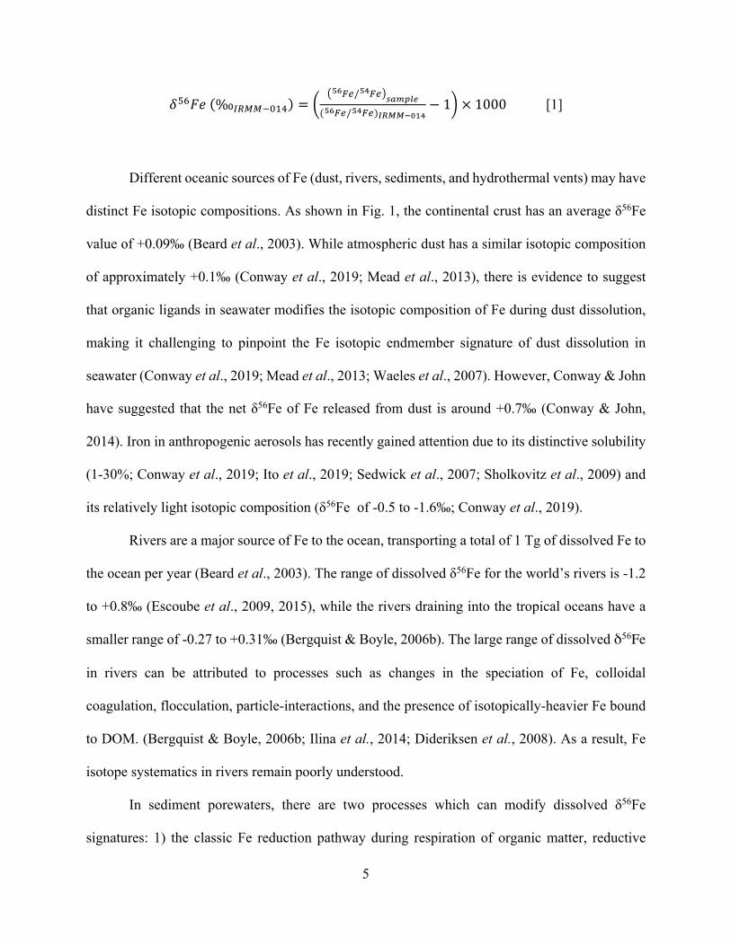
( +,"# / +,"$ )+,--./0$− 1, × 1000 [1]

Different oceanic sources of Fe (dust, rivers, sediments, and hydrothermal vents) may have

distinct Fe isotopic compositions. As shown in Fig. 1, the continental crust has an average δ56Fe

value of +0.09‰ (Beard et al., 2003). While atmospheric dust has a similar isotopic composition

of approximately +0.1‰ (Conway et al., 2019; Mead et al., 2013), there is evidence to suggest

that organic ligands in seawater modifies the isotopic composition of Fe during dust dissolution,

making it challenging to pinpoint the Fe isotopic endmember signature of dust dissolution in

seawater (Conway et al., 2019; Mead et al., 2013; Waeles et al., 2007). However, Conway & John

have suggested that the net δ56Fe of Fe released from dust is around +0.7‰ (Conway & John,

2014). Iron in anthropogenic aerosols has recently gained attention due to its distinctive solubility

(1-30%; Conway et al., 2019; Ito et al., 2019; Sedwick et al., 2007; Sholkovitz et al., 2009) and

its relatively light isotopic composition (δ56Fe of -0.5 to -1.6‰; Conway et al., 2019).

Rivers are a major source of Fe to the ocean, transporting a total of 1 Tg of dissolved Fe to

the ocean per year (Beard et al., 2003). The range of dissolved δ56Fe for the world’s rivers is -1.2

to +0.8‰ (Escoube et al., 2009, 2015), while the rivers draining into the tropical oceans have a

smaller range of -0.27 to +0.31‰ (Bergquist & Boyle, 2006b). The large range of dissolved δ56Fe

in rivers can be attributed to processes such as changes in the speciation of Fe, colloidal

coagulation, flocculation, particle-interactions, and the presence of isotopically-heavier Fe bound

to DOM. (Bergquist & Boyle, 2006b; Ilina et al., 2014; Dideriksen et al., 2008). As a result, Fe

isotope systematics in rivers remain poorly understood.

In sediment porewaters, there are two processes which can modify dissolved δ56Fe

signatures: 1) the classic Fe reduction pathway during respiration of organic matter, reductive

6

dissolution (RD) (Froelich et al., 1979), and 2) release of Fe through ‘non-reductive dissolution’

(NRD) (Homoky et al., 2009, 2013; Radic et al., 2011; Severmann et al., 2006). In the first case,

Fe(III) is reduced to Fe(II) by bacteria in anoxic sediments to produce dissolved Fe(II) that is

lighter than the bulk sediment (-4 to -1.83‰; Homoky et al., 2009, 2013; Severmann et al., 2006).

This process creates isotopically light dissolved Fe2+ in porewaters. In anoxic basins, isotopically

light Fe diffusing out of sediment porewaters can be traced throughout the water column. For

example, dissolved Fe isotope signatures in waters overlying the silled anoxic Santa Barbara Basin

off the coast of California reach values as light as -3.5‰ (John et al., 2012; Severmann et al.,

2010). In contrast, the non-reductive mechanism for sedimentary Fe release is observed to

dominate in oxidizing environments (Radic et al., 2011; Homoky et al., 2013). While this NRD

mechanism is not yet entirely understood, it has been suggested that non-reductive dissolution of

Fe-bearing lithogenic minerals within porewaters occurs without Fe isotope fractionation.

Porewaters in oxidizing environments with dissolved δ56Fe signatures of ~+0.1‰ provide

evidence for this hypothesis (Homoky et al., 2009, 2013). More recently, release of Fe from non-

reductive dissolution of sediment Fe has been proposed to be an important contributor to global

dissolved Fe cycling (Radic et al., 2011; Homoky et al., 2013; Conway & John, 2014).

1.4 Sediment Iron Isotope Cycling Questions

As Fe released via both reductive and non-reductive dissolution is important to the global

marine dissolved Fe cycle, it is essential to understand a) the δ56Fe signatures of both endmembers,

b) whether their signatures fractionate across the sediment water interface, and c) how far the Fe

released is transported through the water column. Past studies have primarily focused on the impact

of either RD or NRD on local and regional Fe cycling, but the distance sediment-derived Fe travels,

7

the speciation of the Fe, and the implications for the global dissolved Fe inventory are much less

clear. To address some of these questions, Fe isotopes have recently been included in modeling

studies to help explain the cycling and distribution of Fe globally (e.g. Koenig et al., 2020).

However, uncertainty and regional differences in potential sedimentary δ56Fe endmembers have

complicated modeling efforts, demonstrating the urgent need for more sampling. Furthermore,

tracing Fe in the ocean released from sediments is complicated by potential isotope fractionation

during re-precipitation, horizontal advection of other water masses, and input from other Fe

sources.

For example, while the δ56Fe endmember for non-reductive dissolution is well defined,

great uncertainty lies with the reductive dissolution endmember, which spans a large range in δ56Fe

within sediment porewaters (-4 to -1.83‰; Homoky et al., 2009; John et al., 2012; Klar et al.,

2017b; Severmann et al., 2006, 2010). The δ56Fe of overlying waters where Fe is attributed to

reductive dissolution ranges from -3.3 to -0.3‰, changing with location and oxygen distributions

(Chever et al., 2015; Conway & John, 2014, 2015; Fitzsimmons et al., 2016; John et al., 2018,

2012; Klar et al., 2018). It remains unclear whether such variability is caused by the primary

isotope signature attributed to RD, fractionation across the interface, or mixing of Fe sources

within the water column. In contrast, while the isotopic signature of Fe from non-reductive

dissolution is thought to be well constrained (Homoky et al., 2013), questions remain about Fe

speciation and the mechanisms of dissolution.

Porewater δ56Fe measurements are also limited to only a few locations around the world,

and mostly on continental margins under highly productive surface waters, where reductive

dissolution is likely to dominate due to high organic carbon fluxes (Homoky et al., 2016). The

restricted global coverage in porewater δ56Fe sampling severely limits our understanding of the

8

isotope signature and form of the Fe which is released into the water column from sediments.

Additionally, while Fe transport away from sediments has been shown in previous studies, the

local physical oceanographic dynamics and bottom water conditions play a large part in

determining the regional fate of Fe away from sediment sources. Furthermore, water-column δ56Fe

data showing the clear influence of sediment processes are also globally sparse, again biased by

being mostly restricted to margins where RD dominates (John et al., 2012; 2018; Conway & John,

2014; Klar et al., 2017b).

Previous studies have spatially separated RD and NRD Fe release based on oxygen and

organic matter flux distributions (Conway & John, 2014; Homoky et al. 2016). This approach

provides an incomplete picture if both sediment dissolution mechanisms occur in the same

sediments. A possible example of such complexity is on the low-oxygen Peru margin, where

release is assumed to be dominated by RD yet water column dissolved Fe isotopic signatures range

from -1.3 to +0.2‰ (Chever et al., 2015; Fitzsimmons et al., 2016; John et al., 2018). Similarly,

in the Eastern North Atlantic Mauritanian oxygen minimum zone, dissolved Fe signatures

attributed to RD only reach -0.5‰ within the benthic nepheloid layer. This relatively heavy δ56Fe

signature has been interpreted as a mixing of sedimentary RD release of Fe with waters above

which have heavy δ56Fe values (+0.3 to +0.7‰; Conway & John, 2014; Klar et al., 2018), but

could also indicate the presence of NRD Fe release.

The three broad questions this thesis will focus on are 1) what is the !56Fe signature coming

from shelf and slope sediments of the South American margin?; 2) is sediment-sourced Fe

transported through surface waters of the South Atlantic?; and 3) is there any evidence of

biological uptake affecting surface δ56Fe signatures in the South Atlantic Ocean?

9

1.5 Research Overview

This thesis addresses some of the uncertainties of sedimentary Fe isotope cycling, using

the South Atlantic Ocean as a case study. Specifically, it presents a detailed focus on regional Fe

cycling near continental margins in the South Atlantic Ocean using dissolved Fe and δ56Fe from

seawater samples collected on the GEOTRACES GA10W (UK) transect (2011) (Fig. 2). Salinity,

temperature, and oxygen concentrations were measured and provide context for water mass

structure (Fig. 3; Schlitzer et al., 2018). Fe and δ56Fe data for this cruise were also measured at

several water-column stations (Fig. 4; Conway et al. in prep; Schlitzer et al., 2018). However, that

study used only 1 L samples and was unable to provide surface δ56Fe data due to low Fe

concentrations. Here, this thesis presents data from two water column stations on the South

American margin and from 2-4 L surface ‘towed-fish’ samples along the whole GA10W section.

This study thus adds to the regional and global picture by providing new constraints on

sedimentary Fe cycling near sediments in the South Atlantic, but is also the first to provide insight

into a region where both reductive and non-reductive dissolution appear to occur simultaneously.

Specifically, data from shelf and slope stations are used to investigate the local isotopic signature

of sediment-derived Fe at the western margin of the South Atlantic, incorporating comparison to

measured porewater depth profiles of dissolved δ56Fe from sediment cores collected on GA10W

(Homoky et al., in prep). These endmembers, the GA10W surface ‘towed fish’ dissolved Fe and

δ56Fe data, and comparison to previous GA10 data, are all used to investigate whether this local

sediment-derived Fe may be traced into the open oxygenated water column and through the surface

waters of the South Atlantic.

Additionally, South Atlantic surface samples provide an excellent opportunity to look more

closely at possible fractionation during biological uptake under Fe-stress, which is difficult to

10

examine in other low-Fe areas and could not be addressed using the lower-resolution, smaller

volume samples that were previously analyzed for the GA10 section (Fig 4; Conway et al., in

prep.). However, the hydrography of South Atlantic and larger volume GA10W surface samples

available for this study are ideal for this purpose. This is because the South Sub-Tropical

Convergence (SSTC), the front where the Antarctic Circumpolar Current (ACC) meets the

subtropical gyre in the South Atlantic, divides GA10W surface samples into distinct groups:

samples within the gyre and samples within the Southern Ocean, south of the SSTC. The eastern

group of samples, which represent Southern Ocean waters, have been identified as from Fe-

stressed waters (Browning et al., 2014). Here, these data are compared with the open oligotrophic

South Atlantic gyre samples to better understand the effect of biological processes on surface

dissolved Fe signatures in this region. This allows insight into whether surface δ56Fe is useful for

tracing Fe sources globally, or may instead be dominantly overprinted by surface biological

processes.

1.6 South Atlantic Oceanographic Setting and Regional Fe Cycling

The South Atlantic Ocean and the sampling locations for GA10W samples in this study are

shown in Fig. 2. Figs 2 and 3 also show the physical oceanography and water mass structure along

the section, modified from Wyatt et al. (2014). The water column in this region is mostly defined

by horizontal water mass flow. Four of the water masses that constitute the water column of

GA10W shown in Fig. 3 originate in high latitude regions of the Northern and Southern

Hemispheres and have distinct salinities and temperatures (Wyatt et al., 2014): Antarctic

Intermediate Water (AAIW) between 500 and 1250 m, Upper Circumpolar Deep Water (UCDW)

between 1250 and 1750 m, North Atlantic Deep Water (NADW) between 2000 and 4000 m, and

11

Antarctic Bottom Water (AABW) as the abyssal layer (>4000 m). In the surface waters (Fig. 2),

warm and salty Sub-Tropical Surface Water (STSW) meets cold and fresh Sub-Antarctic Surface

Water (SASW). This boundary, known as the South Sub-Tropical Convergence (SSTC), defines

the northernmost boundary of the Southern Ocean.

Along the South American margin, the Brazil Current and Malvinas Current combine and

feed into the Argentine Basin, mixing with subtropical South Atlantic gyre waters. The Brazil

Current is defined by its extremely warm (18-28°C) potential temperatures and salinity (35-37)

(Fig. 3; Wyatt et al., 2014). The Malvinas Current is defined by cold temperatures (6°C; Brandini

et al., 2000). The area where these two currents meet, called the Brazil-Malvinas Confluence

(BMC), occurs just east of the Río de la Plata (Boebel et al., 1999; Saraceno et al., 2004). Warm

core eddies often form in the BMC and travel south into the Antarctic Circumpolar Current (ACC)

(Gordon, 1989). High concentrations of macronutrients (silicate and nitrate) and lower salinity are

found in the Río de la Plata estuary (Wyatt et al., 2014). The GA10W surface water transect transits

the confluence zone and the Río de la Plata estuary. The Brazil Current has been shown to transport

Zn (and potentially other trace elements) into the open ocean as it flows away from the South

American margin (Wyatt et al., 2014). By contrast, in the eastern South Atlantic, the marginal

Benguela Current flows toward the African coast, potentially limiting the influence of sediments

on trace metal supply to the GA10W section (Fig. 2). The Agulhas Current, however, has been

shown to transport an Indian Ocean Pb isotope signature, and dissolved Fe into the South Atlantic

via Agulhas rings (Conway et al., 2016; Lutjeharms & Van Ballegooyen, 1988; Paul et al., 2015b;

Schlosser et al., 2019), suggesting that episodic transport of Fe and other trace elements may

influence surface ocean concentrations (Conway et al., 2016; 2018).

12

Along the GA10W section, dissolved Zn concentrations show the dominance of Southern

Ocean water masses (Wyatt et al., 2014), whilst dissolved Fe distributions in Fig 4. more strongly

point to Fe sources at the margins (Schlitzer et al., 2018; Conway et al., in prep). Dissolved Fe

concentrations are less than 1 nmol kg-1 in the deep ocean and less than 0.1 nmol kg-1 above 500

meters (Schlitzer et al., 2018; Conway et al., in prep). Near the margins and mid-ocean ridge,

however, dissolved Fe concentrations can reach 2 nmol kg-1 (Schlitzer et al., 2018; Conway et al.,

in prep). Although dust transport from Patagonia provides higher dust loads to the western South

Atlantic, this occurs mostly south of the GA10W section (Johnson et al., 2011). Biological uptake

in the surface ocean as well as low dust supply to this region (Chance et al., 2015; Mahowald et

al., 2005) likely account for much of the low surface Fe concentrations, whereas fluvial and

sedimentary influences could explain the higher concentrations near the margins (Conway et al.,

in prep).

In contrast to dissolved Fe concentrations, dissolved δ56Fe values through the GA10W

transect reflect water masses of the South Atlantic (Fig. 4; Conway et al., in prep). AAIW, UCDW,

and NADW/AABW show Fe isotope signatures of -0.2, -0.1, and +0.25‰, respectively (Conway

et al., 2016). Although available Fe isotope data from the surface ocean across the GA10W section

cluster within the range of crustal values (+0.1‰), this may well be an artifact of scarce surface

data and poor analytical precision at such low Fe concentrations (<0.1 nmol kg-1). As such, Fe

isotope cycling in surface waters of the South Atlantic remains poorly constrained (Conway et al.,

in prep). However, in surface waters and at depth closer to the South American margin, there is

preliminary evidence to suggest a sedimentary input of Fe from the margin (Conway et al., in

prep). This thesis uses a higher-resolution, larger-volume surface sample set, as well as shelf and

slope stations, to investigate this in more detail.

13

Figure 1. The Fe isotope signatures of oceanic dissolved Fe sources (modified from Tim

Conway, unpublished).

14

Figure 2. Map of the study site in the South Atlantic Ocean. GA10W fish samples shown in white, and depth profiles shown in green. AC: Agulhas Current, BC: Brazil Current, MC: Malvinas Current, RP: Río de la Plata, RPP: Río de la Plata, SASW: Sub-Antarctic Surface Water, SSTC: South Sub-Tropical Convergence, STSW: Sub-Tropical Surface Water (modified from Wyatt et al., 2014).

15

Figure 3. Distributions of potential temperature, salinity, and oxygen concentrations along GA10W. Section plots are reproduced from the GEOTRACES e-atlas (http://www.egeotraces.org; Schlitzer et al., 2018). Water masses are defined following Wyatt et al. (2014): AABW: Antarctic Bottom Water, AAIW: Antarctic Intermediate Water, AC: Agulhas Current, BrC: Brazil Current, NADW: North American Deep Water, SASW: Sub-Antarctic Surface Water, STSW: Sub-Tropical Surface Water, UCDW: Upper Circumpolar Deep Water.

16

Figure 4. Distributions of dissolved Fe concentrations and δ56Fe along GA10W. Section plots are reproduced from the GEOTRACES e-atlas (http://www.egeotraces.org; Schlitzer et al., 2018). Water masses follow Fig. 3: AABW: Antarctic Bottom Water, AAIW: Antarctic Intermediate Water, NADW: North American Deep Water, UCDW: Upper Circumpolar Deep Water.

17

CHAPTER II

METHODS

2.1 Sample Collection

Seawater samples were collected using trace-metal clean techniques during the UK

GEOTRACES 40°S GA10W transect (JC068) aboard the R.R.S. James Cook in December 24,

2011 to January 27, 2012 (Fig. 2; Cutter & Bruland 2012; Conway et al., 2016; Wyatt et al., 2014).

Water column samples were collected using a titanium CTD package with twenty-four 10 L

Teflon-coated bottles and deployed using a plasma polyethylene rope. The bottles were transferred

to a container fitted as an ISO Class 5 trace-metal clean laboratory on board. One hundred and

twenty-three 1-liter surface seawater samples were collected from a towed ‘fish’ alongside the ship

(2-3 m depth) by pumping seawater into a trace-metal clean lab to be filtered. Surface fish samples

were collected approximately every 2-4 hours in between oceanographic depth stations. All

seawater samples were filtered using a 0.2 µm AcropakTM Supor polyethersulfone membrane filter

capsule. Pressure was applied to bottles to speed up sampling of water column samples. Samples

were acidified back on shore to pH ~2 by addition of conc. Ultrapure HNO3 and stored until

processing (Klar, pers. comm.).

2.2 Clean Laboratory Procedures

All clean work was carried out under ISO Class 5 laminar flow air within an ISO Class 6

trace-metal clean lab at the University of South Florida College of Marine Science. Dupont Tyvek

18

high-density polyethylene (HDPE) suits and rubber clogs were worn in the lab to limit

contamination and HDPE sleeves were worn when working in a clean bench to further limit trace-

metal contamination. Vinyl gloves were worn to protect from acid contact, while polyethylene

(PE) gloves were worn over the vinyl gloves and were used for all handling of samples and

materials to reduce trace-metal contamination. All water used was ultrapure (18.2 MΩ) from a

Thermo Scientific Barnstead GenPure Ultrapure water (UPW) system. Trace-metal grade Fisher

Scientific hydrochloric (HCl) and nitric (HNO3) acids were cleaned using a Savillex

perfluoroalkoxy alkane (PFA) acid purification system to produce clean concentrated acids.

Hydrogen peroxide (H2O2) used was Optima grade from Fisher Scientific. All plasticware used

was cleaned following standard procedures at USF (Conway et al., 2013). Low-density

polyethylene (LDPE) bottles were cleaned by submerging in a weak detergent, and then

submerging in a 1 M HCl acid bath for approximately seven days, with extensive rinsing with

UPW after each step. New Savillex perfluoroalkoxy alkane (PFA) vials, fluorinated ethylene

propylene (FEP) bottles, and polytetrafluoroethylene (PTFE) columns were cleaned by sequential

soaking in 7 M HNO3, 6 M HCl, 2% HNO3 and 3 M HNO3 on a hotplate set to 150°C for two days

each, rinsing with UPW after each step. Between samples, PFA vials were cleaned with 3 M HNO3

on a 150°C hotplate overnight.

2.3 Chemical Methods

Extraction and purification methods for Fe in seawater follow previously published

methods (Conway et al., 2013; Sieber et al., 2019). These are described in more detail below.

19

2.3.1 Extraction from Seawater Matrix

Based on dissolved Fe concentrations previously measured by collaborators, an Fe double-

spike was added to each seawater sample to attain an optimal sample to spike ratio of 1:2. 1 mL

of 10 mmol L-1 H2O2 per liter was also added to each sample to oxidize all the dissolved Fe in the

sample to Fe(III). At least 24 hours later (to allow the double spike to equilibrate), ~1.5 g (2.75

mL) of Nobias PA-1 resin beads (Hitachi High Technologies) was added to each sample. Samples

were then shaken for at least 2 hours using an orbital shaker table. Resin beads (with Fe bound to

functional groups) were then filtered out of the sample using a PFA filter rig and Whatman®

NucleporeTM (8 µm pore size) polycarbonate filter membrane under vacuum, following Conway

et al. (2013). Briefly, each sample was poured into the filter rig, allowing for all liquid to flow

through the filter, with resin beads (50 µm size) collected onto the membrane. One volume of the

filter reservoir (~150-200 mL) of ultrapure water (UPW) was then poured through to rinse off any

salt. Metals were then eluted into a 30 mL Savillex vial in 6 aliquots of 5 mL 3M HNO3. Samples

were then evaporated to dryness on a hotplate overnight at 180°C. The resin was rinsed with 150

mL of 2% HNO3, ~30 mL 3M HNO3, and 2x100 mL UPW between samples, and stored in 3M

HNO3 between use.

2.3.2 Trace Metal Purification

Evaporated samples were re-dissolved in 180 µL concentrated HNO3 plus 20 µL

concentrated H2O2. Samples were capped and put on a hotplate at 180°C to reflux for about 1-2

hours in order to oxidize any organic residue. Samples were then evaporated to dryness, before

being re-dissolved in 200 µL 7M HCl with 0.001% H2O2 (made by adding 50 µL concentrated

H2O2 to 500 mL of 7M HCl) to prepare samples for column chemistry. Approximately 20 µL pre-

20

cleaned Biorad AG-MP1 anion-exchange resin was added to each cleaned PTFE micro-column.

Four aliquots of 200 µL 7M HCl with 0.001% H2O2 were added to clean each column. Then, five

aliquots of 60 µL UPW were added rinse metals off the resin. To condition the resin functional

groups before sample introduction, 200 µL 7M HCl with 0.001% H2O2 was added. Samples (in

200 µL of 7M HCl with 0.001% H2O2) were then added to the columns and allowed to drip

completely through, binding Fe(III) in chloride form to the resin while the liquid is discarded.

Then, 14 aliquots of 30 µL 7M HCl with 0.001% H2O2 were added and the eluted salts were

discarded. Following this, Fe was eluted using 12 aliquots of 30 µL 1M HCl and collected in a 7

mL Savillex PFA vial. Samples were then evaporated to dryness on a hotplate at 180°C for

approximately one hour. Samples were redissolved with 0.6 mL 2% HNO3 v/v for MC-ICP-MS

analysis.

2.4 Analytical Methods

Samples were analyzed for Fe isotope ratios using a Thermo Neptune Plus MC-ICPMS in

the MARMITE labs at the Tampa Bay Plasma Core Facility at USF’s College of Marine Science.

Samples, dissolved in 2% HNO3 v/v, were introduced to the plasma via a PFA nebulizer into an

ESI Apex Ω desolvator. A nickel Jet ‘sampler’ cone and an aluminum ‘X type’ cone were used to

boost Fe sensitivity. A drawback of using ICPMS for Fe is that Argon is used as the plasma gas,

and argide interferences are generated at all four stable Fe masses (for example, 54Fe: 40Ar14N,

56Fe: 40Ar16O, 57Fe: 40Ar17O+, 58Fe: 40Ar18O+). Partial resolution of Fe from ArO or ArN was

achieved by using a ‘high’ resolution slit and mode (resolving power >8000). Typically, resolving

power was >9000. The Apex Ω was chosen over a regular spray chamber or an Apex Q desolvator

because it dramatically boosts Fe sensitivity while reducing polyatomic interference formation

21

(ArO, ArN). The measurement mass position for Fe was chosen as the center of the Fe shoulder.

This position was determined manually by averaging the masses of the left edge of the Fe shoulder

and the start of the ArO+Fe shoulder. Six isotopes were measured during analysis: 52Cr, 54Fe, 56Fe,

57Fe, 58Fe, and 60Ni. 52Cr and 60Ni voltages were measured to correct for isobaric interferences of

54Cr on 54Fe and 58Ni on 58Fe, using a mass-bias corrected abundance ratio based on 56Fe/57Fe. To

account for instrumental background, an on-peak blank correction was used to measure the

intensities of Fe in 2% HNO3 before each sample was measured. Assuming a take up time of

approximately one minute, a typical analysis of one sample consisted of one minute in the wash,

two short analyses of blank 2% HNO3 (wash and pre-wash), a full analysis of an on-peak blank

2% HNO3, and a full analysis of a sample. The total duration of analysis for one sample was

approximately 11 minutes.

Instrumental mass bias on Fe during analysis was corrected using the double spike

technique. Double spike was added to samples before processing at a sample:spike ratio of 1:2, an

optimal ratio which minimizes internal error on the isotope ratios (John, 2012; Lacan et al., 2008).

Because the double spike was added before sample processing, it also allowed for correction of

potential isotope fractionation during chemical processing. Use of an internal double spike is

advantageous over other methods (such as standard-sample bracketing) because it allows

determination of mass bias during sample measurement (John, 2012), and thus accounts for any

rapid changes in mass bias. The double spike composition was previously established at ETH

Zürich (ETHZ), and it has been established that this calibration holds at USF. Isotope ratios were

corrected for mass bias following a standard double spike data reduction scheme in Microsoft

Excel (Conway et al., 2013; Siebert et al., 2001). To confirm the spike calibration was appropriate

in each session, mixtures of standard and spike with varying ratios between 1:5 and 5:1, and

22

various concentrations of the optimal 1:2 ratio were analyzed before each analytical session.

Spiked samples were measured in groups of five, bracketed by two mixtures of the zero standard

(IRMM-014) with the double spike (100:200 ng/g sample:spike), to account for any instrumental

drift. Based on previous work (Sieber et al., in review), and the concentration standards run

alongside these samples, δ56Fe data are accurate when the sample voltage is greater or equivalent

to that of a 10 ng g-1 standard, which typically corresponds to a seawater sample of 90 pmol kg-1

in 1 L (25 pmol kg-1 in 4 L). Data is not reported below this voltage. Fe isotope ratios (δ56Fe) of

samples are always expressed relative to the average of the respective two bracketing standard-DS

mixtures. A secondary standard (NIST-3126a) was measured with each group of samples to check

accuracy and monitor long term analytical precision.

One of the other advantages of using a double spike for instrumental mass bias correction

is that it also allowed determination of Fe concentration. Addition of a known amount of double

spike prior to processing allowed for precise and accurate determination of Fe concentrations using

the isotope dilution technique. Briefly, double spike (with a known amount of Fe and known

isotopic composition) was added to each sample before processing. The spike concentration was

determined using gravimetric standards made from Fe metal (Sieber et al., in review). Accurate,

blank-corrected 57Fe and 56Fe voltages were a byproduct of isotope analysis for each sample.

Because the composition of the double spike as well as the amount of spike added to each sample

is known, the Fe concentration in samples can be calculated using the composition of Fe and the

mass of the seawater sample.

23

CHAPTER III

RESULTS AND DISCUSSION

3.1 Procedural Blanks

Procedural blanks were processed to ensure cleanliness and reproducibility. Ten 100 mL

UPW samples were acidified, processed, and analyzed for Fe concentrations using the same

chemical and analytical method as seawater samples. The mean Fe amount of the blanks was

0.24±0.04 ng of Fe (n=10), better than or equivalent to that shown previously for this method

(Conway et al., 2013).

3.2 Precision and Accuracy

Since it is not typically possible to do multiple replicate analyses of seawater samples for

δ56Fe due to volume requirements, Sieber et al. (in review) was followed and analytical external

precision of δ56Fe measurements was estimated using a NIST-3126a Fe reference solution with a

concentration of 100 ng g-1 (equivalent to a 1 nmol kg-1 sample) and the optimal spike sample ratio

of 1:2. As shown in Fig. 5, the NIST-3126a solution has been measured 190 times over 15

analytical runs over three years at USF, with a mean δ56Fe of +0.36 and a 2SD of 0.04‰.

Additionally, in collaboration with Elemental Scientific Inc. the USF methods were used to

conduct full procedural replicate analyses (n=5) of a GA02 Atlantic Ocean seawater sample for

comparison with a new automated Fe isotope method. The Fe concentrations and isotope

signatures of the five replicates had a 2SD of 0.03 nmol kg-1 (2%) and 0.04‰, respectively,

24

identical to the long term NIST precision. Previous work in Conway et al., 2013 showed that an

uncertainty of 0.05‰ was appropriate over a range of 0.1-1.8 nmol kg-1 for Southern Atlantic

seawater, similar to the 0.04‰ for the NIST standard at USF (Conway et al., 2016). A precision

of 0.04‰ is smaller than or equivalent to most standard internal errors of analysis in this dataset

(2SE 0.02 to 0.29‰). The 2SD of the NIST solution (0.04‰) is therefore considered a

representative estimate of uncertainty on δ56Fe measurements for most samples. When the standard

internal error (2SE) of an individual sample is larger than 0.04‰, the 2SE is considered a more

conservative estimate of uncertainty instead. The accuracy of the analytical procedure was also

assessed by comparing the measured mean δ56Fe of the NIST-3126a to previous measurements by

Rouxel and Auro (+0.39±0.13‰) and Conway et al., 2013 (+0.32±0.02‰). For Fe concentrations,

the accuracy of this method has been demonstrated previously (Conway et al., 2013; 2016), and

for precision, a 2% error was shown by Conway et al. (2013), which was the same as measured on

the procedural replicate samples.

3.3 GA10W Results

Here, dissolved Fe and δ56Fe data are presented for 65 GA10W samples (Fig. 2) include

18 water column samples from Stations 22 and 24 (Figs 6, 7), and 47 surface ‘fish’ samples (Fig.

8 and Table 1). With a water depth of 60 meters, Station 24 is defined as a shelf station. Station

22, with a depth of 1500 meters, is defined as a slope station. The surface fish samples from these

two stations are consistent with the lower-salinity influence of the Río de la Plata plume and are

discussed together with the other surface samples separately in Section 3.3.2 GA10W Surface

Transect.

25

3.3.1 GA10W Margin Stations 22 and 24

The entire water column at shelf Station 24 (Fig. 7) is generally high in dissolved Fe (>1.0

nmol kg-1), with the highest concentration (2.5 nmol kg-1) at a depth of 50 m, 10 m above the

sediment-water interface. Dissolved oxygen concentrations are consistent at 215 µmol kg-1 from

the surface down to 30 m, below which they decline to 195 µmol kg-1. This small decline in

dissolved oxygen concentration is accompanied by an increase in dissolved Fe concentration at

depth. Dissolved δ56Fe values at Station 24 generally show relatively homogenous values

throughout the profile (Fig. 7), with a mean isotope signature of -0.17±0.03‰, perhaps indicative

of a similar Fe source throughout the profile. Overprinted on this background, there is a δ56Fe

excursion to -0.80±0.03‰ at 23 m, which corresponds with a minor elevation in Fe concentration

(1.27 nmol kg-1).

At Station 22, dissolved Fe shows distinctly elevated concentrations of 2 nmol kg-1 in the

water column at a shallow (~100 m) and a deep (~1250 m) horizon compared to the rest of the

profile (0.5-0.6 nmol kg-1; Figs. 6, 7). This shallow maximum in Fe concentration has a mean δ56Fe

signature of -0.28±0.03‰ (1SD), while the deep Fe concentration maximum has a mean δ56Fe

signature of -0.66±0.03‰ (1SD). Both the shallow and deep Fe concentration excursions

correspond to relatively low dissolved oxygen (175-180 µmol kg-1). These high Fe concentrations

linked to light δ56Fe throughout the water column at shelf Station 24 and at two distinct horizons

at slope Station 22 likely point to local sedimentary addition of Fe on the shelf/slope. It is also

worth noting that δ56Fe values are also lighter than 0‰ within the whole horizon at Station 22

associated with AAIW (Fig. 6; 600-1600 m; S <34.4), and then transition to isotopically heavier

values (>+0.2‰) within NADW, as observed in previous studies (Abadie et al., 2017, Conway et

al. 2016, Lacan et al., 2008).

26

3.3.2 GA10W Surface Transect

Here, Fish data are described in sequence, moving from the South American margin, across

the open ocean and approaching the South African shelf (Figs 8, 9). From the South American

margin out to ~35°W, surface dissolved Fe concentrations are elevated (>0.3 nmol kg-1), but show

a great deal of variability (0.2-3.0 nmol kg-1), pointing to the far-reaching and variable influence

of Fe sources on the margin across this whole surface region (Fig. 8). Dissolved δ56Fe values vary

from -1.2 to +0.4‰ across this western region of the based transect. Due to the confluence of water

masses and riverine discharge from the Río de la Plata (Fig. 2 and 4), however, this region can be

grouped into four different sections based on measured physical and chemical properties from

surface samples (see Fig. 9).

Nearest the coast, samples with a salinity of ~32, temperature of 21.5-23.5°C, and

fluorescence of 3.6-4 μg L-1 are here considered coastal waters (CW). Moving seaward, farther

east, salinity declines, reaching a minimum of <29 within lower-salinity water from the Río de la

Plata Plume (RPP; Figs 6, 9; Schlosser et al., 2019) while silicate concentrations are elevated (21

µM). Fluorescence, a proxy for biomass, declines to less than 3.6 μg L-1 within this interval. The

core of the RPP influence is shown as a darker blue in Fig. 9. Extending outside this region, the

lesser influence of the RPP is shown as the light blue bands in Fig. 9, as the lower-salinity water

mixes with surrounding waters. Moving eastward, a substantial rise in salinity to 36 and a slight

increase in temperature point to the influence of the southward-moving Brazil Current (Wyatt et

al., 2014). The influence of the Brazil Current can be seen in salinity as far as ~50°W. However,

within the Brazil Current, a sharp drop in salinity to 34 is seen at 53-52°W, along with a slight

decrease in temperature to 24°C. This most likely corresponds to a filament or eddy of the

northward-moving Malvinas Current (MC) within the Brazil Current (BC), as is typical of the

27

region of the Brazil-Malvinas Confluence (BMC; Boebel et al., 1999; Saraceno et al., 2004).

Fluorescence shows a maximum at 4.5 μg L-1 within the Malvinas Current, consistent with primary

production fed by nutrients from within the Sub-Antarctic waters of the Malvinas Current.

Dissolved Fe and δ56Fe values show great variability through these regions. The coastal

waters exhibit dissolved Fe concentrations of 0.6-2.0 nmol kg-1 and have δ56Fe values of ~0‰

(Fig. 9). A range of δ56Fe (-1.2 to +0.1‰) is seen within the low-salinity core of the RPP, possibly

indicating a mix of distinct Fe sources, with dissolved Fe at 1 nmol kg-1 (Figs 6, 9). In the regions

where the salinity rises out of the core of the RPP, interpreted as the plume mixing with

surrounding waters, δ56Fe values are isotopically heavy to the west (+0.4‰) and light to the east

(-0.6‰) while dissolved Fe concentrations (0.3-0.6 nmol kg-1) are lower than within the core RPP.

The Brazil Current region then sees dissolved Fe concentrations reach a maximum of 3 nmol kg-

1, while δ56Fe values return to -0.1 to +0.1‰ (Fig. 9). Dissolved Fe concentrations then decline

moving eastward through the hypothesized Malvinas Current eddy, but close to crustal δ56Fe

values (-0.2 to +0.2‰) are still observed.

Moving east, from 40°W to 25°W, very low (<0.1 nmol kg-1) dissolved Fe concentrations

are observed which continue to be linked to crustal δ56Fe signatures, as fluorescence declines to

very low levels, typical of the South Atlantic Gyre (Fig. 8; Browning et al., 2014). Between 20°W

and 10°E, both fluorescence and dissolved Fe concentrations are extremely low (<0.2 µg L-1 and

<0.1 nmol kg-1), however, δ56Fe values increase to +0.5 to +1.0‰ (Fig. 8). This region corresponds

to the cold (<16°C) and nutrient-rich, but low Fe, waters of the Southern Ocean (Figs 8, 10). East

of 10°E (Fig. 9), temperature increases from 14°C to about 20°C, indicating the presence of coastal

waters and possibly the influence of the warm Agulhas Current. However, dissolved Fe

concentrations remain low here (0.1 nmol kg-1), while δ56Fe values fluctuate around a mean of

28

+0.5±0.16‰ (1SD). The samples closest to the African coast show a small but substantial increase

in dissolved Fe concentrations (0.2 nmol kg-1), silicate (6 µM), and fluorescence (0.6 μg L-1), along

with a decrease in temperature to 15°C (Fig. 9). Similar to the South American margin shelf, the

surface fish sample nearest to the African margin has a light Fe isotope signature (-0.47±0.11‰).

3.4 GA10W Discussion

Here, the local isotopic signature of sediment-derived Fe on the South American margin

will be discussed by comparing water column dissolved δ56Fe data to dissolved δ56Fe from

sediment porewaters extracted from cores collected on GA10W (Homoky et al., in prep). This

comparison provides insights into the nature and isotopic signature of the Fe released by sediments

along the shelf and slope of this margin. Using this information, evidence is shown to support that

Fe from sediments is transported away from the margin, both at depth and at the surface. Finally,

δ56Fe data from the open South Atlantic gyre provide insight into Fe isotope fractionation during

biological uptake and surface cycling of dissolved Fe.

3.4.1 Shelf and Slope Sediment Isotope Signature and Influence

δ56Fe results from slope and shelf stations of GA10W, coupled with porewater data, may

allow assignment of a Fe isotope signature to sediment-derived Fe on the shelf and slope of the

South American margin. Assuming that the variability in Fe isotope signatures associated with

elevated Fe concentrations near the sediments comprises a mixture of Fe sourced from reductive

or non-reductive sediment dissolution, a two-component mixing model was used to calculate the

fraction of each source to a water-column sample (Equation 2; Conway & John, 2014).

29

!!""##$%&'( = (!!""#) × (*) + (!!""#) × ()) [2]

To do this calculation, appropriate δ56Fe endmembers for reductive (RD) and non-

reductive dissolution (NRD) were chosen. Because large variability in the δ56Fe RD endmember

can be seen from the literature, the more-relevant local GA10W sediment porewater data were

used to inform mixing calculations. For the RD δ56Fe endmember, the mean δ56Fe signature of the

reductive zone of porewaters measured in sediment cores from GA10W stations 18-24 (-

1.05±0.26‰ 2SD; n=19; Homoky et al., in prep.) was used. Notably, this RD endmember is

significantly heavier than that of δ56Fe signatures in porewaters underlying productive shelf

environments with low bottom water oxygen. For example, the California and Oregon margin and

the Celtic Sea Shelf exhibit extremely light porewater δ56Fe values, down to -3.4‰ (Homoky et

al., 2009, 2013; John et al., 2012; Klar et al., 2017b; Severmann et al., 2006, 2010). Consistent

with these data, previous studies have used a lighter RD endmember value for isotope mixing

calculations (-2.4‰; Conway & John, 2014). However, this study provides a more locally-

informed RD δ56Fe endmember based on a range of shelf, slope and abyssal sediments on the

South American margin. This approach demonstrates the value of combining porewater and water

column sampling for Fe isotopes. This endmember also agrees reasonably (within 2SE) with the

δ56Fe signature of -1.27‰ measured previously within Amazon shelf porewaters (Bergquist &

Boyle, 2006b). For the non-reductive endmember, a crustal value of +0.1‰ was used (Homoky et

al., 2013). The caveats of using this mixing model approach are the assumptions of fixed

endmembers, that reductive and non-reductive sediment dissolution are the only sources of Fe to

these samples, and that the endmember δ56Fe values are not altered across the sediment-water

interface.

30

Using these endmembers, the percentage of Fe released at depths of 50 m at the shelf (at

Station 24) from sediment RD is calculated as 16%, while 84% is from NRD sediment dissolution.

The shallow source of Fe at station 22 shows similar values (reductive: 26%; non-reductive: 74%).

The δ56Fe value of the shallow source of Fe at both Stations 22 and 24 is -0.28±0.03‰ and -

0.17±0.03‰, respectively. This similarity in overall proportions of RD and NRD, as well as δ56Fe

values, likely points to a similar Fe source at both stations. Accordingly, the overall isotopic

signature of the shelf source of Fe in this local region is broadly characterized to be -0.2‰. This

source may be traceable through the surface of the GA10W section (see Section 3.4.2 Fe Sources

in Western Surface Waters and the Influence of the Río de la Plata). By contrast, the deeper

sedimentary source of Fe observed at Station 22 is calculated as 62% RD and 38% NRD. Thus, at

Stations 22 and 24, non-reductive sediment dissolution seems to be the dominant source of Fe near

100 m, while reductive sediment dissolution is more dominant at depth. At first glance, this is

perhaps counterintuitive given that shallow shelf sediments typically have a greater organic carbon

supply compared to deep-water sediments, which should equate to higher Fe fluxes (Elrod et al.,

2004; Homoky et al., 2016). Dissolved oxygen is also similar at both depths (Fig. 6). Thus, a higher

flux of Fe might be expected from within the shallower sediments. However, at Station 24, the

sediments consist of highly permeable sands (Homoky et al., in prep), therefore oxygen can

penetrate deep into the sediments. In contrast, the sediments on the slope at Station 22 are much-

finer grained, limiting the penetration of oxygen deeper into the sediment. Organic carbon flux to

the benthic sediments is also greater at Station 22 than 24 (Homoky et al., in prep). Thus, at Station

22, the greater organic carbon flux and shallower anoxic layer likely provides an environment that

brings lighter δ56Fe closer to the sediment-water interface (Homoky et al., in prep), resulting in a

greater influence of reductive release compared to Station 24. This observation again highlights

31

the utility of coupling local sediment coring and porewater analyses with water column profiles in

basin-scale surveys.

Farther off the shelf, similar to Station 22, Station 21 also shows elevated dissolved Fe

concentrations (2 nmol kg-1) at ~1500 m (Fig. 6; Conway et al., in prep; Schlitzer et al., 2018),

which are also associated with light δ56Fe of ~-0.5‰ (Fig. 6). This similarity between Stations 22

and 21 may suggest that the deep sediment source of Fe at Station 22 is transported at least 75 km

east through the mid-water column to Station 21 through the limited oxygen minimum zone

(OMZ). If so, the slope source endmember in this region can be characterized as a δ56Fe of -

0.66±0.03‰. This observed Fe transport through low-oxygen water is consistent with a range of

recent studies that have shown that dissolved Fe and light δ56Fe persist through OMZs (John et

al., 2012, 2018; Chever et al., 2015; Conway & John, 2015). In contrast, however, the shallow

source of Fe seen at Station 22 does not appear to be transported to Station 21, where surface δ56Fe

values are instead isotopically heavy (Conway et al., in prep). Higher oxygen concentrations and

zonal surface currents may contribute to this loss of Fe source signature. The heavier δ56Fe values

seen in the surface of Station 21 might instead be attributed to dust deposition (Conway & John,

2014).

3.4.2 Fe Sources in Western Surface Waters and the Influence of the Río de la Plata

In the results, four regions of the western portion of the GA10W transect were broadly

defined, Coastal Waters, Río de la Plata Plume Waters, Brazil Current Waters and Malvinas

Current Waters. These different water masses mix within the Brazil-Malvinas Confluence Zone,

potentially leading to a complicated mixing of Fe sources and processes. The samples in the

32

Coastal Waters region have near-crustal δ56Fe values, likely signifying a NRD sediment source,

as has been observed near margins in the North Atlantic (Conway & John, 2014).

Transiting into the influence of the Río de la Plata Plume, the slightly heavier δ56Fe value

of +0.4‰ could be linked to Fe bound to organic molecules from terrestrial material or organic-

rich tropical soils, which are thought to have a heavy Fe isotope signal (Akeman et al., 2014;

Bergquist & Boyle, 2006b; Dideriksen et al., 2008; Ilina et al., 2014). Approaching the core of the

Río de la Plata Plume, where salinity reaches as low as 28, an excursion to significantly light δ56Fe

is seen (-1.21‰). Notably, this is the lightest δ56Fe observed anywhere in the dataset (Table 1).

To the east, as salinity rises slightly, δ56Fe (-0.67‰) remains light. The light δ56Fe excursion

associated with the influence of the RPP is lighter than the limited tropical riverine δ56Fe datasets

(-0.4 to +0.7‰) and most of the data from Arctic river systems (Akerman et al., 2014; Escoube et

al., 2015; Ilina et al., 2013; Ingri et al., 2006; Mulholland et al., 2015; Revels, 2018), but is

consistent with small Arctic rivers (Escoube et al., 2015).

Perhaps the most relevant dissolved Fe isotopic comparisons that exist in the literature for

the Río de la Plata would be the organic-rich ‘blackwater’ Río Negro tributary (+0.2 to +0.6‰)

and the Río Solimões tributary (-0.4 to 0‰) of the Amazon river, together with the downstream

mixing δ56Fe signature of the two tributaries (0 to +0.6‰; Bergquist & Boyle, 2006b; Mulholland

et al., 2015; Revels, 2018). Previous studies have attributed the light values seen in the Solimões

to the potential influence of weathering of rocks or plants (Bergquist & Boyle, 2006a; Mulholland

et al., 2015), while weathering tropical lateritic soils see crustal signatures (Akerman et al., 2014).

Organic-rich soils are thought to result in isotopically heavy Fe (Escoube et al., 2015; Ingri et al.,

2006). Although the Río de la Plata dataset is very limited, our potential riverine δ56Fe signatures

(+0.4 to -1.2‰) include a range of values, with some much lighter than that seen in the Amazon.

33

These lighter signatures could be related to isotopically light primary Fe signatures in the river

from weathering rocks or plants (Bergquist & Boyle, 2006b), or Fe(II) released by both NRD and

RD from margin or river sediments, while heavy signatures likely relate to organic-bound Fe

(Bergquist & Boyle, 2006a; Ilina et al., 2013).

However, it is also important to consider that our samples have a salinity >28, which is

consistent with a plume that has already undergone estuarine mixing. Studies have shown that

flocculation removes greater than 75% of riverine Fe upon mixing with seawater, while mixing

experiment results predict that flocculation causes Fe isotope fractionation, driving remnant

dissolved δ56Fe to light values of -1 to -2‰ (Bergquist & Boyle, 2006b; Sholkovitz, 1976;

Sholkovitz et al., 1978). This could provide an alternate explanation for the very light Fe seen in

our samples, but would require more systematic sampling to test. Overall, even though salinity in

this ‘plume’ is high, our data provide evidence that riverine and estuarine processes play a major

role in the fate of Fe and δ56Fe being transported from rivers into the open ocean. This study

highlights the need for more river-to-ocean Fe isotope studies.

The next region shows the influence of the Brazil and Malvinas Currents (Fig. 9). δ56Fe

values are close to crustal in these waters, indicative of a sediment supply of Fe from the margin.

Moving farther east, dissolved Fe concentrations decrease and δ56Fe continue to show crustal

values (~+0.1‰). The sediment source endmember that was identified for the shelf (Section 3.4.1

Shelf and Slope Sediment Isotope Signatures and Influence), with a δ56Fe signature of -0.2‰,

agrees relatively well with these crustal surface δ56Fe values, indicative of the lateral transport of

sediment Fe hundreds of kilometers away, as seen in previous studies (Conway & John, 2014).

However, the slightly heavier values in the surface of the open gyre region may suggest that the

NRD source from the shelf persists, while the RD source is lost via precipitation during transport.

34

If so, the NRD-sourced Fe has a longer residence time, which may be because the Fe is present in

the colloidal phase rather than as truly-dissolved Fe (Homoky et al., 2009, in prep). This behavior

would be consistent with observations of long-distance transport of NRD Fe in the western North

Atlantic (Conway & John, 2014). By tracing the NRD source of Fe through surface waters, this

thesis suggests that shelf sediments provide a consistent Fe supply to the surface of the western

South Atlantic gyre.

3.4.3 Biological Cycling of Fe Isotopes South of the SSTC

Onboard incubation experiments used the change in photochemical efficiency (Fv/Fm) to

highlight a portion of the GA10W section which is Fe-stressed (shown in Fig. 10; Browning et al.,

2014). These Fe-stressed waters correspond with Southern Ocean waters south of the SSTC (Fig.

10). These waters contain extremely low dissolved Fe concentrations (<0.1 nmol kg-1) and high

nitrate concentrations, consistent with Southern Ocean Fe-limited HNLC waters (Boyd &

Ellwood, 2010; de Baar & de Jong, 2001; Schlitzer et al., 2018). Deep waters are upwelled in these

regions to provide an abundance of major nutrients, but do not provide sufficient dissolved Fe for

full utilization (Boyd & Ellwood, 2010). Here, the extremely low dissolved Fe concentrations

suggest that biological uptake of Fe is influential, providing an opportunity to investigate the

influence of biological uptake on dissolved δ56Fe in a region with little surface dust addition. The

sudden transition to the Fe-stressed Southern Ocean waters at 20°W corresponds with a distinct

transition from crustal to heavy δ56Fe compositions (mean of +0.69±0.17‰; n=7). These heavy

δ56Fe values in the Fe-limited region are consistent with several recent studies from the open

Southern Ocean and from within isolated eddies and polynyas in the Southern Ocean (Ellwood et

al., 2015; 2020; Sieber et al., in review). Those studies identified the interplay of Fe binding to

35

organic ligands, biological uptake, and sinking particulate regeneration, in driving surface Fe

isotope cycling under Fe-limited regimes (Ellwood et al., 2015, 2020; Sieber et al., submitted).

The effect of these processes are also likely to explain the heavy δ56Fe values along GA10W.

3.4.4 Sediment Supply from the African Margin

With elevated silicate, and a slightly elevated dissolved Fe concentration, surface samples

near the African margin display a dissolved δ56Fe signature of -0.47±0.11‰ (Fig. 9). This is

consistent with previous nearby observations: the δ56Fe depth profile near this location at Station

8 of GA10 (D357 cruise 2010) shows water column dissolved δ56Fe reaching -0.9‰ (Fig. 4;

Conway et al., in prep), and nearby Cape Basin sediment porewaters reach a minimum of -3.1‰

on this margin, with -1.2‰ at the sediment-water interface (Homoky et al., 2013). Together, these

data are indicative of a margin with high organic carbon flux and shallow oxygen penetration

leading to margin sedimentary release of dissolved Fe to the water column with a relatively high

RD component (Homoky et al., 2013). Using the same mixing model as in Section 3.4.1, based on

the range of porewater RD endmember of -3.1‰ from Homoky et al., in prep, this would suggest

only an 8% reductive component to the surface waters near this margin. This surface δ56Fe

signature can also only be seen close to the margin (<20 km), even though elevated silicate and

dissolved Fe persist a little farther offshore (Fig. 9). Together, these two observations suggest most

RD-sourced Fe is lost near the sediments on this margin.

Fe isotope signatures show more variability farther from the margin (Fig. 9). Samples are

slightly heavier than crustal (+0.39±0.16‰; n=5), with two samples with even heavier values

(+0.93±0.18‰) and low Fe concentrations (0.1 nmol kg-1). These heavier values are consistent

with those previously described for surface waters in this area (+0.3 to +0.5‰; Conway et al.,

36

2016). The overall heavy δ56Fe may be caused by biological cycling as seen farther west (Section

3.4.3 Biological Cycling of Fe Isotopes South of the SSTC), or perhaps dust dissolution in the

presence of organic ligands (Conway & John, 2014; Conway et al., 2019; Mead et al., 2013;

Waeles et al., 2007). Variability is perhaps not surprising given the confluence of currents in this

area (Fig. 2), especially the Agulhas Leakage which transports eddies or ‘rings’ of Indian Ocean

water into the South Atlantic (Lutjeharms, 2006). These rings have been shown to carry dissolved

metals such as Pb and Fe into the South Atlantic (Paul et al., 2015b; Conway et al., 2016). Fe

within these rings has been shown to carry a crustal δ56Fe signature, previously attributed to NRD

sediment Fe (Conway et al., 2016). Mixing of this Indian Ocean water with South Atlantic gyre

waters leads to local variability in dissolved δ56Fe, complicating our understanding of Fe sources

and cycling within this region.

37

Figure 5. Precision of the NIST 3126a Fe standard solution over 190 analyses. Red line is the mean δ56Fe and shaded region denotes 2SD.

38

Figure 6. GA10W Station 21 and 22 near the South American margin. A: Fe concentrations (nmol kg-1), B: Fe isotope signatures (‰), C: oxygen concentrations (µmol kg-1), and D: salinity. Using Wyatt et al., 2014, Antarctic Intermediate Water (AAIW) is identified in green (Salinity <34.4) and North Atlantic Deep Water in purple (Salinity >34.75). Station 21 data is reproduced from Conway et al., (in prep), oxygen and salinity data for both stations are from Wyatt et al. (2014).

39

Figure 7. GA10W Station 24 and 22 near the South American margin. Fe concentrations (A, E; nmol kg-1), Fe isotope signatures (B, F; ‰), oxygen concentrations (C, G; µmol kg-1), and salinity (D, H). Green bar shows the depth horizon with oxygen concentrations < 200 µmol kg-1. Blue bar shows low salinity (RPP influence). Oxygen and salinity data for both stations are from Wyatt et al. (2014).

40

Figure 8. GA10W Full Surface Fish from Africa to South America. From top to bottom: Fe concentrations (A, blue), Fe isotope signatures (B, red), salinity (C, black), temperature (D, black), and fluorescence (E, green). Pink overlay shows the region south of the South Subtropical Convergence (SSTC), identified using Browning et al. (2014).

41

Figure 9. GA10W Surface Fish along the South American margin and African margin. Dissolved Fe concentrations (A, G; nmol kg-1), Fe isotope signatures (B, H; ‰), salinity (C, I), temperature (D, J; °C), silicate (E, K; µM), and fluorescence (F, L; µg L-1). Dark blue shaded region depicts main influence of the Río de la Plata Plume, based on salinity (RPP). Lighter blue shows the influence of the RPP mixing with surround waters. Green shaded region denote a filament of the Malvinas Current. Silicate data provided by EMS Woodward (pers. comm).

42

Figure 10. Summary of GA10W Surface Fish transect (modified from Browning et al., 2014). From top to bottom: dissolved δ56Fe is from this study, ΔFv/Fm (change in photochemical efficiency), Chlorophyll concentration, Fv/Fm (photochemical efficiency), Dissolved Fe and nitrate concentrations, dFe:nitrate, and underway temperature are from Browning et al. Purple line represents SSTC (derived and modified from Browning et al., 2014), and gray/pink shaded area shows region south of the SSTC.

43

Table 1. Dissolved Fe and δ56Fe data for GA10W samples from this study.

Cruise Station ID

Latitude (°N)

Longitude (°E)

Depth (m)

Fe (nmol kg-1)

δ56Fe (‰)

2SD (‰)

GA10W 22 -36.53 -53.10 25 0.644 0.31 0.04 GA10W 22 -36.53 -53.10 35 0.453 0.12 0.06 GA10W 22 -36.53 -53.10 75 2.023 -0.28 0.02 GA10W 22 -36.53 -53.10 100 1.098 -0.27 0.04 GA10W 22 -36.53 -53.10 200 0.572 -0.01 0.05 GA10W 22 -36.53 -53.10 500 0.64 0.04 0.05 GA10W 22 -36.53 -53.10 600 0.646 -0.22 0.04 GA10W 22 -36.53 -53.10 750 0.614 -0.22 0.05 GA10W 22 -36.53 -53.10 800 0.405 -0.50 0.07 GA10W 22 -36.53 -53.10 1000 0.857 -0.17 0.03 GA10W 22 -36.53 -53.10 1250 2.205 -0.72 0.03 GA10W 22 -36.53 -53.10 1500 1.576 -0.60 0.02 GA10W 24 -36.00 -54.00 18 0.686 -0.05 0.03 GA10W 24 -36.00 -54.00 23 1.274 -0.80 0.03 GA10W 24 -36.00 -54.00 28 0.699 -0.16 0.05 GA10W 24 -36.00 -54.00 33 1.152 -0.21 0.04 GA10W 24 -36.00 -54.00 39 2.286 -0.23 0.03 GA10W 24 -36.00 -54.00 52 2.374 -0.20 0.03 GA10W F1001 -34.04 18.13 Fish 0.184 -0.47 0.11 GA10W F1002 -34.15 17.92 Fish 0.116 0.43 0.14 GA10W F1003 -34.24 17.73 Fish 0.120 0.91 0.19 GA10W F1005 -34.61 17.06 Fish 0.063 n.d. n.d. GA10W F1006 -34.77 16.67 Fish 0.098 0.34 0.14 GA10W F1008 -35.10 15.89 Fish 0.061 0.34 0.14 GA10W F1009 -35.31 15.40 Fish 0.082 0.95 0.18 GA10W F1010 -35.47 15.00 Fish 0.089 0.46 0.18 GA10W F1011 -35.66 14.58 Fish 0.052 0.37 0.19 GA10W F1012 -35.84 14.19 Fish 0.059 n.d. n.d. GA10W F1013 -35.99 13.82 Fish 0.054 n.d. n.d. GA10W F1014 -36.17 13.47 Fish 0.065 n.d. n.d. GA10W F1015 -36.30 13.19 Fish 0.046 n.d. n.d. GA10W F1017 -37.39 11.73 Fish 0.049 n.d. n.d. GA10W F1019 -38.37 10.44 Fish 0.058 n.d. n.d.

44

Table 1. (Continued) Dissolved Fe and δ56Fe data for GA10W samples from this study.

Cruise Station ID

Latitude (°N)

Longitude (°E)

Depth (m)

Fe (nmol kg-1)

δ56Fe (‰)

2SD (‰)

GA10W F1025 -39.99 5.56 Fish 0.045 0.56 0.16 GA10W F1035 -40.09 -0.19 Fish 0.050 n.d. n.d. GA10W F1035 -40.09 -0.19 Fish 0.050 0.48 0.13 GA10W F1039 -40.00 -3.00 Fish 0.073 n.d. n.d. GA10W F1039 -40.00 -3.00 Fish 0.050 1.01 0.18 GA10W F1041 -40.00 -4.35 Fish 0.040 n.d. n.d. GA10W F1043 -39.95 -6.16 Fish 0.027 n.d. n.d. GA10W F1050 -39.99 -9.61 Fish 0.044 n.d. n.d. GA10W F1052 -40.24 -9.84 Fish 0.086 1.01 0.10 GA10W F1054 -40.00 -10.36 Fish 0.069 0.49 0.29 GA10W F1057 -40.00 -12.19 Fish 0.099 0.47 0.12 GA10W F1062 -40.00 -16.38 Fish 0.042 n.d. n.d. GA10W F1067 -40.00 -19.87 Fish 0.058 0.79 0.22 GA10W F1075 -40.00 -25.23 Fish 0.073 n.d. n.d. GA10W F1075 -40.00 -25.23 Fish 0.066 0.15 0.14 GA10W F1079 -40.00 -27.93 Fish 0.048 n.d. n.d. GA10W F1081 -40.00 -29.80 Fish 0.075 n.d. n.d. GA10W F1084 -40.00 -32.40 Fish 0.069 -0.06 0.19 GA10W F1088 -40.00 -37.37 Fish 0.170 0.05 0.07 GA10W F1093 -40.00 -42.30 Fish 0.172 -0.04 0.10 GA10W F1096 -39.92 -47.54 Fish 0.741 0.28 0.09 GA10W F1096 -39.92 -47.54 Fish 0.617 0.20 0.08 GA10W F1101 -38.14 -51.11 Fish 0.178 -0.18 0.12 GA10W F1103 -37.27 -52.10 Fish 0.605 0.03 0.08 GA10W F1106 -36.83 -52.72 Fish 0.407 0.16 0.08 GA10W F1107 -36.72 -52.85 Fish 3.089 -0.10 0.05 GA10W F1109 -36.52 -53.17 Fish 0.373 -0.66 0.08 GA10W F1112 -36.19 -53.61 Fish 1.108 -1.21 0.07 GA10W F1114 -35.99 -54.02 Fish 1.101 0.14 0.07 GA10W F1118 -35.66 -54.39 Fish 0.635 0.42 0.08 GA10W F1122 -35.32 -54.75 Fish 0.651 0.08 0.04 GA10W F1123 -35.18 -54.90 Fish 2.077 -0.03 0.05

45

CHAPTER IV

CONCLUSIONS

This thesis presented dissolved Fe and δ56Fe data from the GA10W GEOTRACES transect

in the South Atlantic Ocean. Using this data, combined with local sediment porewater δ56Fe

measurements and a two-component mixing model, the dataset indicates that non-reductive

dissolution (NRD) is the dominant release mechanism of Fe from sediments on the shelf, while

reductive dissolution (RD) dominates on the slope. This pattern is likely driven by the effect of

sediment composition controlling oxygen penetration depths. δ56Fe data shows that sediment-

derived Fe is transported into the open oxygenated South Atlantic both at the depth of the slope,

and through the surface ocean as far as 30°W. The near-crustal δ56Fe and elevated dissolved Fe

concentrations in western surface waters suggest that NRD sediment-derived Fe provides a

consistent dissolved Fe supply to the surface of the western South Atlantic gyre.

The influence of the Río de la Plata was identified using salinity and dissolved silicate,

and found δ56Fe values ranging from -1.2 to +0.4‰. The heavier values could be attributed to Fe

bound to organic molecules, while the light Fe may be from RD of sediments. Alternatively, since

this plume has undergone significant estuarine mixing, the light values may provide evidence of

isotopic fractionation during flocculation. Just offshore, the Brazil-Malvinas Current Confluence

Zone is crossed, but no systematic pattern in Fe isotopes is seen. In the Eastern South Atlantic

Gyre (east of 20°W), samples from Fe-stressed waters of the Southern Ocean (south of the South

Subtropical Convergence) show elevated δ56Fe values. These likely point to in situ processes such

46

as biological uptake and complexation to organic ligands in the surface ocean, consistent with

several other recent Southern Ocean studies.

Close to the African margin, isotopically light Fe is seen in surface waters, indicative of a

RD sediment source. However, the light δ56Fe values (-0.47‰) in surface waters are heavier than

measurements from porewaters or GA10 depth profiles, suggesting that most RD-derived Fe is

lost near the source. This light isotope signature is also not transported west, likely due to surface

mixing, in situ cycling processes, and multiple Fe sources. For example, in the eastern South

Atlantic, heavier δ56Fe values offshore highlight the competing influence of biological uptake,

organic complexation, dust dissolution, and possibly the influence of the Agulhas Leakage.

Overall, my thesis highlights the importance of understanding local endmember δ56Fe

signatures for using δ56Fe as a source tracer. Linking near-sediment water column data with

porewater measurements constrained the local sediment Fe source signature in a more

sophisticated way than previous studies. Accordingly, this thesis emphasizes the utility of coupling

oceanic samples with local sediment coring, porewater analysis, and isotope mixing models. My

thesis also highlights the importance of recognizing the influence of surface mixing and in situ

processes for tracing Fe isotopic signatures over the surface ocean. Future oceanic Fe source

studies should incorporate riverine sampling to better assess the influence of rivers on both

regional and global ocean Fe budgets.

47

REFERENCES

Akerman, A., Poitrasson, F., Oliva, P., Audry, S., Prunier, J., & Braun, J. J. (2014). The isotopic fingerprint

of Fe cycling in an equatorial soil-plant-water system: The Nsimi watershed, South Cameroon. Chemical Geology, 385, 104–116.

Anderson, R. F., Mawji, E., Cutter, G. A., Measures, C. I., & Jeandel, C. (2014). GEOTRACES: changing

the way we explore ocean chemistry. Oceanography, 27(1), 50-61. Archer, D. E., & Johnson, K. (2000). A model of the iron cycle in the ocean. Global Biogeochemical Cycles,

14(1), 269–279. Beard, B. L., Johnson, C. M., Von Damm, K. L., & Poulson, R. L. (2003). Iron isotope constraints on Fe

cycling and mass balance in oxygenated Earth oceans. Geology, 31(7), 629–632. Bergquist, B. A., & Boyle, E. A. (2006a). Dissolved iron in the tropical and subtropical Atlantic Ocean.

Global Biogeochemical Cycles, 20, GB1015. Bergquist, B. A., & Boyle, E. A. (2006b). Iron isotopes in the Amazon River system: Weathering and

transport signatures. Earth and Planetary Science Letters, 248(1–2), 54–68. Boebel, O., Davis, R. E., Ollitrault, M., Peterson, R. G., Richardson, P. L., Schmid, C., & Zenk, W. (1999).

The intermediate depth circulation of the western South Atlantic. Geophysical Research Letters, 26(21), 3329-3332.

Boyd, P. W., & Ellwood, M. J. (2010). The biogeochemical cycle of iron in the ocean. Nature Geoscience,

3(10), 675–682. Boyd, P.W., Strzepek, R., Takeda, S., Jackson, G., Wong, C.S., McKay, R.M., Law, C., Kiyosawa, H.,

Saito, H., Sherry, N. and Johnson, K. (2005). The evolution and termination of an iron-induced mesoscale bloom in the northeast subarctic Pacific. Limnology and Oceanography, 50(6), 1872–1886.

Brandini, F. P., Boltovskoy, D., Piola, A., Kocmur, S., Röttgers, R., Abreu, P. C., & Lopes, R. M. (2000).

Multiannual trends in fronts and distribution of nutrients and chlorophyll in the southwestern Atlantic (30–62 S). Deep Sea Research Part I: Oceanographic Research Papers, 47(6), 1015-1033.

Browning, T. J., Bouman, H. A., Moore, C. M., Schlosser, C., Tarran, G. A., Woodward, E. M. S., &

Henderson, G. M. (2014). Nutrient regimes control phytoplankton ecophysiology in the South Atlantic. Biogeosciences, 11(2), 463–479.

Byrne, R. H., & Kester, D. R. (1976). Solubility of hydrous ferric oxide and iron speciation in seawater.

Marine Chemistry, 4(3), 255-274.

48

Chance, R., Jickells, T. D., & Baker, A. R. (2015). Atmospheric trace metal concentrations, solubility and deposition fluxes in remote marine air over the south-east Atlantic. Marine Chemistry, 177, 45–56.

Chever, F., Rouxel, O. J., Croot, P. L., Ponzevera, E., Wuttig, K., & Auro, M. (2015). Total dissolvable and

dissolved iron isotopes in the water column of the Peru upwelling regime. Geochimica et Cosmochimica Acta, 162, 66–82.

Conway, T. M., Hamilton, D. S., Shelley, R. U., Aguilar-Islas, A. M., Landing, W. M., Mahowald, N. M.,

& John, S. G. (2019). Tracing and constraining anthropogenic aerosol iron fluxes to the North Atlantic Ocean using iron isotopes. Nature Communications, 10(1), 2628.

Conway, T. M., Palter, J. B., & de Souza, G. F. (2018). Gulf Stream rings as a source of iron to the North

Atlantic subtropical gyre. Nature Geoscience, 11(8), 594-598. Conway, T. M., & John, S. G. (2014). Quantification of dissolved iron sources to the North Atlantic Ocean.

Nature, 511(7508), 212–215. Conway, T. M., & John, S. G. (2015). The cycling of iron, zinc and cadmium in the North East Pacific

Ocean - Insights from stable isotopes. Geochimica et Cosmochimica Acta, 164, 262–283. Conway, T. M., Rosenberg, A. D., Adkins, J. F., & John, S. G. (2013). A new method for precise

determination of iron, zinc and cadmium stable isotope ratios in seawater by double-spike mass spectrometry. Analytica Chimica Acta, 793, 44–52.

Conway, T. M., John, S. G., & Lacan, F. (2016). Intercomparison of dissolved iron isotope profiles from

reoccupation of three GEOTRACES stations in the Atlantic Ocean. Marine Chemistry, 183, 50–61. Conway, T. M., Schlosser, C., John, S. G., and Achterberg, E. P. The biogeochemical cycling of Fe and its

isotopes in the South Atlantic Ocean (GEOTRACES GA10). Cutter, G. A., & Bruland, K. W. (2012). Rapid and noncontaminating sampling system for trace elements

in global ocean surveys. Limnology and Oceanography: Methods, 10(6), 425-436. de Baar, H. J. W., & de Jong, J. T. M. (2001). Distributions, sources and sinks of iron in seawater. The

Biogeochemistry of Iron in Seawater. IUPAC Series on Analytical and Physical Chemistry of Environmental Systems, 123–253.

Dideriksen, K., Baker, J. A., & Stipp, S. L. S. (2008). Equilibrium Fe isotope fractionation between

inorganic aqueous Fe (III) and the siderophore complex, Fe (III)-desferrioxamine B. Earth and Planetary Science Letters, 269(1-2), 280-290.

Ellwood, M.J., Hutchins, D.A., Lohan, M.C., Milne, A., Nasemann, P., Nodder, S.D., Sander, S.G.,

Strzepek, R., Wilhelm, S.W. and Boyd, P.W. (2015). Iron stable isotopes track pelagic iron cycling during a subtropical phytoplankton bloom. Proceedings of the National Academy of Sciences of the United States of America, 112(1), E15-20.

Ellwood, M. J., Strzepek, R. F., Strutton, P. G., Trull, T. W., Fourquez, M., & Boyd, P. W. (2020). Distinct

iron cycling in a Southern Ocean eddy. Nature Communications, 11(1), 1–8. Elrod, V. A., Berelson, W. M., Coale, K. H., & Johnson, K. S. (2004). The flux of iron from continental

shelf sediments: A missing source for global budgets. Geophysical Research Letters, 31(12), 2–5.

49

Escoube, R., Rouxel, O. J., Pokrovsky, O. S., Schroth, A., Max Holmes, R., & Donard, O. F. X. (2015). Iron isotope systematics in Arctic rivers. Comptes Rendus - Geoscience, 347(7–8), 377–385.

Escoube, R., Rouxel, O. J., Sholkovitz, E., & Donard, O. F. X. (2009). Iron isotope systematics in estuaries:

The case of North River, Massachusetts (USA). Geochimica et Cosmochimica Acta, 73(14), 4045–4059.

Fitzsimmons, J. N., Boyle, E. A., & Jenkins, W. J. (2014). Distal transport of dissolved hydrothermal iron

in the deep South Pacific Ocean. Proceedings of the National Academy of Sciences of the United States of America, 111(47), 16654–16661.

Fitzsimmons, J. N., Conway, T. M., Lee, J.-M., Kayser, R., Thyng, K. M., John, S. G., & Boyle, E. A.

(2016). Dissolved iron and iron isotopes in the southeastern Pacific Ocean. Global Biogeochemical Cycles, 30(10), 1372–1395.

Fitzsimmons, J.N., John, S.G., Marsay, C.M., Hoffman, C.L., Nicholas, S.L., Toner, B.M., German, C.R.

and Sherrell, R.M. (2017). Iron persistence in a distal hydrothermal plume supported by dissolved-particulate exchange. Nature Geoscience, 10(3), 195–201.

Froelich, P., Klinkhammer, G.P., Bender, M.L., Luedtke, N.A., Heath, G.R., Cullen, D., Dauphin, P.,

Hammond, D., Hartman, B. and Maynard, V. (1979). Early oxidation of organic matter in pelagic sediments of the eastern equatorial Atlantic: suboxic diagenesis. Geochimica et Cosmochimica Acta, 43(7), 1075–1090.

Gledhill, M., & Buck, K. N. (2012). The organic complexation of iron in the marine environment: a review.

Frontiers in microbiology, 3, 69. Gledhill, M., & van den Berg, C. M. (1994). Determination of complexation of iron (III) with natural

organic complexing ligands in seawater using cathodic stripping voltammetry. Marine Chemistry, 47(1), 41-54.

Gordon, A. L. (1989). Brazil-Malvinas Confluence–1984. Deep Sea Research Part A. Oceanographic

Research Papers, 36(3), 359-384. Hider, R. C., & Kong, X. (2010). Chemistry and biology of siderophores. Natural Product Reports, 27(5),

637-657. Homoky, W. B., Severmann, S., Mills, R. A., Statham, P. J., & Fones, G. R. (2009). Pore-fluid Fe isotopes

reflect the extent of benthic Fe redox recycling: Evidence from continental shelf and deep-sea sediments. Geology, 37(8), 751–754.

Homoky, William B., John, S. G., Conway, T. M., & Mills, R. A. (2013). Distinct iron isotopic signatures

and supply from marine sediment dissolution. Nature Communications, 4, 1–10. Homoky, W. B., Conway, T. M., Koenig, D., John, S. G., Woodward, E. M. S., Thomas, A., and Mills, R.

A. Oxidising marine sediments supply iron colloids with crustal isotope compositions to the deep ocean. In Preparation.

50

Homoky, W.B., Weber, T., Berelson, W.M., Conway, T.M., Henderson, G.M., Van Hulten, M., Jeandel, C., Severmann, S. and Tagliabue, A. (2016). Quantifying trace element and isotope fluxes at the ocean–sediment boundary: a review. Philosophical Transactions of the Royal Society A: Mathematical, Physical and Engineering Sciences, 374(2081), 20160246.

Ilina, S. M., Poitrasson, F., Lapitskiy, S. A., Alekhin, Y. V., Viers, J., & Pokrovsky, O. S. (2013). Extreme

iron isotope fractionation between colloids and particles of boreal and temperate organic-rich waters. Geochimica et Cosmochimica Acta, 101, 96–111.

Ilina, S.M., Drozdova, O.Y., Lapitskiy, S.A., Alekhin, Y.V., Demin, V.V., Zavgorodnyaya, Y.A.,

Shirokova, L.S., Viers, J. and Pokrovsky, O.S. (2014). Size fractionation and optical properties of dissolved organic matter in the continuum soil solution-bog-river and terminal lake of a boreal watershed. Organic Geochemistry, 66, 14-24.

Ingri, J., Malinovsky, D., Rodushkin, I., Baxter, D.C., Widerlund, A., Andersson, P., Gustafsson, Ö.,

Forsling, W. and Öhlander, B. (2006). Iron isotope fractionation in river colloidal matter. Earth and Planetary Science Letters, 245(3–4), 792–798.

Ito, A., Myriokefalitakis, S., Kanakidou, M., Mahowald, N.M., Scanza, R.A., Hamilton, D.S., Baker, A.R.,

Jickells, T., Sarin, M., Bikkina, S. and Gao, Y. (2019). Pyrogenic iron: The missing link to high iron solubility in aerosols. Science Advances, 5(5), eaau7671.

John, S. G. (2012). Optimizing sample and spike concentrations for isotopic analysis by double-spike

ICPMS. Journal of Analytical Atomic Spectrometry, 27(12), 2123–2131. John, S. G., & Adkins, J. F. (2010). Analysis of dissolved iron isotopes in seawater. Marine Chemistry,

119(1–4), 65–76. John, S.G., Helgoe, J., Townsend, E., Weber, T., DeVries, T., Tagliabue, A., Moore, K., Lam, P., Marsay,

C.M. and Till, C. (2018). Biogeochemical cycling of Fe and Fe stable isotopes in the Eastern Tropical South Pacific. Marine Chemistry, 201, 66–76.

John, S. G., Mendez, J., Moffett, J., & Adkins, J. (2012). The flux of iron and iron isotopes from San Pedro

Basin sediments. Geochimica et Cosmochimica Acta, 93, 14–29. Johnson, K. S., Chavez, F. P., & Friederich, G. E. (1999). Continental-shelf sediment as a primary source

of iron for coastal phytoplankton. Nature, 398(6729), 697–700. Johnson, K. S., Gordon, R. M., & Coale, K. H. (1997). What controls dissolved iron concentrations in the

world ocean?. Marine Chemistry, 57(3-4), 137-161. Johnson, M. S., Meskhidze, N., Kiliyanpilakkil, V. P., & Gassó, S. (2011). Understanding the transport of

Patagonian dust and its influence on marine biological activity in the South Atlantic Ocean. Atmospheric Chemistry & Physics, 11(6).

Klar, J.K., Homoky, W.B., Statham, P.J., Birchill, A.J., Harris, E.L., Woodward, E.M.S., Silburn, B.,

Cooper, M.J., James, R.H., Connelly, D.P. and Chever, F. (2017). Stability of dissolved and soluble Fe(II) in shelf sediment pore waters and release to an oxic water column. Biogeochemistry, 135(1–2), 49–67.

51

Klar, J.K., Schlosser, C., Milton, J.A., Woodward, E.M.S., Lacan, F., Parkinson, I.J., Achterberg, E.P. and James, R.H. (2018). Sources of dissolved iron to oxygen minimum zone waters on the Senegalese continental margin in the tropical North Atlantic Ocean: Insights from iron isotopes. Geochimica et Cosmochimica Acta, 236, 60–78.

Koenig, D., Conway, T. M., Ellwood, M. E., Homoky, W. B., and Tagliabue, A. (2020). Using a global

iron isotope model to study the global iron cycling modelling. AGU Ocean Sciences Meeting 2020, San Diego.

Kunde, K., Wyatt, N. J., González‐Santana, D., Tagliabue, A., Mahaffey, C., & Lohan, M. C. (2019). Iron

Distribution in the Subtropical North Atlantic: The Pivotal Role of Colloidal Iron. Global Biogeochemical Cycles.

Lacan, F., Radic, A., Jeandel, C., Poitrasson, F., Sarthou, G., Pradoux, C., & Freydier, R. (2008).

Measurement of the isotopic composition of dissolved iron in the open ocean. Geophysical Research Letters, 35(24).

Lacan, F., Radic, A., Labatut, M., Jeandel, C., Poitrasson, F., Sarthou, G., Pradoux, C., Chmeleff, J. and

Freydier, R. (2010). High-precision determination of the isotopic composition of dissolved iron in iron depleted seawater by double spike multicollector-ICPMS. Analytical Chemistry, 82(17), 7103–7111.

Laglera, L. M., & van den Berg, C. M. (2009). Evidence for geochemical control of iron by humic

substances in seawater. Limnology and Oceanography, 54(2), 610-619. Lam, P. J., & Bishop, J. K. B. (2008). The continental margin is a key source of iron to the HNLC North

Pacific Ocean. Geophysical Research Letters, 35(7), 1–5. Lam, P. J., Bishop, J. K., Henning, C. C., Marcus, M. A., Waychunas, G. A., & Fung, I. Y. (2006).

Wintertime phytoplankton bloom in the subarctic Pacific supported by continental margin iron. Global Biogeochemical Cycles, 20, GB1006.

Lambert, F., Delmonte, B., Petit, J.R., Bigler, M., Kaufmann, P.R., Hutterli, M.A., Stocker, T.F., Ruth, U.,

Steffensen, J.P. and Maggi, V. (2008). Dust - Climate couplings over the past 800,000 years from the EPICA Dome C ice core. Nature, 452(7187), 616–619.

Liu, X., & Millero, F. J. (2002). The solubility of iron in seawater. Marine Chemistry, 77(1), 43-54. Lutjeharms, J. R. E., & Van Ballegooyen, R. C. (1988). The retroflection of the Agulhas current. J. Phys.

Oceanogr. https://doi.org/10.1175/1520-0485(1988)018<1570:trotac>2.0.co;2 Lutjeharms, J. R. (2006). The agulhas current (Vol. 5). Berlin: Springer. Mahowald, N.M., Baker, A.R., Bergametti, G., Brooks, N., Duce, R.A., Jickells, T.D., Kubilay, N.,

Prospero, J.M. and Tegen, I. (2005). Atmospheric global dust cycle and iron inputs to the ocean. Global Biogeochemical Cycles, 19, GB0425.

Martin, J. H., Fitzwater, S. E., & Gordon, R. M. (1990). Iron deficiency limits phytoplankton growth in

Antarctic waters. Global Biogeochemical Cycles, 4(1), 5–12.

52

Mawji, E., Schlitzer, R., Dodas, E. M., Abadie, C., Abouchami, W., Anderson, R. F., … Zimmer, L. A. (2014). The GEOTRACES Intermediate Data Product 2014. Marine Chemistry, 177(1), 1-8.

Mead, C., Herckes, P., Majestic, B. J., & Anbar, A. D. (2013). Source apportionment of aerosol iron in the

marine environment using iron isotope analysis. Geophysical Research Letters, 40(21), 5722–5727. Millero, F. J., Sotolongo, S., & Izaguirre, M. (1987). The oxidation kinetics of Fe (II) in seawater.

Geochimica et Cosmochimica Acta, 51(4), 793-801. Millero, F. J., Gonzalez‐Davila, M., & Santana‐Casiano, J. M. (1995). Reduction of Fe (III) with sulfite in

natural waters. Journal of Geophysical Research: Atmospheres, 100(D4), 7235-7244. Moffett, J. W., & German, C. R. (2020). Distribution of iron in the Western Indian Ocean and the Eastern

tropical South pacific: An inter-basin comparison. Chemical Geology, 532, 119334. Moore, J. K., Doney, S. C., Glover, D. M., & Fung, I. Y. (2001). Iron cycling and nutrient-limitation patterns

in surface waters of the world ocean. Deep-Sea Research Part II: Topical Studies in Oceanography, 49(1–3), 463–507.

Morel, F. M. M., & Price, N. M. (2003). The biogeochemical cycles of trace metals in the oceans. Science,

300(5621), 944–947. Mulholland, D.S., Poitrasson, F., Boaventura, G.R., Allard, T., Vieira, L.C., Santos, R.V., Mancini, L. and

Seyler, P. (2015). Insights into iron sources and pathways in the Amazon River provided by isotopic and spectroscopic studies. Geochimica et Cosmochimica Acta, 150, 142–159.

Nishioka, J., Takeda, S., Wong, C. S., & Johnson, W. K. (2001). Size-fractionated iron concentrations in

the northeast Pacific Ocean: Distribution of soluble and small colloidal iron. Marine Chemistry, 74(2–3), 157–179.

Paul, M., Van De Flierdt, T., Rehkämper, M., Khondoker, R., Weiss, D., Lohan, M. C., & Homoky, W. B.

(2015). Tracing the Agulhas leakage with lead isotopes. Geophysical Research Letters, 42(20), 8515–8521.

Radic, A., Lacan, F., & Murray, J. W. (2011). Iron isotopes in the seawater of the equatorial Pacific Ocean:

New constraints for the oceanic iron cycle. Earth and Planetary Science Letters, 306(1–2), 1–10. Raven, J. A. (1990). Predictions of Mn and Fe use efficiencies of phototrophic growth as a function of light

availability for growth and of C assimilation pathway. New Phytologist, 116(1), 1-18. Resing, J. A., Sedwick, P. N., German, C. R., Jenkins, W. J., Moffett, J. W., Sohst, B. M., & Tagliabue, A.

(2015). Basin-scale transport of hydrothermal dissolved metals across the South Pacific Ocean. Nature, 523(7559), 200–203.

Revels, B.N. (2018). The Riverine Delivery of Trace Metals and their Isotopes to Oceans: New Insights

from Mo, Ni, Fe, and Zn in the Amazon Basin (Diss. ETH No. 25458) [Doctoral Dissertation, ETH Zurich].

Rue, E. L., & Bruland, K. W. (1995). Complexation of iron (III) by natural organic ligands in the Central

North Pacific as determined by a new competitive ligand equilibration/adsorptive cathodic stripping voltammetric method. Marine Chemistry, 50(1-4), 117-138.

53

Saito, M. A., Noble, A. E., Tagliabue, A., Goepfert, T. J., Lamborg, C. H., & Jenkins, W. J. (2013). Slow-

spreading submarine ridges in the South Atlantic as a significant oceanic iron source. Nature Geoscience, 6(9), 775–779.

Saraceno, M., Provost, C., Piola, A. R., Bava, J., & Gagliardini, A. (2004). Brazil Malvinas Frontal System

as seen from 9 years of advanced very high resolution radiometer data. Journal of Geophysical Research: Oceans, 109(C5).

Schlitzer, R., Anderson, R. F., Dodas, E. M., Lohan, M., Geibert, W., Tagliabue, A., … Zurbrick, C. (2018).

The GEOTRACES Intermediate Data Product 2017. Chemical Geology, 493, 210–223. Schlosser, C., Karstensen, J., & Woodward, E. M. S. (2019). Distribution of dissolved and leachable

particulate Pb in the water column along the GEOTRACES section GA10 in the South Atlantic. Deep-Sea Research Part I: Oceanographic Research Papers, 148, 132–142.

Sedwick, P. N., Sholkovitz, E. R., & Church, T. M. (2007). Impact of anthropogenic combustion emissions

on the fractional solubility of aerosol iron: Evidence from the Sargasso Sea. Geochemistry, Geophysics, Geosystems, 8(10), Q10Q06

Severmann, S., Johnson, C. M., Beard, B. L., & McManus, J. (2006). The effect of early diagenesis on the

Fe isotope compositions of porewaters and authigenic minerals in continental margin sediments. Geochimica et Cosmochimica Acta, 70(8), 2006–2022.

Severmann, S., McManus, J., Berelson, W. M., & Hammond, D. E. (2010). The continental shelf benthic

iron flux and its isotope composition. Geochimica et Cosmochimica Acta, 74(14), 3984–4004. Sholkovitz, E. R. (1976). Flocculation of dissolved organic and inorganic matter during the mixing of river

water and seawater. Geochimica et Cosmochimica Acta, 40(7), 831–845. Sholkovitz, E. R., Boyle, E. A., & Price, N. B. (1978). The removal of dissolved humic acids and iron

during estuarine mixing. Earth and Planetary Science Letters, 40(1), 130–136. Sholkovitz, Edward R., Sedwick, P. N., & Church, T. M. (2009). Influence of anthropogenic combustion

emissions on the deposition of soluble aerosol iron to the ocean: Empirical estimates for island sites in the North Atlantic. Geochimica et Cosmochimica Acta, 73(14), 3981–4003.

Sieber, M., Conway, T. M., de Souza, G. F., Obata, H., Takano, S., Sohrin, Y., & Vance, D. (2019). Physical

and biogeochemical controls on the distribution of dissolved cadmium and its isotopes in the Southwest Pacific Ocean. Chemical Geology, 511, 494-509.

Sieber, M., de Souza, G. F., Hassler, C. S. Ellwood, M. J., Vance D., and Conway, T. M. The influence of

surface biogeochemistry and external sources on the cycling of iron isotopes in the Southern Ocean. In Preparation.

Siebert, C., Nägler, T. F., & Kramers, J. D. (2001). Determination of molybdenum isotope fractionation by

double‐spike multicollector inductively coupled plasma mass spectrometry. Geochemistry, Geophysics, Geosystems, 2(7).

Sigman, D. M., & Boyle, E. A. (2000). Glacial/interglacial variations in atmospheric carbon dioxide.

Nature, 407(6806), 859-869.

54

Waeles, M., Baker, A. R., Jickells, T., & Hoogewerff, J. (2007). Global dust teleconnections: Aerosol iron

solubility and stable isotope composition. Environmental Chemistry, 4(4), 233–237. Wu, J., & Luther III, G. W. (1995). Complexation of Fe (III) by natural organic ligands in the Northwest

Atlantic Ocean by a competitive ligand equilibration method and a kinetic approach. Marine Chemistry, 50(1-4), 159-177.

Wyatt, N.J., Milne, A., Woodward, E.M.S., Rees, A.P., Browning, T.J., Bouman, H.A., Worsfold, P.J. and

Lohan, M.C. (2014). Biogeochemical cycling of dissolved zinc along the GEOTRACES South Atlantic transect GA10 at 40 S. Global Biogeochemical Cycles, 28(1), 44-56.

Yamashita, Y., Nishioka, J., Obata, H., & Ogawa, H. (2020). Shelf humic substances as carriers for basin-

scale iron transport in the North Pacific. Scientific reports, 10(1), 1-10.