Journal of Statistics Education, Volume 18, Number 2 (2010)

1

Investigating the Investigative Task: Testing for Skewness An Investigation of Different Test Statistics and their Power to Detect Skewness

Josh Tabor

Canyon del Oro High School

Journal of Statistics Education Volume 18, Number 2 (2010),

www.amstat.org/publications/jse/v18n2/tabor.pdf

Copyright © 2010 by Josh Tabor all rights reserved. This text may be freely shared among

individuals, but it may not be republished in any medium without express written consent from

the author and advance notification of the editor.

Key Words: Measures of skewness; Estimating power; Simulation.

Abstract

On the 2009 AP©

Statistics Exam, students were asked to create a statistic to measure skewness

in a distribution. This paper explores several of the most popular student responses and

evaluates which statistic performs best when sampling from various skewed populations.

1. Introduction

Each year on the AP©

Exam, students are challenged to complete a question called the

investigative task. According to the AP©

Statistics Course Description,

The purpose of the investigative task is not only to evaluate the student’s understanding in

several content areas, but also to assess his or her ability to integrate statistical ideas and

apply them in a new context or in a non routine way (College Board, 2008).

Ideally, the question will be within the reach of knowledgeable students but unlike any textbook

question they have seen before.

On the Investigative Task in the 2009 AP©

Statistics Exam, students were asked to consider

different ways to test for skewness in a population. The entire question can be viewed at:

http://apcentral.collegeboard.com/apc/public/repository/ap09_frq_statistics.pdf. The

investigative task is question number 6.

Journal of Statistics Education, Volume 18, Number 2 (2010)

2

The context of the question was testing the miles per gallon (MPG) rating for a certain type of

car. Part (a) was a basic question asking the students to define the parameter of interest and state

the hypotheses for a one-sample t-test. In part (b), students were given a boxplot and histogram

of the 10 sample MPG measurements, which were skewed to the right. The question then

introduced the ratio of mean/median as a measure of skewness and asked students to explain

which values of this statistic would indicate that the population was skewed to the right. In part

(c), students were given the observed value of the mean/median ratio and asked to draw a

conclusion about the population using a simulated sampling distribution of the ratio when the

underlying population is normal. Finally, in part (d), students were asked to create a different

statistic using only the values from the 5-number summary: the minimum, first quartile, median,

third quartile, and maximum.

This was a nice investigative task because it combined several concepts the students should

already know and gave a wonderful example of how students can go beyond the standard

hypothesis tests learned in the AP©

course. Students had to understand the concept of skewness,

what the summary statistics tell you about the shape of a distribution, the concept of a sampling

distribution, and how to use the sampling distribution to test a hypothesis for an unfamiliar

statistic. They also got a chance to invent a new test statistic, showing them that statistics is a

flexible discipline allowing for creativity and insight. In fact, students who successfully

completed this investigative task should feel both liberated from the limited set of test statistics

encountered in AP©

Statistics and empowered to investigate anything that can be measured.

As you might imagine—and the graders of this question will verify—the students suggested

numerous different statistics to measure skewness. Many of them are plausible, but which one is

best? The purpose of this paper is to investigate several of these methods to see which one does

the best job at detecting skewness in a population.

2. How Well Does Mean/Median Detect Skewness?

To begin, we will investigate the statistic suggested by the question: the ratio of mean/median. If

a population is symmetric, we expect this ratio to equal 1. If it is skewed right, however, we

would expect the ratio to be greater than 1 since in right skewed distributions the mean will

typically be larger than the median.

Of course, when considering data from a sample, it would be very unlikely for this ratio to be

exactly equal to 1, even if the sample was taken from a perfectly normal population. There will

certainly be some sampling variability.

Since this ratio doesn’t have an easily identified sampling distribution, it can be estimated with a

simulation1. On the AP

© exam, students were shown the results from 100 simulated samples. To

be more precise, however, we will use 10,000 simulated samples to estimate the sampling

distribution of the ratio mean/median. To do the simulation, random samples of size 10 were

taken from a normal population with = 5 and = 1 and the ratio mean/median was computed

1 All simulations were conducted using Fathom Dynamic Data Software.

Journal of Statistics Education, Volume 18, Number 2 (2010)

3

for each sample2. Figure 1 shows a histogram of the results of 10,000 samples. The distribution

of this ratio is centered at 1 with values as low as 0.849 and as high as 1.201. The 95th

percentile

of this distribution is approximately 1.07.

Figure 1: The distribution of mean/median for 10,000 samples of size 10 from a normal

population with mean = 5 and standard deviation = 1.

Simulated Distribution of Mean/Median

Normal Population (n = 10)

So, when testing the hypotheses,

0H : The population is normal with = 5 and = 1

vs.

aH : The population is skewed right with = 5 and = 1

using a significance level of =.05, the null hypothesis would be rejected whenever the sample

ratio of mean/median was greater than 1.07.

To see how effectively the statistic mean/median detects skewness, samples were drawn from a

strongly right skewed population (a chi-square distribution with one degree of freedom, rescaled

to have = 5 and = 1)3. To give an idea of how skewed this population is, Figure 2 provides

a dot plot of a random sample of size 1000 from this rescaled population.

2 The values = 5 and = 1 were chosen to avoid values near 0 and negative values.

3 To generate random data from a strongly skewed right population with = 5 and = 1 in Fathom, enter the

following formula: (1) 15

2 2

randomchisquare .

95th

percentile

1.07

Journal of Statistics Education, Volume 18, Number 2 (2010)

4

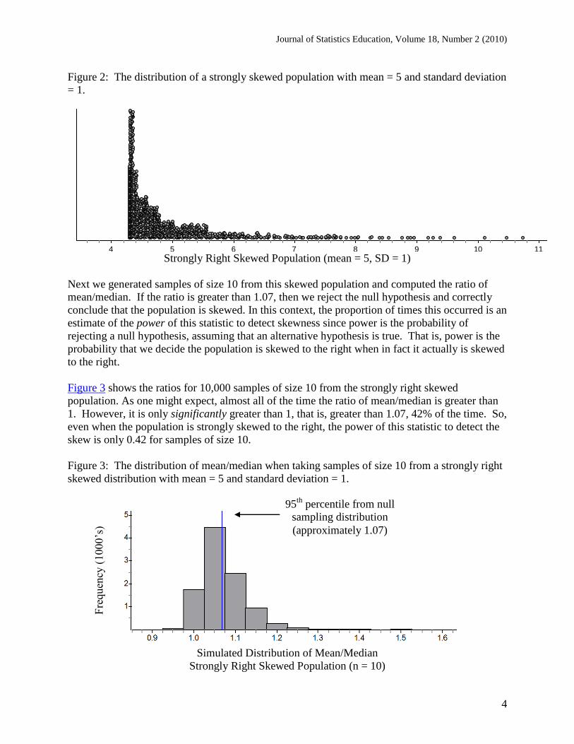
Figure 2: The distribution of a strongly skewed population with mean = 5 and standard deviation

= 1.

chi1

4 5 6 7 8 9 10 11

Collection 1 Dot Plot

Strongly Right Skewed Population (mean = 5, SD = 1)

Next we generated samples of size 10 from this skewed population and computed the ratio of

mean/median. If the ratio is greater than 1.07, then we reject the null hypothesis and correctly

conclude that the population is skewed. In this context, the proportion of times this occurred is an

estimate of the power of this statistic to detect skewness since power is the probability of

rejecting a null hypothesis, assuming that an alternative hypothesis is true. That is, power is the

probability that we decide the population is skewed to the right when in fact it actually is skewed

to the right.

Figure 3 shows the ratios for 10,000 samples of size 10 from the strongly right skewed

population. As one might expect, almost all of the time the ratio of mean/median is greater than

1. However, it is only significantly greater than 1, that is, greater than 1.07, 42% of the time. So,

even when the population is strongly skewed to the right, the power of this statistic to detect the

skew is only 0.42 for samples of size 10.

Figure 3: The distribution of mean/median when taking samples of size 10 from a strongly right

skewed distribution with mean = 5 and standard deviation = 1.

Simulated Distribution of Mean/Median

Strongly Right Skewed Population (n = 10)

95th

percentile from null

sampling distribution

(approximately 1.07)

Fre

quen

cy (

1000

’s)

Journal of Statistics Education, Volume 18, Number 2 (2010)

5

3. Investigating Other Statistics

In the last part of the 2009 investigative task, students were asked to create a new statistic to

measure skewness using only the 5-number summary (the minimum, first quartile, median, third

quartile, and maximum). One of the more popular choices was to compare the distance from Q3

to the maximum to the distance from Q1 to the minimum. Visually, this would be comparing the

right whisker on a boxplot to the left whisker. This could be expressed as a ratio: (max –

Q3)/(Q1 – min) where values greater than 1 would indicate right skewness.

Using the same process as above, 10,000 samples of size 10 were taken from a normal

population with = 5 and = 1 and the value of the ratio (max – Q3)/(Q1 – min) was

calculated. The distribution of this statistic was strongly skewed to the right, with over 99% of

the ratios between 0 and 15. Figure 4 shows the estimated sampling distribution of the ratio

(max – Q3)/(Q1 – min) for these values. The 95th

percentile of this distribution is 5.32, so any

sample that has a ratio of (max – Q3)/(Q1 – min) larger than 5.32 would give convincing

evidence that the population is skewed to the right.

Figure 4: The distribution of (max – Q3)/(Q1 – min) when taking samples of size 10 from

normal population with mean = 5 and standard deviation = 1. Values greater that 15 were

excluded from the graph, but included in the numerical calculations.

Simulated Ratios of (max – Q3)/(Q1 – min)

Normal Population (n = 10)

To measure the power of this statistic, 10,000 random samples of size 10 were taken from the

strongly right skewed population described earlier and the ratio (max – Q3)/(Q1 – min) was

calculated. The distribution of this ratio was extremely skewed to the right, with some ratios

exceeding 200,000. Most of the values, however, were between 0 and 100 as shown in Figure 5.

Fre

quen

cy

95th

percentile

5.32

Journal of Statistics Education, Volume 18, Number 2 (2010)

6

Figure 5: The distribution of (max – Q3)/(Q1 – min) when taking samples of size 10 from a

strongly right skewed distribution with mean = 5 and standard deviation = 1. Values greater that

15 were excluded from the graph, but included in the numerical calculations.

Simulated Ratios of (max – Q3)/(Q1 – min)

Skewed Right Population (n = 10)

Figures 4 and 5 show that most of the values in the simulated distribution of this test statistic

when sampling from a skewed right distribution are above the critical value of 5.32. In fact, of

the 10,000 samples, 85% had ratios that would give convincing evidence that the population is

skewed to the right. The power of this statistic (0.85) is more than twice as big as the

mean/median statistic (0.42), so it appears that (max – Q3)/(Q1 – min) is a much better measure

of skewness in these conditions. Of course, this may not be true if the sample size was changed

or the amount of skewness in the population was altered.

Table 1 shows a list of eleven statistics that were tested using the method described above and

the approximate power they have for detecting skewness when sampling from a distribution that

is strongly skewed to the right. Each statistic was given a name from A to K and then ranked

according to its power. For the statistics A to H, values greater than 1 indicate right skewness.

Fre

quen

cy

95th

percentile from null

sampling distribution

( 5.32)

Journal of Statistics Education, Volume 18, Number 2 (2010)

7

Table 1: The eleven statistics tested, estimates of power when sampling from populations with

different amounts of skewness, ranks and average rank (rank 1 = most power).

Strongly

Skewed

Population

Moderately

Skewed

Population

Slightly

Skewed

Population

Name Statistic Power

(Rank)

Power

(Rank)

Power4

(Rank)

Average

Rank

A mean

median .42 (8) .21 (8) .098 (6) 7.33

B max median

median min

.84 (2) .31 (1) .107 (5) 2.67

C 3

1

Q median

median Q

.28 (9) .10 (9.5) .065 (10) 9.5

D max - Q3

Q1- min .85 (1) .26 (5.5) .090 (7) 4.5

E

1( )

2min+max

median

.56 (5) .30 (2) .126 (1) 2.67

F

1( 1 3)

2Q Q

median

.13 (11) .10 (9.5) .066 (9) 9.83

G

1

21

1 32

(min+max)

(Q +Q )

.49 (6.5) .27 (4) .118 (2) 4.17

H min+Q1+median+Q3+max

5 .49 (6.5) .26 (5.5) .110 (4) 5.33

I

3

3

2

1( )

1( )

x xn

x xn

.68 (3) .28 (3) .113 (3) 3

J 3( )

mean median

standard deviation

.64 (4) .22 (7) .085 (8) 6.33

K 3 ( 1)

3 1

Q median median Q

Q Q

.26 (10) .09 (11) .061 (11) 10.67

Statistics E and G use the midrange, which is the average of the minimum and maximum values

and statistics F and G use the midquartile, which is the average of Q1 and Q3. Statistic H uses

the average of all 5 numbers in the 5-number summary and compares this to the median.

4 Note: Power estimates were given to an additional decimal place to allow for ranking.

Journal of Statistics Education, Volume 18, Number 2 (2010)

8

Statistics I, J and K were included in this investigation since they are standard measures of

skewness. However, statistics I and J would not be acceptable answers on the investigative task

since they require knowing more than just the 5-number summary.

Statistic I is the formal definition of skewness which involves calculating the third moment of

the distribution. Statistic J is often called Pearson’s skewness coefficient and statistic K is called

the quartile skewness coefficient (Weisstein, 2010). All of these statistics should equal 0 in a

symmetric distribution and will be greater than 0 when the distribution is skewed to the right.

One should notice in Table 1 that the statistics have quite a range of power when sampling from

a strongly skewed population. Statistic F had only a 13% chance of detecting the skewness

while statistic D had an 85% chance. Note, also, that the standard measures of skewness do well,

but do not have as much power as statistic B or D.

4. Changing the Amount of Skewness

To investigate these findings more completely, this process was repeated for two other skewed

populations (moderately skewed right and slightly skewed right). Both were randomly generated

from chi-square distributions (df = 5 and df = 40) that were rescaled so that = 5 and = 1.

Figures 6 and 7 provide graphs of 1000 values from each population and show the amount of

skewness these populations contain. Note from Figures 6 and 7 that the distributions become

progressively less skewed and closer to a normal distribution. Thus, we should expect that the

power of each statistic will decrease as well.

Figure 6: The distribution of a moderately right skewed distribution with mean = 5 and standard

deviation = 1.

chi5

3 4 5 6 7 8 9 10 11

Collection 1 Dot Plot

Moderately Right Skewed Population (mean = 5, SD = 1)

Journal of Statistics Education, Volume 18, Number 2 (2010)

9

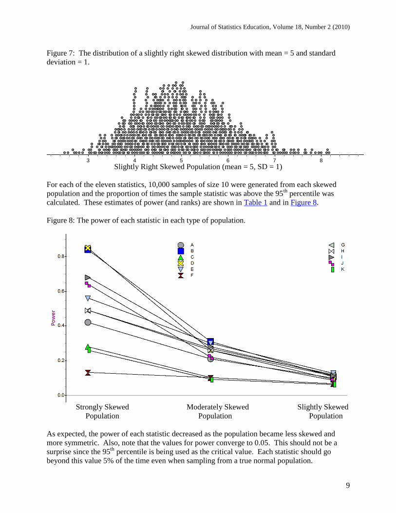
Figure 7: The distribution of a slightly right skewed distribution with mean = 5 and standard

deviation = 1.

chi40

3 4 5 6 7 8 9

Collection 1 Dot Plot

Slightly Right Skewed Population (mean = 5, SD = 1)

For each of the eleven statistics, 10,000 samples of size 10 were generated from each skewed

population and the proportion of times the sample statistic was above the 95th

percentile was

calculated. These estimates of power (and ranks) are shown in Table 1 and in Figure 8.

Figure 8: The power of each statistic in each type of population.

Strongly Skewed Moderately Skewed Slightly Skewed

Population Population Population

As expected, the power of each statistic decreased as the population became less skewed and

more symmetric. Also, note that the values for power converge to 0.05. This should not be a

surprise since the 95th

percentile is being used as the critical value. Each statistic should go

beyond this value 5% of the time even when sampling from a true normal population.

Journal of Statistics Education, Volume 18, Number 2 (2010)

10

Statistic D, which had the most power in the strongly skewed distribution, fell to 7th

place in the

slightly skewed distribution. Statistic B, which was 2nd

initially, fell to 5th

place. Other notable

performances include statistic I, which was consistently in 3rd

place for each degree of skewness;

statistic E, which went from 4th

to 2nd

to 1st; and statistic B, which went from 2

nd to 1

st to 5

th.

Using the average rank as an overall measure of power shown in Table 1, it seems that among

the eleven statistics tested, statistics B and E work best when trying to detect skewness in a

population. Perhaps not coincidentally, both of these involve the same components: the

minimum, median, and maximum.

On the other end of the spectrum, the three worst statistics (C, F and K) all use a combination of

Q1, Q3, and the median. This is probably not too surprising, considering the quartiles ignore the

outer 25% of the distribution where the skewness is most obvious.

5. Sample Classroom Activity #1

The following is an example of an activity that might be used with students to extend the

investigation of skewness and reinforce their understanding of power:

Does the Difference Make a Difference? Choose one of the ratio statistics from the investigation and compare it to the equivalent

difference statistic. For example, compare the ratio mean/median with the difference

mean – median to see if one statistic is more powerful than the other.

1. Generate the null sampling distribution for both statistics by taking random

samples of size 10 from a normal population with = 5 and = 1 and

calculating the values of the statistic.

2. Estimate the 95th

percentiles of each distribution to determine the critical values

for each statistic.

3. For each statistic, take samples of size 10 from a skewed population with = 5

and = 1, compute the value of the statistic from each sample, and calculate

how often the value of the statistic is beyond the critical value from step 2 (the

estimated power).

4. Compare the estimates of power for the ratio and difference statistics.

5. Repeat for different amounts of skewness, as time allows.

To illustrate, Table 2 provides the results for a comparison of the ratio midrange/median (statistic

E) and the difference midrange – median. Although the ratio statistic performed slightly better in

each case, the power estimates were very close. So, it appears that using a difference instead of a

ratio may not make that much difference.

Journal of Statistics Education, Volume 18, Number 2 (2010)

11

Table 2: A comparison of the power to detect skewness between the ratio midrange/median and

the difference midrange – median.

Statistic

Power (Strongly

Skewed Population)

Power (Moderately

Skewed Population)

Power (Slightly

Skewed Population)

Ratio .56 .30 .126

Difference .55 .29 .119

6. Sample Classroom Activity #2

The Role of Sample Size

Does increasing the sample size increase the power of a statistic to detect skewness?

Choose one of the statistics from the investigation and estimate the power using samples

of size 10 and size 100.

1. Generate the null sampling distribution for the statistic using each sample size.

Take random samples of size 10 from a normal population with = 5 and = 1

and calculate the values of the statistic. Then, do the same for samples of size

100.

2. Estimate the 95th

percentiles of each distribution to determine the critical values

for each sample size.

3. Take samples of size 10 from a skewed population with = 5 and = 1,

compute the value of the statistic from each sample, and calculate how often the

value of the statistic is beyond the critical value from step 2 (the power). Repeat

for samples of size 100.

4. Compare the estimates of power for the different sample sizes.

5. Repeat for different amounts of skewness, if time.

To illustrate, Table 3 provides the results using statistic E (midrange/median) for samples of size

10 and samples of size 100. Increasing the sample size definitely increases the power. Of course,

when the sample size is as large as 100, we can generally rely on the central limit theorem when

testing a mean without as much concern about the shape of the population.

Table 3: A comparison of the power to detect skewness for statistic E (midrange/median) with

different sample sizes.

Power (Strongly

Skewed Population)

Power (Moderately

Skewed Population)

Power (Slightly

Skewed Population)

n = 10 .56 .30 .126

n = 100 1.00 .99 .437

Journal of Statistics Education, Volume 18, Number 2 (2010)

12

7. Further Investigations

There are many other possible ways to extend this investigation. For example, do our rankings

stay the same for different sample sizes? What about different population shapes? Could these

same techniques be used to test for heavy tails and not just skewness? Is it possible to determine

any of the values theoretically? Will the ratio and difference statistics always perform similarly?

8. Conclusion

In this paper we have investigated different ways to measure skewness and how to decide which

statistic is the best. Using simulations, we have estimated the power of each statistic to detect

skewness for various population shapes and sample sizes.

These methods, however, are not limited to investigating skewness. For example, when

introducing the standard deviation, students often suggest using the absolute values of the

deviations from the mean rather than squaring the deviations from the mean. A similar

investigation could be used to see which measure more reliably detects an increase in variability.

Students should be encouraged to think creatively about different ways to measure characteristics

of distributions and how to evaluate which one might be best in a given situation.

Acknowledgements

Thanks to the following people for their feedback and suggestions during the development of this

paper: Chris Franklin, Bob Taylor, Ruth Carver, Ken Koehler, Robin Lock, and DV Gokhale. A

version of the paper was presented during the 2009 AP Statistics reading.

References

College Board (2008), Statistics Course Description.

apcentral.collegeboard.com/apc/public/repository/ap08_statistics_coursedesc.pdf

Weisstein, Eric W. "Skewness." From MathWorld--A Wolfram Web Resource.

mathworld.wolfram.com/Skewness.html

Josh Tabor

Canyon del Oro High School

25 W. Calle Concordia

Oro Valley, AZ 85704

Email: joshtabor@hotmail.com

Journal of Statistics Education, Volume 18, Number 2 (2010)

13

Volume 18 (2010) | Archive | Index | Data Archive | Resources | Editorial Board |

Guidelines for Authors | Guidelines for Data Contributors | Home Page | Contact JSE |

ASA Publications