INVESTIGATING THE EXTENT OF DAMAGE

FROM A SINGLE BLASTHOLE

by

Kirk Brandon Erickson

A thesis submitted to the faculty of The University of Utah

in partial fulfillment of the requirements for the degree of

Master of Science

Department of Mining Engineering

The University of Utah

May 2014

Copyright © Kirk Brandon Erickson 2014

All Rights Reserved

The U n i v e r s i t y o f Ut ah G r a d u a t e S c h o o l

STATEMENT OF THESIS APPROVAL

The thesis of Kirk Brandon Erickson

has been approved by the following supervisory committee members:

Michael K. McCarter Chair 6/20/2013Date Approved

Dale S. Preece Member 6/20/2013Date Approved

Paul W. Jewell Member 6/20/2013Date Approved

and by Michael G. Nelson Chair/Dean of

the Department/College/School o f ______________ Mining Engineering

and by David B. Kieda, Dean of The Graduate School.

ABSTRACT

An ever-present challenge at most active mining operations is controlling blast-

induced damage beyond design limits. Implementing more effective wall control during

blasting activities requires (1) understanding the damage mechanisms involved and (2)

reasonably predicting the extent of blast-induced damage. While a common consensus on

blast damage mechanisms in rock exists within the scientific community, there is much

work to be done in the area of predicting overbreak.

A new method was developed for observing near-field fracturing with a

borescope. A field test was conducted in which a confined explosive charge was

detonated in a body of competent rhyolite rock. Three instrumented monitoring holes

filled with quick-setting cement were positioned in close proximity to the blasthole.

Vibration transducers were secured downhole and on the surface to measure near-field

vibrations. Clear acrylic tubing was positioned downhole and a borescope was lowered

through it to view fractures in the grout. Thin, two-conductor, twisted wires were placed

downhole and analyzed using a time-domain reflectometer (TDR) to assess rock

displacement.

Fracturing in the grout was easily observed with the borescope up to 3.78 m (12.4

ft) from the blasthole, with moderate fracturing visible up to 2.10 m (6.9 ft). Measured

peak particle velocities (PPV) at these distances were 310 mm/s (12.2 in./s) and 1,490

mm/s (58.5 in./s), respectively, although no fracturing was observed near the depth of the

vibration transducers located 3.78 m (12.4 ft) from the blasthole. TDR readings were

difficult to interpret but indicated rock displacement in two of the monitoring holes.

Three methods were used to predict the radial extent of tensile damage around the

blasthole: a modified Holmberg-Persson (HP) model, a shockwave transfer (SWT)

model, and a dynamic finite element simulation using ANSYS AutodynTM. The extent of

damage predicted by the HP and SWT models is similar to field measurements when

using static material properties of the rock, but is underestimated using dynamic material

properties. The Autodyn™ model significantly overpredicted the region of damage but

realistically simulated the zones of crushing and radial cracking. Calibration of material

parameters for the AutodynTM model would be needed to yield more accurate results.

iv

ABSTRACT............................................................................................................................ Ill

ACKNOWLEDGEMENTS..................................................................................................vll

1. INTRODUCTION.............................................................................................................. 1

1.1 Blasting in a mining context....................................................................................... 11.2 Blast damage and backbreak....................................................................................... 31.3 Application of blast damage to wall control..............................................................4

2. PREDICTION APPROACHES TO BLAST DAMAGE................................................ 6

2.1 Predicting blast-induced damage................................................................................62.1.1 Vibration............................................................................................................. 82.1.2 Stress and strain................................................................................................232.1.3 Pressure and energy......................................................................................... 242.1.4 Hydrodynamics.................................................................................................272.1.5 Empirical approaches....................................................................................... 282.1.6 Statistics, fuzzy logic, and artificial neural networks....................................292.1.7 Fractal geometry...............................................................................................312.1.8 Numerical methods.......................................................................................... 31

3. EXPERIMENTAL PROCEDURE..................................................................................35

3.1 Equipment summary..................................................................................................353.1.1 Vibration transducers....................................................................................... 363.1.2 Data acquisition................................................................................................473.1.3 Time domain reflectometry.............................................................................483.1.4 Borescope.......................................................................................................... 503.1.5 Quick-setting grout.......................................................................................... 50

3.2 Field experiment setup...............................................................................................503.3 Results.........................................................................................................................59

3.3.1 Vibration records............................................................................................. 593.3.2 TDR results....................................................................................................... 733.3.3 Borescope observations...................................................................................773.3.4 Visual observations.......................................................................................... 813.3.5 Summary of results.......................................................................................... 81

TABLE OF CONTENTS

4. DAMAGE PREDICTION 84

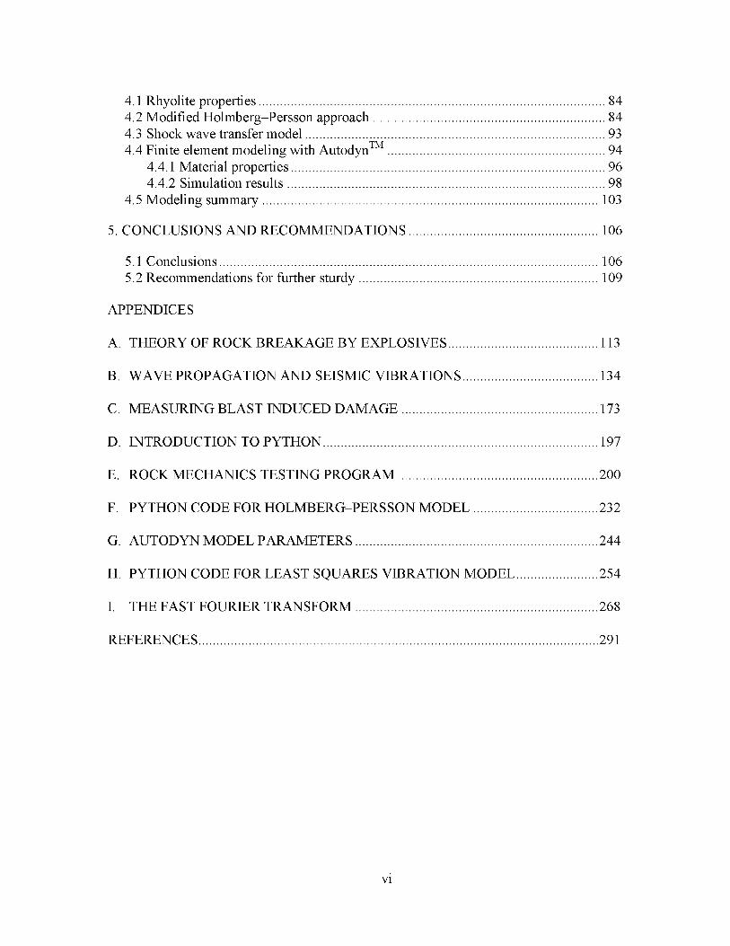
4.1 Rhyolite properties.....................................................................................................844.2 Modified Holmberg-Persson approach................................................................... 844.3 Shock wave transfer model....................................................................................... 934.4 Finite element modeling with Autodyn™............................................................... 94

4.4.1 Material properties........................................................................................... 964.4.2 Simulation results............................................................................................ 98

4.5 Modeling summary..................................................................................................103

5. CONCLUSIONS AND RECOMMENDATIONS.......................................................106

5.1 Conclusions.............................................................................................................. 1065.2 Recommendations for further sturdy..................................................................... 109

APPENDICES

A. THEORY OF ROCK BREAKAGE BY EXPLOSIVES...........................................113

B. WAVE PROPAGATION AND SEISMIC VIBRATIONS.......................................134

C. MEASURING BLAST INDUCED DAMAGE.........................................................173

D. INTRODUCTION TO PYTHON................................................................................197

E. ROCK MECHANICS TESTING PROGRAM..........................................................200

F. PYTHON CODE FOR HOLMBERG-PERSSON MODEL....................................232

G. AUTODYN MODEL PARAMETERS...................................................................... 244

H. PYTHON CODE FOR LEAST SQUARES VIBRATION MODEL.......................254

I. THE FAST FOURIER TRANSFORM...................................................................... 268

REFERENCES.....................................................................................................................291

vi

ACKNOWLEDGEMENTS

This work would not have been possible without assistance from several

individuals. Special thanks to Dr. Michael McCarter, professor of mining engineering, for

originally proposing the idea for my research and serving as my graduate advisor. His

advice, expertise, and tireless efforts were invaluable to the progress of this thesis.

Gratitude is extended to Dr. Paul Jewell, associate professor of geology and geophysics,

and Dr. Dale Preece, senior research fellow with Orica USA Inc., for their willingness to

serve as members of my committee. Additional thanks is made to Dr. Dale Preece for his

recommendations on the Autodyn™ finite element modeling. Sincere appreciation goes

to Robert Byrnes, technician, for his assistance in conducting tests with the triaxial

testing machine and to Hossein Changani, fellow graduate student, in performing tests

with the split Hopkinson pressure bar. Acknowledgement is due for the indiduals at the

mine where the field test was conducted, whose support made this project feasible.

Recognition for financial support is made to the William C. Browning Graduate

Fellowship administered by the University of Utah through the Mining Engineering

Department and to the Best in the West Scholarship administered by the International

Society of Explosives Engineers. Many thanks are owed to encouragement given by

family, friends, student colleagues, and professors who have also been mentors. And last

but not least, I am indebted to the continual, loving support of my parents throughout my

university education and to Providence for guiding me.

1. INTRODUCTION

Rock blasting is a process that has been and continues to be widely used in

mining and civil construction activities. Starting with the incorporation of gunpowder in

the late 17th century and later with the introduction of modern blasting agents with the

creation of dynamite in the 19th century, the use of explosive chemical compounds in

rock breakage applications has become a staple among a wide gamut of mining methods

(Darling 2011). Blasting currently offers the most cost-effective means to reduce rock to

a form that can then be excavated and yet remains acceptably safe when proper controls

are implemented.

1.1 Blasting in a mining context

The primary goal in most production-related blasting activities at a mining

operation is to achieve a target fragmentation size. The size constraints are dictated by

diggability, and in the case of ore, capabilities of downstream comminution activities in

the mine-to-mill path. A significant amount of effort has been and continues to be

dedicated to designing, implementing, and refining blast patterns that will achieve a

desirable fragment size distribution. Three factors primarily control this distribution:

explosive energy quantity, explosive energy distribution, and rock structure (Persson et

al. 1994). While the rock structure cannot be controlled, the other two factors can through

varying a number of pattern design factors. These include the following:

• Explosive type,

• Degree of coupling,

• Hole diameter,

• Hole depth,

• Burden and spacing,

• Stemming,

• Subdrill,

• Timing, and

• Decking.

In addition to achieving fragmentation goals, there are other objectives that the

blasting practitioner must consider:

• Vibration control,

• Wall control,

• Airblast control,

• Flyrock mitigation,

• Abatement of noxious fumes,

• Ore dilution control, and

• Displacement of broken material.

The contribution of each design variable to the outcomes of a particular blast

design can be significant in several ways. Ascertaining the manner and degree of

influence for a variable to arrive at an optimal solution is not always straightforward due

to the complex physical processes that occur during blasting. A change in one parameter,

although intended to alter a characteristic of a blast pattern in a specific manner, may

create unwanted or unintended side effects. For instance, changing the timing scheme on

2

a pattern with hopes of decreasing ore dilution may produce larger ground vibrations.

Increasing stemming to direct a greater portion of the explosive energy into the rock mass

may expand the region of damage beyond the design limits of the blast, adversely

affecting ground integrity and stability.

1.2 Blast damage and backbreak

The detonation of an explosive charge in a solid medium will create what may be

referred to as a zone of damage. In the context of rock breakage by blasting, the extent of

the damaged zone is often referred to as backbreak or overbreak. Within this region of

backbreak, the rock is deemed incompetent due to the damage incurred.

Damage does not have a specific, unique definition—the criteria for delineating

damaged rock apart from sound rock will vary from site to site and even application to

application. For instance, one site may characterize damage as rock that has been

fragmented to the point at which it can be excavated. Another site may label damage as

the formation of large cracks extending into a bench so that unstable features are formed.

Yet another site may classify damage as shifting of rock blocks along preexisting faults

or joint structures.

While there is no one definition of damage, the overall consensus seems to share

common attributes. Oriard (1982) defines damage in his discussion of blasting as

including “not only the breaking and rupturing of rock beyond the desired limits of

excavation but also an unwanted loosening, dislocation, and disturbance of the rock mass

the integrity of which one wishes to preserve.” For the purpose of this thesis, damage in a

rock mass is generally characterized by an increase in both the density and extent of

fractures and similar discontinuities, disturbance and/or weakening of geological features,

3

and an alteration of physical properties such as reduced rock strength or changes in

elastic moduli. Damage also possesses the properties of being cumulative and

irreversible.

The above definition, however, fails to make an important distinction regarding

the scale of damage. Blasting induces damage both on a macroscale and a microscale,

both o f which may be the focus o f different emphases. On the one hand, the geotechnical

engineer is concerned with damage on a macroscale, which manifests itself in the form of

large cracks and unstable blocks that have potential for causing ground instability. On the

other hand, the metallurgical engineer is concerned with damage on a microscale, as

microfractures and reductions in the rock stiffness affect breakage energies during

comminution. The importance of both must be recognized by the blasting engineer. This

work focuses mainly on that which can be observed directly, which is macroscale

damage.

1.3 Application of blast damage to wall control

Before delving into the body of this work, the following question must be

discussed: what is the practical importance o f studying blast-induced damage? Due to the

ubiquitous use of blasting, backbreak is a widespread phenomenon among many mining

operations and certain construction projects. Damaged rock is a contributor to ground

instability. Thus, backbreak is of paramount importance in geotechnlcal analysis and

safety considerations. With regard to structures and buildings, maintaining an intact

foundation when blasting in close proximity can be crucial. For underground excavations,

blasting practices can influence the stability o f openings and dictate the degree of support

needed. At surface mines, implementing good wall control can be a significant task with

4

a large payback. By blasting in a manner that leaves pit slopes competent, batter angles

can be increased and thus, stripping costs are reduced.

Currently, the measurement, quantification, and prediction of backbreak

constitute an area of ongoing extensive research. A better understanding of blast damage

will lead to greater ability in designing better blast patterns and implementing more

effective wall control.

A scientific investigation of blast-induced damage from a single blasthole is here

presented. While the overall scope of this project may appear limited, the collected data

and observations are a valuable contribution to the existing literature on near-field blast

measurements. A new method is presented for directly observing the fracture network

created by the explosive charge. Numerical modeling is conducted to correlate field

measurements associated with blast-induced damage and compare simulation results with

experimental data.

For the reader interested in further study of rock breakage by explosives, vibration

analysis, and measuring blast damage, additional material is provided in the appendices.

A detailed description of theory of rock blasting is presented in Appendix A. Seismic

wave propagation, vibration predictions using the scaled distance concept, and frequency

analysis are reviewed in Appendix B. A summary of methods for measuring blast-

induced damage is given in Appendix C. Since much of the computer programming for

this thesis was done using Python, it was considered appropriate to give a brief

introduction to Python in Appendix D.

5

2. PREDICTION APPROACHES TO BLAST

DAMAGE

In this section, a brief overview of techniques developed for predicting near-field

blast damage will be presented. While numerous, valuable contributions have been made

in these areas towards predicting blasting, only sparse attention will be paid to individual

results. The intent is not to extensively cover these findings, but rather to acquaint the

reader with the variety of approaches that have been attempted. References made in

regards to each approach are meant to provide an example from literature, in lieu of an

all-inclusive compilation. Only items of pertinent interest to research efforts later in this

thesis will be discussed in detail.

2.1 Predicting blast-induced damage

An extensive body of literature exists on endeavors to quantitatively predict the

limits of blast-induced damage. Approaches developed encompass everything from

simple analytical expressions and rules of thumb to advanced analytical expressions and

numerical models. While a consensus exists within the scientific community regarding

the common damage mechanisms that occur during blasting, little consensus exists on

how to appropriately predict backbreak. As is discussed in Appendix A, explosive-

induced rock breakage involves the interaction of several complex physical phenomenon.

In developing a prediction method, the tendency is to make certain simplifying

assumptions in hopes that the overall solution will not be detrimentally affected.

Oversimplification easily results, however, particularly with analytical expressions. With

the continual advances in computational ability using computers, numerical methods

offer a means for incorporating high model complexity and coupled interactions while

staying true to fundamental laws regarding conservation of mass, momentum, and

energy. However, a numerical simulation is only as good as its input parameters,

constitutive material models, and equations of state. Numerical methods are also subject

to additional constraints and sources of error such as floating point precision,

computational stability, and numerical artifacts that can occur (i.e., element errors,

boundary effects, solution nonconvergence, and limited model resolution).

Most nonnumerical prediction methods tend to focus only on one or two key

variables in the blasting process. Thus, selection of a method requires considering the

variables of choice. This is particularly true when comparing computational results to

field measurements.

In a comparative review of several damage limit models, Iverson et al. (2010)

posed a set of key issues that needs to be addressed in backbreak prediction. Several of

these are listed here, for not only are they applicable to most damage models, but they

have potential to significantly affect the outcome. Among them are

• Deciding on a definition or definitions of damage in a blasting

environment;

• Knowing how to best measure damage;

• Determining what variables should be used in calculating damage, such as

gas pressure, wave energy, etc.;

• Determining whether quasistatic or dynamic assumptions are appropriate;

7

• Knowing whether to use static or dynamic properties of rocks, and how to

best measure them, especially dynamics properties; and

• Determining if basic explosive properties are sufficient.

Hand-in-hand with backbreak prediction is fragmentation prediction. The two

fields are often treated separately in the modeling process, but the breakage mechanisms

involved are the same. While the following summary of prediction approaches focuses on

blast damage limits, some of these tools may well have usefulness in predicting

fragmentation.

With everything said, there is one additional benefit o f modeling to keep in mind.

Hustrulid (1999) makes the valid point that even if a model or simulation does not reflect

the physics o f the real world as accurately as hoped, it may still lend itself useful for

comparative studies. As long as a damage prediction tool produces reasonable results, it

can provide the blasting practitioner or researcher with information regarding relative

changes between, say, blast designs or field conditions.

The following list o f methods for predicting the extent o f blast-induced damage

represents those encountered during a fairly extensive review of literature. Some

techniques have been utilized extensively, while others have only a marginal presence or

have only recently been developed. The author has attempted to cite those contributions

that seem to be most relevant.

2.1.1 Vibration

Perhaps the most common prediction tool o f all is damage limits based on

vibration. Predictions of near field vibrations have ranged from empirical correlation of

site-specific limits to variations using scaled distances to advanced analytical solutions.

8

2.1.1.1 Usefulness of vibration as a predictor

The reasons why vibration has attained a broad presence in damage prediction are

threefold, in the author’s estimation.

1. The practice of recording blast-induced vibrations makes damage criteria

via vibration a natural choice. A sizeable body of experimental data is

available in this area.

2. As discussed in Section C.1.1 in Appendix C, vibration measurements

either record strain directly or can be easily converted to strain or strain

rate using the mechanical properties o f the medium through which the

seismic wave is passing. The relationships are (Yang et al. 1993)

9

du du dt 1 dx dt dx c

dv dv dt 1 dx dt dx c

(2.1)

(2.2)

where

e and e are the strain and strain rate, respectively,

is the particle displacement,

is the particle velocity,

is the particle acceleration,

t is the time from detonation of the explosive charge,

c is the seismic wave velocity, usually equal to the P-wave velocity cP,

and

x = c t is the distance from the explosive charge.

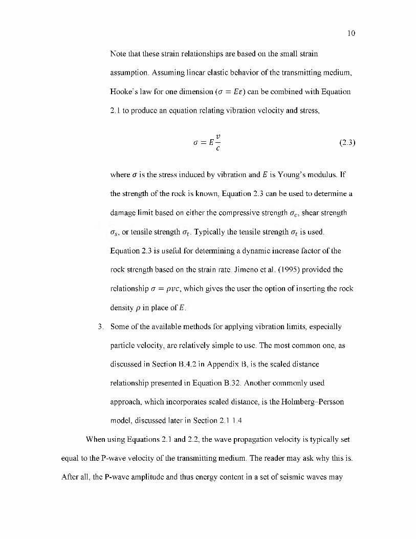
Note that these strain relationships are based on the small strain

assumption. Assuming linear elastic behavior of the transmitting medium,

Hooke’s law for one dimension ( a = Ee) can be combined with Equation

2.1 to produce an equation relating vibration velocity and stress,

va = E — (2.3)

c

where a is the stress induced by vibration and E is Young’s modulus. If

the strength of the rock is known, Equation 2.3 can be used to determine a

damage limit based on either the compressive strength , shear strength

, or tensile strength . Typically the tensile strength is used.

Equation 2.3 is useful for determining a dynamic increase factor of the

rock strength based on the strain rate. Jimeno et al. (1995) provided the

relationship a = pvc, which gives the user the option of inserting the rock

density in place of .

3. Some of the available methods for applying vibration limits, especially

particle velocity, are relatively simple to use. The most common one, as

discussed in Section B.4.2 in Appendix B, is the scaled distance

relationship presented in Equation B.32. Another commonly used

approach, which incorporates scaled distance, is the Holmberg-Persson

model, discussed later in Section 2.1.1.4.

When using Equations 2.1 and 2.2, the wave propagation velocity is typically set

equal to the P-wave velocity of the transmitting medium. The reader may ask why this is.

After all, the P-wave amplitude and thus energy content in a set of seismic waves may

10

not be the largest component. Furthermore, since P-waves possess the largest velocity of

all seismic wave velocities, dividing the particle velocity by would seem to give a

smaller value of strain than if using the S-wave ( cs) or Raleigh wave velocities ( cR). The

reasons apparent to the author are

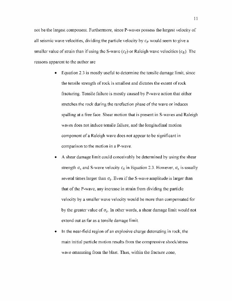
• Equation 2.3 is mostly useful to determine the tensile damage limit, since

the tensile strength of rock is smallest and dictates the extent of rock

fracturing. Tensile failure is mostly caused by P-wave action that either

stretches the rock during the rarefaction phase of the wave or induces

spalling at a free face. Shear motion that is present in S-waves and Raleigh

waves does not induce tensile failure, and the longitudinal motion

component of a Raleigh wave does not appear to be significant in

comparison to the motion in a P-wave.

• A shear damage limit could conceivably be determined by using the shear

strength <rs and S-wave velocity cs in Equation 2.3. However, <rs is usually

several times larger than <rt . Even if the S-wave amplitude is larger than

that of the P-wave, any increase in strain from dividing the particle

velocity by a smaller wave velocity would be more than compensated for

by the greater value of . In other words, a shear damage limit would not

extend out as far as a tensile damage limit.

• In the near-field region of an explosive charge detonating in rock, the

main initial particle motion results from the compressive shock/stress

wave emanating from the blast. Thus, within the fracture zone,

11

longitudinal wave motion dominates, and the most favorable failure mode

from ground response beyond the crushing zone is tensile.

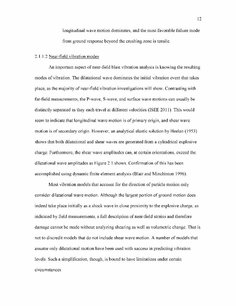
2.1.1.2 Near-field vibration modes

An important aspect of near-field blast vibration analysis is knowing the resulting

modes of vibration. The dilatational wave dominates the initial vibration event that takes

place, as the majority of near-field vibration investigations will show. Contrasting with

far-field measurements, the P-wave, S-wave, and surface wave motions can usually be

distinctly separated as they each travel at different velocities (ISEE 2011). This would

seem to indicate that longitudinal wave motion is of primary origin, and shear wave

motion is of secondary origin. However, an analytical elastic solution by Heelan (1953)

shows that both dilatational and shear waves are generated from a cylindrical explosive

charge. Furthermore, the shear wave amplitudes can, at certain orientations, exceed the

dilatational wave amplitudes as Figure 2.1 shows. Confirmation of this has been

accomplished using dynamic finite element analysis (Blair and Minchinton 1996).

Most vibration models that account for the direction of particle motion only

consider dilatational wave motion. Although the largest portion of ground motion does

indeed take place initially as a shock wave in close proximity to the explosive charge, as

indicated by field measurements, a full description of near-field strains and therefore

damage cannot be made without analyzing shearing as well as volumetric change. That is

not to discredit models that do not include shear wave motion. A number of models that

assume only dilatational motion have been used with success in predicting vibration

levels. Such a simplification, though, is bound to have limitations under certain

circumstances.

12

13

Figure 2.1 Resultant P-wave and S-wave amplitude potentials from a cylindrical charge (Source: Heelan 1953. Reprinted with the permission of the Society of Exploration

Geophysicists).

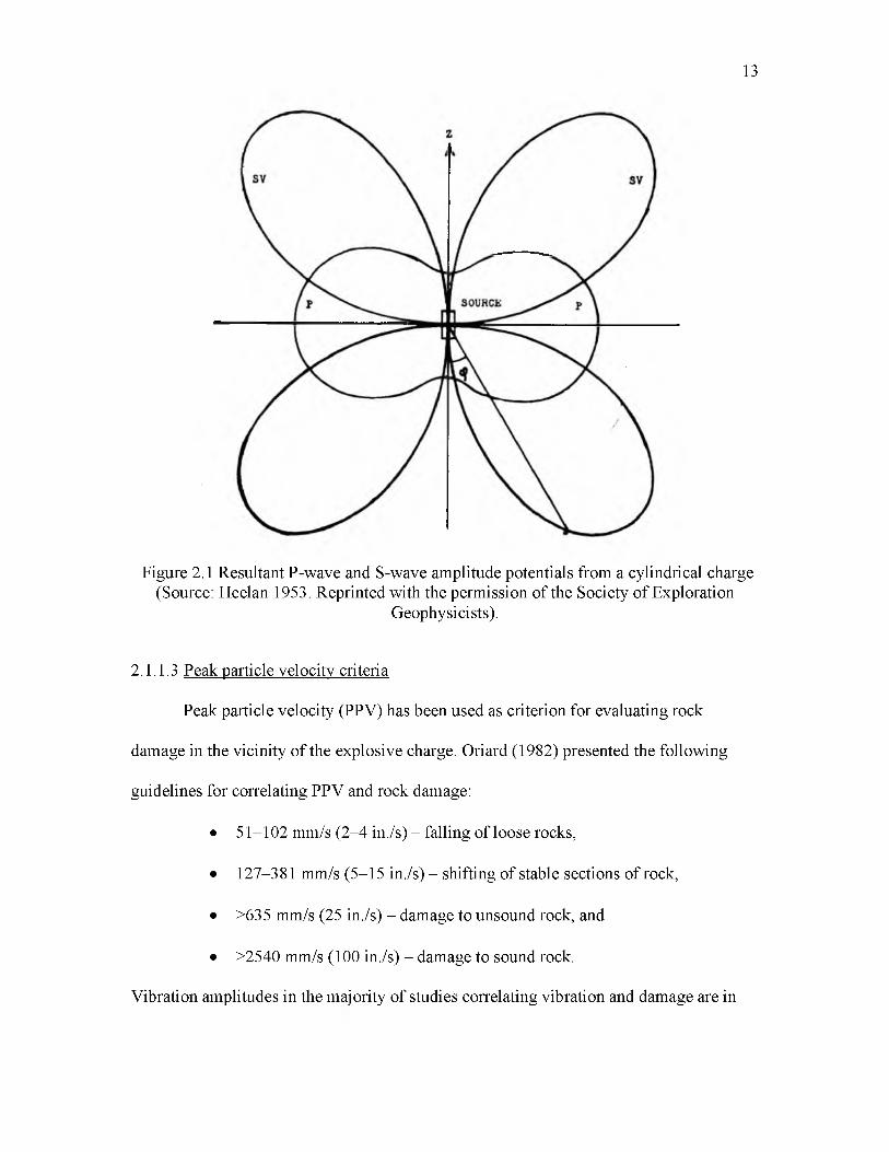
2.1.1.3 Peak particle velocity criteria

Peak particle velocity (PPV) has been used as criterion for evaluating rock

damage in the vicinity of the explosive charge. Oriard (1982) presented the following

guidelines for correlating PPV and rock damage:

• 51-102 mm/s (2-4 in./s) - falling of loose rocks,

• 127-381 mm/s (5-15 in./s) - shifting of stable sections of rock,

• >635 mm/s (25 in./s) - damage to unsound rock, and

• >2540 mm/s (100 in./s) - damage to sound rock.

Vibration amplitudes in the majority o f studies correlating vibration and damage are in

this general range. When using PPV as an indicator o f damage, distinctions need to be

made as to what kinds o f damage correspond with each vibration level, as there are

multiple modes of rock failure. Figure 2.2 shows one such comparison by McKenzie and

Holley (2004) from a field study. A large quantity of research has been conducted using

PPV. For the interested reader, a sample o f field studies is listed as follows: Adamson

and Scherpenisse (1998), Dey and Murthy (2013), LeBlanc et al. (1996), Liu et al.

(1998), Murthy et al. (2004), Rorke and Mllev (1999), and Yang et al. (1993).

In order to correlate PPV and damage, there needs to be a technique in place to

interpolate vibrations. The next section will present some approaches that have been

developed.

14

Figure 2.2 Field measurements correlating peak particle vibrations and damage intensity (Source: McKenzie and Holley 2004. Reprinted with the permission of the International

Society of Explosives Engineers).

15

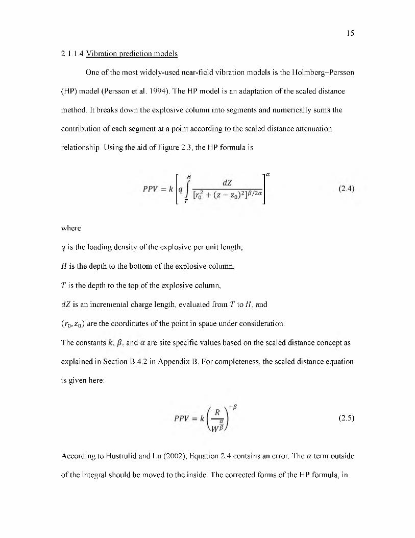
2.1.1.4 Vibration prediction models

One of the most widely-used near-field vibration models is the Holmberg-Persson

(HP) model (Persson et al. 1994). The HP model is an adaptation of the scaled distance

method. It breaks down the explosive column into segments and numerically sums the

contribution of each segment at a point according to the scaled distance attenuation

relationship. Using the aid of Figure 2.3, the HP formula is

where

q is the loading density of the explosive per unit length,

H is the depth to the bottom of the explosive column,

T is the depth to the top of the explosive column,

dZ is an incremental charge length, evaluated from T to H, and

(r0 , z0 ) are the coordinates of the point in space under consideration.

The constants , , and are site specific values based on the scaled distance concept as

explained in Section B.4.2 in Appendix B. For completeness, the scaled distance equation

is given here:

According to Hustrulid and Lu (2002), Equation 2.4 contains an error. The a term outside

of the integral should be moved to the inside. The corrected forms of the HP formula, in

H a

T

(2.5)

16

Figure 2.3 Schematic of Holmber-Persson near-field vibration model After Persson et al. (1994).

17

both integral and discrete formulations, are

H adZ

(2.6)PPV = kq a I I p_t \[r02 + (z - z0) 2 ]2 a

a

PPV = k q a y (2.7)

The HP model has been used with varying degrees of success. Its popularity lies

in its incorporation of the widely-used scaled distance concept and its relative ease of

enhance its accuracy (Arora and Dey 2013; Iverson et al. 2008; Smith 2003). Figure 2.4

shows a typical set of vibration contours generated by the HP model around a blasthole.

There are a few items of concern that have been brought forth, however (Blair and

Minchinton 1996; Ouchterlony et al. 2001). Chief among these are the manner in which

charge increments are summed. No attempt is made either to (1) account for differences

in arrival of the strain pulse originating from each charge increment or (2) resolve into

components each arrival based on its incoming direction. Regarding the first issue,

Persson et al. (1994) claimed that the peak particle velocity does not occur when the

wavefronts arrive, but when the rock mass as a whole starts to move. Thus, the difference

in arrival times are insignificant compared to the timescale of rock motion. Regarding the

second issue, a case study by Arora and Dey (2013) claimed improved results when

resolving individual velocity vectors and then calculating a resultant net velocity.

However, Blair and Minchinton (1996) argued that superposition of the incremental

implementation. Several modifications of the HP model have also been proposed to

18

Figure 2.4 Vibration contours in mm/s generated by the HP model around a singleblasthole

charges does not solve a fundamental issue of vibrations from different wave types. Both

dilatational and shear waves originate from a cylindrical charge, but the HP model does

not distinguish between the two. Thus, the usual assumption is that all vibrations are from

longitudinal wave motion.

The HP also assumes instantaneous detonation of the explosive column. As

pointed out by Blair and Minchinton (1996), even more accurate solutions such as that

developed by Heelan (1953) can err from this assumption when compared to numerical

simulations that incorporate a finite velocity of detonation.

One of the earlier analytical solutions to blast-induced vibrations was developed

by Favreau (1969). Favreau calculated elastic solutions for strains and vibrations from an

explosive charge within a spherical cavity. His work later became the basis for vibrations

models developed by Harries (1983) and Hustrulid’s CSM model (Hustrulid and Lu

2002).

As has been mentioned earlier, Heelan (1953) calculated elastic solutions for

vibrations from a cylindrical explosive charge in terms of two displacement potentials.

His work was later modified by Abo-Zena (1977), who found errors in Heelan’s work.

However, the differences are miniscule (Hustrulid and Lu 2002). Heelan (1953) came to

the interesting result that as much as 60% of the seismic energy from near-field vibrations

is comprised of shear waves, and only 40% dilatational waves. Heelan’s solution,

however, requires the pressure function applied to the wall of the cavity to be assumed,

limiting its theoretical soundness (Hustrulid and Lu 2002). Instantaneous detonation of

the explosive column is implied.

Jordan (1962) solved the case for a cylindrical explosive column with a finite

detonation velocity in an elastic medium. He made the observation that during the peak

compressive phase of the outgoing dilatational phase, the elastic solution indicates all

three of the stress components (radial, tangential, and axial) are compressive. This brings

into question the commonly-accepted tensile “hoop stress” phenomenon that occurs in

the radial fracture zone as discussed in Section A.2 in Appendix A. Jordan states

* n (b (bA potential function is a function that satisfies Lapaces equation V z p = = 0. With potential

functions, irrotational motion is assumed. Potential functions can be used to establish equipotential, or

constant, lines of a quantity such as velocity.

19

that this tensile phase instead occurs near the tail-end of the outgoing strain pulse, and

that all three stress states are tensile at the same time.

A number of studies were conducted by the U.S. Bureau of Mines on strain wave

decay from “approximately spherical” charges in Lithonia granite (for examples, see

Atchison and Pugliese 1964; Atchison and Roth 1961; Atchison and Tournay 1959;

Duvall and Petkof 1959; Fogelson et al. 1959). By “approximately spherical,” the charges

were actually cylindrical with length-to-diameter ratios of less than eight (Hustrulid

1999). Strain gauges were bonded to rock cores and secured downhole with cement.

Strain measurements from different explosives and at different distances were obtained,

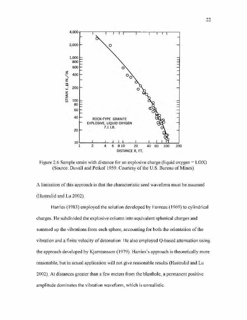
such as those shown in Figure 2.5. The exponential or power attenuation laws described

in Equations B.13 and B. 14 in Appendix B were fit to the data. Figure 2.6 shows one

such plot. In one report, a comparison was made between strain energy and distance

(Fogelson et al. 1959). Scaling was also performed according to both distance and charge

weight so comparisons could be made between different distances and charges.

Starfield and Pugliese (1968) developed the seed waveform model for simulating

cylindrical charges that is easily implemented and can return quite reasonable results

(Hustrulid 1999; Hustrulid and Lu 2002). Like the HP model, the explosive column is

subdivided into charge increments. A seed waveform is assumed for each increment, and

the results are summed up at a point to give the overall vibration history. A finite

detonation velocity is accounted for. Starfield and Pugliese (1968) used idealized strain

seed waveforms based on experimentally obtained strain data from the U.S. Bureau of

Mines. These seed waveforms were resolved using simplified strain rotation formulas.

20

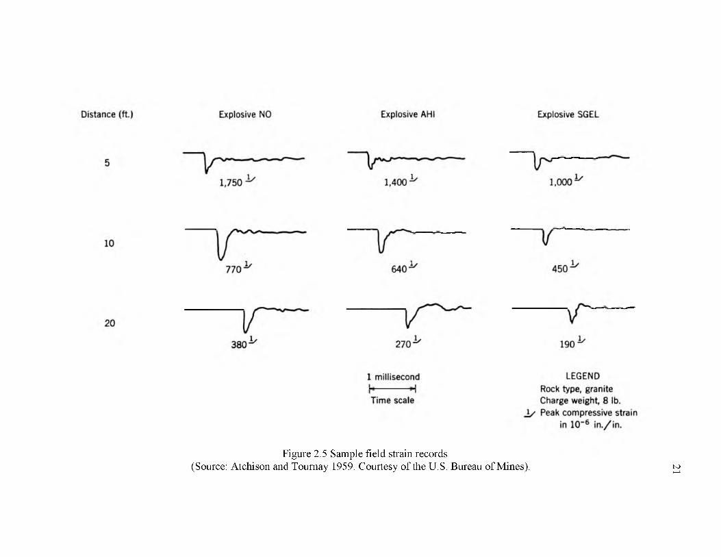
Figure 2.5 Sample field strain records (Source: Atchison and Tournay 1959. Courtesy of the U.S. Bureau of Mines). 21

22

Figure 2.6 Sample strain with distance for an explosive charge (liquid oxygen = LOX) (Source: Duvall and Petkof 1959. Courtesy of the U.S. Bureau of Mines).

A limitation of this approach is that the characteristic seed waveform must be assumed

(Hustrulid and Lu 2002).

Harries (1983) employed the solution developed by Favreau (1969) to cylindrical

charges. He subdivided the explosive column into equivalent spherical charges and

summed up the vibrations from each sphere, accounting for both the orientation of the

vibration and a finite velocity of detonation. He also employed Q-based attenuation using

the approach developed by Kjarntansson (1979). Harries’s approach is theoretically more

reasonable, but in actual application will not give reasonable results (Hustrulid and Lu

2002). At distances greater than a few meters from the blasthole, a permanent positive

amplitude dominates the vibration waveform, which is unrealistic.

Hustrulid’s CSM model (Hustrulid and Lu 2002) also employs the solution

developed by Favreau (1969) to cylindrical charges by subdividing the explosive column

into spheres. Instead of summing the resulting vibrations from each charge increment like

Harries did, Hustrulid concluded that the duration of the initial strain pulse is sufficiently

short that there is no need to perform superposition of the vibrations. Thus, only radial

PPVs are accounted for.

Hustrulid and Lu (2002) developed a hybrid approach which combines together

Heelan’s (1953) elastic solutions, a pressure function proposed by Blair and Minchinton

(1996), and the scaled distance formulation. The hybrid approach closely approximates

the HP model under certain condition, but compares reasonably well with a finite

difference simulation performed using Itasca’s FLAC® software, using the same input

pressure function.

2.1.2 Stress and strain

Stress, strain, vibration, and energy are closely related to each other. Thus, some

of the models discussed in Sections 2.1.1.4 and 2.1.3 could very well be included here.

Using stress or strain as a damage predictor requires the use of a failure model. A

plethora of failure models exist, ranging from popular rock mechanics failure criteria

such as Mohr-Coulomb and Hoek-Brown to advanced models such as the RHT (Reidel

et al. 1999) and JH2 (Johnson and Holmquist 1993) models which are usually only

employed with numerical methods. In addition, several models have been developed

specifically for blasting. For specific examples see Hamdi et al. (2011), Liu and

Katsabanis (1997), Yang et al. (1996), Yang et al. (2002), and Yang and Wang (1996).

All of these models include a damage accumulation mechanism. Since there is an

23

extensive body of literature on various failure models, a discussion of these is not

included here.

Drukovanyi et al. (1976) derived boundaries for the crushing and radial fissuring

zones for a cylindrical charge. They used an analysis of quasistatic gas pressures within

an expanding borehole cavity. A comparison with published field data indicates the

approach produces comparative results (Drukovanyi et al. 1976). A laboratory study by

Iverson et al. (2010) indicated, however, that the model developed by Drukovanyi et al.

(1976) slightly underestimates the zone of crushing and significantly overestimates the

extent of radial fractures.

An approach for estimating zones of rock mass damage from decay of the

shock/stress wave was presented by Atchison et al. (1964). Three zones were identified

as shown in Figure 2.7: (1) the source zone where high pressure gases from the explosive

reaction expand and impact the borehole wall, (2) the transition zone where crushing and

fracturing of the rock occurs, and (3) the seismic or undamaged zone. Johnson (2010)

expanded the number of regions to five, separating the source zone into the explosive and

the decoupled zones and the transition zone into crushing and radial fracture zones.

Johnson also developed a modification of the split Hopkinson bar called the Hustrulid bar

for measuring these regions of decay in rock samples.

2.1.3 Pressure and energy

Several pressure and energy-based models have been developed by considering

the interaction between the gas-induced borehole pressure on the blasthole walls. Some

are based on empirical rules, others on a more rigorous analysis of the thermodynamics

and material physics involved. A few of these are presented below.

24

25

Figure 2.7 Zones of damage for a decoupled charge (Source: Atchison et al. 1964. Courtesy of the U.S. Bureau of Mines).

Hustrulid and Johnson (2008) developed a pressure-based methodology for

estimating the radius of damage in drift rounds. The end result, as originally derived by

Hustrulid (1999), is

Rd_ _ 2^ PesANFO 2.65

r h A PANFO J Prock(2.8)

where

is the radius of damage in the surrounding rock,

is the diameter of the blasthole,

is the density of the explosive,

sAnfo is the relative weight strength of ANFO,

Pa NF0 is the density of ANFO, and

Prock is the density of the rock.

Ouchterlony (1997) considered both the pressure-based behavior of the gaseous

explosive products and the properties of the rock to arrive at a set of formulas that

incorporate the following parameters:

• Explosive density, velocity of detonation (VOD), and adiabatic expansion

constant;

• Borehole diameter and coupling ratio between the explosive and borehole

walls; and

• Rock density, acoustic velocity, and fracture toughness.

Comparing with experimental results, Ouchterlony’s predictions are reasonable with low-

VOD explosives, but do not hold up well with high-VOD explosives (Ouchterlony 1997).

Bastante et al. (2012) developed a blast-induced damage similar to those of

Hustrulid and Johnson (2008) and Ouchterlony (1997), but with only three parameters

needed. These parameters are

• Explosive energy of the charge,

• Coupling factor and rock constant between the explosive and rock, and

• Mean gas isentropic expansion factor.

Comparison of this prediction method with published field data indicates a reasonably

good fit (Bastante et al. 2012).

Sun (2013) developed a shock wave transfer (SWT) model that attempts to

theoretically account for the gas-rock interaction. By using Hugoniot relationships for

26

both the explosive and the rock and enforcing force and velocity continuity between the

two, the gas pressure on the borehole wall is estimated. The response of the rock is

divided into two regions: a crushing zone and a tensile cracking zone. The size of each

zone is dictated by the dynamic compressive and tensile strengths, respectively, of the

rock. When entering static strengths, a dynamic increase factor is applied. Both fully

coupled and decoupled charges are considered. For decoupled charges, the interaction

between the explosive and air is accounted for using a Hugoniot relationship before

determining the combined effect on the borehole wall. Sun compared his model with

multiple blast damage models and types of field data, both published by others and his

own set of tests at a mine. There was reasonable agreement with the SWT model in

almost every case. However, Sun’s own laboratory experiments, in which explosive

charges of different sizes were detonated inside a cast concrete cylinder, did not produce

satisfactory results. Sun attributed this to the small scale of the laboratory experiment, in

which a free face was present in close vicinity to the charge.

2.1.4 Hydrodynamics

Hydrodynamics is a subset of fluid mechanics that concerns the motion of liquids

(National Oceanic and Atmospheric Administration [NOAA] n.d.). Hydrodynamic

approaches to predicting the motion of a body of rock subject to blast loading have been

pioneered by researchers within the Russian scientific community (Hustrulid 1999). Most

prominent among these are a series of papers by Neiman (1979, 1983, 1986).

Hydrodynamics models use principles from fluid mechanics to develop velocity potential

functions that describe the rock motion. They are advantageous in that the effects such as

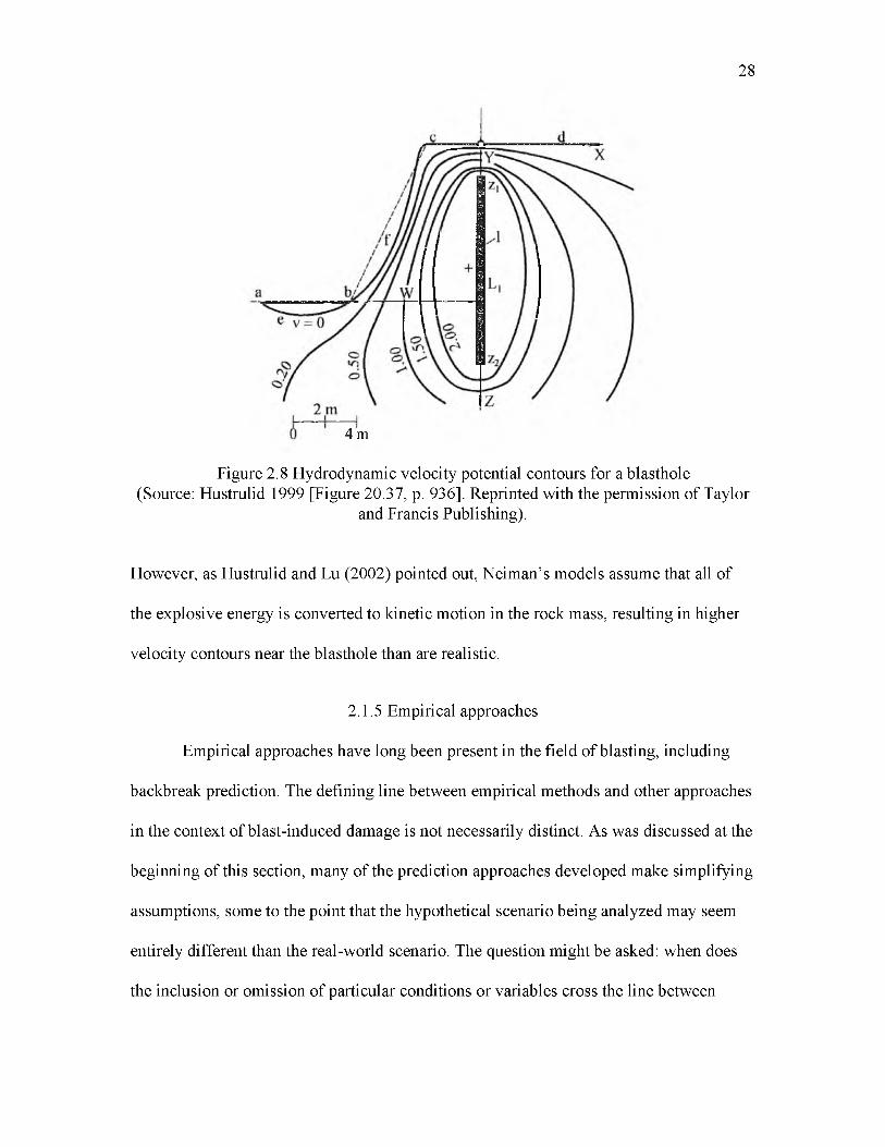
free face and additional blastholes can be accounted for, as exhibited in Figure 2.8.

27

28

4 m

Figure 2.8 Hydrodynamic velocity potential contours for a blasthole (Source: Hustrulid 1999 [Figure 20.37, p. 936]. Reprinted with the permission of Taylor

and Francis Publishing).

However, as Hustrulid and Lu (2002) pointed out, Neiman’s models assume that all of

the explosive energy is converted to kinetic motion in the rock mass, resulting in higher

velocity contours near the blasthole than are realistic.

2.1.5 Empirical approaches

Empirical approaches have long been present in the field of blasting, including

backbreak prediction. The defining line between empirical methods and other approaches

in the context of blast-induced damage is not necessarily distinct. As was discussed at the

beginning of this section, many of the prediction approaches developed make simplifying

assumptions, some to the point that the hypothetical scenario being analyzed may seem

entirely different than the real-world scenario. The question might be asked: when does

the inclusion or omission of particular conditions or variables cross the line between

maintaining a reasonable level of theoretical soundness and becoming an empirical

method? That question is not answered here, but merely presented as food for thought.

The formula for scaled distance presented in Equation 2.5 is, for all intents and

purposes, an empirical approach. Thus, it might be said that any method based on the

scaled distance concept is inherently empirical. However, a number of models with

certain levels of theoretical rigorousness have been developed in conjunction with scaled

distance.

A number of simplistic empirical approaches (i.e., “rules of thumb”) have been

proposed, some with specialized applications in mind. LeBlanc et al. (1996) gave a list of

several of these. A frequent characteristic is that only one or two variables are needed in

the formulation; hence, they are labeled as simplistic. As an example, Ouchterlony et al.

(2001) discussed recommendations made by the Swedish National Road Administration

for cautious blasting. The equations to generate blasting tables use only one variable: the

charge weight. Ouchterlony et al. (2001) discussed the need for incorporating other

factors such as water, coupling, rock properties, and so forth. Clearly, an approach that

could incorporate such factors yet remain accessible to the nonmathematically inclined

user would require an empirical approach.

2.1.6 Statistics, fuzzy logic, and artificial neural networks

In recent years, blasting technologies have begun incorporating tools such as

fuzzy logic and artificial neural networks (ANN). Fuzzy logic is a mathematical

reasoning tool that does not evaluate in terms of absolute values, such as true and false,

but rather in “partial truths” defined by membership functions. Fuzzy logic has

applications where possibilities lie in more than one state, or when linguistic terms are

29

incorporated (Monjezi et al. 2009). ANN are essentially pattern recognition algorithms

that can be programmed so a machine or computer can “learn.” ANN architecture has

been employed within the mining industry in expert control systems for monitoring

processes that require the system to analyze feedback and adapt to changes. These

approaches have been tested in backbreak prediction with increasing degrees of success

over traditional statistical tools. Some examples are provided below.

Singh et al. (2008) compared prediction abilities between traditional multivariate

regression analysis (MVRA) and a neuro-fuzzy interface system to estimate both PPV

and frequency content in blast vibrations. The neuro-fuzzy interface significantly

outperformed MVRA. Two studies comparing MVRA with ANN produced similar

results, with the ANN predicting blast vibration outcomes with much greater accuracy

(Alvarez-Vigil et al. 2012; Khandelwai and Singh 2009). In a third study by Rathore et al.

(2013) comparing MVRA and ANN in vibration amplitude and frequency prediction, the

results were similar. However, their ANN model achieved higher correlation

coefficients of 0.999 and 0.994 in predicting PPV and frequency, respectively, compared

to 0.981 and 0.940 for the regression model. Dehghani and Ataee-pour (2011) conducted

a study comparing ANN against various scaled distance formulations for vibration

prediction. The correlation coefficient of the ANN vibration predictions was higher than

any of the other methods.

Backbreak prediction has been performed using both fuzzy logic and MVRA.

Monjezi et al. (2009) used both fuzzy theory and MVRA to predict backbreak limits at a

mine. The fuzzy approach gave an R2 correlation coefficient of 0.95, versus 0.34 for

MVRA. Mohammadnejad et al. (2013) applied MVRA using a support vector machine

30

(SVM) learning algorithm for predicting backbreak. Over a study of 193 data sets, the

SVM algorithm achieved an R2 correlation coefficient of 0.94.

2.1.7 Fractal geometry

Fractal geometry is a subset of chaos theory in mathematics in which seemingly

random patterns have the property of being self-similar, meaning that they appear the

same regardless of scale (Stewart 2002). Fractal geometry has been gaining presence in a

number of scientific fields of study including rock mechanics and geological

investigations. The literature on applications of fractal geometry to the field of blasting is

scant, but slowly gaining a presence. A couple of fractal damage models have already

been presented (Yang and Wang 1996; Qian and Hiu 1997). Lu and Latham (1999)

presented a rock blastability criterion using the fractal dimension of in situ block sizes. It

is the author’s opinion that the application of fractal geometry to backbreak prediction

presents an interesting study with significant potential. Fractal geometry has the potential

to better describe the random progression of crack growth in rock than other methods

employed in fracture mechanics.

2.1.8 Numerical methods

Numerical methods for analyzing physical processes have become increasingly

popular over the past few decades. In addition to being able to perform simulations of

phenomenon beyond the abilities of analytical and empirical approaches, numerical

methods provide detailed insight into physical quantities not easily measurable in

laboratory and field tests. The most common numerical modeling formulations are finite

difference methods (FDM), finite element methods (FEM), boundary element methods

31

(BEM), and discrete element methods (DEM). In addition to these exist a large number of

other numerical approaches, as well as coupled or hybrid methods. Each method has its

advantages and disadvantages in terms of complexity, computational requirements,

robustness in adapting to different scenarios, modeling setup considerations, and so forth.

Several companies such as ANSYS, COMSOL, SIMULIA, and Itasca make a wide

variety of commercial modeling software packages. In addition, a number of free

programs are available for limited or specialized modeling applications.

The literature on numerical modeling of blasting with regard to damage is quite

extensive. Only a couple of the more prominent studies will be covered here.

A coupled numerical modeling tool currently under development at the writing of

this thesis is the Hybrid Stress Blasting Model (HSBM) (Furtney et al. 2010; Hustrulid et

al. 2009; Onederra et al. 2010; Onederra et al. 2013a, 2013b). The HSBM employs a

detonation model and a rock breakage engine comprised of three parts: (1) a continuum

model for near-field rock response, (2) a brittle discrete element model that can fracture

into “pieces” and move, and (3) a gas product model that can simulate burden movement

under acceleration from high-pressure gas expansion (Onederra et al. 2013b). The Mohr-

Coulomb failure model is used in both the continuum and DEM components (Onederra et

al. 2013a). The near-field continuum mesh uses Itasca’s FLAC® finite difference code.

The DEM model uses a simplified version of Itasca’s PFC3D® DEM code that accounts

only for translation of particles and neglects rotation. Laboratory-scale tests have been

conducted comparing HSBM predictions to measured damage in instrumented concrete

blocks, as shown in Figure 2.9 (Onederra et al. 2010; Onederra et al. 2013a, 2013b).

32

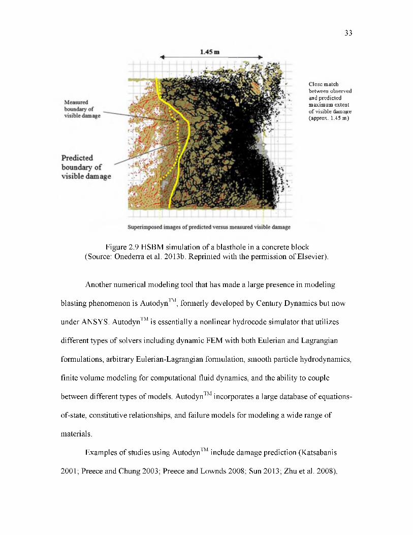
33

Close match between observed and predicted maximum extent o f visible damage (approx. 1.45 m)

Figure 2.9 HSBM simulation of a blasthole in a concrete block(Source: Onederra et al. 2013b. Reprinted with the permission of Elsevier).

Another numerical modeling tool that has made a large presence in modeling

blasting phenomenon is Autodyn™, formerly developed by Century Dynamics but now

under ANSYS. Autodyn™ is essentially a nonlinear hydrocode simulator that utilizes

different types of solvers including dynamic FEM with both Eulerian and Lagrangian

formulations, arbitrary Eulerian-Lagrangian formulation, smooth particle hydrodynamics,

finite volume modeling for computational fluid dynamics, and the ability to couple

between different types of models. Autodyn™ incorporates a large database of equations-

of-state, constitutive relationships, and failure models for modeling a wide range of

materials.

Examples of studies using Autodyn™ include damage prediction (Katsabanis

2001; Preece and Chung 2003; Preece and Lownds 2008; Sun 2013; Zhu et al. 2008),

34

crack prediction (Banadaki 2010; Zhu et al. 2007), cratering (ISEE 2011), air decking

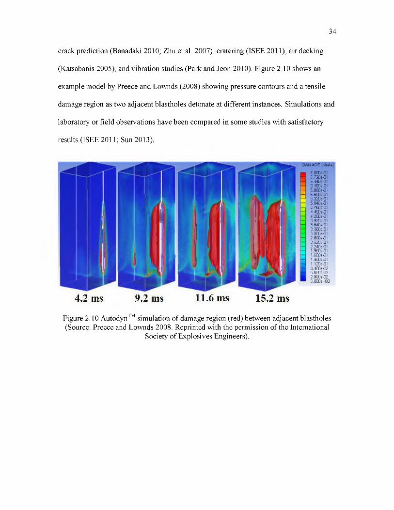
(Katsabanis 2005), and vibration studies (Park and Jeon 2010). Figure 2.10 shows an

example model by Preece and Lownds (2008) showing pressure contours and a tensile

damage region as two adjacent blastholes detonate at different instances. Simulations and

laboratory or field observations have been compared in some studies with satisfactory

results (ISEE 2011; Sun 2013).

rtAGE | shale|

70006-01 6720e-01 6.440e-01 6 160e-01 5 a80e-015.600e-01 5320e-01 5.0408-01 4 760e-014 4B0e-01 4.2006-01 3 920e-01 3.6406-01 3 360e-01 3 0806-01 2 .8006-01 2 520e-01 2240e-01 1 9606-011 680e-01 1.4006-01 1 1206-01 8400e-025 6006-022 800e-02 O.OOOe-KIO

4.2 ms 9.2 ms 11.6 ms 15.2 ms

Figure 2.10 AutodynTM simulation of damage region (red) between adjacent blastholes (Source: Preece and Lownds 2008. Reprinted with the permission of the International

Society of Explosives Engineers).

3. EXPERIMENTAL PROCEDURE

To obtain experimental data on near-field blast damage, a field test was conducted

at a surface mine located in Western Utah. A rhyolite outcrop was selected as the test site.

The top of the outcrop was level with the ground surface. A single, confined blasthole,

loaded with ammonium-nitrate fuel oil (ANFO) blasting agent detonated. Instrumentation

was positioned in nearby drillholes and on the surface to record the vibrations and

observe the blast damage. Observation of the drill and drilling rates for the blasthole and

monitoring holes indicated the test area was fairly uniform throughout the depth of the

test. The equipment, field experiment setup, and results are presented as follows.

3.1 Equipment summary

Three forms of instrumentation were chosen for measuring the effects of the

explosive charge in rock:

• Vibration transducers,

• Borescope, and

• Time-domain reflectometer (TDR).

Vibration transducers, clear acrylic tubing, and thin, two-conductor twisted wires

were grouted downhole using quick-setting Hydro-Stone® cement. The vibration

transducers were selected to record the ground motion. Data collection was accomplished

using two oscilloscopes. Additional seismographs were placed on the surface using bolts

drilled into to rock outcrops and bonded with epoxy. A borescope was used in

conjunction with clear acrylic tubing to view cracks that formed in the cement grout.

Thin two-conductor wires positioned downhole were analyzed with the TDR meter to

detect stretching or breaking.

3.1.1 Vibration transducers

Four uniaxial vibration transducers were selected for downhole vibration records.

In addition, 3 triaxial seismographs were secured on the surface. All of the transducers

were geophones, with the exception of one accelerometer.

3.1.1.1 Geophones

Geospace GS-20DM geophones were selected for use in obtaining near-field

vibration histories. Two different natural frequencies—28 Hz and 40 Hz—were picked so

a comparison between the two could be made. Both can operate at a 90° tilt angle and

remain within tolerance. The GS-20DM are designed to be 50% smaller than traditional

geophones and thus employ a smaller moving mass and stronger magnets (Geospace

Technologies 2012). It was anticipated that a smaller moving mass would allow the

geophone to withstand higher shock. Spurious frequencies can occur beyond 600 Hz for

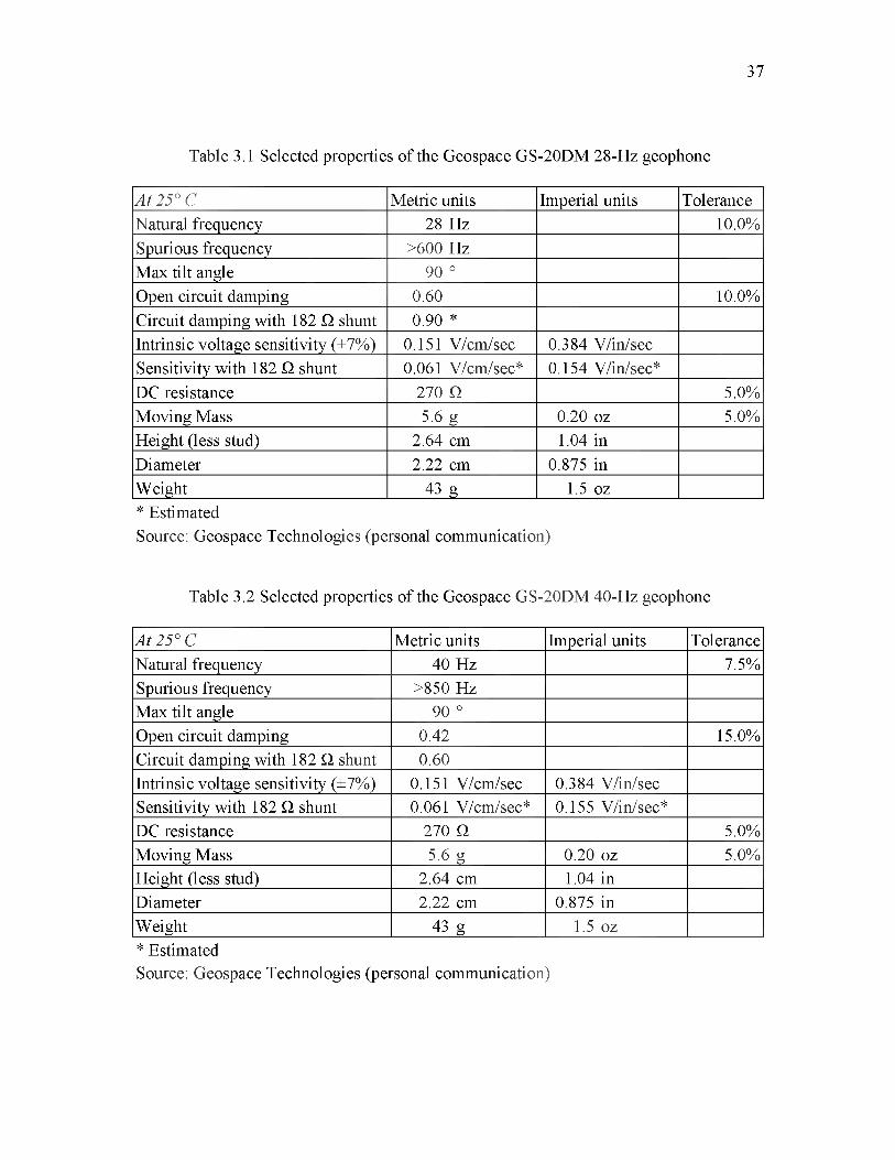
the 28-Hz geophone and 850 Hz for the 40-Hz geophone. Tables 3.1 and 3.2 list selected

properties for each of the geophones used. Figures 3.1 and 3.2 display the manufacturer’s

frequency response curves for each geophone with different shunt resistances applied.

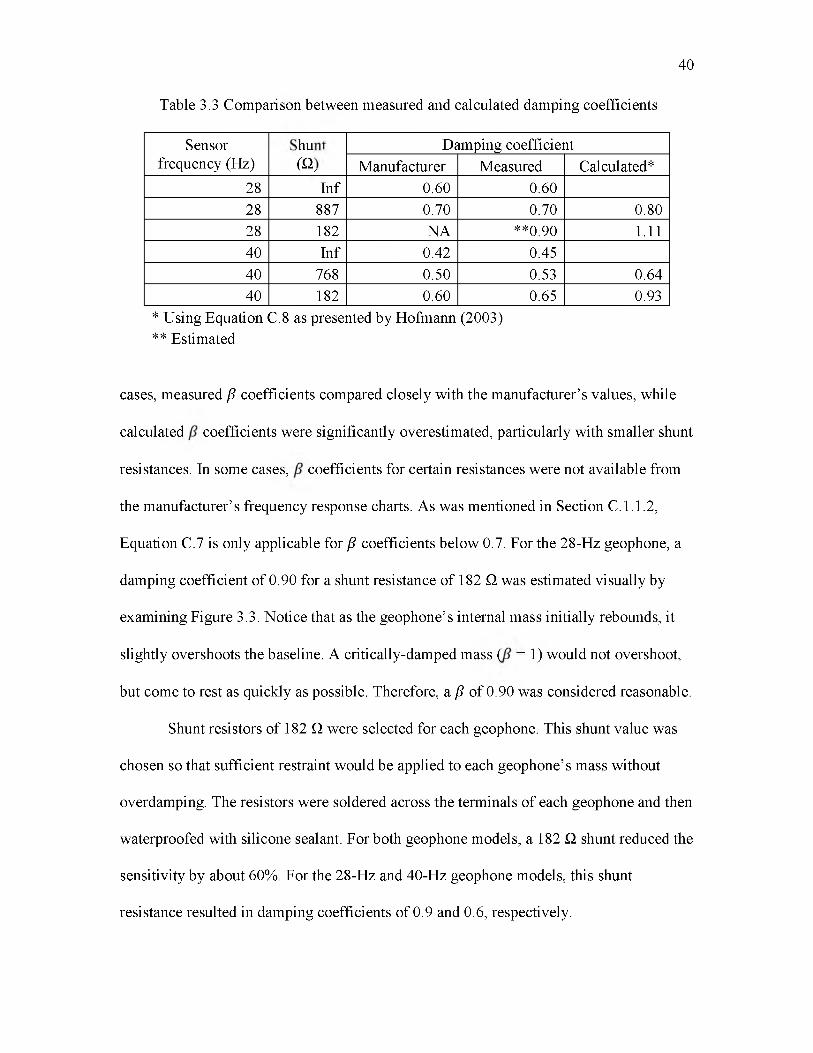
A comparison of the damping effects of different shunt resistors was conducted

on both geophone models. Using the procedure described in Section C.1.1.2 and Equation

C.7, damping coefficients (denoted as / ) were calculated and compared with the

manufacturer’s values and Equation C.8. The results are presented in Table 3.3. In most

36

37

Table 3.1 Selected properties of the Geospace GS-20DM 28-Hz geophone

At 25°C Metric units Imperial units ToleranceNatural frequency 28 Hz 10.0%Spurious frequency >600 HzMax tilt angle 90 °Open circuit damping 0.60 10.0%Circuit damping with 182 Q shunt 0.90 *Intrinsic voltage sensitivity (±7%) 0.151 V/cm/sec 0.384 V/in/secSensitivity with 182 Q shunt 0.061 V/cm/sec* 0.154 V/in/sec*DC resistance 270 Q 5.0%Moving Mass 5.6 g 0.20 oz 5.0%Height (less stud) 2.64 cm 1.04 inDiameter 2.22 cm 0.875 inWeight 43 g 1.5 oz* EstimatedSource: Geospace Technologies (personal communication)

Table 3.2 Selected properties of the Geospace GS-20DM 40-Hz geophone

At 25°C Metric units Imperial units ToleranceNatural frequency 40 Hz 7.5%Spurious frequency >850 HzMax tilt angle 90 °Open circuit damping 0.42 15.0%Circuit damping with 182 Q shunt 0.60Intrinsic voltage sensitivity (±7%) 0.151 V/cm/sec 0.384 V/in/secSensitivity with 182 Q shunt 0.061 V/cm/sec* 0.155 V/in/sec*DC resistance 270 Q 5.0%Moving Mass 5.6 g 0.20 oz 5.0%Height (less stud) 2.64 cm 1.04 inDiameter 2.22 cm 0.875 inWeight 43 g 1.5 oz* EstimatedSource: Geospace Technologies (personal communication)

Figure 3.1 Frequency response curve for GS-20DM geophone, 28-Hz model(Source: Geospace Technologies, personal communication. Reprinted with permission of Geospace Technologies).

38

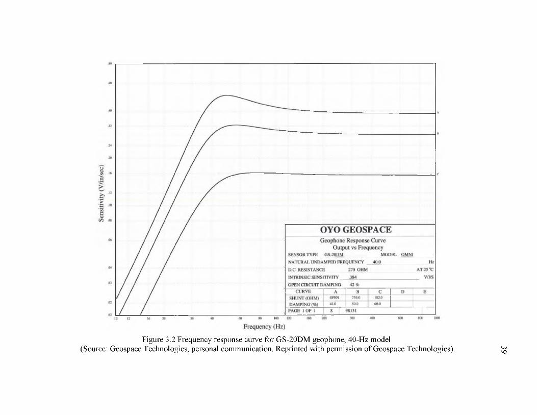
Figure 3.2 Frequency response curve for GS-20DM geophone, 40-Hz model(Source: Geospace Technologies, personal communication. Reprinted with permission of Geospace Technologies).

39

40

Table 3.3 Comparison between measured and calculated damping coefficients

Sensor frequency (Hz)

tnt )

£ £

S(

Damping coefficientManufacturer Measured Calculated*

28 Inf 0.60 0.6028 887 0.70 0.70 0.8028 182 NA **0.90 1.1140 Inf 0.42 0.4540 768 0.50 0.53 0.6440 182 0.60 0.65 0.93

* Using Equation C.8 as presented by Hofmann (2003) ** Estimated

cases, measured / coefficients compared closely with the manufacturer’s values, while

calculated coefficients were significantly overestimated, particularly with smaller shunt

resistances. In some cases, coefficients for certain resistances were not available from

the manufacturer’s frequency response charts. As was mentioned in Section C.1.1.2,

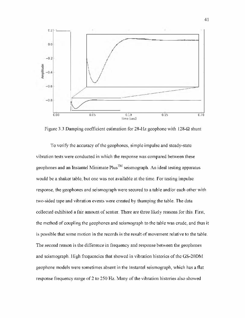
Equation C.7 is only applicable for / coefficients below 0.7. For the 28-Hz geophone, a

damping coefficient of 0.90 for a shunt resistance of 182 Q was estimated visually by

examining Figure 3.3. Notice that as the geophone’s internal mass initially rebounds, it

slightly overshoots the baseline. A critically-damped mass ( = 1) would not overshoot,

but come to rest as quickly as possible. Therefore, a / of 0.90 was considered reasonable.

Shunt resistors of 182 Q were selected for each geophone. This shunt value was

chosen so that sufficient restraint would be applied to each geophone’s mass without

overdamping. The resistors were soldered across the terminals of each geophone and then

waterproofed with silicone sealant. For both geophone models, a 182 Q shunt reduced the

sensitivity by about 60%. For the 28-Hz and 40-Hz geophone models, this shunt

resistance resulted in damping coefficients of 0.9 and 0.6, respectively.

41

0.2FT:

0.00 0.05 0.10 0 .15 0.20Time (sec)

Figure 3.3 Damping coefficient estimation for 28-Hz geophone with 128-Q shunt

To verify the accuracy of the geophones, simple impulse and steady-state

vibration tests were conducted in which the response was compared between these

geophones and an Instantel Minimate PlusTM seismograph. An ideal testing apparatus

would be a shaker table, but one was not available at the time. For testing impulse

response, the geophones and seismograph were secured to a table and/or each other with

two-sided tape and vibration events were created by thumping the table. The data

collected exhibited a fair amount of scatter. There are three likely reasons for this. First,

the method of coupling the geophones and seismograph to the table was crude, and thus it

is possible that some motion in the records is the result of movement relative to the table.

The second reason is the difference in frequency and response between the geophones

and seismograph. High frequencies that showed in vibration histories of the GS-20DM

geophone models were sometimes absent in the Instantel seismograph, which has a flat

response frequency range of 2 to 250 Hz. Many of the vibration histories also showed

different oscillation patterns after the initial impulse event, particularly between the

geophones and the seismograph, indicating that different oscillatory behaviors of the

internal masses were occurring. The third reason could be a difference in phase response.

The direction of each impulse event (up or down) was recorded. Tests showed that the

Instantel seismograph did not autocorrect for phase, and since its lowest flat response

frequency is 2 Hz, its measurements could appear dissimilar at frequencies below the

natural frequencies of the 28-Hz and 40-Hz geophones.

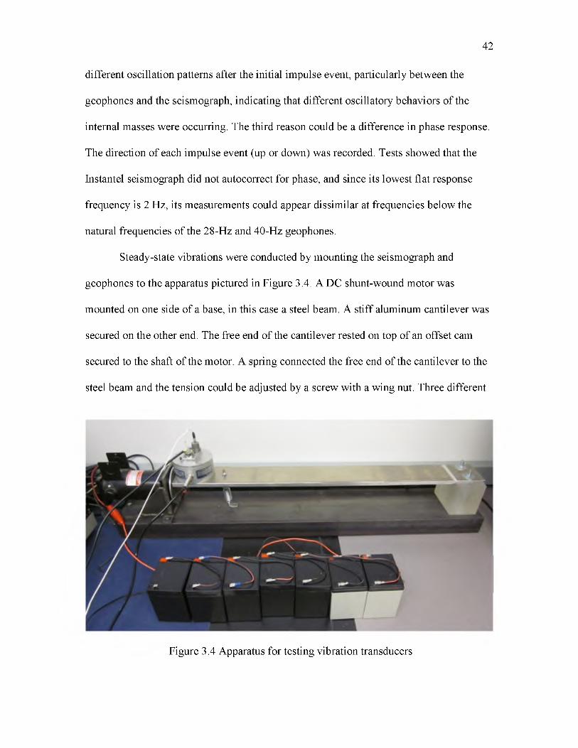
Steady-state vibrations were conducted by mounting the seismograph and

geophones to the apparatus pictured in Figure 3.4. A DC shunt-wound motor was

mounted on one side of a base, in this case a steel beam. A stiff aluminum cantilever was

secured on the other end. The free end of the cantilever rested on top of an offset cam

secured to the shaft of the motor. A spring connected the free end of the cantilever to the

steel beam and the tension could be adjusted by a screw with a wing nut. Three different

42

Figure 3.4 Apparatus for testing vibration transducers

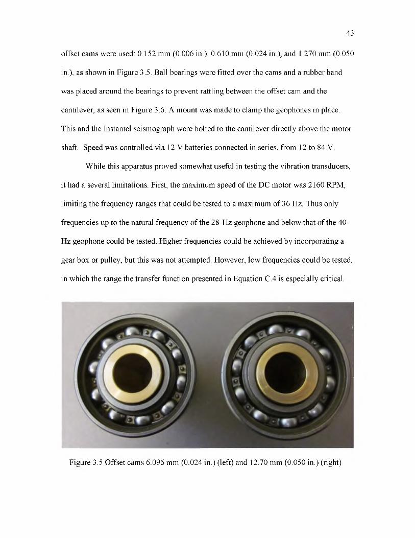
offset cams were used: 0.152 mm (0.006 in.), 0.610 mm (0.024 in.), and 1.270 mm (0.050

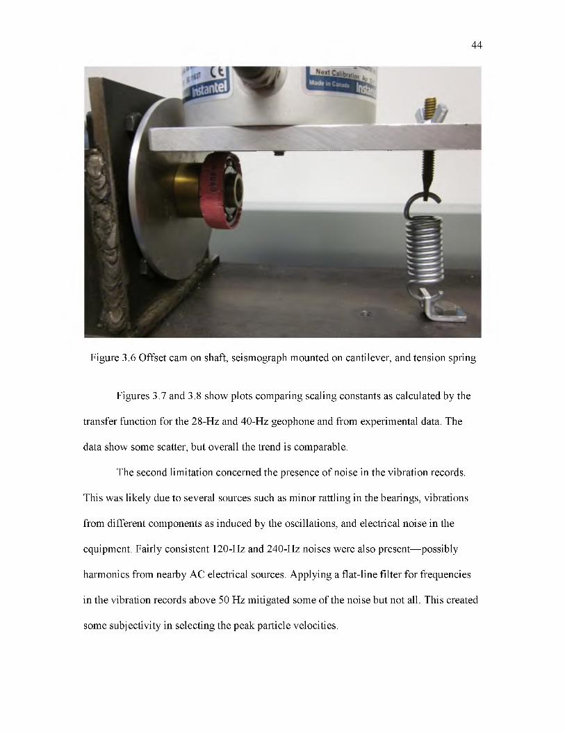
in.), as shown in Figure 3.5. Ball bearings were fitted over the cams and a rubber band

was placed around the bearings to prevent rattling between the offset cam and the

cantilever, as seen in Figure 3.6. A mount was made to clamp the geophones in place.

This and the Instantel seismograph were bolted to the cantilever directly above the motor

shaft. Speed was controlled via 12 V batteries connected in series, from 12 to 84 V.

While this apparatus proved somewhat useful in testing the vibration transducers,

it had a several limitations. First, the maximum speed of the DC motor was 2160 RPM,

limiting the frequency ranges that could be tested to a maximum of 36 Hz. Thus only

frequencies up to the natural frequency of the 28-Hz geophone and below that of the 40-

Hz geophone could be tested. Higher frequencies could be achieved by incorporating a

gear box or pulley, but this was not attempted. However, low frequencies could be tested,

in which the range the transfer function presented in Equation C.4 is especially critical.

43

Figure 3.5 Offset cams 6.096 mm (0.024 in.) (left) and 12.70 mm (0.050 in.) (right)

44

Figure 3.6 Offset cam on shaft, seismograph mounted on cantilever, and tension spring

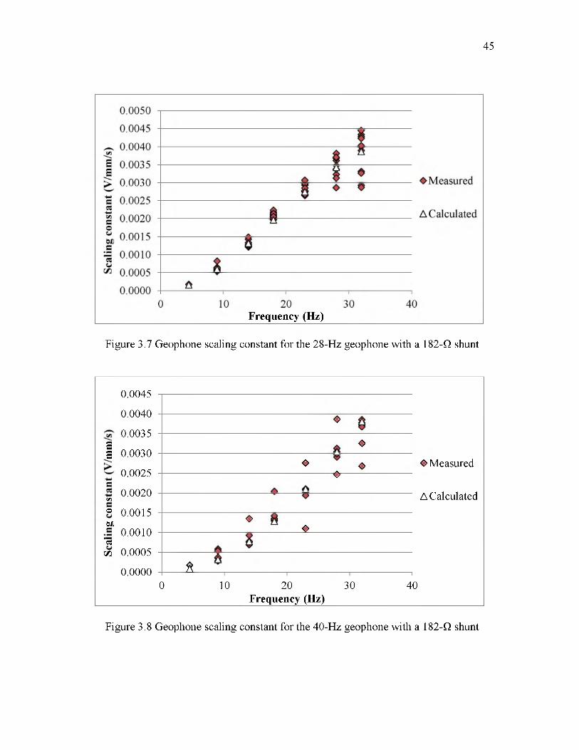
Figures 3.7 and 3.8 show plots comparing scaling constants as calculated by the

transfer function for the 28-Hz and 40-Hz geophone and from experimental data. The

data show some scatter, but overall the trend is comparable.

The second limitation concerned the presence of noise in the vibration records.

This was likely due to several sources such as minor rattling in the bearings, vibrations

from different components as induced by the oscillations, and electrical noise in the

equipment. Fairly consistent 120-Hz and 240-Hz noises were also present—possibly

harmonics from nearby AC electrical sources. Applying a flat-line filter for frequencies

in the vibration records above 50 Hz mitigated some of the noise but not all. This created

some subjectivity in selecting the peak particle velocities.

45

Frequency (Hz)

Figure 3.7 Geophone scaling constant for the 28-Hz geophone with a 182-Q shunt

EEEE

nVIn©cotj

"escin

0.0045

0.0040

0.0035

0.0030

0.0025

0.0020

0.0015

0.0010

0.0005

0.0000 *

♦♦

♦

♦

♦ ♦ o

10 20Frequency (Hz)

30

O Measured

A Calculated

--140

Figure 3.8 Geophone scaling constant for the 40-Hz geophone with a 182-Q shunt

0

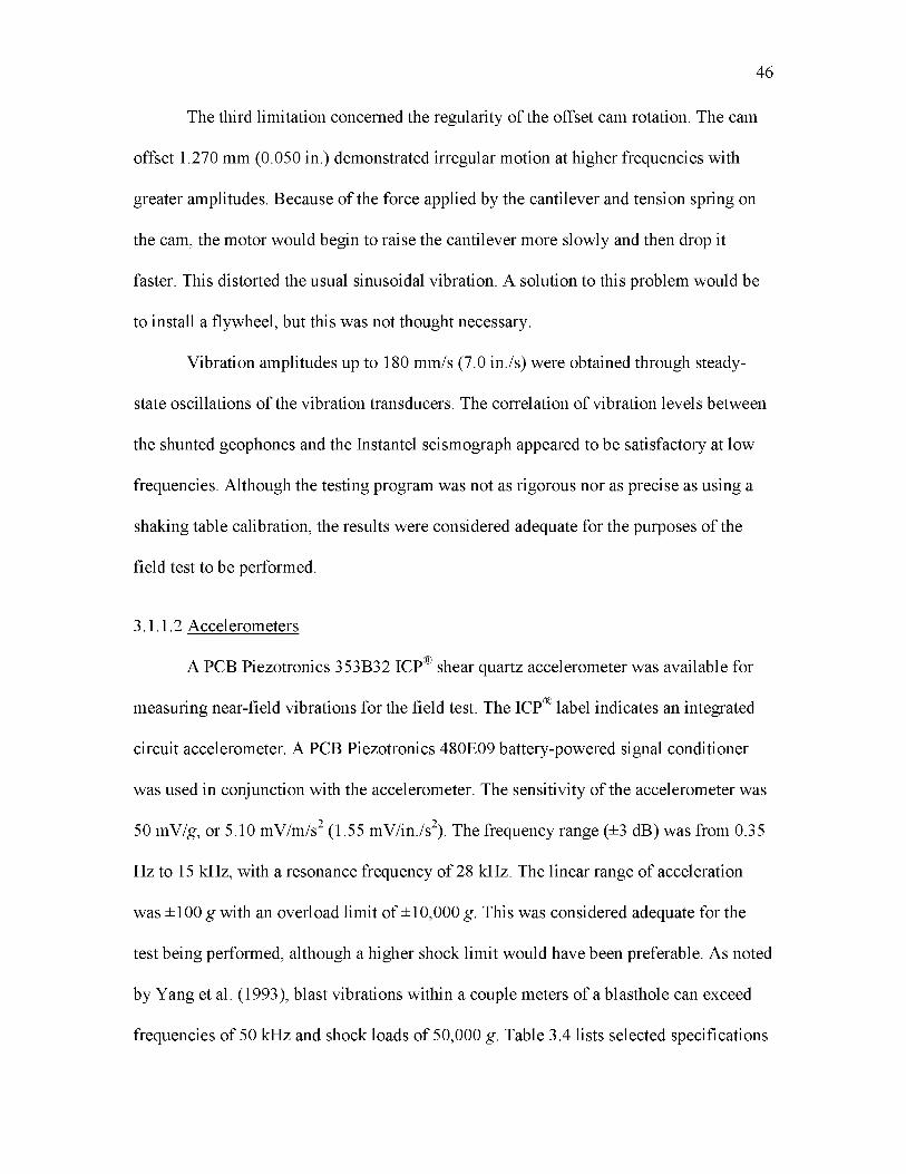
The third limitation concerned the regularity of the offset cam rotation. The cam

offset 1.270 mm (0.050 in.) demonstrated irregular motion at higher frequencies with

greater amplitudes. Because of the force applied by the cantilever and tension spring on

the cam, the motor would begin to raise the cantilever more slowly and then drop it

faster. This distorted the usual sinusoidal vibration. A solution to this problem would be

to install a flywheel, but this was not thought necessary.

Vibration amplitudes up to 180 mm/s (7.0 in./s) were obtained through steady-

state oscillations of the vibration transducers. The correlation of vibration levels between

the shunted geophones and the Instantel seismograph appeared to be satisfactory at low

frequencies. Although the testing program was not as rigorous nor as precise as using a

shaking table calibration, the results were considered adequate for the purposes of the

field test to be performed.

3.1.1.2 Accelerometers

A PCB Piezotronics 353B32 ICP® shear quartz accelerometer was available for

measuring near-field vibrations for the field test. The ICP® label indicates an integrated

circuit accelerometer. A PCB Piezotronics 480E09 battery-powered signal conditioner

was used in conjunction with the accelerometer. The sensitivity of the accelerometer was

50 mV/g, or 5.10 mV/m/s2 (1.55 mV/in./s2). The frequency range (±3 dB) was from 0.35

Hz to 15 kHz, with a resonance frequency of 28 kHz. The linear range of acceleration

was ±100 g with an overload limit of ±10,000 g. This was considered adequate for the

test being performed, although a higher shock limit would have been preferable. As noted

by Yang et al. (1993), blast vibrations within a couple meters of a blasthole can exceed

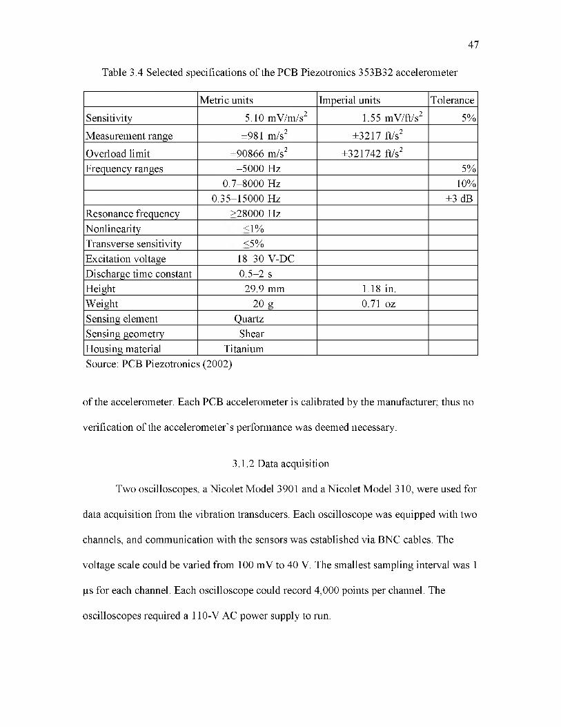
frequencies of 50 kHz and shock loads of 50,000 g. Table 3.4 lists selected specifications

46

47

Table 3.4 Selected specifications of the PCB Piezotronics 353B32 accelerometer

Metric units Imperial units Tolerance

Sensitivity 5.10 mV/m/s2 1.55 mV/ft/s2 5%

Measurement range ±981 m/s2 ±3217 ft/s2

Overload limit ±90866 m/s2 ±321742 ft/s2Frequency ranges -5000 Hz 5%

0.7-8000 Hz 10%0.35-15000 Hz ±3 dB

Resonance frequency >28000 HzNonlinearity <1%Transverse sensitivity <5%Excitation voltage 18-30 V-DCDischarge time constant 0.5-2 sHeight 29.9 mm 1.18 in.Weight 20 g 0.71 ozSensing element QuartzSensing geometry ShearHousing material TitaniumSource: PCB Piezotronics (2002)

of the accelerometer. Each PCB accelerometer is calibrated by the manufacturer; thus no

verification of the accelerometer’s performance was deemed necessary.

3.1.2 Data acquisition

Two oscilloscopes, a Nicolet Model 3901 and a Nicolet Model 310, were used for

data acquisition from the vibration transducers. Each oscilloscope was equipped with two

channels, and communication with the sensors was established via BNC cables. The

voltage scale could be varied from 100 mV to 40 V. The smallest sampling interval was 1

|is for each channel. Each oscilloscope could record 4,000 points per channel. The

oscilloscopes required a 110-V AC power supply to run.

Downloading data from the Nicolet 3901 required the use of a 25-pin crossover

serial cable and computer or laptop equipped with either a 25-pin serial port or a 9-pin

serial port and a 25-pin to 9-pin serial adapter. The download was accomplished using

Waveform Basic™ software. The Nicolet 310 possessed a dual-bay 3 '/2-in. floppy reader

that used double-density disks. Downloaded data entailed saving the data onto a disk and

using an executable program on a computer to extract each record.

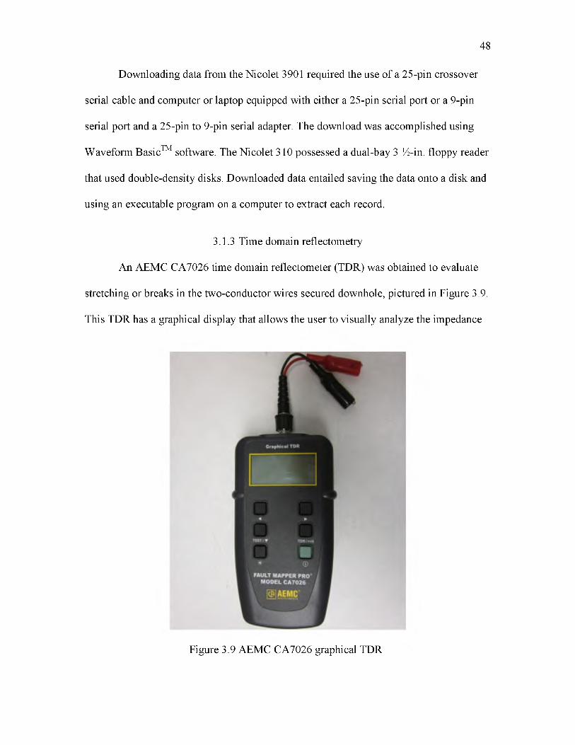
3.1.3 Time domain reflectometry

An AEMC CA7026 time domain reflectometer (TDR) was obtained to evaluate

stretching or breaks in the two-conductor wires secured downhole, pictured in Figure 3.9.

This TDR has a graphical display that allows the user to visually analyze the impedance

48

Figure 3.9 AEMC CA7026 graphical TDR

profile of the wire. Cable attachment could be made by either a BNC connector or

alligator clips. The resolution of the instrument, however, is limited. The graphical

display did not possess a zoom feature and thus measurements made by the cursor could

only be made within ±2-3 ft. Another limitation of the instrument was the occurrence of

an initial pulse at the beginning of the impedance profile. This effectively limited the

closest obtainable reading to at least 15 m (50 ft). An extra length of wire was required to

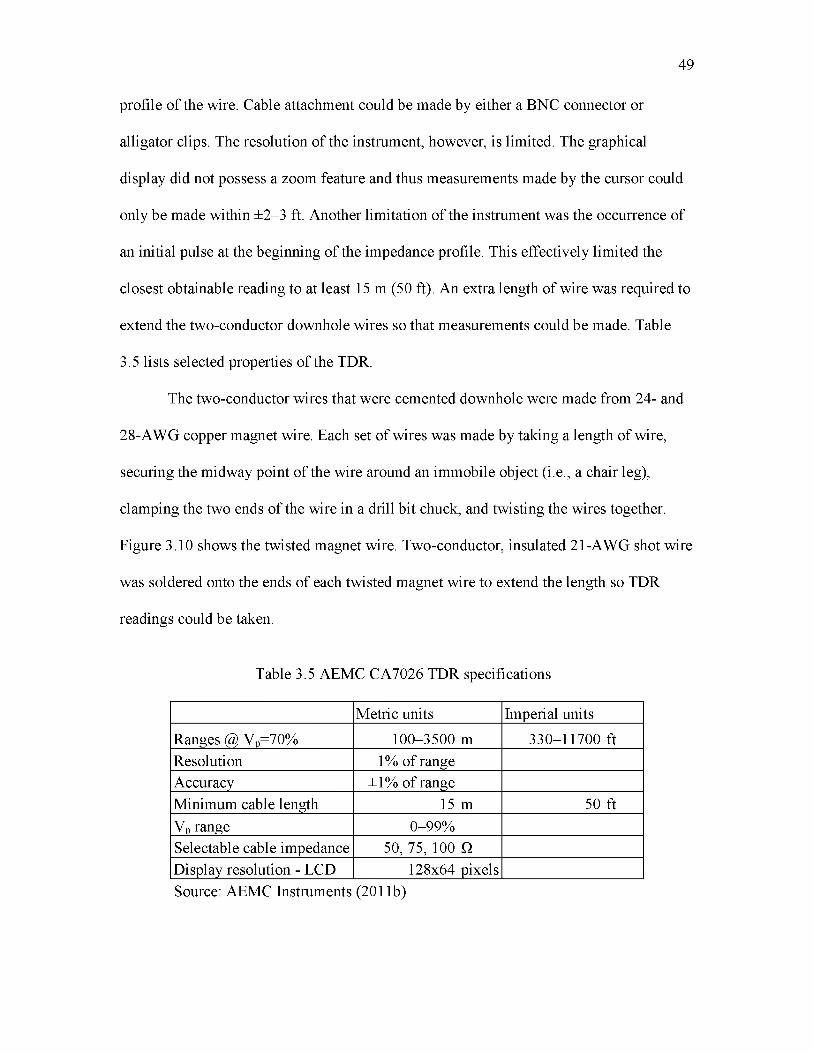
extend the two-conductor downhole wires so that measurements could be made. Table

3.5 lists selected properties of the TDR.

The two-conductor wires that were cemented downhole were made from 24- and

28-AWG copper magnet wire. Each set of wires was made by taking a length of wire,

securing the midway point of the wire around an immobile object (i.e., a chair leg),

clamping the two ends of the wire in a drill bit chuck, and twisting the wires together.

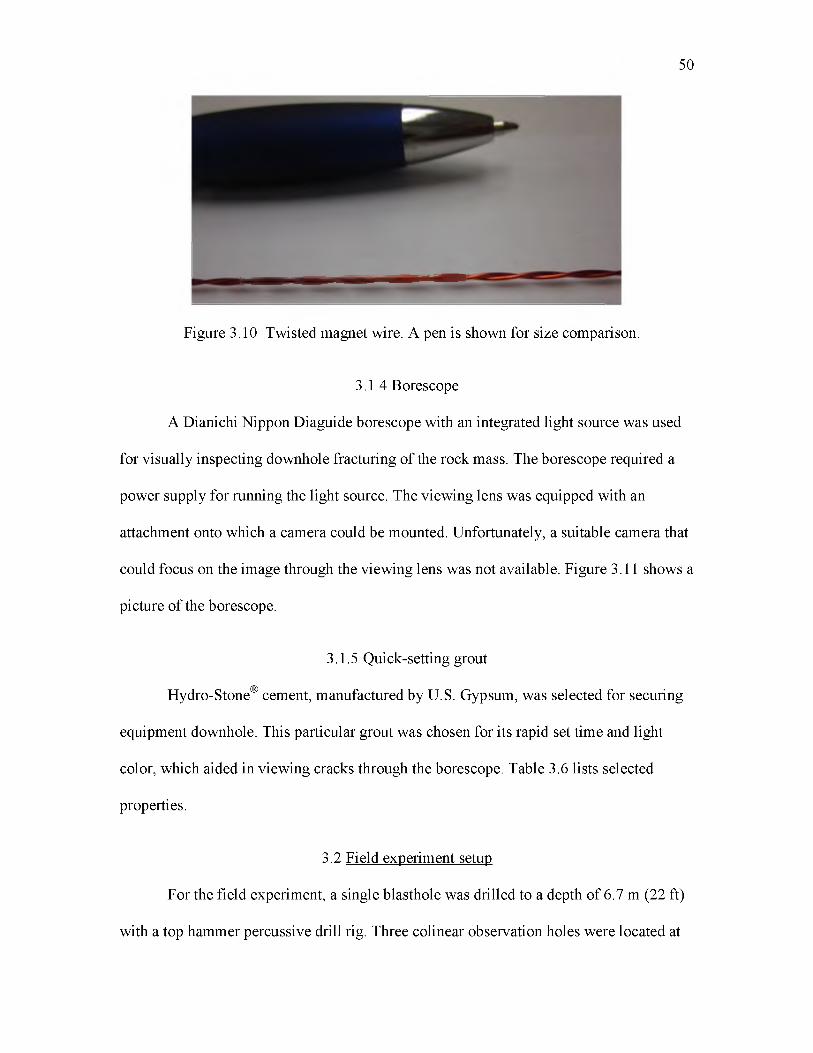
Figure 3.10 shows the twisted magnet wire. Two-conductor, insulated 21-AWG shot wire

was soldered onto the ends of each twisted magnet wire to extend the length so TDR

readings could be taken.

49

Table 3.5 AEMC CA7026 TDR specifications

Metric units Imperial units

Ranges @ Vp=70% 100-3500 m 330-11700 ftResolution 1% of rangeAccuracy ±1% of rangeMinimum cable length 15 m 50 ftVp range 0-99%Selectable cable impedance 50, 75, 100 QDisplay resolution - LCD 128x64 pixelsSource: AEMC Instruments (2011b)

50

Figure 3.10 Twisted magnet wire. A pen is shown for size comparison.

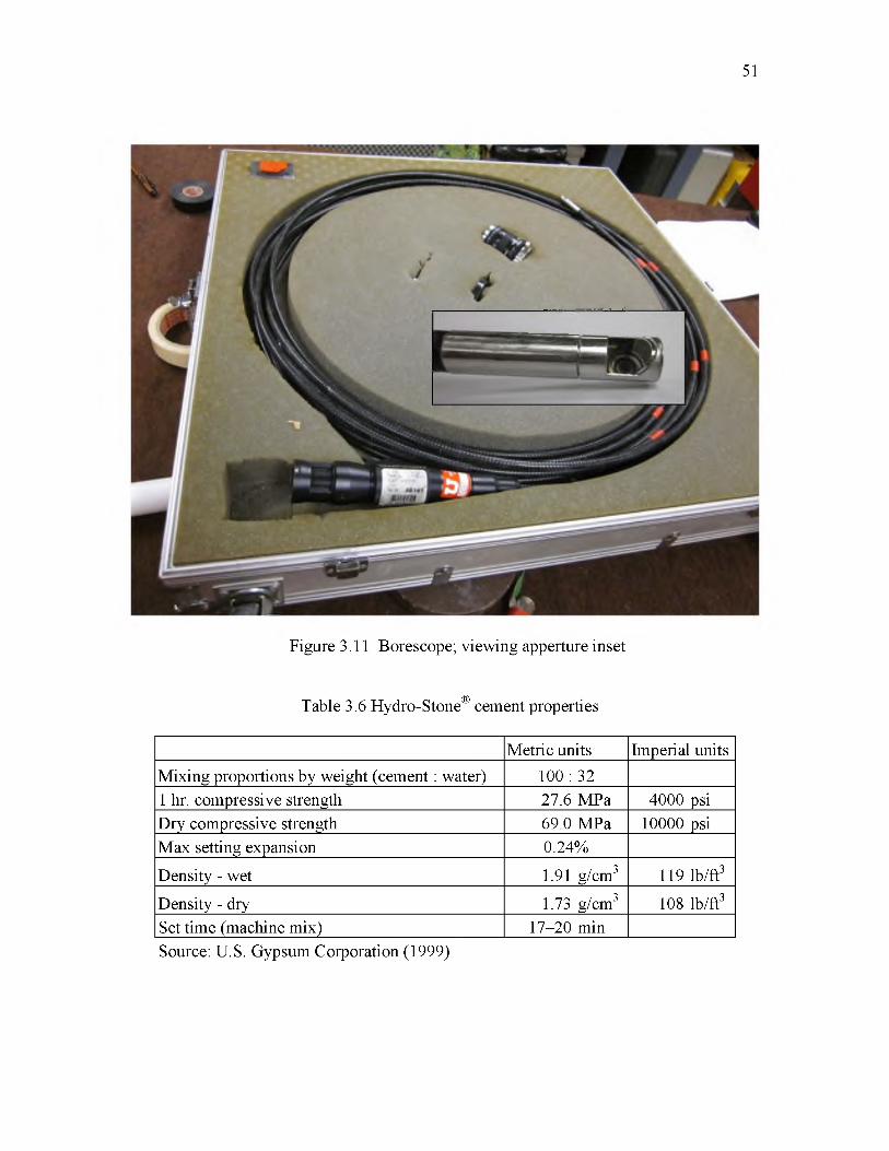
3.1.4 Borescope

A Dianichi Nippon Diaguide borescope with an integrated light source was used

for visually inspecting downhole fracturing of the rock mass. The borescope required a

power supply for running the light source. The viewing lens was equipped with an

attachment onto which a camera could be mounted. Unfortunately, a suitable camera that

could focus on the image through the viewing lens was not available. Figure 3.11 shows a

picture of the borescope.

3.1.5 Quick-setting grout

Hydro-Stone® cement, manufactured by U.S. Gypsum, was selected for securing

equipment downhole. This particular grout was chosen for its rapid set time and light

color, which aided in viewing cracks through the borescope. Table 3.6 lists selected

properties.

3.2 Field experiment setup

For the field experiment, a single blasthole was drilled to a depth of 6.7 m (22 ft)

with a top hammer percussive drill rig. Three colinear observation holes were located at

51

Figure 3.11 Borescope; viewing apperture inset

Table 3.6 Hydro-Stone® cement properties

Metric units Imperial unitsMixing proportions by weight (cement : water) 100 : 321 hr. compressive strength 27.6 MPa 4000 psiDry compressive strength 69.0 MPa 10000 psiMax setting expansion 0.24%

Density - wet 1.91 g/cm3 119 lb/ft3

Density - dry 1.73 g/cm3 108 lb/ft3Set time (machine mix) 17-20 minSource: U.S. Gypsum Corporation (1999)

distances of 1.1 m (3.5 ft), 2.1 m (6.9 ft), and 3.8 m (12.4 ft) to the south of the blasthole.

Each was drilled to a depth of 4.9 m (16 ft). The bit diameter used to drill the holes was

114.3 mm (4.5 in.); thus, a drillhole diameter of 120.7 mm (4.75 in.) was assumed. The

accelerometer and three shunted geophones were positioned down the two observation

holes furthest from the blasthole. Two Instantel DS-200 seismographs were positioned in

between the observation holes on the surface. An Instantel Minimate Plus seismograph

was positioned beyond the third observation hole. Diagrams of the setup are shown in

Figures 3.12 and 3.13. Table 3.7 gives a list of the vibration transducers in the diagrams.

To aid in securing the vibration transducers downhole, the accelerometer and

geophones were precast in Hydo-StoneTM as shown in Figure 3.14. A short length of PVC

pipe was placed in the top of the cast. Cardboard molds and wires were used to secure the

instruments, but during the casting process two of the geohones shifted positions slightly.

The amount of shifting was determined to be inconsequential. To position the instrument

casts downhole, additional lengths of PVC pipe were coupled to each cast. Each cast was

lowered downhole so that the axes of the vibration sensors were aligned in the direction

of the blasthole.

Two pairs of the two-conductor twisted wires for TDR measurements were

placed down each instrument hole. Each hole had one TDR wire configuration with 28-

AWG and one with 24-AWG magnet wire so a comparison could be made. Each TDR

wire configuration consisted of a 5.5-m (18-ft) length of twisted magnet wire downhole,

which was soldered to an 18.3-m (60-ft) length of shot wire. The only exception was the

length of 28-AWG wire down instrument hole 1. The wire was accidentally broken in

52

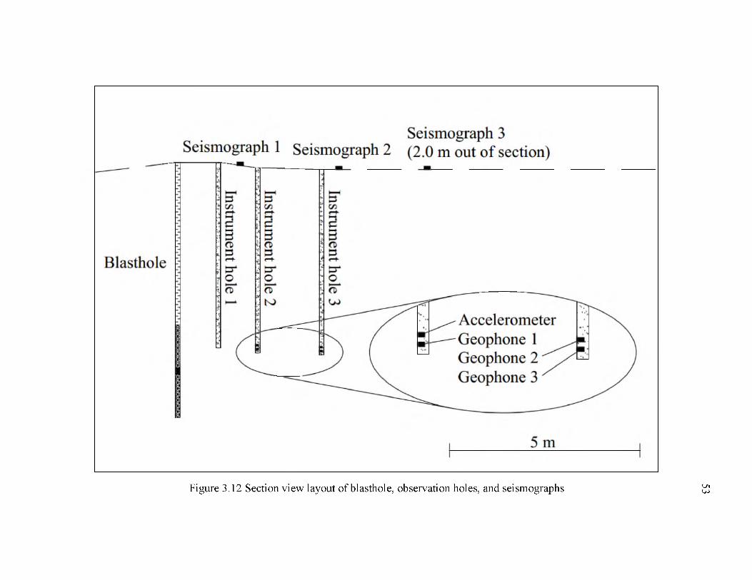
Figure 3.12 Section view layout of blasthole, observation holes, and seismographs

53

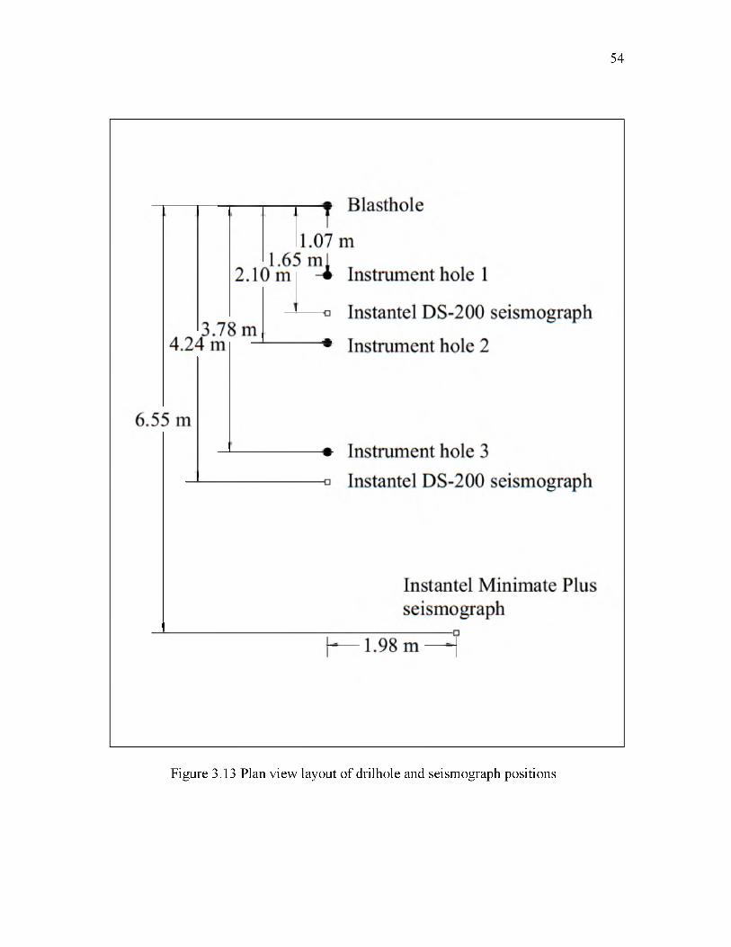
54

Figure 3.13 Plan view layout o f drilhole and seismograph positions

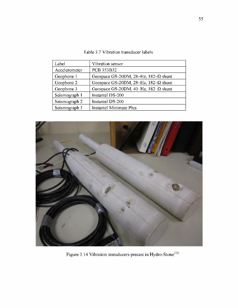
55

Table 3.7 Vibration transducer labels

Label Vibration sensorAccelerometer PCB 353B32Geophone 1 Geospace GS-20DM, 28-Hz, 182-Q shuntGeophone 2 Geospace GS-20DM, 28-Hz, 182-Q shuntGeophone 3 Geospace GS-20DM, 40-Hz, 182-Q shuntSeismograph 1 Instantel DS-200Seismograph 2 Instantel DS-200Seismograph 3 Instantel Minimate Plus

Figure 3.14 Vibration transducers precast in Hydro-Stone™

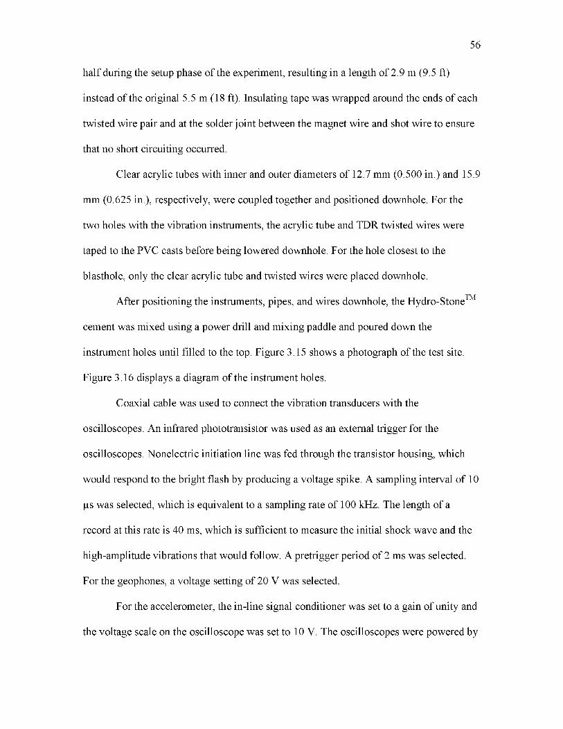
half during the setup phase of the experiment, resulting in a length of 2.9 m (9.5 ft)

instead of the original 5.5 m (18 ft). Insulating tape was wrapped around the ends of each

twisted wire pair and at the solder joint between the magnet wire and shot wire to ensure

that no short circuiting occurred.

Clear acrylic tubes with inner and outer diameters of 12.7 mm (0.500 in.) and 15.9

mm (0.625 in.), respectively, were coupled together and positioned downhole. For the

two holes with the vibration instruments, the acrylic tube and TDR twisted wires were

taped to the PVC casts before being lowered downhole. For the hole closest to the

blasthole, only the clear acrylic tube and twisted wires were placed downhole.

After positioning the instruments, pipes, and wires downhole, the Hydro-StoneTM

cement was mixed using a power drill and mixing paddle and poured down the

instrument holes until filled to the top. Figure 3.15 shows a photograph of the test site.

Figure 3.16 displays a diagram of the instrument holes.

Coaxial cable was used to connect the vibration transducers with the

oscilloscopes. An infrared phototransistor was used as an external trigger for the

oscilloscopes. Nonelectric initiation line was fed through the transistor housing, which

would respond to the bright flash by producing a voltage spike. A sampling interval of 10

|is was selected, which is equivalent to a sampling rate of 100 kHz. The length of a

record at this rate is 40 ms, which is sufficient to measure the initial shock wave and the

high-amplitude vibrations that would follow. A pretrigger period of 2 ms was selected.

For the geophones, a voltage setting of 20 V was selected.

For the accelerometer, the in-line signal conditioner was set to a gain of unity and

the voltage scale on the oscilloscope was set to 10 V. The oscilloscopes were powered by

56

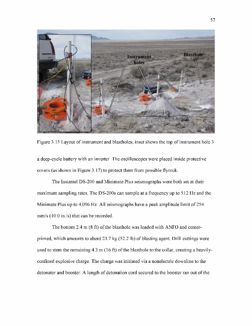
57

Figure 3.15 Layout of instrument and blastholes; inset shows the top of instrument hole 3.

a deep-cycle battery with an inverter. The oscilloscopes were placed inside protective

covers (as shown in Figure 3.17) to protect them from possible flyrock.

The Instantel DS-200 and Minimate Plus seismographs were both set at their

maximum sampling rates. The DS-200s can sample at a frequency up to 512 Hz and the

Minimate Plus up to 4,096 Hz. All seismographs have a peak amplitude limit of 254

mm/s (10.0 in./s) that can be recorded.

The bottom 2.4 m (8 ft) of the blasthole was loaded with ANFO and center-

primed, which amounts to about 23.7 kg (52.2 lb) of blasting agent. Drill cuttings were

used to stem the remaining 4.3 m (16 ft) of the blasthole to the collar, creating a heavily-

confined explosive charge. The charge was initiated via a nonelectric downline to the

detonator and booster. A length of detonation cord secured to the booster ran out of the

58

Figure 3.16 Section view layout of the blasthole and instrumented holes

59

Figure 3.17 Oscilliscopes in their protective covers, powered by a deep-cycle battery

hole collar and joined with another length of nonelectric initiation tube, which was

connected to the external trigger for the oscilloscopes.

3.3 Results

3.3.1 Vibration records

The raw vibration records are shown in Figures 3.18, 3.19, 3.20, and 3.21. The

20-V scale on the oscilloscope proved adequate for the geophones. However, the 10-V

scale, which is equivalent to 200 g of acceleration, was too low for the accelerometer.

The initial pressure peak and a secondary peak were clipped as the acceleration limit was

exceeded. Extrapolation of these first two peaks was performed, as is shown in Figure

3.22. The estimated shock experienced by the accelerometer is at least 450 g. This is

lower than the near-field accelerations expected by Yang et al. (1993). Since the linear

acceleration range of this particular accelerometer was exceeded (±200 g), the

extrapolation is only a rough estimate.

10

5

>Of

000 001 002 003 004Time (s)

Figure 3.18 Accelerometer record (raw)

60

OOO 001 002 003 004Time (s)

Figure 3.19 Geophone 1 record (raw)

61

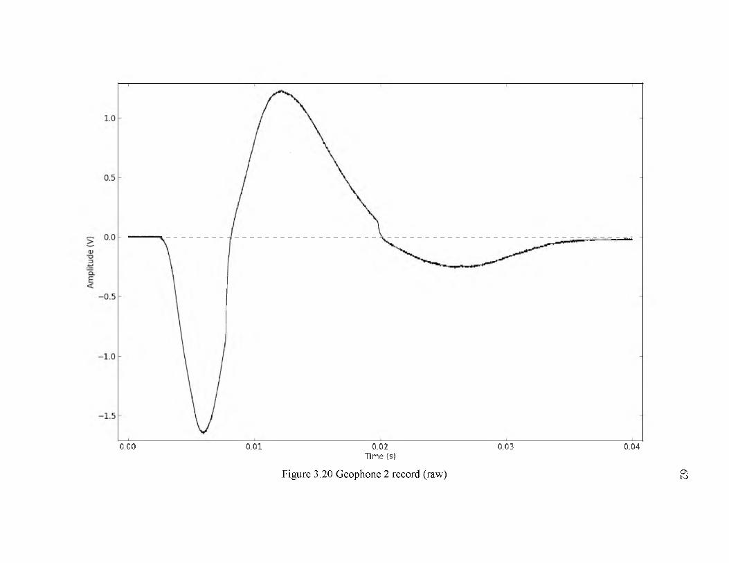
0.00 0.01 0.02 0.03 0.04Time (s)

Figure 3.20 Geophone 2 record (raw)

62

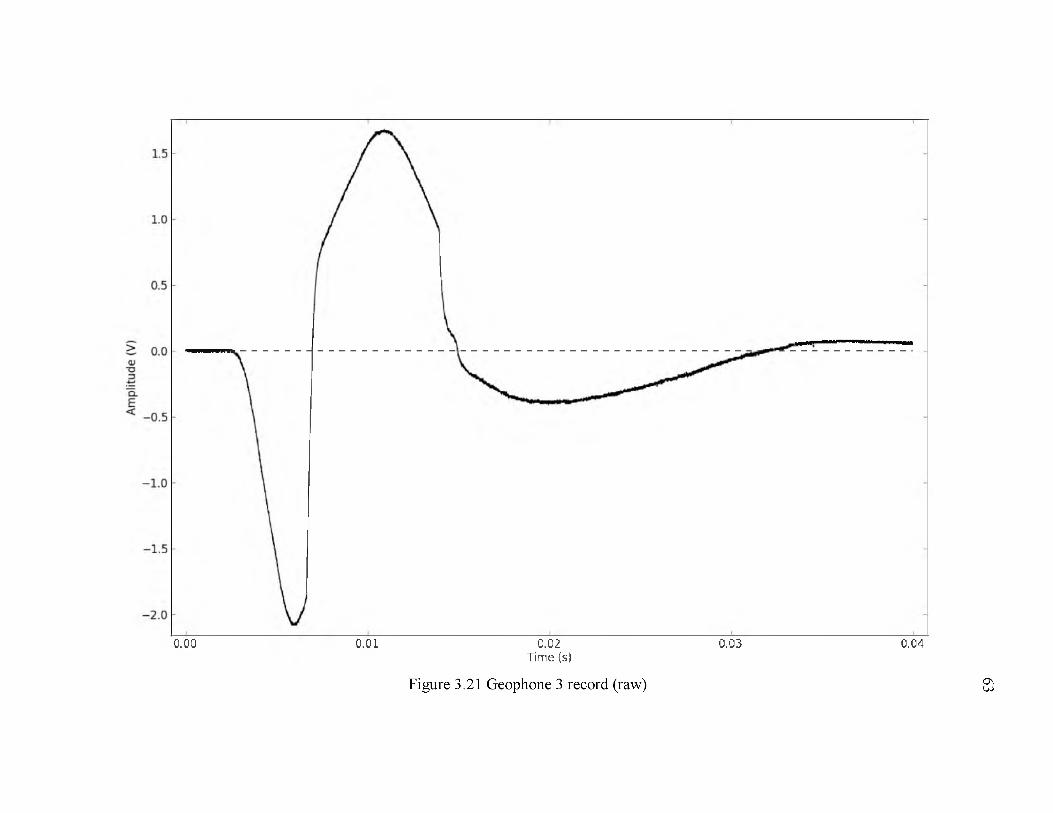
0.00 0.01 0.02 0.03 0.04Time (s)

Figure 3.21 Geophone 3 record (raw)

63

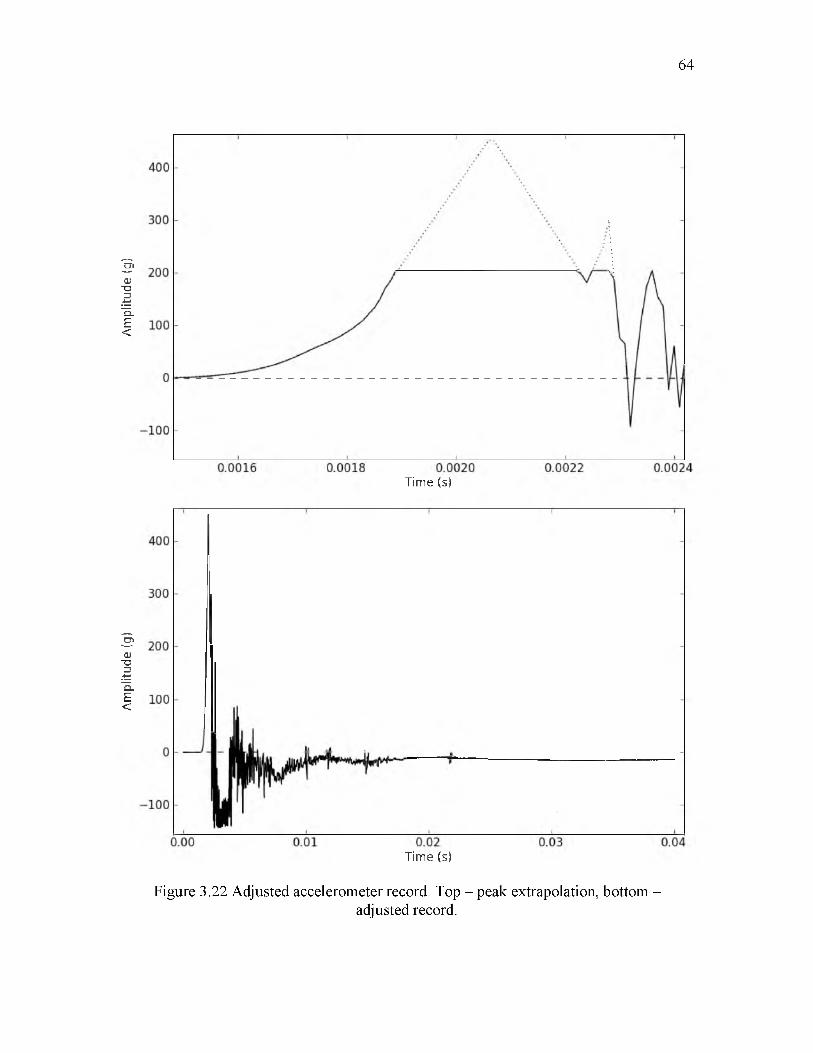
Ampl

itude

(g

) Am

plitu

de

(g)

64

Time (s)

Time (s)

Figure 3.22 Adjusted accelerometer record. Top - peak extrapolation, bottom -adjusted record.

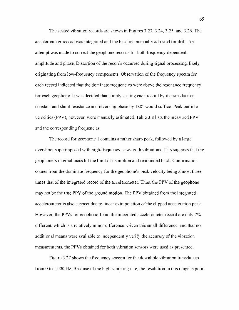
The scaled vibration records are shown in Figures 3.23, 3.24, 3.25, and 3.26. The

accelerometer record was integrated and the baseline manually adjusted for drift. An

attempt was made to correct the geophone records for both frequency-dependent

amplitude and phase. Distortion of the records occurred during signal processing, likely

originating from low-frequency components. Observation of the frequency spectra for

each record indicated that the dominate frequencies were above the resonance frequency

for each geophone. It was decided that simply scaling each record by its transduction

constant and shunt resistance and reversing phase by 180° would suffice. Peak particle

velocities (PPV), however, were manually estimated. Table 3.8 lists the measured PPV

and the corresponding frequencies.

The record for geophone 1 contains a rather sharp peak, followed by a large

overshoot superimposed with high-frequency, saw-tooth vibrations. This suggests that the

geophone’s internal mass hit the limit of its motion and rebounded back. Confirmation

comes from the dominate frequency for the geophone’s peak velocity being almost three

times that of the integrated record of the accelerometer. Thus, the PPV of the geophone

may not be the true PPV of the ground motion. The PPV obtained from the integrated

accelerometer is also suspect due to linear extrapolation of the clipped acceleration peak.

However, the PPVs for geophone 1 and the integrated accelerometer record are only 7%

different, which is a relatively minor difference. Given this small difference, and that no

additional means were available to independently verify the accurary of the vibration

measurements, the PPVs obtained for both vibration sensors were used as presented.

Figure 3.27 shows the frequency spectra for the downhole vibration transducers

from 0 to 1,000 Hz. Because of the high sampling rate, the resolution in this range is poor

65

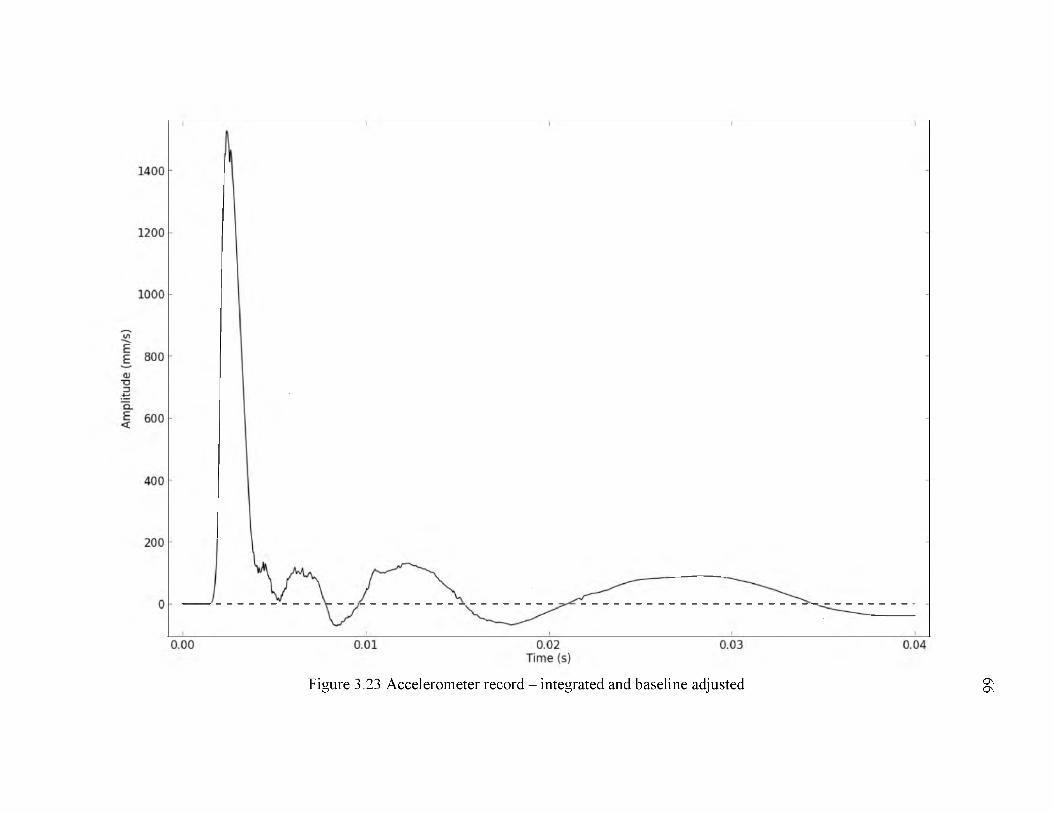
Figure 3.23 Accelerometer record - integrated and baseline adjusted

66

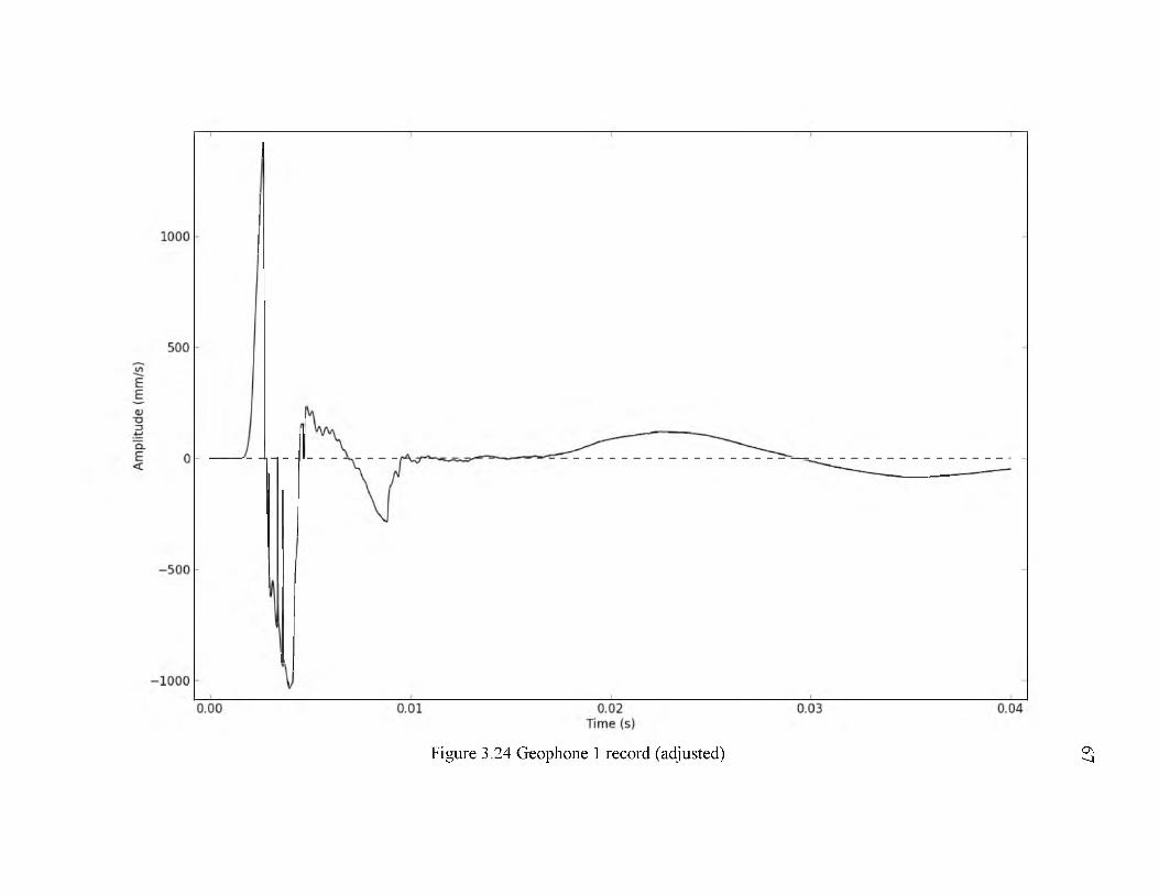
Figure 3.24 Geophone 1 record (adjusted)

67

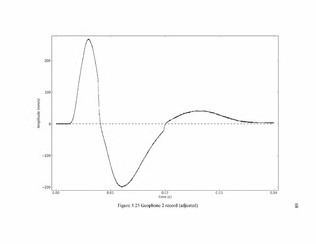
0.00 0.01 0.02 0.03 0.04Time (s)

Figure 3.25 Geophone 2 record (adjusted)

68

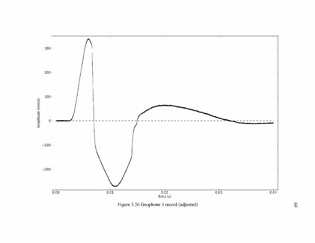
0.00 0.01 0.02 0.03 0.04Time (s)

Figure 3.26 Geophone 3 record (adjusted)

69

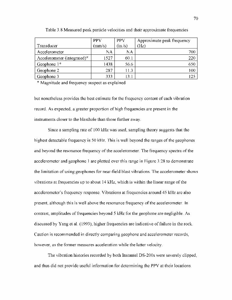
70

Table 3.8 Measured peak particle velocities and their approximate frequencies

TransducerPPV(mm/s)

PPV(in./s)

Approximate peak frequency (Hz)

Accelerometer NA NA 700Accelerometer (integrated)* 1527 60.1 220Geophone 1* 1438 56.6 650Geophone 2 287 11.3 100Geophone 3 333 13.1 125* Magnitude and frequency suspect as explained

but nonetheless provides the best estimate for the frequency content of each vibration

record. As expected, a greater proportion of high frequencies are present in the

instruments closer to the blasthole than those farther away.

Since a sampling rate of 100 kHz was used, sampling theory suggests that the

highest detectable frequency is 50 kHz. This is well beyond the ranges of the geophones

and beyond the resonance frequency of the accelerometer. The frequency spectra of the

accelerometer and geophone 1 are plotted over this range in Figure 3.28 to demonstrate

the limitation of using geophones for near-field blast vibrations. The accelerometer shows

vibrations at frequencies up to about 14 kHz, which is within the linear range of the

accelerometer’s frequency response. Vibrations at frequencies around 45 kHz are also

present, although this is well above the resonance frequency of the accelerometer. In

contrast, amplitudes of frequencies beyond 5 kHz for the geophone are negligible. As

discussed by Yang et al. (1993), higher frequencies are indicative of failure in the rock.

Caution is recommended in directly comparing geophone and accelerometer records,

however, as the former measures acceleration while the latter velocity.

The vibration histories recorded by both Instantel DS-200s were severely clipped,

and thus did not provide useful information for determining the PPV at their locations.

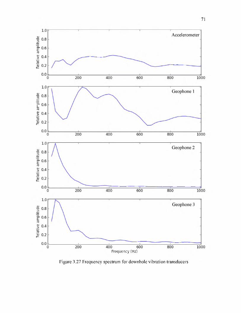
Rela

tive

ampl

itude

Re

lativ

e am

plitu

de

Rela

tive

ampl

itude

Re

lativ

e am

plit

ude

71

Frequency (Hz)

Figure 3.27 Frequency spectrum for downhole vibration transducers

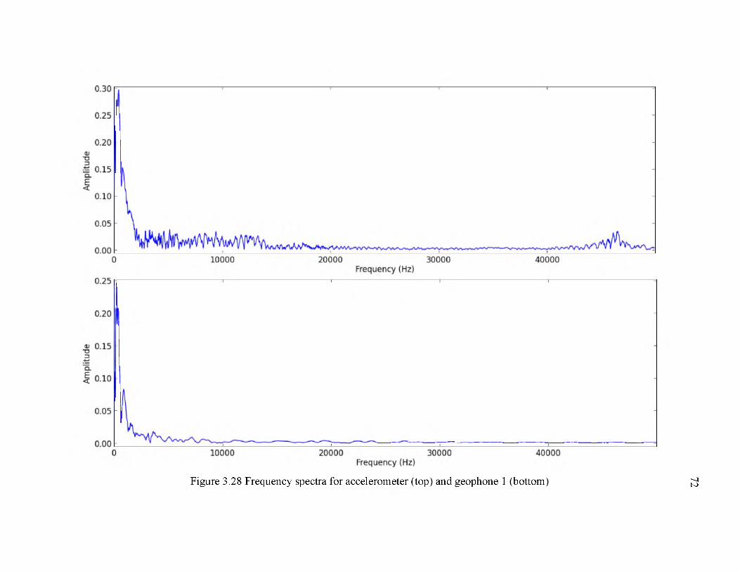
Figure 3.28 Frequency spectra for accelerometer (top) and geophone 1 (bottom)

72

The vibration history recorded by the Instantel Minimate Plus barely clipped on the

longitudinal axis of motion, and thus the PPV at its location was measured to be 254

mm/s (10.0 in./s). For completeness, the initial portions of the vibration records for all

three seismographs are displayed below in Figures 3.29, 3.30, and 3.31.

3.3.2 TDR results

TDR measurements of the downhole twisted wire pairs were able to detect

movement of the rock around the blasthole. The thinner 28-AWG magnet wire proved to

be more sensitive and was considered more useful than the 24-AWG wire. Because of the

poor resolution of the TDR, it was difficult to ascertain the exact depth for each event

detected. The best that could be determined was whether the damage occurred in the top,

middle, or bottom third of the blasthole. Only one wire, the 28-AWG wire in instrument

hole 1 closest to the blast, sheared completely near the top of the hole. The 24-AWG wire

in the same hole appeared stretched along the length of the hole, indicating damage along

the entire length of the hole. In instrument hole 2, the 28-AWG wire detected shifting of

the rock in the top and middle sections of the blasthole. The 24-AWG wire in the same

hole did not change. In instrument hole 3, virtually no permanent rock displacement was

measured. Table 3.9 lists the TDR-measured lengths of each wire before and after the

blast using a Vp value of 73%. Figure 3.32 shows digitized versions of the impedance

signals measured with the TDR. The precision of the TDR readings obtained by the

screen cursor with the stated Vp was ±0.9 m (3 ft).

73

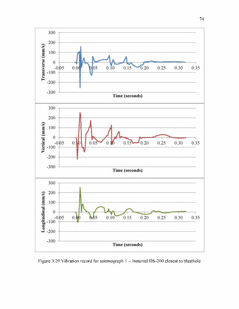
74

Figure 3.29 Vibration record for seismograph 1 - Instantel DS-200 closest to blasthole

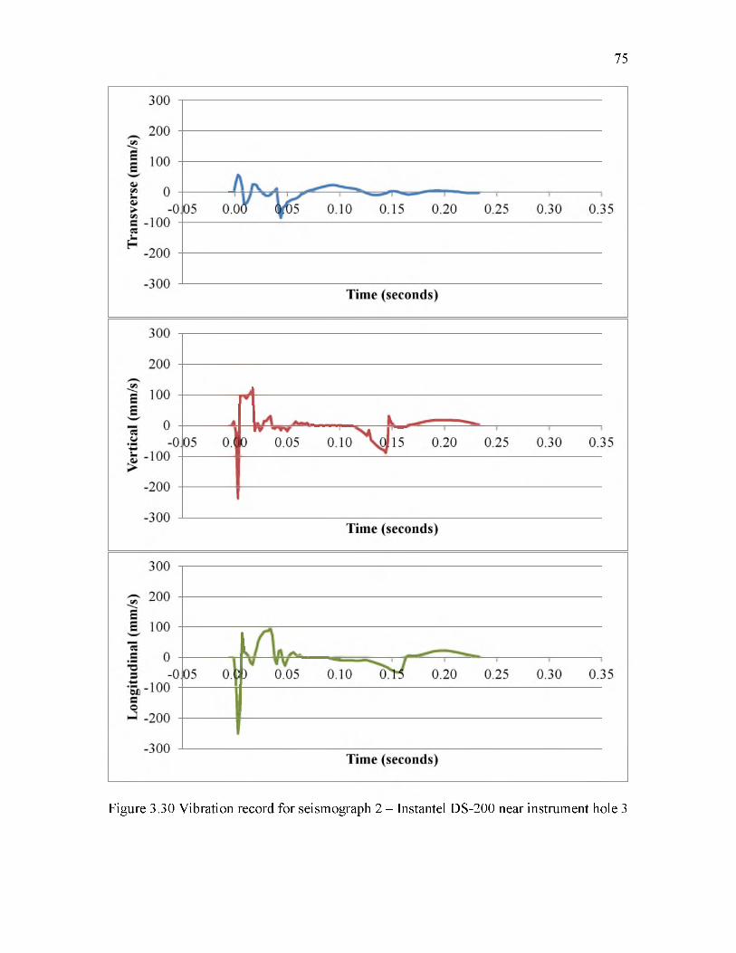
75

Figure 3.30 Vibration record for seismograph 2 - Instantel DS-200 near instrument hole 3

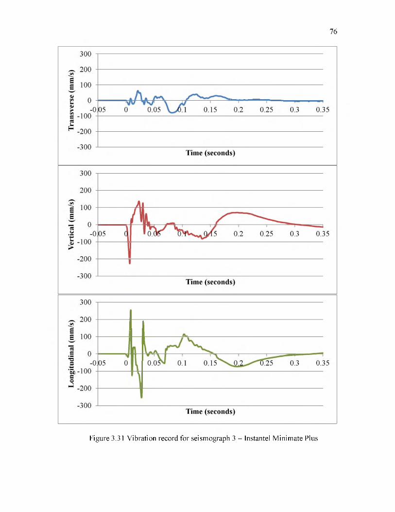
76

Figure 3.31 Vibration record for seismograph 3 - Instantel Minimate Plus

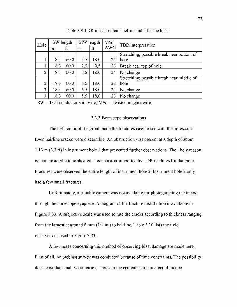
77

Table 3.9 TDR measurements before and after the blast

HoleSW length MW ength MW

AWGTDR interpretation

m ft m ft

1 18.3 60.0 5.5 18.0 24Stretching; possible break near bottom of hole

1 18.3 60.0 2.9 9.5 28 Break near top of hole2 18.3 60.0 5.5 18.0 24 No change

2 18.3 60.0 5.5 18.0 28Stretching; possible break near middle of hole

3 18.3 60.0 5.5 18.0 24 No change3 18.3 60.0 5.5 18.0 28 No change

SW - Two-conductor shot wire; MW - Twisted magnet wire

3.3.3 Borescope observations

The light color of the grout made the fractures easy to see with the borescope.

Even hairline cracks were discernible. An obstruction was present at a depth of about

1.13 m (3.7 ft) in instrument hole 1 that prevented further observations. The likely reason

is that the acrylic tube sheared, a conclusion supported by TDR readings for that hole.

Fractures were observed the entire length of instrument hole 2. Instrument hole 3 only

had a few small fractures.

Unfortunately, a suitable camera was not available for photographing the image

through the borescope eyepiece. A diagram of the fracture distribution is available in

Figure 3.33. A subjective scale was used to rate the cracks according to thickness ranging

from the largest at around 6 mm (1/4 in.) to hairline. Table 3.10 lists the field

observations used in Figure 3.33.

A few notes concerning this method of observing blast damage are made here.

First of all, no preblast survey was conducted because of time constraints. The possibility

does exist that small volumetric changes in the cement as it cured could induce

Inst

rum

ent

hole

3 In

stru

men

t ho

le 2

Inst

rum

ent

hole

1

78

MW - magnet wire SW - shot wire

Figure 3.32 Digitized TDR signatures

79

Figure 3.33 Fracture distribution observed with borescope

80

Table 3.10 Field notes of crack observations

HoleDepth below collar

NotesMeters Feet

1 0.85 2.20 Start of fracture zone1 0.98 2.80 End of fracture zone1 1.13 3.20 Shearing of tube2 0.61 3.70 Very large crack2 1.02 2.00 Large crack2 2.06 3.35 Small crack2 2.30 6.75 Small crack2 2.64 7.55 Small crack2 3.31 8.65 Two small cracks2 3.37 10.85 Start of fracture zone/large cracks2 3.43 11.05 End of fracture zone/large cracks2 3.76 11.25 Large crack2 4.07 12.35 Two small cracks2 4.13 13.35 Medium crack + small crack2 4.16 13.55 Small crack3 0.89 13.65 Medium crack3 1.07 2.91 Small crack3 2.53 3.51 Small crack3 2.75 8.31 Very small crack

cracking. However, Hydro-Stone™ has a maximum setting expansion of only 0.24%.

The pattern of fractures observed does not suggest any cracking in the grout from

volumetric changes. Thus the likelihood of cracking during the setting phase is unlikely.

It is possible that the stress wave may have induced fractures in the cement itself.

The HydroStoneTM datasheet did not list material properties other than compressive

strength. However, the HydroStone™ does not appear as brittle or stiff as the rhyolite and

as such would be less prone to tensile fracture. The movement of joint sets or preexisting

fractures at the test site could also cause cracking in the cement, possibly even at a

distance beyond the limit of tensile fracturing in the rhyolite. No data was available,

though, on joint set distribution, so this possibility could not be verified.

Yang et al. (1993) pointed out that observation holes in the near field filled with

grout could cause impedance mismatches for wave propagation if the rock and cement

possess different properties. This consideration was not made for the field experiment, so

its potential effect on the data collected are not known. An interesting exercise would be

to conduct a numerical simulation of this problem and analyze the results. That is beyond

the scope of this work, however.

3.3.4 Visual observations

Cracks appeared in the ground surface opposite the instrument holes. The ground

was sloped downwards on this particular side, possibly making it a more favorable

pathway for high-pressure gases to escape in addition to reflection of surface waves.

Figure 3.34 is a photo taken of the cracks.

3.3.5 Summary of results

The borescope provided the best means by which to determine damage in the rock

surrounding the explosive charge. Fracturing of the rock was observed up to 3.78 m (12.4

ft) from the blasthole. Significant fracturing was observed within 2.10 m (6.9 ft) of the

blasthole. The necessary setup to employ this method is relatively inexpensive and easy

to apply in the field. The only expensive component is the borescope itself, which must

be equipped with a built-in light source.

Measurements taken using time-domain reflectometry seem to corroborate

observations with the borescope. However, the TDR measurements in themselves lack

81

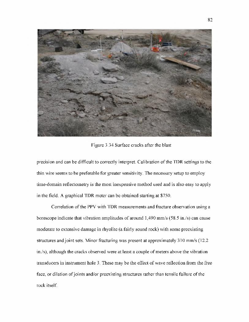
82

Figure 3.34 Surface cracks after the blast

precision and can be difficult to correctly interpret. Calibration of the TDR settings to the

thin wire seems to be preferable for greater sensitivity. The necessary setup to employ

time-domain reflectometry is the most inexpensive method used and is also easy to apply

in the field. A graphical TDR meter can be obtained starting at $750.

Correlation of the PPV with TDR measurements and fracture observation using a

borescope indicate that vibration amplitudes of around 1,490 mm/s (58.5 in./s) can cause

moderate to extensive damage in rhyolite (a fairly sound rock) with some preexisting

structures and joint sets. Minor fracturing was present at approximately 310 mm/s (12.2

in./s), although the cracks observed were at least a couple of meters above the vibration

transducers in instrument hole 3. These may be the effect of wave reflection from the free

face, or dilation of joints and/or preexisting structures rather than tensile failure of the

rock itself.

The extent of damage in the rock mass was between 2.10 m (6.9 ft) and 3.78 m

(12.4 ft), with PPV in the region attenuating from 1,490 mm/s (58.5 in./s) to 310 mm/s

(12.2 in./s) in-line with the elevation of the explosive column. The measured PPV is

based on dilatational wave motion. Measurement of shear wave motion would require

triaxial vibration transducers to record transverse and vertical movement in addition to

longitudinal.

83

4. DAMAGE PREDICTION

Three methods were chosen for predicting the extent of damage from the

blasthole in the previous section. The purpose was two-fold: (1) to compare the

prediction models against each other and (2) to evaluate how well each model compares

to the field data. The three approaches selected were

• A modified Holmberg-Persson approach developed by Smith (2003),

• The shock wave transfer (SWT) model developed by Sun (2013), and

• Numerical simulation using ANSYS Autodyn™

4.1 Rhyolite properties

In order to employ predictive models, mechanical properties of the rhyolite rock

were needed. A suite of rock mechanics tests were conducted on a sample of rhyolite

obtained from the test site. Table 4.1 lists the results of the testing program. Details of the

tests are provided in Appendix E.

4.2 Modified Holmberg-Persson approach

Smith (2003) took the least squares method (LSM) approach presented in Section

B.4.3 for the scaled distance method and adapted it for the Holmberg-Persson (HP)

model. The goal is to minimize the sum of the residuals squared SRS between measured

and predicted vibrations. Mathematically, this is expressed as

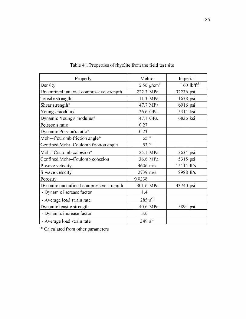
85

Table 4.1 Properties of rhyolite from the field test site

Property Metric ImperialDensity 2.56 g/cm3 160 lb/ft3Unconfined uniaxial compressive strength 222.3 MPa 32236 psiTensile strength 11.3 MPa 1638 psiShear strength* 47.7 MPa 6916 psiYoung's modulus 36.6 GPa 5311 ksiDynamic Young's modulus* 47.1 GPa 6836 ksiPoisson's ratio 0.27Dynamic Poisson's ratio* 0.23Moh—Coulomb friction angle* 65 °Confined Mohr-Coulomb friction angle 53 °

Mohr-Coulomb cohesion* 25.1 MPa 3634 psiConfined Mohr-Coulomb cohesion 36.6 MPa 5315 psiP-wave velocity 4606 m/s 15111 ft/sS-wave velocity 2739 m/s 8988 ft/sPorosity 0.0238Dynamic unconfined compressive strength 301.6 MPa 43740 psi- Dynamic increase factor 1.4

- Average load strain rate 285 s-1Dynamic tensile strength 40.6 MPa 5894 psi- Dynamic increase factor 3.6

- Average load strain rate 349 s-1

* Calculated from other parameters

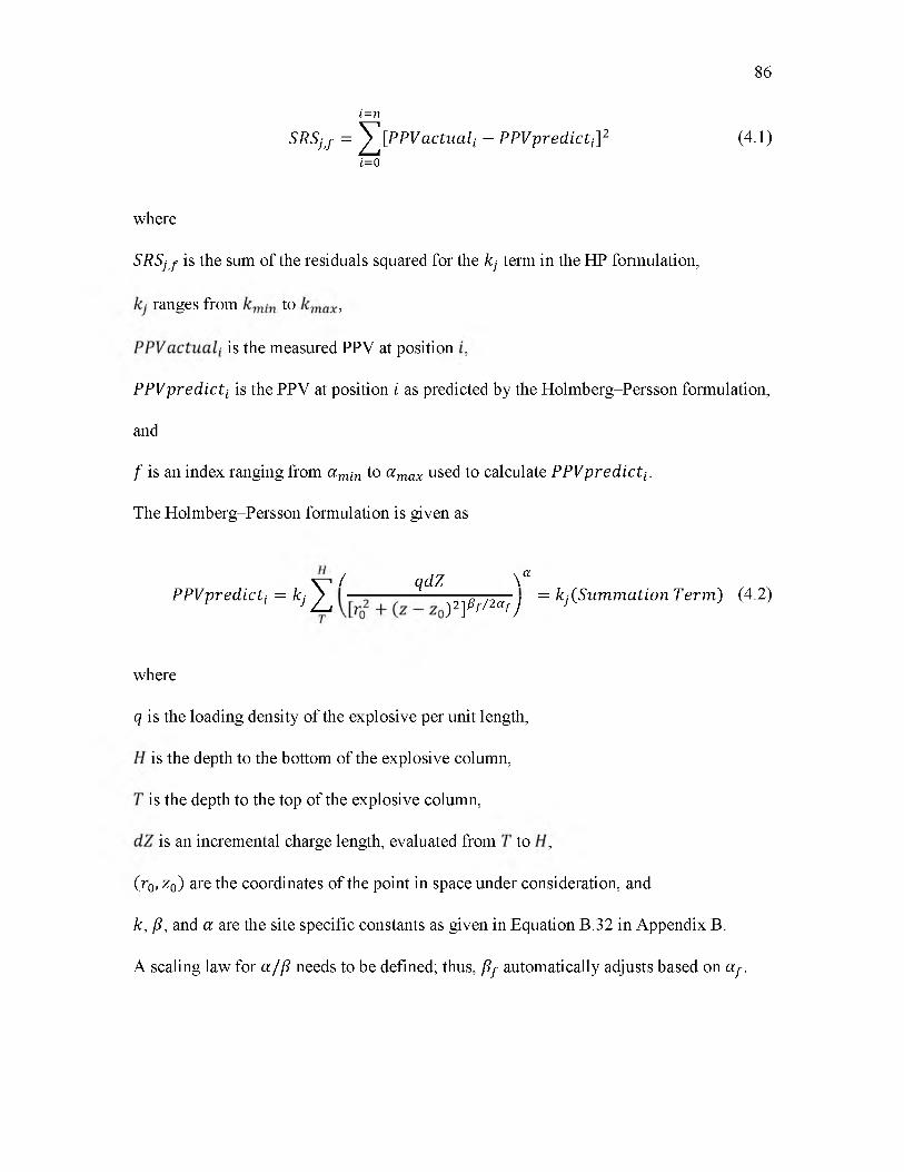
i=n

S R S j j = ^ [ P P V a c tu a I i — P P Vp r e d i c t J 2 (4.1)i=o

where

SR Syj- is the sum of the residuals squared for the kj term in the HP formulation,

ranges from to ,

is the measured PPV at position ,

P P Vpr e d i c t is the PPV at position i as predicted by the Holmberg-Persson formulation,

and

f is an index ranging from amin to amax used to calculate P P Vp r e d i c t j.

The Holmberg-Persson formulation is given as

v -1 / qdZ \ a PPVpredicti = kj ^ — --------- ^2^Pf/2af J = kj(.Summation Term) (4.2)

where

q is the loading density of the explosive per unit length,

is the depth to the bottom of the explosive column,

is the depth to the top of the explosive column,

is an incremental charge length, evaluated from to ,

(r0, z 0) are the coordinates of the point in space under consideration, and

k, /?, and a are the site specific constants as given in Equation B.32 in Appendix B.

A scaling law for a / / needs to be defined; thus, / f automatically adjusts based on af.

86

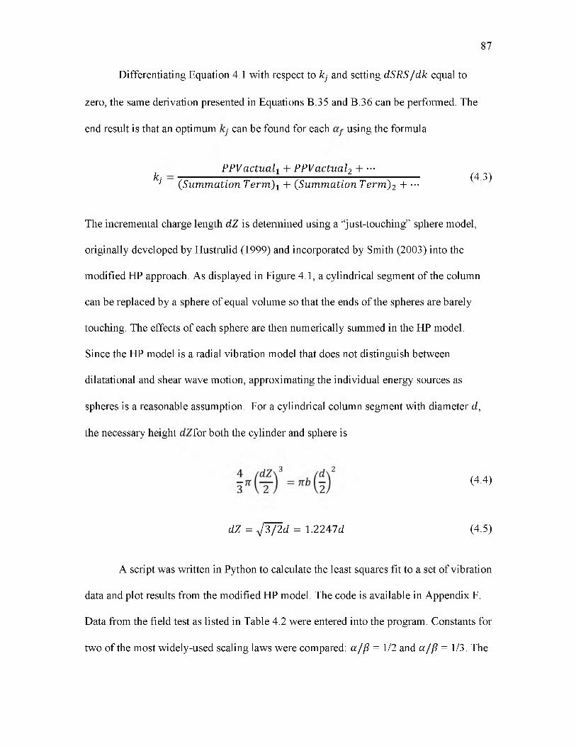
Differentiating Equation 4.1 with respect to kj and setting dSRS/ dk equal to

zero, the same derivation presented in Equations B.35 and B.36 can be performed. The

end result is that an optimum can be found for each using the formula

87

PPVactual-L + PPVactual2 + ••• kj (Summation Term)t + (Summation Term)2 + ■ ■ ■ (43)

The incremental charge length dZ is determined using a “just-touching” sphere model,

originally developed by Hustrulid (1999) and incorporated by Smith (2003) into the

modified HP approach. As displayed in Figure 4.1, a cylindrical segment of the column

can be replaced by a sphere of equal volume so that the ends of the spheres are barely

touching. The effects of each sphere are then numerically summed in the HP model.

Since the HP model is a radial vibration model that does not distinguish between

dilatational and shear wave motion, approximating the individual energy sources as

spheres is a reasonable assumption. For a cylindrical column segment with diameter d,

the necessary height for both the cylinder and sphere is

(44)

dZ = j r / i d = 1.2 247d (4.5)

A script was written in Python to calculate the least squares fit to a set of vibration

data and plot results from the modified HP model. The code is available in Appendix F.

Data from the field test as listed in Table 4.2 were entered into the program. Constants for

two of the most widely-used scaling laws were compared: a / (3 = 1/2 and a / fi = 1/3. The

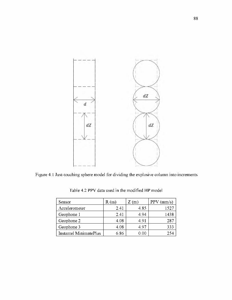
88

Figure 4.1 Just-touching sphere model for dividing the explosive column into increments

Table 4.2 PPV data used in the modified HP model

Sensor R (m) Z (m) PPV (mm/s)Accelerometer 2.41 4.85 1527Geophone 1 2.41 4.94 1438Geophone 2 4.08 4.91 287Geophone 3 4.08 4.97 333Instantel MinimatePlus 6.86 0.00 254

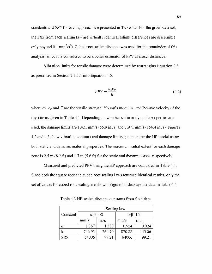
constants and SRS for each approach are presented in Table 4.3. For the given data set,

the from each scaling law are virtually identical (slight differences are discernible

2 2only beyond 0.1 mm /s ). Cubed root scaled distance was used for the remainder of this

analysis, since it is considered to be a better estimator of PPV at closer distances.

Vibration limits for tensile damage were determined by rearranging Equation 2.3

as presented in Section 2.1.1.1 into Equation 4.6:

Gt-CpP p V = (4.6)

E

where <rt , c P and E are the tensile strength, Young’s modulus, and P-wave velocity of the

rhyolite as given in Table 4.1. Depending on whether static or dynamic properties are

used, the damage limits are 1,421 mm/s (55.9 in./s) and 3,971 mm/s (156.4 in./s). Figures

4.2 and 4.3 show vibration contours and damage limits generated by the HP model using

both static and dynamic material properties. The maximum radial extent for each damage

zone is 2.5 m (8.2 ft) and 1.7 m (5.6 ft) for the static and dynamic cases, respectively.

Measured and predicted PPV using the HP approach are compared in Table 4.4.

Since both the square root and cubed root scaling laws returned identical results, only the

set of values for cubed root scaling are shown. Figure 4.4 displays the data in Table 4.4,

89

Table 4.3 HP scaled distance constants from field data

ConstantScaling law

o/p=1/2 o/p=1/3mm/s in./s mm/s in./s

a 1.387 1.387 0.924 0.924k 746.93 264.79 870.88 445.06SRS 64006 99.21 64006 99.21

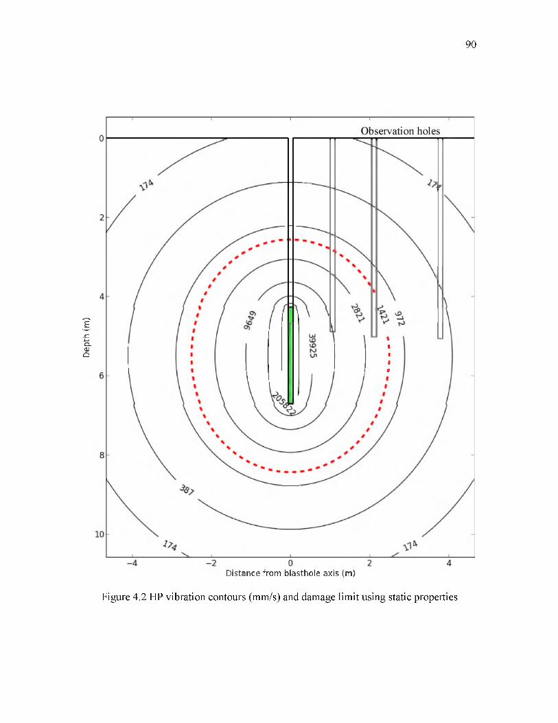
Dept

h (m

)

90

Distance from blasthole axis (m)

Figure 4.2 HP vibration contours (mm/s) and damage limit using static properties

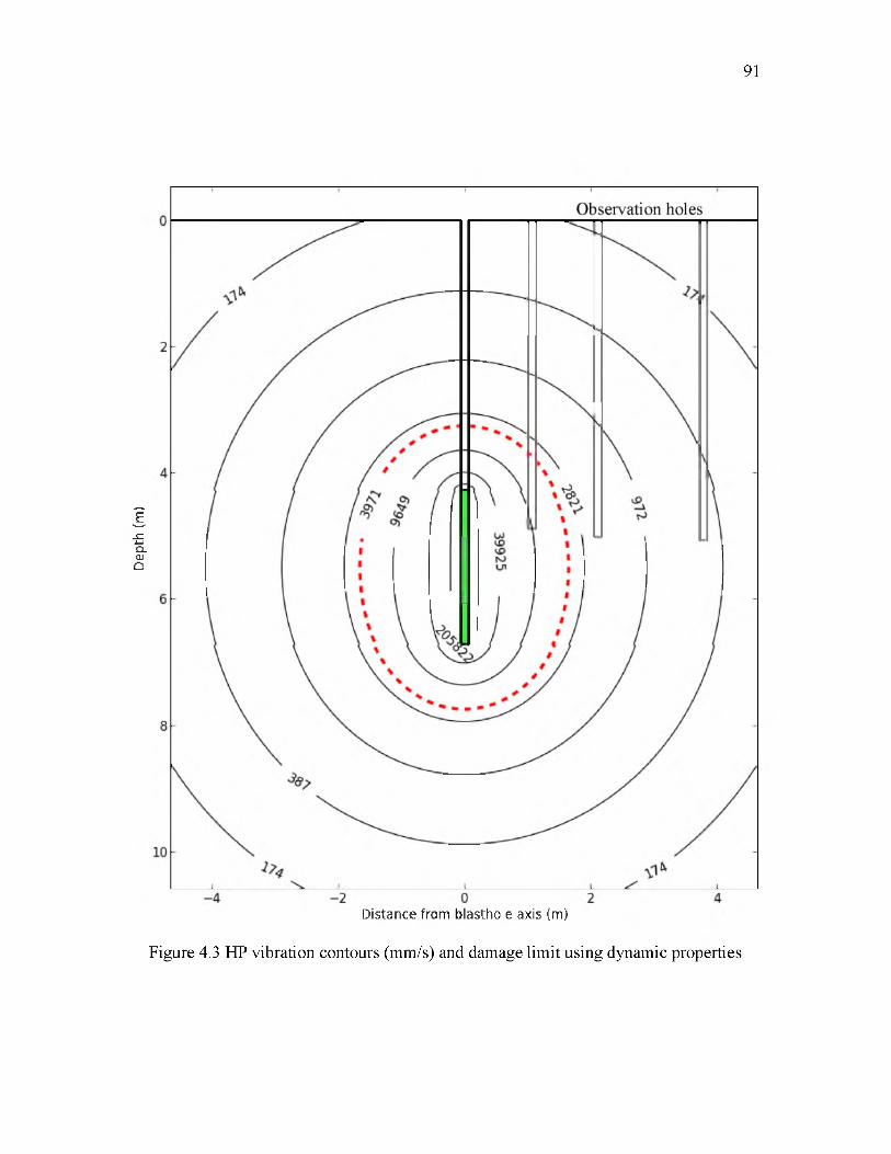
Dept

h (m

)

91

Distance from blasthole axis (m)

Figure 4.3 HP vibration contours (mm/s) and damage limit using dynamic properties

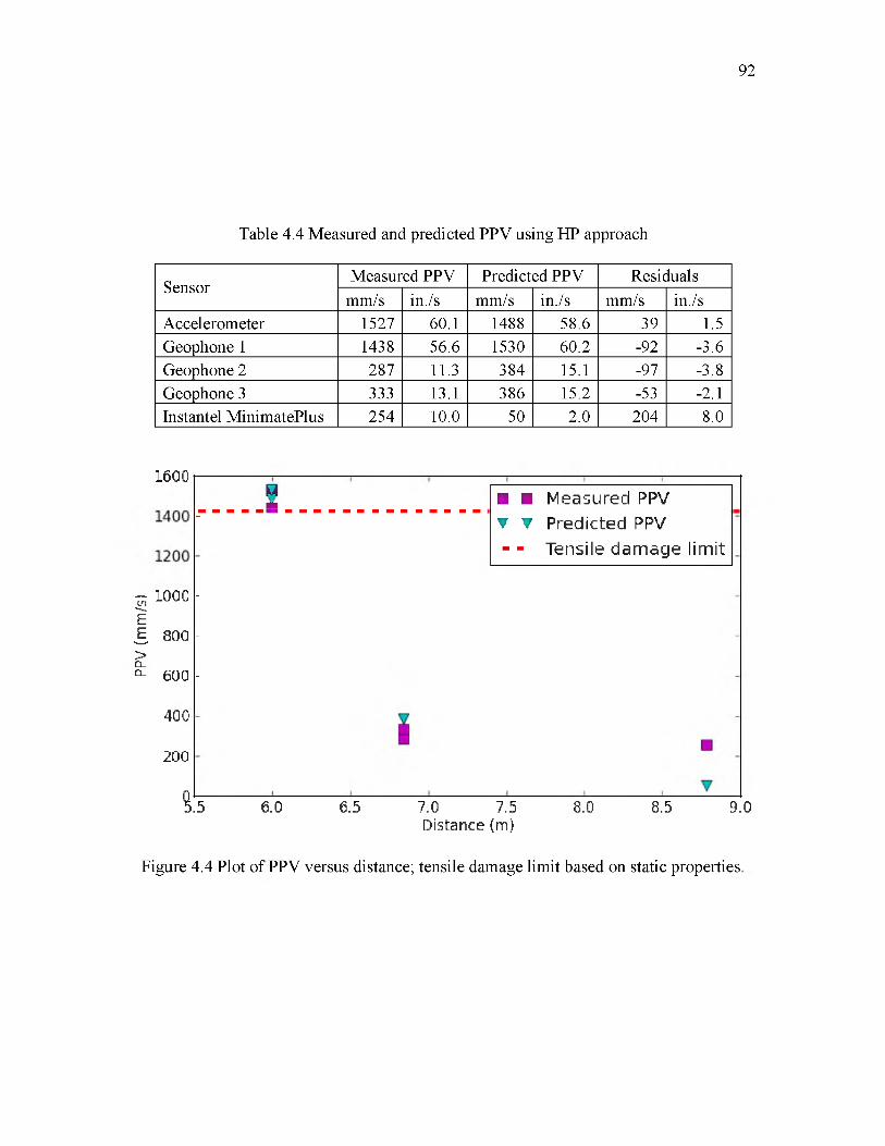
PPV

(mm

/s)

92

Table 4.4 Measured and predicted PPV using HP approach

SensorMeasured PPV Predicted PPV Residuals

mm/s in./s mm/s in./s mm/s in./sAccelerometer 1527 60.1 1488 58.6 39 1.5Geophone 1 1438 56.6 1530 60.2 -92 -3.6Geophone 2 287 11.3 384 15.1 -97 -3.8Geophone 3 333 13.1 386 15.2 -53 -2.1Instantel MinimatePlus 254 10.0 50 2.0 204 8.0

1600 [II ■ ■ Measured PPV" ▼ ▼ Predicted PPV

- - Tensile dam age lim it

1000 -

800 -

600 -

400

200

?.5 6.0 6.5 7.0 7.5 8.0 8.5 9.0Distance (m)

Figure 4.4 Plot of PPV versus distance; tensile damage limit based on static properties

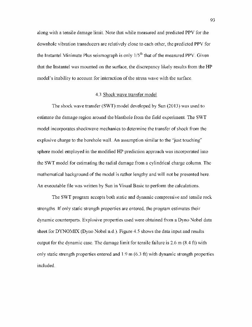
along with a tensile damage limit. Note that while measured and predicted PPV for the

downhole vibration transducers are relatively close to each other, the predicted PPV for

the Instantel Minimate Plus seismograph is only 1/5th that of the measured PPV. Given

that the Instantel was mounted on the surface, the discrepancy likely results from the HP

model’s inability to account for interaction of the stress wave with the surface.

4.3 Shock wave transfer model

The shock wave transfer (SWT) model developed by Sun (2013) was used to

estimate the damage region around the blasthole from the field experiment. The SWT

model incorporates shockwave mechanics to determine the transfer of shock from the

explosive charge to the borehole wall. An assumption similar to the “just touching”

sphere model employed in the modified HP prediction approach was incorporated into

the SWT model for estimating the radial damage from a cylindrical charge column. The

mathematical background of the model is rather lengthy and will not be presented here.

An executable file was written by Sun in Visual Basic to perform the calculations.

The SWT program accepts both static and dynamic compressive and tensile rock

strengths. If only static strength properties are entered, the program estimates their

dynamic counterparts. Explosive properties used were obtained from a Dyno Nobel data

sheet for DYNOMIX (Dyno Nobel n.d.). Figure 4.5 shows the data input and results

output for the dynamic case. The damage limit for tensile failure is 2.6 m (8.4 ft) with

only static strength properties entered and 1.9 m (6.3 ft) with dynamic strength properties

included.

93

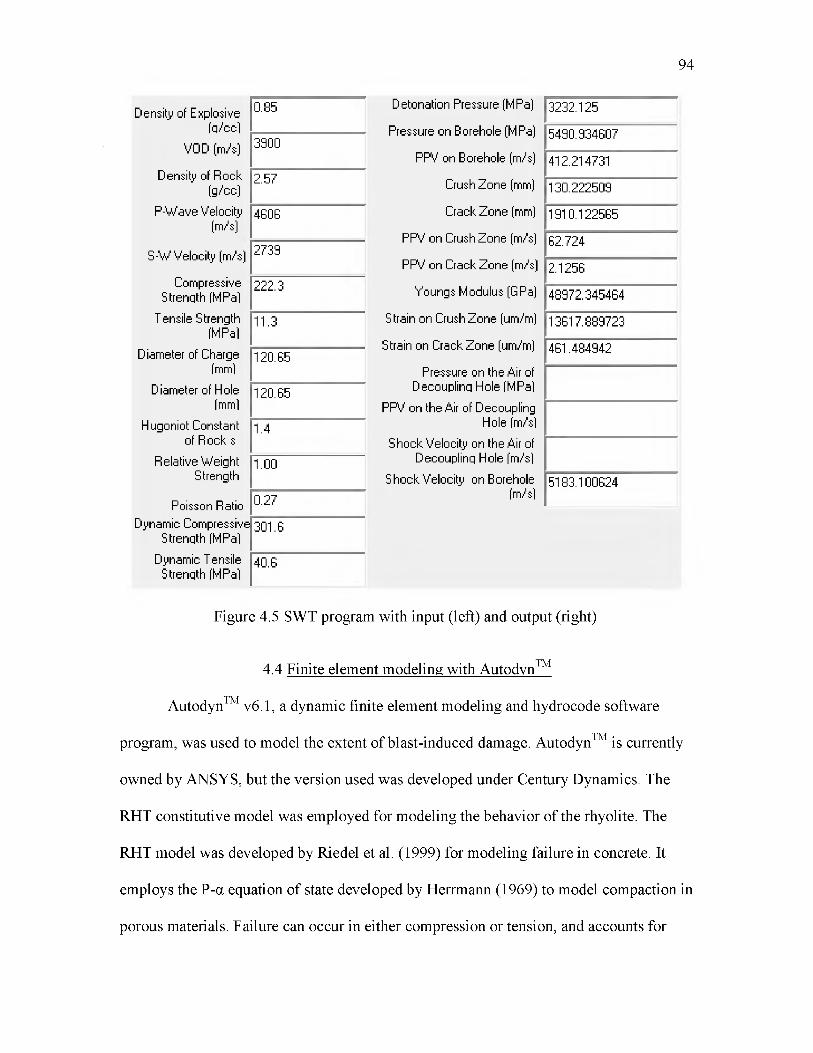
94

Density of Explosive (q /cc l

0.85

VOD (m/s) 3300

Density of Rock (g/cc)

2.57

P-Wave Velocity (m/s)

4606

S-W Velocity (m/s) 2739

Compressive Strength (MPa)

222.3

Tensile Strength (MPal

11.3

Diameter of Charge (mm)

120.65

Diameter of Hole fmml

120.65

Hugoniot Constant of Rock s

1.4

Relative W eight Strength

1.00

Poisson Ratio 0.27

Dynamic Compressive Strength (MPa)

301.6

Dynamic T ensile Strength (MPa)

40.6

Detonation Pressure (MPa)

Pressure on Borehole (MPa)

PPV on Borehole (m/s)

Crush Zone (mm)

Crack Zone (mm)

PPV on Crush Zone (m/s)

PPV on Crack Zone (m/s)

Youngs Modulus (GPa)

Strain on Crush Zone (urn/m)

Strain on Crack Zone (urn/m)

Pressure on the Air of Decouplinq Hole fMPal

PPV on the Air of Decoupling Hole fm/sl

Shock Velocity on the Air of Decouplinq Hole (m/sl

Shock Velocity on Borehole (m/sl

3232.125

5430.934607

412.214731

130.222503

1310.122565

62.724

2.1256

48972.345464

13617.SS9723

461.4S4S42

5133.100624

Figure 4.5 SWT program with input (left) and output (right)

TM4.4 Finite element modeling with Autodyn

Autodyn™ v6.1, a dynamic finite element modeling and hydrocode software

program, was used to model the extent of blast-induced damage. Autodyn™ is currently

owned by ANSYS, but the version used was developed under Century Dynamics. The

RHT constitutive model was employed for modeling the behavior of the rhyolite. The

RHT model was developed by Riedel et al. (1999) for modeling failure in concrete. It

employs the P-a equation of state developed by Herrmann (1969) to model compaction in

porous materials. Failure can occur in either compression or tension, and accounts for

phenomenon such as strain hardening, damage accumulation, strain softening from

damage, and porous collapse. Several published numerical investigations on rock blasting

have employed the RHT model in Autodyn™ such as Katsabanis (2005), Park and Jeon

(2010), Preece and Chung (2003), and Preece and Lownds (2008).

A two-dimensional axisymmetric model was created in Autodyn™ to simulate the

blasthole employed in the field test, shown in Figure 4.6. The axis of symmetry runs

through the center of blasthole. Two meshes with uniform element sizes were used: a

Lagrangian mesh for the rhyolite and an Eulerian mesh for the ANFO, air, and stemming.

The Lagrangian mesh was set at 12.80 m (42.0 ft) with 1,008 elements in the x-direction

and 6.03 m (19.8 ft) with 500 elements in the y-direction. The Eulerian mesh was set at

14.33 m (47.0 ft) with 1,128 elements in the x-direction and 6.03 m (19.8 ft) with 500

elements in the y-direction. The additional 1.52 m (5.0 ft) above the surface was added to

allow the gases and stemming to vent out of the blasthole. A total of 504,000 elements

were contained in the Lagrangian mesh and 564,000 cells in the Eulerian mesh. The

95

Figure 4.6 Autodyn model with gauge points displayed

individual element dimensions were 1.27 cm in the x-direction and 1.2065 cm in the y-

direction. The dimension in the x-direction was selected to be a whole multiple of a foot

and to avoid poor element shape factors in the conjunction with the y-dimension. The

dimension in the y-direction was selected so that five elements would span the radius of

the blasthole, a recommendation made by D.S. Preece (personal communication). The

default units were set at cm, ms, and g.

For stemming, sand was selected to simulate drill cuttings. Void space was

defined in the region outside the blasthole and beneath the surface. Interaction between

the Lagrangian and Eulerian meshes was enabled. A transmitting boundary was defined

at the sides and base of both meshes, and at the top of the Eulerian mesh. The point of

detonation was specified at the midpoint of the ANFO column. Gauge points 1 and 2

were placed at the two locations where the downhole vibration transducers were secured

in the field test. Gauge points 3 and 4 were placed at the edges of the model to check for

any reflections from the transmitting boundaries.

4.4.1 Material properties

Autodyn™ possesses a library with properties, equations of state, constitutive

models, and failure criteria for a wide variety of materials. For rhyolite, a concrete

material labeled CONC140MPA was selected. Certain material parameters were

modified to reflect the rhyolite properties measured during the rock mechanics testing

program, as listed in Table 4.5. Shear modulus G was calculated from Young’s modulus

E and Poisson’s ratio v using the formula

96

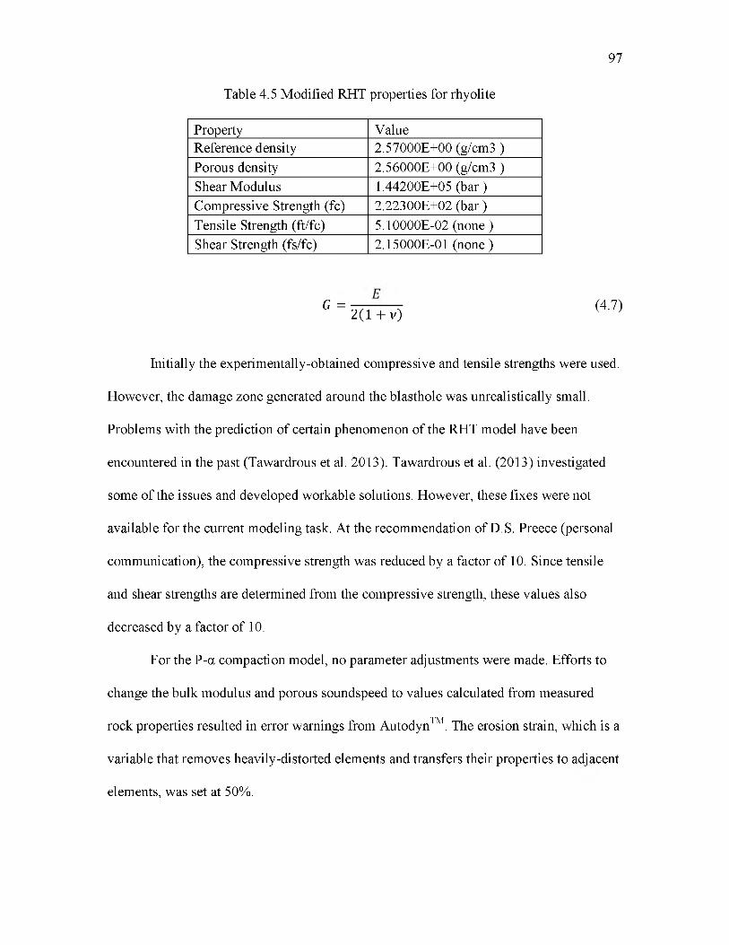
97

Table 4.5 Modified RHT properties for rhyolite

Property ValueReference density 2.57000E+00 (g/cm3 )Porous density 2.56000E+00 (g/cm3 )Shear Modulus 1.44200E+05 (bar )Compressive Strength (fc) 2.22300E+02 (bar )Tensile Strength (ft/fc) 5.10000E-02 (none )Shear Strength (fs/fc) 2.15000E-01 (none )

G =2 ( 1 + v )

(4.7)

Initially the experimentally-obtained compressive and tensile strengths were used.

However, the damage zone generated around the blasthole was unrealistically small.

Problems with the prediction of certain phenomenon of the RHT model have been

encountered in the past (Tawardrous et al. 2013). Tawardrous et al. (2013) investigated

some of the issues and developed workable solutions. However, these fixes were not

available for the current modeling task. At the recommendation of D.S. Preece (personal

communication), the compressive strength was reduced by a factor of 10. Since tensile

and shear strengths are determined from the compressive strength, these values also

decreased by a factor of 10.

For the P-a compaction model, no parameter adjustments were made. Efforts to

change the bulk modulus and porous soundspeed to values calculated from measured

rock properties resulted in error warnings from AutodynTM. The erosion strain, which is a

variable that removes heavily-distorted elements and transfers their properties to adjacent

elements, was set at 50%.

ANFO was selected from the Autodyn™ material library. The JWL equation of

state, developed by Lee et al. (1968), was employed. The density was changed to 0.85

g/cm , and the density cut-off was set to a value of 1E-4 to avoid small timesteps as the

gaseous products vented from the blasthole.

Sand was selected from the Autodyn™ material library. A porous compaction

model was employed, in which the properties of sand are specified for a set of pressures.

The erosion strain was set to 100%.

Air was modeled as an ideal gas using the AutodynTM material library reference.

When filling a region of the model with air, Autodyn requires that the internal energy be

specified. The specific internal energy of air uair was determined to be 2.163E+03 erg/g

using the thermodynamic relationship uair = cvT, where cv = 0.721 kJ/kg is the constant

volume specific heat capacity of air, and the temperature T was chosen as 300 K (27° F).

For all of the materials, the maximum soundspeed cutoff was lowered to avoid

small timesteps. The internal energy transport option was selected for Euler grid

calculations to avoid Euler cell errors that occurred using total energy transport. Detailed

material properties can be found in Appendix G.

4.4.2 Simulation results

The model took about six days for a 3.0 GHz 32-bit desktop to calculate the first

20 ms of simulation time. Since an older version of Autodyn™ was used, parallel

processing capability was not supported. The progression of damage around the blasthole

is shown in Figure 4.7. The RHT model employs a cumulative damage scale that ranges

between 0.0 for intact rock and 1.0 for rock that has undergone total failure. Small

regions of mild damage were observed at the boundaries below and to the sides of the

98

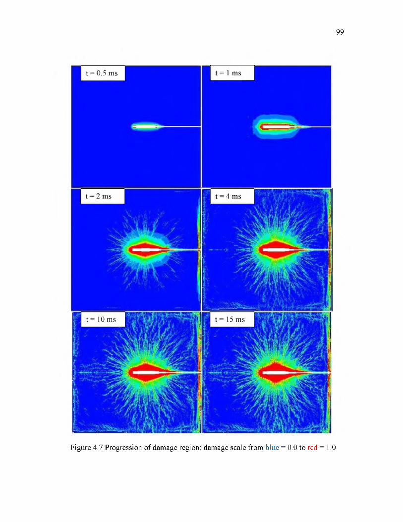
99

Figure 4.7 Progression of damage region; damage scale from blue = 0.0 to red = 1.0

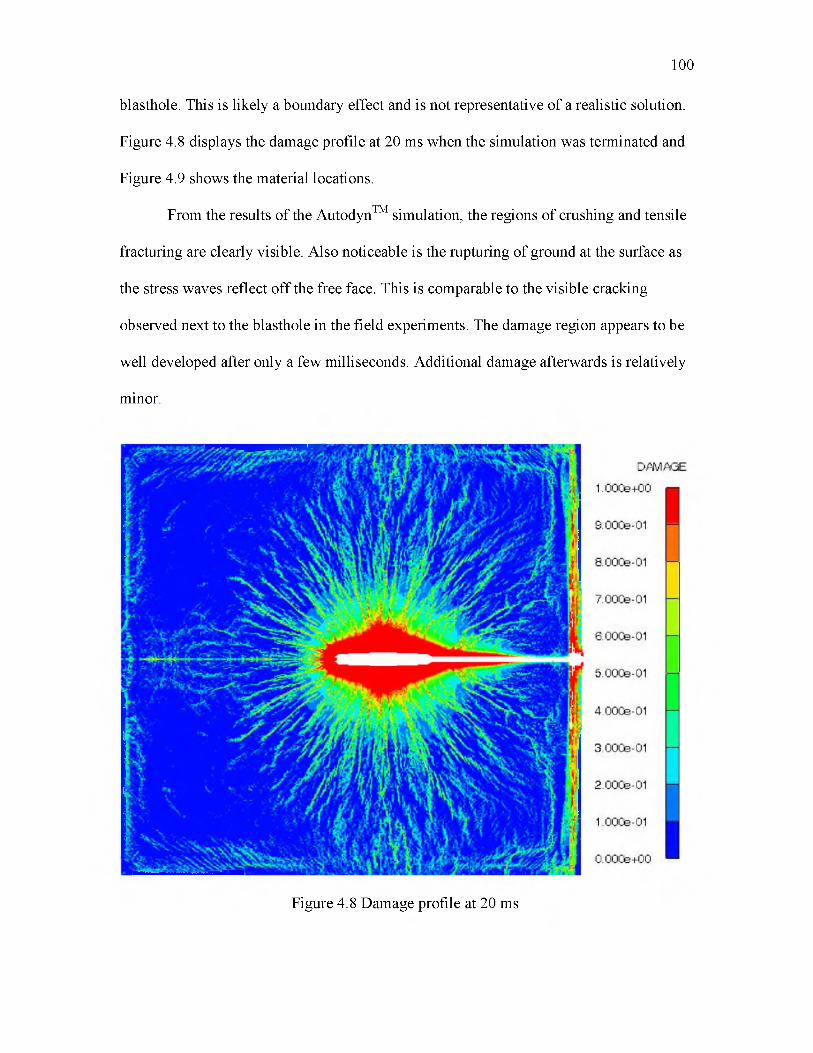
blasthole. This is likely a boundary effect and is not representative of a realistic solution.

Figure 4.8 displays the damage profile at 20 ms when the simulation was terminated and

Figure 4.9 shows the material locations.

From the results of the Autodyn™ simulation, the regions of crushing and tensile

fracturing are clearly visible. Also noticeable is the rupturing of ground at the surface as

the stress waves reflect off the free face. This is comparable to the visible cracking

observed next to the blasthole in the field experiments. The damage region appears to be

well developed after only a few milliseconds. Additional damage afterwards is relatively

minor.

100

Figure 4.8 Damage profile at 20 ms

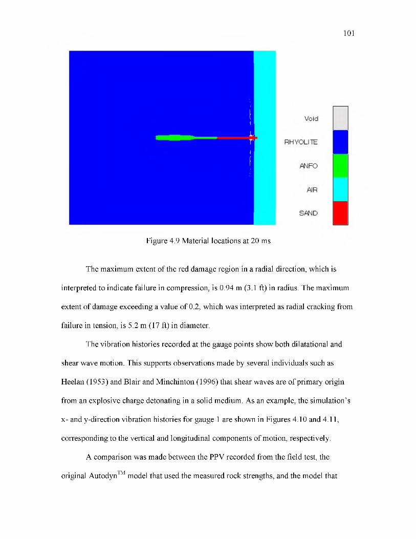
Figure 4.9 Material locations at 20 ms

The maximum extent of the red damage region in a radial direction, which is

interpreted to indicate failure in compression, is 0.94 m (3.1 ft) in radius. The maximum

extent of damage exceeding a value of 0.2, which was interpreted as radial cracking from

failure in tension, is 5.2 m (17 ft) in diameter.

The vibration histories recorded at the gauge points show both dilatational and

shear wave motion. This supports observations made by several individuals such as

Heelan (1953) and Blair and Minchinton (1996) that shear waves are of primary origin

from an explosive charge detonating in a solid medium. As an example, the simulation’s

x- and y-direction vibration histories for gauge 1 are shown in Figures 4.10 and 4.11,

corresponding to the vertical and longitudinal components of motion, respectively.

A comparison was made between the PPV recorded from the field test, the

original AutodynTM model that used the measured rock strengths, and the model that

101

102

Figure 4.10 Vertical vibration history at gauge 1

Figure 4.11 Longitudinal vibration history at gauge 1

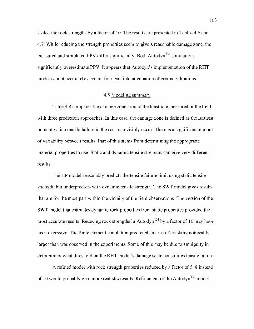
scaled the rock strengths by a factor of 10. The results are presented in Tables 4.6 and

4.7. While reducing the strength properties seem to give a reasonable damage zone, the

measured and simulated PPV differ significantly. Both AutodynTM simulations

significantly overestimate PPV. It appears that Autodyn’s implementation of the RHT

model cannot accurately account for near-field attenuation of ground vibrations.

4.5 Modeling summary

Table 4.8 compares the damage zone around the blasthole measured in the field

with three prediction approaches. In this case, the damage zone is defined as the furthest

point at which tensile failure in the rock can visibly occur. There is a significant amount

of variability between results. Part of this stems from determining the appropriate

material properties to use. Static and dynamic tensile strengths can give very different

results.

The HP model reasonably predicts the tensile failure limit using static tensile

strength, but underpredicts with dynamic tensile strength. The SWT model gives results

that are for the most part within the vicinity of the field observations. The version of the

SWT model that estimates dynamic rock properties from static properties provided the

most accurate results. Reducing rock strengths in Autodyn™ by a factor of 10 may have

been excessive. The finite element simulation predicted an area of cracking noticeably

larger than was observed in the experiments. Some of this may be due to ambiguity in

determining what threshold on the RHT model’s damage scale constitutes tensile failure.

A refined model with rock strength properties reduced by a factor of 5-8 instead

of 10 would probably give more realistic results. Refinement of the Autodyn™ model

103

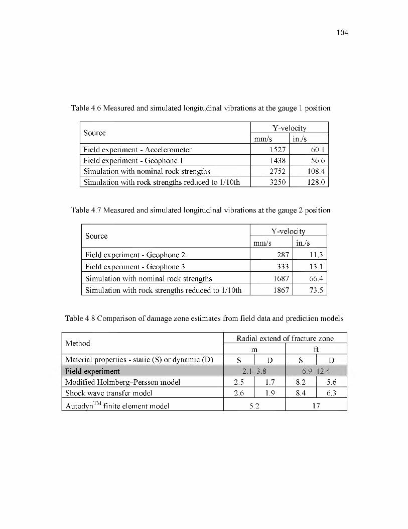
104

Table 4.6 Measured and simulated longitudinal vibrations at the gauge 1 position

SourceY-ve ocity

mm/s in./sField experiment - Accelerometer 1527 60.1Field experiment - Geophone 1 1438 56.6Simulation with nominal rock strengths 2752 108.4Simulation with rock strengths reduced to 1/10th 3250 128.0

Table 4.7 Measured and simulated longitudinal vibrations at the gauge 2 position

Source Y-velocitymm/s in./s

Field experiment - Geophone 2 287 11.3Field experiment - Geophone 3 333 13.1Simulation with nominal rock strengths 1687 66.4Simulation with rock strengths reduced to 1/10th 1867 73.5

Table 4.8 Comparison of damage zone estimates from field data and prediction models

Method Radial extend of fracture zonem ft

Material properties - static (S) or dynamic (D) S D S DField experiment 2.1-3.8 6.9-12.4Modified Holmberg-Persson model 2.5 1.7 8.2 5.6Shock wave transfer model 2.6 1.9 8.4 6.3

Autodyn™ finite element model 5.2 17

beyond the results shown here was considered outside the scope of this thesis and was

therefore not undertaken.

105

5. CONCLUSIONS AND RECOMMENDATIONS

5.1 Conclusions

A field experiment was performed to determine the extent of damage surrounding

a blasthole. A confined, cylindrical explosive charge was detonated in a body of

competent rhyolite rock. Measurements were conducted using three types of

instrumentation secured in nearby monitoring holes with grout. Near-field vibrations

were measured with unidirectional vibration transducers. Fractures were observed with a

borescope, lowered downhole through clear acrylic tubes that had previously been

grouted in place. Thin, two-conductor, twisted wires were grouted downhole to detect

shearing in the rock, and their continuity was measured with a time domain reflectometer

(TDR).

Three methods were used to predict the extent of the damage zone around the

blasthole: a modified Holmberg-Persson (HP) method developed by Smith (2003), a

shock wave transfer (SWT) model developed by Sun (2013), and a dynamic finite

element simulation using the commercial software program ANSYS Autodyn™. A

comparison was made between each approach and the field data, with damage defined as

the limit of tensile failure in the rock.

The following results and conclusions were found:

• Fracturing was observed downhole at radial distances up to 3.78 m (12.4

ft) from the blasthole. Moderate fracturing was observed 2.10 m (6.9 ft)

from the blasthole. Cracks were also visible on the ground surface

adjacent to the blasthole.

• Vibration measurements show significant fracturing occurring in the rock

mass at peak particle velocities (PPV) of 1,490 mm/s (58.5 in./s), but no

cracks at PPV of 310 mm/s (12.2 in./s). The limit of radial cracking for the

rhyolite lies between these two values. A tensile failure limit was

estimated to be 1,421 mm/s (55.9 in./s) from the relationship P P V =

at cP/E, where at is the tensile strength (in this case the static tensile

strength), cP is the P-wave velocity, and E is Young’s modulus of the

rhyolite. This vibration level possibly occurred only a short distance

beyond the monitoring hole 2.10 m (6.9 ft) from the blasthole.

• Cracks present in the grout surrounding the clear acrylic tubing were

easily observed with the borescope. Even hairline cracks were

distinguishable. A light-colored grout aided visibility.

• Rock displacement and shearing was detectable using a TDR and thin,

two-conductor, twisted wires. Of the two wire gauges used (24- and 28-

AWG), the 28-AWG wire was more sensitive to changes in the status of

the grout and thus more useful as a damage indicator. Impedance profiles

for each length of wire were difficult to interpret, however. Corroboration

with fracture observations was needed to better interpret results. Limits in

the resolution of the TDR instrument reduced the precision with which

events could be located. The TDR appears capable of detecting moderate

to significant damage, but not mild damage such as small fractures.

107

• The extent of the tensile failure damage limits estimated by each

prediction method employed were within the general vicinity of the field

observations, but varied widely. The modified HP model reasonably

predicted the damage limit using static material properties, but

underpredicted with dynamic material properties. The SWT method

predicted a reasonable damage limit using dynamic strength properties

estimated by the program from static strength properties. Entering

dynamic strength properties of the rock directly into the SWT program

slightly underpredicted the damage zone. The AutodynTM finite element

model overestimated the extent of the radial fracturing region. Strength

properties in the model were reduced by a factor of 10, however, to obtain

reasonable results with the RHT constitutive failure model. Calibration of

the model would likely result in a better estimate of the damage limit.

• Of all the methods that have been developed for predicting backbreak, it is

the author’s opinion that numerical methods hold the greatest potential.

Numerical models attempt to simulate the physics of the real world and

thus can account for factors that most others cannot, such as as free faces,

confinenment, and crack growth. Of the three damage prediction

approaches included in this thesis, only the AutodynTM simulation could

simulate interaction between the stress wave and the ground surface. The

HP and SWT models could not. The disadvantages in using numerical

methods is that they are complex and require a software package to

108

implement. Good modeling practice and model calibration is necessary to

obtain reasonable results.

5.2 Recommendations for further sturdy

Numerous field investigations have been conducted to determine the extent of

blast-induced damage, including single-hole blasts (for instance, see Smith [2003] and

Yang et al. [1993]). The field work conducted in this thesis provides a unique study of

damage around a blasthole using three forms of measurements: near-field vibrations, a

borehole fracture survey, and continuity testing with a TDR. To the author’s knowledge,

all three have never been used in conjunction with each other in the same experiment. In

addition, a new method to visually observe blast-induced fractures was developed. The

method can be easily implemented in the field at a low cost, although a borescope itself is

an expensive instrument. Several methods for estimating the size of the damage zone

around a blasthole were also applied and evaluated against the field measurements.

The research presented in this thesis brings to light several areas for additional

study and investigation. The following list presents a set of recommendations for future

research.

• To fully measure the motion of a rock body subject to blast loading,

triaxial vibration transducers should be employed. Knowing all three

components of vibrations can provide a better understanding of the modes

of vibration and the relative energies of each wave type. Uniaxial vibration

sensors were utilized in this study due to budgetary limitations. An

interesting study would be to compare vibration-based damage prediction

methods using a peak vector sum (PVS) of the three components of

109

motion. The author did not come across any near-field vibrations studies

that explicitly used a PVS; peak particle velocity tends to be the common

metric. A study using the PVS would require triaxial recording capability.

• Fracture surveying by grouting clear acrylic tubing down a monitoring

hole and observing cracking in the grout with a borescope proved to be

very successful. Ease of installation, relatively low cost, and clarity with

which fractures can be distinguished makes this survey method an

attractive and effective means to directly observe blast-induced damage.

Future studies of backbreak, both research and operations-oriented, could

employ this technique with a likely degree of success.

• The presence of a grout-filled hole adjacent to a blasthole could

potentially cause coupling problems or an impedance mismatch between

the grout and the surrounding rock. If so, the accuracy of measurements

taken by instruments secured in the grout might suffer. Cracking could

also occur in the grout itself but not in the adjacent rock. An area of

investigation would be to study the effects of the high-frequency

shockwave on a grout-filled hole in the vicinity of the explosive charge.

Numerical simulations and laboratory tests would be ideal, since the

testing conditions can be more easily controlled.

• No preblast fracture, fault, and joint-set mapping was performed for the

the experiment in this thesis. While not deemed critical due to the

competency of the rock outcrop at the test site, the possibility does exist

that some cracks observed in the grout may have been caused by shifting

110

along discontinuities in the rock rather than tensile failure. Mapping such

structures to correlate with postblast fracturing would require either a

preblast fracture survey with a downhole-camera or drilling and retrieving

core samples adjacent to the monitoring holes. Even then, attempts to find

a plausible correlation between blast-induced fracturing in the grouted

monitoring hole and shifting of the rock mass along preexisting structures

may not yield much useful information. Nonetheless, an in-depth study to

determine this particular aspect of the rock mass behavior on the grout

may be worthwhile. A field experiment similar to the one performed in

this thesis, instead conducted at a highly-fractured test site, may produce

observable cracking well beyond the limit of tensile failure in the rock.

• Time domain reflectometry using thin, two-conductor wires as employed

in this thesis may not be very informative nor useful for scientific

research, but its ease of installation and low cost make it a candidate for

incorporating into wall control studies at an active mining operation.

Moderate to significant damage can be detected behind a blast pattern.

Measurements with a TDR require little to no postprocessing, making it

useable by the average mine worker.

• Most publications on methods for predicting the extent of blast damage

include validation against field data. However, very little literature

reviewed by the author presents direct comparisons of mulitiple prediction

approaches against each other and field tests. This thesis used three

different prediction methods to estimate the zone of radial fracturing and

111

evaluated them against results from the experiment. A more extensive

study comparing, say, five to ten different prediction methods against field

results would provide a better understanding of the accuracy of each

method. Even a comparative analysis of several damage prediction models

against each other, without evaluation against a field test, might yield

valuable insight.

• The field experiment was conducted using a blasthole with much more

confinenment than is normally employed in practice. The goal of this

experiment was to obtain a worst-case scenario of backbreak. The

geometry of the test was expected to increase radial fracturing in

comparison with a normal blasthole. Future studies could focus on the

damage region from a typical production hole, which uses some

stemming, or a trim hole, which uses no stemming. The presence of a free

face on one side of the blasthole would be preferable. This would simulate

conditions from a normal shot where prior rows have already been fired,

leaving a free face adjacent to the last row.

112

APPENDIX A

THEORY OF ROCK BREAKAGE BY

EXPLOSIVES

An important requirement in studying any kind of physical process lies in

understanding the underlying theory. Blasting entails the interaction of complex physical

processes—processes, however, that are governed by fundamental principles. While

much research continues to be directed towards a more precise knowledge of these

processes, the general behavior of explosive-rock interaction during blasting is well

known.

The mechanisms by which explosives induce rock breakage are many and include

(Atlas Powder Company 1987) the following:

• Compressional and tensile shock wave and strain wave energy,

• Wave reflections at free faces and boundaries within the rock mass,

• High pressure gases acting on the surrounding rock mass,

• Flexural rupture,

• Shear waves,

• Release-of-load,

• Nucleation of cracks at preexisting flaws and discontinuities, and

• In-flight collisions.

There are four different stages in the blasting process (Atlas Powder Company

1987; Floyd 2008):

• Detonation of the explosive column,

• Shock and stress wave propagation,

• High pressure gas expansion, and

• Displacement of fragmented rock.

114

While each stage is distinct from the others, they are not necessarily sequential in

order of occurrence. They overlap and interact with each other to produce the final

product: fragmented and displaced rock.

A.1 Detonation of the explosive column

The first stage in the fragmentation process is the detonation of the explosive

charge to release its chemical energy. Detonation refers to a specific type of chemical

reaction; namely, one that propagates via a highly-energetic shock wave (Meyer et al.

2002). This is distinct from a similar process called deflagration in which the reaction

front propagates through thermal contact and radiation, such as occurs with burning

gasoline or propellants. Very large temperature and pressure gradients are formed, which

contribute to a very rapid rate of reaction. One-dimensional detonation theory dictates a

stable detonation front called the Chapman-Jouguet (CJ) plane. Immediately behind

exists the reaction zone, where the detonation pressure is generated. Figure A. 1 shows an

illustration of the CJ plane, reaction zones, and outgoing shockwave during the explosive

detonation process.

Detonation velocities range on the order of 1,500-9,100 m/s (5,000-30,000 ft/s).

At these velocities, a typical explosive column in a blasthole is consumed within several

milliseconds. In addition to explosive properties, the velocity of detonation (VOD) is also

dependent on degree of confinement and the diameter of the explosive charge (Atlas

Powder Company 1987). Higher explosive VODs release gaseous products more quickly,

resulting in higher pressures and are thus more suited for fragmenting hard rock. Lower

explosive VODs release gaseous products over a longer duration and thus perform better

in soft rock and applications that require greater heave of the blasted material.

115

116

For a well-confined explosive, the detonation pressure is given by

PD = Kpexp(VOD ) 2 (A.1)

where PD is the detonation pressure in kbar, K is a constant specific to the explosive, pexp

is the explosive density in g/cm3, and is in ft/s (Atlas Powder Company 1987). For

ANFO, K = 2.375E-7. Detonation pressures range on the order of 9,000-27,500 MPa (9­

275 kbar), with temperatures from 1,900-4,150 K (3,000-7,000 °F).

In transitioning to the next stage of rock breakage, the expansion of gaseous

products from the reaction zone apply a pressure along the walls of the borehole. Absent

117

an equation of state, the borehole pressure PB for a fully-coupled explosive is estimated

to be equal to one-half of the detonation pressure (Persson et al. 1994; McKenzie 1999).

Sun (2013) cautioned against using this simple approach, however, citing an analysis of

the shock wave transfer from the explosive to the borehole walls.

For a decoupled explosive, the borehole pressure is significantly less. If the

constant volume explosion pressures is known, the borehole pressure can be estimated

provided that the ratio y of the specific heat values cp and cv is known (y = cp/ cv)

(Persson et al. 1994). A typical value for y is on the order of 1.5.

where v is the specific volume of the explosive at the indicated state. For a unit length of

the blasthole, the specific volume only depends on the diameters of the borehole and

charges and , respectively.

McKenzie (1999) gave a relationship similar to Equation A.1 for computing the

Pb = Pd /2 (A.2)

(A.3)

(A.4)

borehole pressure but included a coupling factor fc, which is the ratio of the volume of

the explosive to the volume of the blasthole (minus the stemming column):

PB = 0 . 1 2fcnPexp(VOD ) 2 (A.5)

Here, is in Pa, is in kg/m3, is in m/sec, and is a coupling factor, usually

taken to be 1.2 to 1.3 for dry holes and 0.9 for saturated rock.

A.2 Shock and stress wave propagation

The second stage in fragmentation is the creation of a shock wave that propagates

outward from the borehole wall into the surrounding rock mass. The rapid decomposition

of the explosive into gaseous products generates extremely high pressures that are

transmitted to the borehole wall (Atlas Powder Company 1987; Floyd 2008). Within two

to three diameters of the blasthole, extensive crushing and/or plastic deformation of the

rock occurs as the dynamic compressive strength of the rock is exceeded. After the

pressure pulse applied by the explosive column peaks, it decays exponentially as the

borehole cavity expands and the gases cool. Figure A.2 shows the radial and tangential

stress decay at two different distances from the borehole. Field experiments by

Brinkmann (1990) produced borehole expansions ranging from 36% to 67%, depending

on the type of explosive used.

Beyond the pulverized zone of rock, the shock wave energy has diminished

enough such that the rock material no longer fails in compression, but can still fail in

shear and tension. The stress pulse traveling outwards compresses the rock and

simultaneously induces a tangential or “hoop” stress. The tangential stress component

induces tensile failure in the rock, which manifests itself in the form of cracks that extend

radially outwards. Studies indicate that the creation of these radially-formed cracks

occurs at a distance of about one blasthole diameter from the borehole wall (Persson et al.

1994). Initially, the density of radial fractures is high. Further out, the number of cracks

rapidly decreases as stress relaxation from fracturing favors the continuing extension of

118

119

Figure A.2 Generalized stress histories for two different distances R from blasthole (Source: Dowding and Aimone 1992. Reprinted with the permission of the Society for

Mining, Metallurgy, and Exploration; www.smenet.org).

only a few long cracks. Crack growth occurs until about 20-30 blasthole diameters from

the borehole wall (Floyd 2008). According to Oriard (1982), the extent of radial cracking

is controlled by

• Explosive energy,

• Rate of energy transmission to the adjacent rock, and

• Strength properties of the rock.

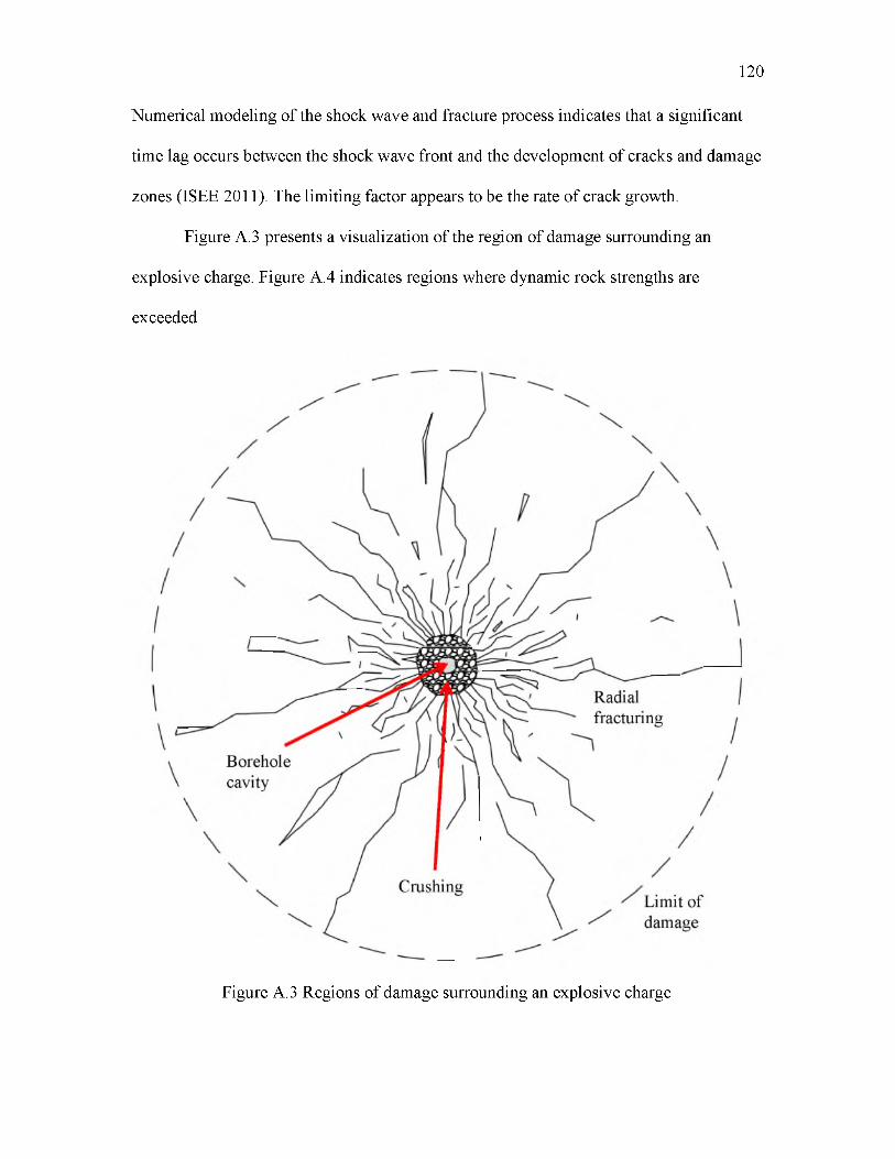
Numerical modeling of the shock wave and fracture process indicates that a significant

time lag occurs between the shock wave front and the development of cracks and damage

zones (ISEE 2011). The limiting factor appears to be the rate of crack growth.

Figure A.3 presents a visualization of the region of damage surrounding an

explosive charge. Figure A.4 indicates regions where dynamic rock strengths are

exceeded.

120

Figure A.3 Regions of damage surrounding an explosive charge

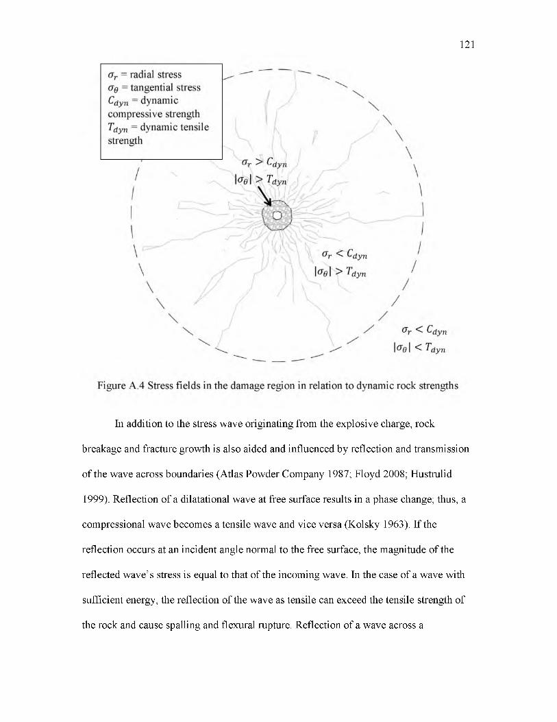
121

In addition to the stress wave originating from the explosive charge, rock

breakage and fracture growth is also aided and influenced by reflection and transmission

of the wave across boundaries (Atlas Powder Company 1987; Floyd 2008; Hustrulid

1999). Reflection of a dilatational wave at free surface results in a phase change; thus, a

compressional wave becomes a tensile wave and vice versa (Kolsky 1963). If the

reflection occurs at an incident angle normal to the free surface, the magnitude of the

reflected wave’s stress is equal to that of the incoming wave. In the case of a wave with

sufficient energy, the reflection of the wave as tensile can exceed the tensile strength of

the rock and cause spalling and flexural rupture. Reflection of a wave across a

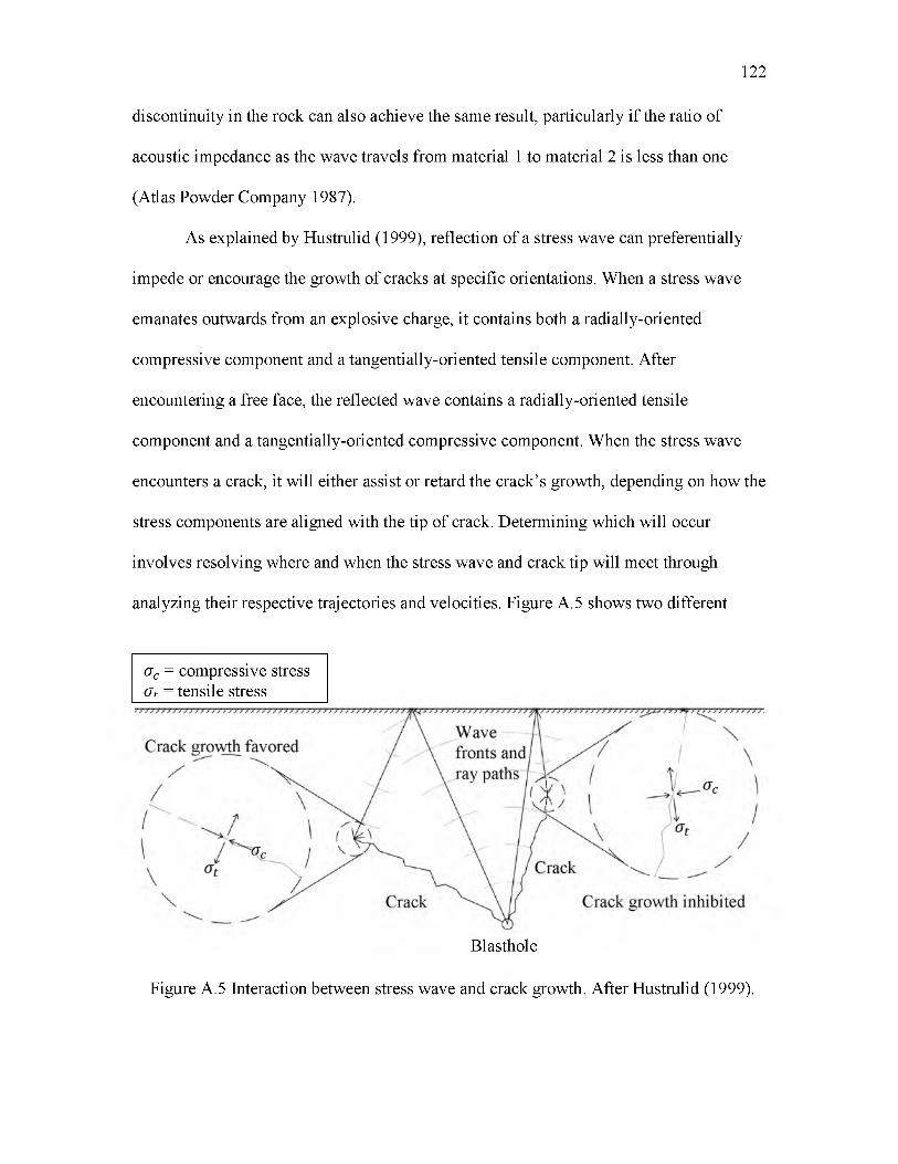
discontinuity in the rock can also achieve the same result, particularly if the ratio of

acoustic impedance as the wave travels from material 1 to material 2 is less than one

(Atlas Powder Company 1987).

As explained by Hustrulid (1999), reflection of a stress wave can preferentially

impede or encourage the growth of cracks at specific orientations. When a stress wave

emanates outwards from an explosive charge, it contains both a radially-oriented

compressive component and a tangentially-oriented tensile component. After

encountering a free face, the reflected wave contains a radially-oriented tensile

component and a tangentially-oriented compressive component. When the stress wave

encounters a crack, it will either assist or retard the crack’s growth, depending on how the

stress components are aligned with the tip of crack. Determining which will occur

involves resolving where and when the stress wave and crack tip will meet through

analyzing their respective trajectories and velocities. Figure A.5 shows two different

122

oc = compressive stress ov = tensile stress

Blasthole

Figure A.5 Interaction between stress wave and crack growth. After Hustrulid (1999).

possibilities. The scenario on the left favors crack growth while the scenario on the right

inhibits crack growth.

Initially the shock wave is travelling faster than the dilatational wave velocity cP

(ISEE 2011). The shock wave dissipates energy quickly and becomes a compressional

wave travelling at the velocity . The theoretical maximum crack tip velocity, on the

other hand, is equal to , although experiments with concrete by Curbach and Eibl

(1990) indicated actual peak velocities between 0 . 2 0 cP and 0 . 3 0 cP.

Studies into the nature of crack growth have shown that preexisting flaws and

discontinuities in a rock mass exert significant influence on the nature of the fracture

network that is formed as the stress wave passes through (Atlas Powder Company 1987).

Tests in unflawed material result in only a small number of dominant cracks that extend

far out from the borehole. The dense fracturing, and consequently the zone of

fragmentation, remains clustered near the blasthole. On the other hand, even a small flaw

some distance out from the blasthole can alter the pattern of fractures developed in that

the flaw may act as a nucleus for crack growth. Virtually all rock bodies are

heterogeneous and contain a high concentration of fractures and flaws ranging from

microscopic to macroscopic in size. Consequently, the size and shape of the

fragmentation zone from a blast is highly dependent upon the rock structure.

Beyond the fracture zone, the stress wave energies have dissipated to the point

where no further breakage occurs. These waves continue outward as elastic waves and

cause vibrations that are measurable for large distances.

123

A.3 High pressure gas expansion

Immediately after the shock wave is transmitted to the rock mass, the high

pressure gases in the expanding borehole cavity begin to force their way into the fracture

network. The gases travel along paths that offer the least resistance, which include both

the fracture network and preexisting discontinuities, cracks, faults, joints, and seams of

weak material (Atlas Powder Company 1987). Where no path exists, gas pressures may

be high enough to create new cracks or extend existing ones (Floyd 2008). The gases

continue to work within the rock matrix until either they vent at a free face or the

pressure magnitude drops to a certain threshold. Studies indicate this threshold to be

around 100 MPa (14,500 psi) (McKenzie 1999). As the gas flows out of the rock mass,

the pressure load is released (Atlas Powder Company 1987). Rebound of the rock

material instigates high tensile stresses that contribute to the breakage process.

The exact degree to which the high pressure gases contribute to the fracturing and

rupture of the rock mass has not been fully agreed upon (Atlas Powder Company 1987).

Some claim that the fracture network is complete by the time the gases begin streaming

into the rock surrounding the blasthole, while others say that a significant portion of the

fracturing is directly attributed to gas action. In all reality, the most plausible scenario is

that the shock wave and gas pressures work in conjunction with each other. One

mechanism may dominate the other, but this likely is dependent upon the structure and

properties of the in-situ rock and the properties of the explosive used. A series of

experiments were conducted by Brinkmann (1990) in which steel liners were positioned

along the blasthole walls to prevent the flow of explosive gases into the surrounding rock.

A comparison made between the normal and lined blastholes indicated that (1) the shock

124

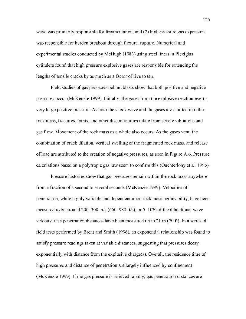
wave was primarily responsible for fragmentation, and (2) high-pressure gas expansion

was responsible for burden breakout through flexural rupture. Numerical and

experimental studies conducted by McHugh (1983) using steel liners in Plexiglas

cylinders found that high pressure explosive gases are responsible for extending the

lengths of tensile cracks by as much as a factor of five to ten.

Field studies of gas pressures behind blasts show that both positive and negative

pressures occur (McKenzie 1999). Initially, the gases from the explosive reaction exert a

very large positive pressure. As both the shock wave and the gases are emitted into the

rock mass, fractures, joints, and other discontinuities dilate from severe vibrations and

gas flow. Movement of the rock mass as a whole also occurs. As the gases vent, the

combination of crack dilation, vertical swelling of the fragmented rock mass, and release

of load are attributed to the creation of negative pressures, as seen in Figure A.6. Pressure

calculations based on a polytropic gas law seem to confirm this (Ouchterlony et al. 1996).

Pressure histories show that gas pressures remain within the rock mass anywhere

from a fraction of a second to several seconds (McKenzie 1999). Velocities of

penetration, while highly variable and dependent upon rock mass permeability, have been

measured to be around 200-300 m/s (660-980 ft/s), or 5-10% of the dilatational wave

velocity. Gas penetration distances have been measured up to 21 m (70 ft). In a series of

field tests performed by Brent and Smith (1996), an exponential relationship was found to

satisfy pressure readings taken at variable distances, suggesting that pressures decay

exponentially with distance from the explosive charge(s). Overall, the residence time of

high pressures and distance of penetration are largely influenced by confinement

(McKenzie 1999). If the gas pressure is relieved rapidly, gas penetration distances are

125

126

Figure A.6 Example pressure histories behind a bench blast (Source: McKenzie 1999. Reprinted with the permission of The Australasian Institute of

Mining and Metallurgy).

small. If an explosive charge is highly confined, peak pressures are higher, penetration

distances increase, and the pressures themselves tend to remain positive. Confinement is

controlled primarily by the effective burden between an explosive charge and free face,

but is also influenced by stemming and rock permeability.

A.4 Displacement of fragmented rock

The last stage in the fragmentation process constitutes movement of the

preconditioned rock. Both the shock/strain wave and gas pressures contribute to

displacement of the broken rock, but it is primarily gas action that is responsible for the

heave (Floyd 2008). It is at this stage that having an adequate free face is essential. Stress

relief is provided as the broken rock moves along the path of least resistance. Regions of

rock that may not have been fully fragmented experience flexural rupture from the

pressurized gas flow, provided that a free surface is present. In-air collisions of rock

fragments also add to the breakage process in a minor role (Atlas Powder Company 1987;

Floyd 2008).

A.5 Partitioning of explosive energy

Several studies have been conducted on explosive energy distribution among each

of the breakage mechanisms previously discussed (Hinzen 1998; Ouchterlony et al. 2004;

Sanchidrian et al. 2007; Spathis 1999). The results of one such study by Ouchterlony et

al. (2004) are presented here. The following energy balance was used in partitioning the

energy:

t]E0 = Ek + Ef + Es + other Iosses (A.6)

where

E0 is the explosive weight strength,

Ek is the kinetic energy of throw,

Ef is the fragmentation energy (based on the creation of new surface area through

fracturing),

Es is seismic energy,

rj = EG / E0 is the utilization ratio or relative work capacity of the explosive, where EG is

called the Gurney energy determined using the cylinder expansion tests, and

127

o ther Iosses include a number of factors: heat transferred to the rock mass, shock wave

losses such as crushing, friction losses, etc.

Losses included in the term are residual heat from blast fumes, air shock waves,

and sometimes an incomplete chemical reaction of the explosive. Usable work from the

explosive is contained in the kinetic energy and fragmentation terms. The results of the

study were as follows:

• Crushing and other losses in the rock mass 20-40%,

• Kinetic energy of throw 10-20%,

• Seismic energy 5-10%, and

• Fragmentation energy 0.1-2%.

These are only rough estimates. However, they give one an overall idea of the

energy content of each breakage mechanism.

A.6 Fracture mechanics

The field of fracture mechanics is quite extensive and complex in nature. While

little attention will be given in this thesis to a rigorous study of fractures, its strong

presence in the fragmentation process requires that it at least be mentioned.

Cracks form in brittle materials as a result of failure either through compression,

shear, or tension. Depending on the conditions of failure, the latter two tend to be more

common as the stress magnitudes at failure in shear and tension are lower than in

compression. As pointed out by Persson et al. (1994), the relative energies of deformation

until fracture in uniaxial tension versus uniaxial compression are 1:100. Once a crack is

formed, further brittle failure is directed in a manner that extends crack growth. This

growth results from tensile stresses that concentrate at the tip of the crack.

128

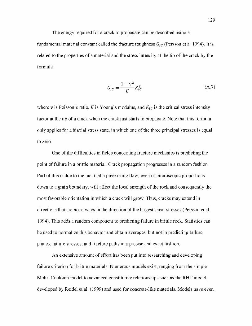
The energy required for a crack to propagate can be described using a

fundamental material constant called the fracture toughness (Persson et al 1994). It is

related to the properties of a material and the stress intensity at the tip of the crack by the

formula

G , c = ^ f - K f c (A 7)

where v is Poisson’s ratio, E is Young’s modulus, and KIC is the critical stress intensity

factor at the tip of a crack when the crack just starts to propagate. Note that this formula

only applies for a biaxial stress state, in which one of the three principal stresses is equal

to zero.

One of the difficulties in fields concerning fracture mechanics is predicting the

point of failure in a brittle material. Crack propagation progresses in a random fashion.

Part of this is due to the fact that a preexisting flaw, even of microscopic proportions

down to a grain boundary, will affect the local strength of the rock and consequently the

most favorable orientation in which a crack will grow. Thus, cracks may extend in

directions that are not always in the direction of the largest shear stresses (Persson et al.

1994). This adds a random component to predicting failure in brittle rock. Statistics can

be used to normalize this behavior and obtain averages, but not in predicting failure

planes, failure stresses, and fracture paths in a precise and exact fashion.

An extensive amount of effort has been put into researching and developing

failure criterion for brittle materials. Numerous models exist, ranging from the simple

Mohr-Coulomb model to advanced constitutive relationships such as the RHT model,

developed by Reidel et al. (1999) and used for concrete-like materials. Models have even

129

been developed specifically for estimating blast damage, such as Yang et al. (1996) and

Yang and Wang (1996). One of the more interesting theories on brittle failure was

developed by Lundborg (1972). His theory uses a random microcrack model to formulate

a statistical theory of brittle material strength. When simplified, however, this theory can

be reduced down to the classical models of Mohr-Coulomb, von Mises, Tresca, and

others (Persson et al. 1994).

A.7 Blasting to minimize damage

Blast-induced damage manifests itself in a number of forms during blasting

operations. These may include the following (Floyd 2008):

• Compressional failure surrounding each blasthole;

• Tensile failure in the form of spalling and radial fractures;

• Shear failure and slippage, particularly along preexisting planes;

• Crack extension through both tensile failure and gas penetration;

• Block heaving and cratering behind a blast from high gas pressures; and

• Release of load fracturing from the rebounding rock mass.

Various field techniques have been developed for minimizing backbreak. These

range from simple modifications on production blasts to specialized blast designs that

require additional effort to implement. The five main types according to Floyd (2008) and

Oriard (1972, 1982) are explained as follows.

A.7.1 Modified production or trim blast

In this type of blast, one or more design parameters are changed such as the

number of rows, delay sequence, etc. (Floyd 2008). Often, the number of rows is limited,

130

providing a narrow pattern width in which effective burden control (i.e., adequate free

face) can be assured. This type of blast is most easily implemented without hindering

production operations.

A.7.2 Cushion or buffer blast

A cushion or buffer blast is similar to a trim blast, but the last row or two have

smaller charge weights, reduced burden and spacing, and little or no stemming (Floyd

2008). Narrow blasts of three or four rows are conducted. Care is taken to ensure that

adequate horizontal relief is provided as each row is detonated in succession.

A.7.3 Presplit or midsplit blasting

Presplitting involves drilling a row of closely-spaced holes at the pattern design

limits and detonating them prior to the adjacent rows (Floyd 2008; Oriard 1982). The

objective is to create a fracture line that will impede the penetration of high-pressure

gases into the bench and limit crack growth. By using decoupled or light charges with no

stemming, the shock wave applied by the borehole pressure is minimized (Oriard 1982).

As the expanding gases apply a less damaging pressure pulse on the borehole walls, a

quasistatic stress field is created that favors the formation of a tensile crack between

presplit holes, as displayed in Figure A.7. If the fracture extends the entire distance

between adjacent holes, a pathway is made for gases from blasting to vent out the surface

instead of penetrating into the rock beyond the intended limit. In order for a presplit to be

successful, though, adjacent holes must be detonated simultaneously to create the

appropriate stresses. One caveat with presplitting is that additional, unintended damage

may be induced (Oriard 1982). Drilling accuracy is also critical in creating an effective

131

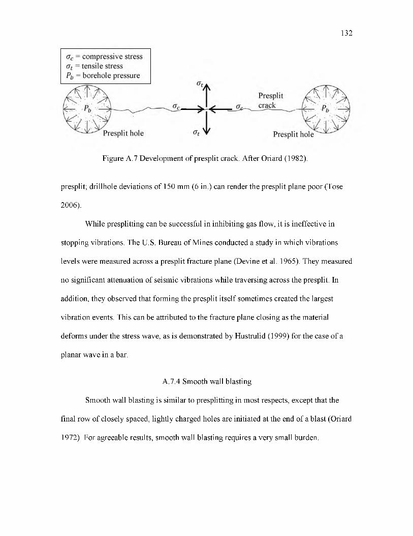
132

Figure A.7 Development of presplit crack. After Oriard (1982).

presplit; drillhole deviations of 150 mm (6 in.) can render the presplit plane poor (Tose

2006).

While presplitting can be successful in inhibiting gas flow, it is ineffective in

stopping vibrations. The U.S. Bureau of Mines conducted a study in which vibrations

levels were measured across a presplit fracture plane (Devine et al. 1965). They measured

no significant attenuation of seismic vibrations while traversing across the presplit. In

addition, they observed that forming the presplit itself sometimes created the largest

vibration events. This can be attributed to the fracture plane closing as the material

deforms under the stress wave, as is demonstrated by Hustrulid (1999) for the case of a

planar wave in a bar.

A.7.4 Smooth wall blasting

Smooth wall blasting is similar to presplitting in most respects, except that the

final row of closely spaced, lightly charged holes are initiated at the end of a blast (Oriard

1972). For agreeable results, smooth wall blasting requires a very small burden.

A.7.5 Line drilling

When a smooth wall with no out-of-plane fracturing or damage is essential, line

drilling can be used. A line of holes spaced closely at 6- to 12-hole diameters apart is

drilled along the final wall. No explosive is loaded in these holes. A buffer row is drilled

adjacent to the line with reduced spacing and loaded with a light charge.

133

APPENDIX B

WAVE PROPAGATION AND SEISMIC

VIBRATIONS

As discussed in Section A.5 in Appendix A, the detonation of an explosive charge

in rock transmits a large amount of energy to its surroundings in a very short timeframe.

Around 5-10% of this energy results in seismic disturbances (Ouchterlony et al. 2004).

Although seemingly small, this portion of the energy released plays a significant role

both in extending the outer fringes of the fracture zone and in affecting the stability of

slopes, excavations, and structures at further distances.

Numerous studies have been conducted into studying blast-induced waves and

how to minimize the vibrations they generate. Blast vibrations may be divided into near­

field and far-field. The distinction lies in the types of waves that occur. Near-field

vibrations concern close distances on the order of 15 m (50 ft), in which body waves are

predominant. Far-field vibrations are dominated by surface waves and can be perceived

for thousands of feet. Most vibration analyses focus on far-field effects, for these are a

greater cause for concern among mining operations and construction activities. Rock

damage, however, is influenced by near-field vibrations. Whatever the emphasis, a key

component to studying blast-induced damage lies in understanding the fundamentals of

seismic waves.

B.1 Fundamentals of seismic waves

In a basic sense, physical waves are the propagation of energy through a medium.

Most waves can be approximated as elastic. This allows for the simplifications that

permit development of the formal mathematical theory and provides a starting point for

understanding nonelastic wave behavior. A propagating wave exhibits certain distinct

characteristics. A wave propagates by transferring the energy disturbance from one

element in the elastic continuum to the next through the action of forces (Bollinger 1971).

135

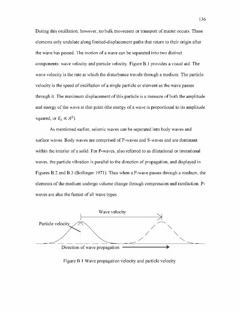
During this oscillation, however, no bulk movement or transport of matter occurs. These

elements only undulate along limited-displacement paths that return to their origin after

the wave has passed. The motion of a wave can be separated into two distinct

components: wave velocity and particle velocity. Figure B.1 provides a visual aid. The

wave velocity is the rate at which the disturbance travels through a medium. The particle

velocity is the speed of oscillation of a single particle or element as the wave passes

through it. The maximum displacement of this particle is a measure of both the amplitude

and energy of the wave at that point (the energy of a wave is proportional to its amplitude

squared, or ).

As mentioned earlier, seismic waves can be separated into body waves and

surface waves. Body waves are comprised of P-waves and S-waves and are dominant

within the interior of a solid. For P-waves, also referred to as dilatational or irrotational

waves, the particle vibration is parallel to the direction of propagation, and displayed in

Figures B.2 and B.3 (Bollinger 1971). Thus when a P-wave passes through a medium, the

elements of the medium undergo volume change through compression and rarefaction. P-

waves are also the fastest of all wave types.

136

Wave velocity----------------- y--------------------->1

Figure B.1 Wave propagation velocity and particle velocity

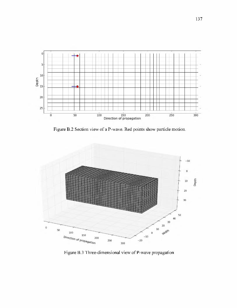
Dep

th

137

Figure B.2 Section view of a P-wave. Red points show particle motion.

Figure B.3 Three-dimensional view of P-wave propagation

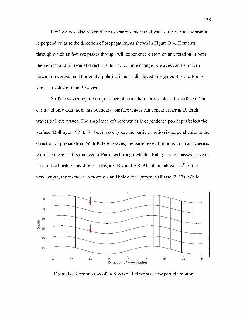
For S-waves, also referred to as shear or distortional waves, the particle vibration

is perpendicular to the direction of propagation, as shown in Figure B.4. Elements

through which an S-wave passes through will experience distortion and rotation in both

the vertical and horizontal directions, but no volume change. S-waves can be broken

down into vertical and horizontal polarizations, as displayed in Figures B.5 and B.6. S-

waves are slower than P-waves.

Surface waves require the presence of a free boundary such as the surface of the

earth and only exist near this boundary. Surface waves can appear either as Raleigh

waves or Love waves. The amplitude of these waves is dependent upon depth below the

surface (Bollinger 1971). For both wave types, the particle motion is perpendicular to the

direction of propagation. With Raleigh waves, the particle oscillation is vertical, whereas

with Love waves it is transverse. Particles through which a Raleigh wave passes move in

an elliptical fashion, as shown in Figures B.7 and B.8. At a depth above 1/5th of the

wavelength, the motion is retrograde, and below it is prograde (Russel 2013). While

138

0 10 20 30 40 50 60 70 80Direction of propagation

Figure B.4 Section view of an S-wave. Red points show particle motion.

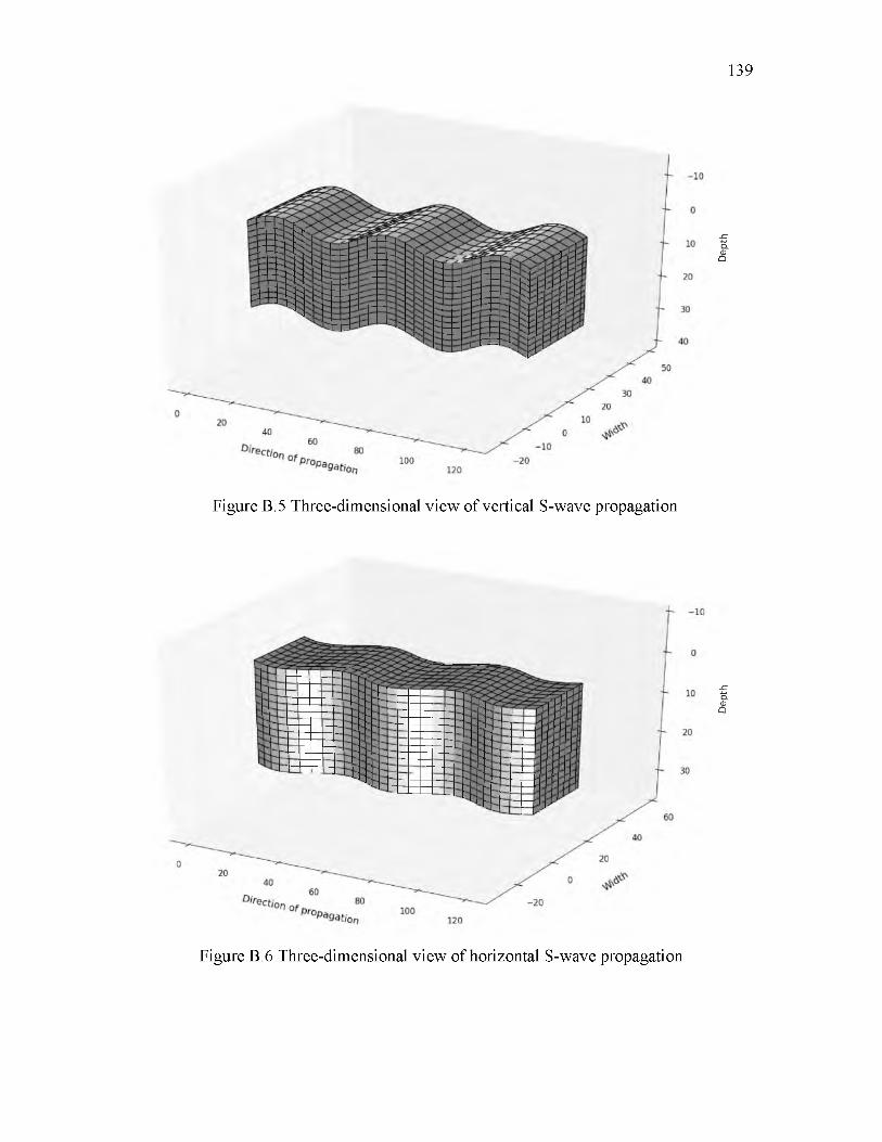
139

Figure B.5 Three-dimensional view of vertical S-wave propagation

Figure B.6 Three-dimensional view of horizontal S-wave propagation

Dept

h D

epth

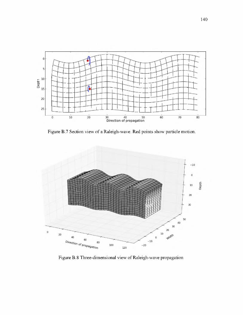
Dep

th

140

Figure B.7 Section view of a Raleigh-wave. Red points show particle motion.

Figure B.8 Three-dimensional view of Raleigh-wave propagation

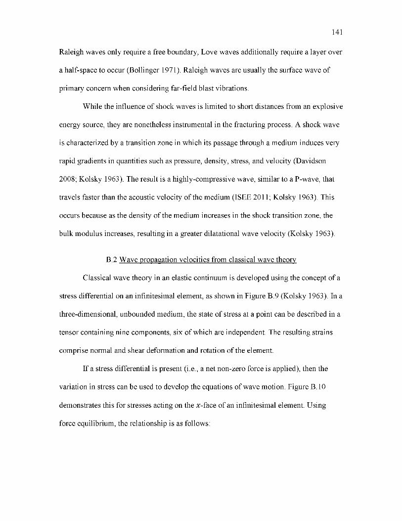
Raleigh waves only require a free boundary, Love waves additionally require a layer over

a half-space to occur (Bollinger 1971). Raleigh waves are usually the surface wave of

primary concern when considering far-field blast vibrations.

While the influence of shock waves is limited to short distances from an explosive

energy source, they are nonetheless instrumental in the fracturing process. A shock wave

is characterized by a transition zone in which its passage through a medium induces very

rapid gradients in quantities such as pressure, density, stress, and velocity (Davidson

2008; Kolsky 1963). The result is a highly-compressive wave, similar to a P-wave, that

travels faster than the acoustic velocity of the medium (ISEE 2011; Kolsky 1963). This

occurs because as the density of the medium increases in the shock transition zone, the

bulk modulus increases, resulting in a greater dilatational wave velocity (Kolsky 1963).

B.2 Wave propagation velocities from classical wave theory

Classical wave theory in an elastic continuum is developed using the concept of a

stress differential on an infinitesimal element, as shown in Figure B.9 (Kolsky 1963). In a

three-dimensional, unbounded medium, the state of stress at a point can be described in a

tensor containing nine components, six of which are independent. The resulting strains

comprise normal and shear deformation and rotation of the element.

If a stress differential is present (i.e., a net non-zero force is applied), then the

variation in stress can be used to develop the equations of wave motion. Figure B.10

demonstrates this for stresses acting on the x-face of an infinitesimal element. Using

force equilibrium, the relationship is as follows:

141

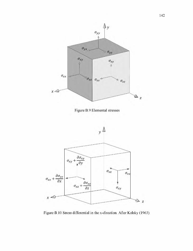
142

Figure B.10 Stress differential in the x-direction. After Kolsky (1963).

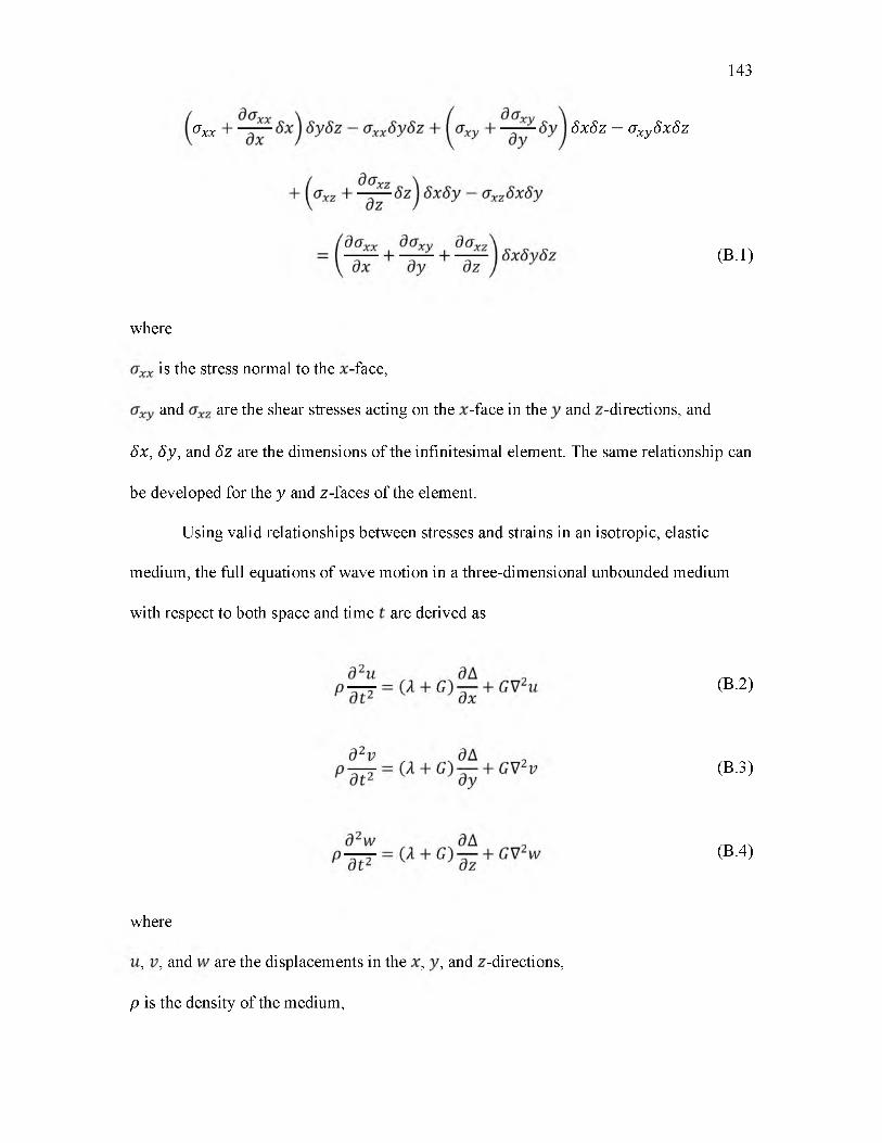
143

®xx SxSz — aXy5x5z

(B.1)

where

is the stress normal to the -face,

and are the shear stresses acting on the -face in the and -directions, and

Sx, Sy, and Sz are the dimensions of the infinitesimal element. The same relationship can

be developed for the y and z-faces of the element.

Using valid relationships between stresses and strains in an isotropic, elastic

medium, the full equations of wave motion in a three-dimensional unbounded medium

with respect to both space and time are derived as

(B.2)

(B.3)

(B.4)

where

, , and are the displacements in the , , and -directions,

p is the density of the medium,

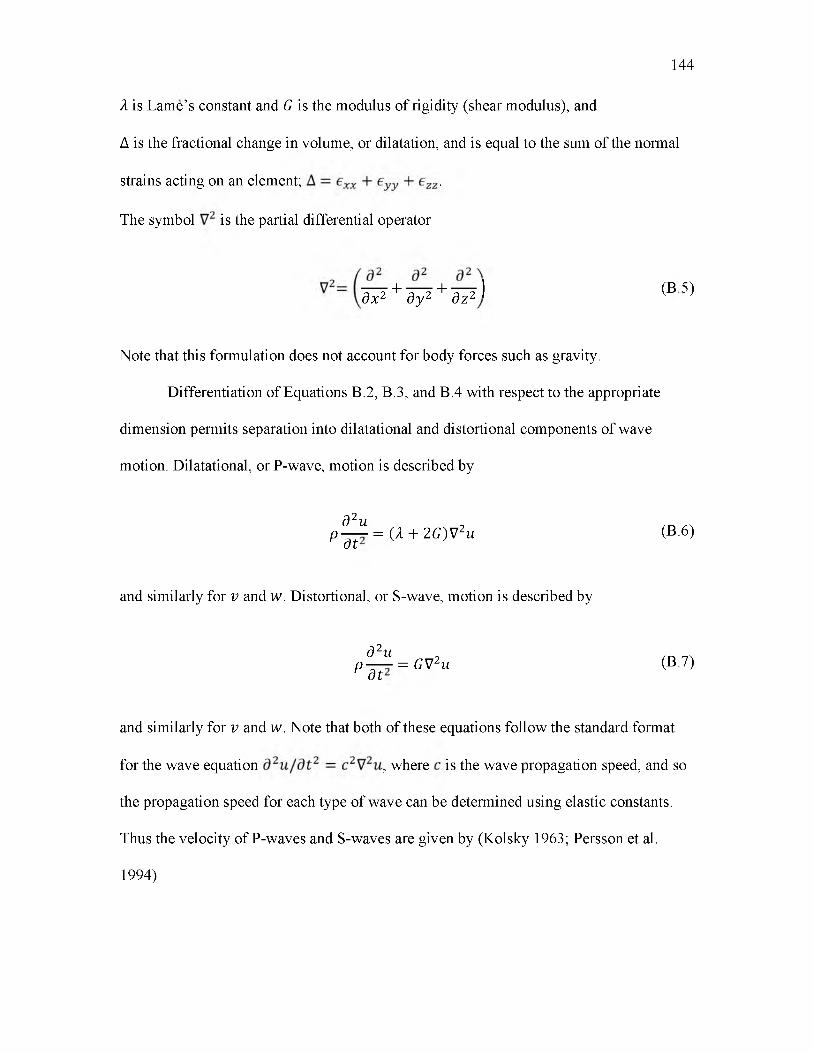
A is Lame’s constant and G is the modulus of rigidity (shear modulus), and

A is the fractional change in volume, or dilatation, and is equal to the sum of the normal

strains acting on an element; .

The symbol is the partial differential operator

144

+ ^TT7 + TT?) (B 5)dx2 d y 2 d z 2

Note that this formulation does not account for body forces such as gravity.

Differentiation of Equations B.2, B.3, and B.4 with respect to the appropriate

dimension permits separation into dilatational and distortional components of wave

motion. Dilatational, or P-wave, motion is described by

d 2u _ _p — = (A + 2 G)V2u (B.6)

dt

and similarly for v and w. Distortional, or S-wave, motion is described by

P ^ U = GV2u (B.7)o t

and similarly for v and w. Note that both of these equations follow the standard format

for the wave equation , where is the wave propagation speed, and so

the propagation speed for each type of wave can be determined using elastic constants.

Thus the velocity of P-waves and S-waves are given by (Kolsky 1963; Persson et al.

1994)

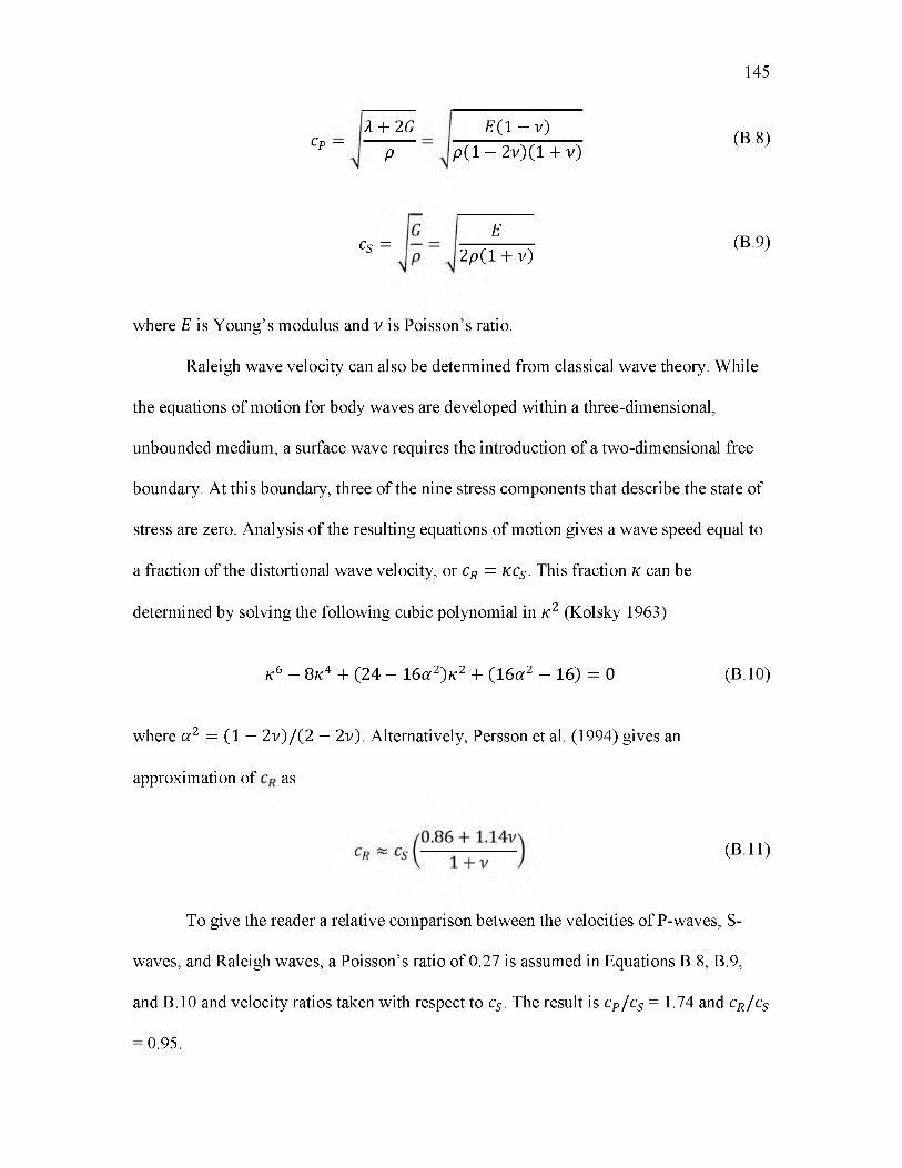
145

A + 2G E( 1 —v ) (B.8)cP —P p ( 1 — 2v)( 1 + v)

Cs = 2p ( 1 + v)E

(B 9)

where E is Young’s modulus and v is Poisson’s ratio.

Raleigh wave velocity can also be determined from classical wave theory. While

the equations of motion for body waves are developed within a three-dimensional,

unbounded medium, a surface wave requires the introduction of a two-dimensional free

boundary. At this boundary, three of the nine stress components that describe the state of

stress are zero. Analysis of the resulting equations of motion gives a wave speed equal to

a fraction of the distortional wave velocity, or c R = kcs . This fraction k can be

determined by solving the following cubic polynomial in k 2 (Kolsky 1963)

To give the reader a relative comparison between the velocities of P-waves, S-

waves, and Raleigh waves, a Poisson’s ratio of 0.27 is assumed in Equations B.8, B.9,

and B.10 and velocity ratios taken with respect to cs . The result is cP/ cs = 1.74 and cR/c s

k6 — 8 k4 + ( 2 4 — 16 a 2)K2 + ( 16 a 2 — 16) = 0 (B.10)

where a 2 = (1 — 2 v ) / ( 2 — 2v). Alternatively, Persson et al. (1994) gives an

approximation of as

(B11)

0.95.

B.3 Attenuation of wave energy

All seismic waves travelling through a medium, even ideal ones in which no

energy is absorbed through friction losses, experience a decrease in amplitude as they

progress. This is called attenuation. The only exception to this is an ideal plane wave

travelling through a bar. Hustrulid (1999) identified four primary causes of attenuation:

• Geometric spreading - The decrease in amplitude that occurs as a

wavefront encompasses an ever-increasing region. Energy is not lost, just

spread over a larger region. The amplitude reduction can be calculated as

146

A = — (B.12)fin v 7

where A is the amplitude of the wave at a distance R from its energy

source, is the original amplitude, and is a constant equal to 0 for

plane waves, 1/2 for cylindrical waves, and 1 for spherical waves

(Hustrulid 1999).

• Dispersion - Dispersion refers to the broadening of a wave pulse as its

constitutive frequency components travel at different rates. In a perfectly-

elastic, isotropic medium, a wave will not disperse. However, a number of

factors such as variations in a material’s elastic properties, discontinuities

and boundaries, internal friction, anisotropy, etc., will cause the velocities

of the components of a wave to become frequency dependent (Bollinger

1971; Hustrulid 1999; Kolsky 1963). Usually, the high frequency

components travel at slower speeds than the low frequency components

(Hustrulid 1999). As different frequency-velocity groups separate, the

147

result is a “spreading” of a wave and a reduction in amplitude and thus

energy.

• Reflection at acoustic boundaries - When a wave meets an internal

boundary, a portion of it is reflected, and thus energy is retained in the

system that would have originally continued onwards. As can be

imagined, a typical body of rock contains numerous internal boundaries

ranging from grain-sized to large discontinuities and thus, attenuation

through internal reflections is present.

• Damping - Damping, also called inelastic attenuation, occurs as a result of

internal friction losses when energy is absorbed from the wave by the

medium.

Attenuation can be simplistically modeled using two different approaches: an

exponential law and a power law (Hustrulid 1999). They are

where and are attenuation factors that incorporate the four sources of attenuation as

previously discussed. Both approaches have been used in technical studies with success.

Hustrulid (1999) makes the claim that the exponential law appears to be the most

technically apt formulation for studying attenuation. He does note, though, that the power

law has provided a stronger statistical correlation with experimental data in some studies.

A = A 0e~aR (B13)

(B14)

148

One widely used approach to estimating seismic attenuation is through the use of

the seismic quality factor Q, first pioneered by Born (1941). Studies of wave attenuation

in rock samples of varying quality have shown that over a large range of frequencies, the

energy losses of a wave can be described using a factor specific to the rock quality. The

underlying relationship is

AEt 2n

where is the energy contained in a wave at cycle , is the wave energy lost per

cycle i, and Q is the seismic quality factor specific to the rock type (Hustrulid 1999).

Over cycles, the energy content is given by

where is the energy initially contained in the wave and is the energy available in

the wave after n cycles. When using the exponential law presented in Equation B.13 and

where is the wavelength of a specific frequency component of a seismic wave.

Since higher frequency wave components oscillate much more rapidly within a

given travel distance than low frequency wave components, the end result is that high

frequencies within a wave will attenuate much more rapidly. As noted by Born (1941),

the ground acts as a low-pass filter. In the context of rock blasting, the implication is that

(B.16)

noting that for a wave , the Q factor can by incorporated as

A = A 0e aR = A 0eQx (B.17)

blast-induced seismic vibrations will increasingly shift towards containing low dominant

frequencies as they travel farther away from the explosive energy source. Kjartansson

(1979) developed a transfer function for Q-based attenuation that can easily be applied in

the frequency domain. Several individuals have used Kjartansson’s work to incorporate

the Q factor into blast vibration attenuation models (Blair and Spathis 1982; Yang and

Scovira 2010).

It is worth noting that while the Q factor seems to work quite well, there are

instances where it can be inadequate (Hustrulid 1999). Also, conservation of momentum

is not preserved using Q-based attenuation. As the radius of the wave front increases, the

net momentum of the wave decreases. This is the result of assuming a constant wave

propagation velocity.

B.4 Blasting vibrations

A significant amount of time and effort has been dedicated in the mining industry

to understanding and controlling blast-induced ground vibrations. Most studies have

focused on the effects of far-field surface vibrations and their effects on structures, with

some of the most extensive ones being conducted by the U.S. Bureau of Mines. As

mentioned at the beginning of the chapter, blast vibrations can be categorized into two

types: near-field and far-field. The delineator lies in the types of waves encountered at

different distances from the energy source. Within the immediate region of the explosive

charge, the majority of seismic motion occurs as body waves emanating from the blast.

Further out, a portion of these become surface waves as they encounter the surface of the

ground. Since surface waves are confined to the plane of the earth’s surface, their energy

does not spread as rapidly as body waves. Thus, body waves are predominant in the near­

149

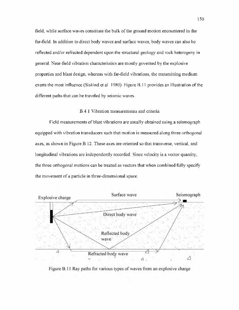
field, while surface waves constitute the bulk of the ground motion encountered in the

far-field. In addition to direct body waves and surface waves, body waves can also be

reflected and/or refracted dependent upon the structural geology and rock heterogeny in

general. Near-field vibration characteristics are mostly governed by the explosive

properties and blast design, whereas with far-field vibrations, the transmitting medium

exerts the most influence (Siskind et al. 1980). Figure B.11 provides an illustration of the

different paths that can be traveled by seismic waves.

B.4.1 Vibration measurements and criteria

Field measurements of blast vibrations are usually obtained using a seismograph

equipped with vibration transducers such that motion is measured along three orthogonal

axes, as shown in Figure B.12. These axes are oriented so that transverse, vertical, and

longitudinal vibrations are independently recorded. Since velocity is a vector quantity,

the three orthogonal motions can be treated as vectors that when combined fully specify

the movement of a particle in three-dimensional space.

150

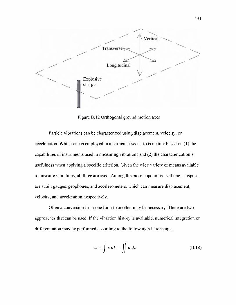
151

^ Explosive ,charge ... 'r

Figure B.12 Orthogonal ground motion axes

Particle vibrations can be characterized using displacement, velocity, or

acceleration. Which one is employed in a particular scenario is mainly based on (1) the

capabilities of instruments used in measuring vibrations and (2) the characterization’s

usefulness when applying a specific criterion. Given the wide variety of means available

to measure vibrations, all three are used. Among the more popular tools at one’s disposal

are strain gauges, geophones, and accelerometers, which can measure displacement,

velocity, and acceleration, respectively.

Often a conversion from one form to another may be necessary. There are two

approaches that can be used. If the vibration history is available, numerical integration or

differentiation may be performed according to the following relationships.

u = j v d t = J a d t (B18)

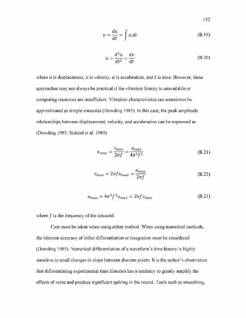
152

du f ,v - — - I a d t (B.19)

a t J

a = d l = d . (B.20)d t 2 d t

where u is displacement, v is velocity, a is acceleration, and t is time. However, these

approaches may not always be practical if the vibration history is unavailable or

computing resources are insufficient. Vibration characteristics can sometimes be

approximated as simple sinusoids (Dowding 1985). In this case, the peak amplitude

relationships between displacement, velocity, and acceleration can be expressed as

(Dowding 1985; Siskind et al. 1980)

ymax umax _Um a x - ^ J - - ^ T j 2 (B21)

o r maxvmax — 2 TC f umax — (B.22)

Q-max ~ 4/r f Umax — 2 T f Vmax (B23)

where is the frequency of the sinusoid.

Care must be taken when using either method. When using numerical methods,

the inherent accuracy of either differentiation or integration must be considered

(Dowding 1985). Numerical differentiation of a waveform’s time history is highly

sensitive to small changes in slope between discrete points. It is the author’s observation

that differentiating experimental time histories has a tendency to greatly amplify the

effects of noise and produce significant spiking in the record. Tools such as smoothing,

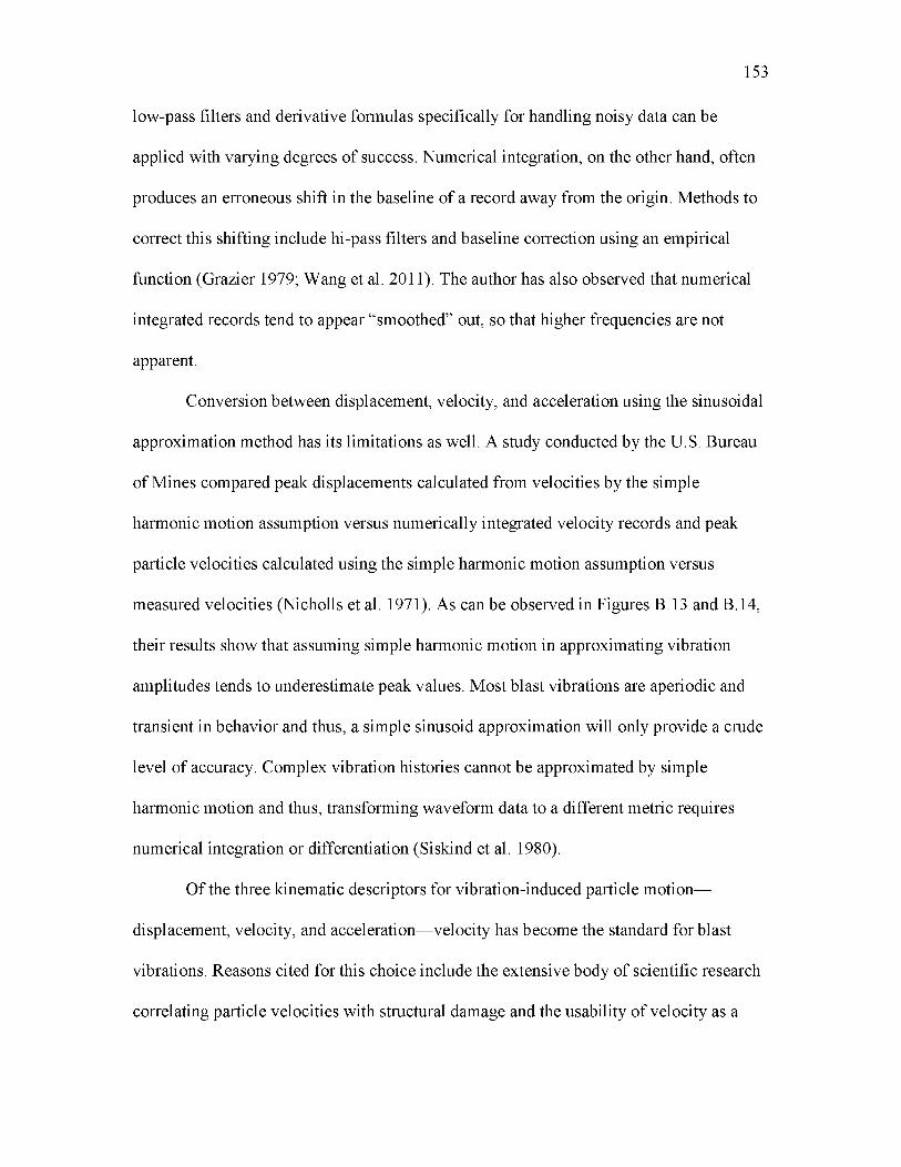
low-pass filters and derivative formulas specifically for handling noisy data can be

applied with varying degrees of success. Numerical integration, on the other hand, often

produces an erroneous shift in the baseline of a record away from the origin. Methods to

correct this shifting include hi-pass filters and baseline correction using an empirical

function (Grazier 1979; Wang et al. 2011). The author has also observed that numerical

integrated records tend to appear “smoothed” out, so that higher frequencies are not

apparent.

Conversion between displacement, velocity, and acceleration using the sinusoidal

approximation method has its limitations as well. A study conducted by the U.S. Bureau

of Mines compared peak displacements calculated from velocities by the simple

harmonic motion assumption versus numerically integrated velocity records and peak

particle velocities calculated using the simple harmonic motion assumption versus

measured velocities (Nicholls et al. 1971). As can be observed in Figures B.13 and B.14,

their results show that assuming simple harmonic motion in approximating vibration

amplitudes tends to underestimate peak values. Most blast vibrations are aperiodic and

transient in behavior and thus, a simple sinusoid approximation will only provide a crude

level of accuracy. Complex vibration histories cannot be approximated by simple

harmonic motion and thus, transforming waveform data to a different metric requires

numerical integration or differentiation (Siskind et al. 1980).

Of the three kinematic descriptors for vibration-induced particle motion—

displacement, velocity, and acceleration—velocity has become the standard for blast

vibrations. Reasons cited for this choice include the extensive body of scientific research

correlating particle velocities with structural damage and the usability of velocity as a

153

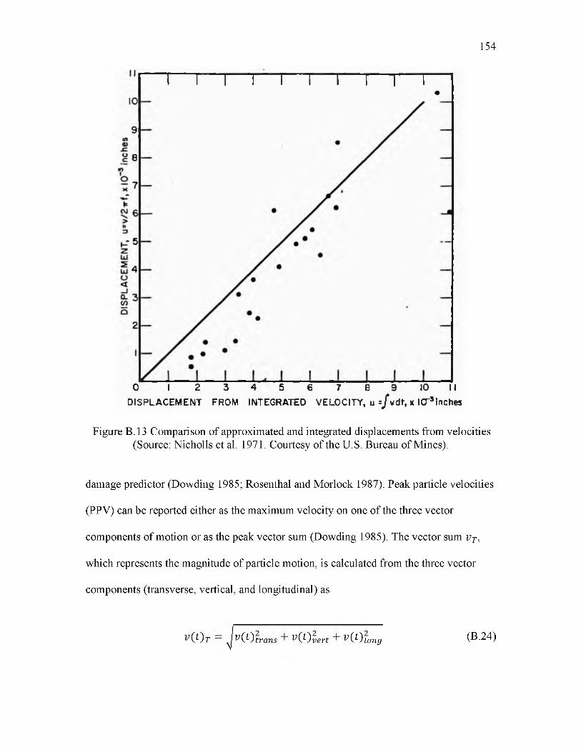
154

i— i— i— i— i— i— i— i— i— r ~m

0 I 2 3 4 5 6 7 8 9 10 II DISPLACEMENT FROM INTEGRATED VELOCITY, u = /v d t, x I0*3 inches

Figure B.13 Comparison of approximated and integrated displacements from velocities (Source: Nicholls et al. 1971. Courtesy of the U.S. Bureau of Mines).

damage predictor (Dowding 1985; Rosenthal and Morlock 1987). Peak particle velocities

(PPV) can be reported either as the maximum velocity on one of the three vector

components of motion or as the peak vector sum (Dowding 1985). The vector sum v T,

which represents the magnitude of particle motion, is calculated from the three vector

components (transverse, vertical, and longitudinal) as

v ( O t -JV( )̂t;rans v ( tyvert v (Oi ong (B.24)

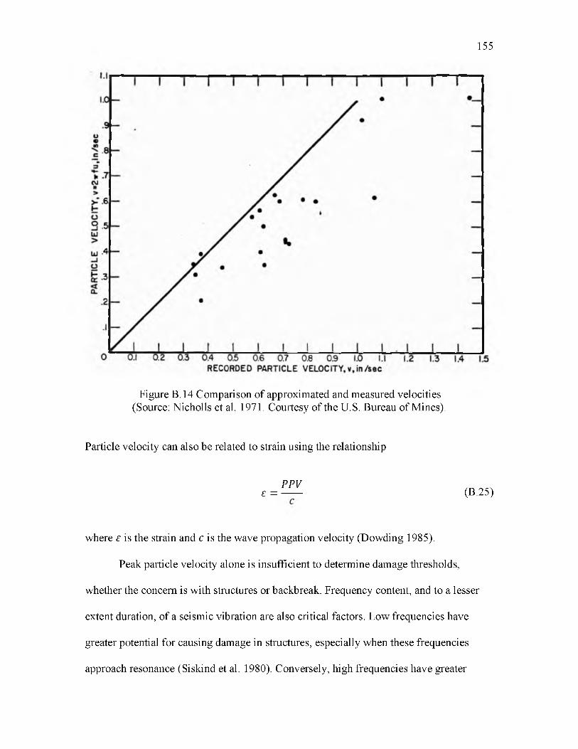
155

Figure B.14 Comparison of approximated and measured velocities (Source: Nicholls et al. 1971. Courtesy of the U.S. Bureau of Mines).

Particle velocity can also be related to strain using the relationship

PPV£ = (B.25)

where e is the strain and c is the wave propagation velocity (Dowding 1985).

Peak particle velocity alone is insufficient to determine damage thresholds,

whether the concern is with structures or backbreak. Frequency content, and to a lesser

extent duration, of a seismic vibration are also critical factors. Low frequencies have

greater potential for causing damage in structures, especially when these frequencies

approach resonance (Siskind et al. 1980). Conversely, high frequencies have greater

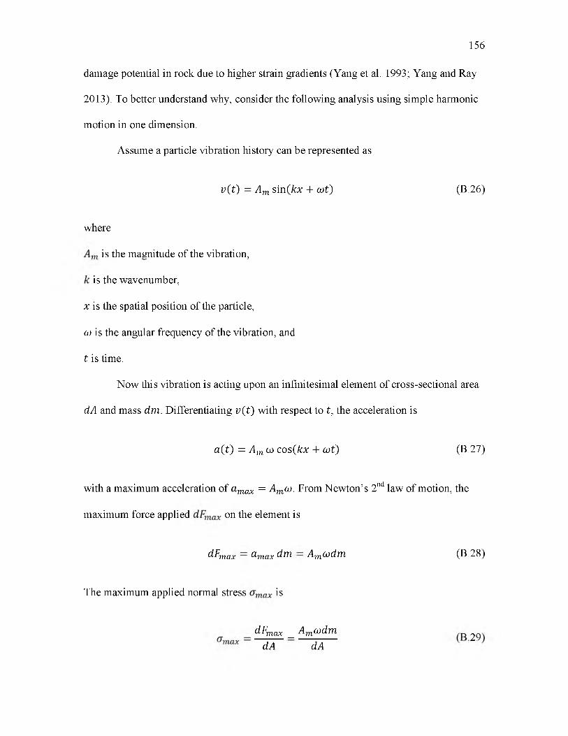
damage potential in rock due to higher strain gradients (Yang et al. 1993; Yang and Ray

2013). To better understand why, consider the following analysis using simple harmonic

motion in one dimension.

Assume a particle vibration history can be represented as

v ( t ) = Am si n( kx + o t ) (B.26)

where

is the magnitude of the vibration,

is the wavenumber,

x is the spatial position of the particle,

o is the angular frequency of the vibration, and

t is time.

Now this vibration is acting upon an infinitesimal element of cross-sectional area

dA and mass dm. Differentiating v ( t) with respect to t, the acceleration is

a ( t ) = Am o c o s( kx + o t ) (B.27)

with a maximum acceleration of amax = A mo . From Newton’s 2nd law of motion, the

maximum force applied on the element is

d ̂ max amax d m A mo d m (B.28)

The maximum applied normal stress is

156

dFmax _ Am(odm ^dA dA

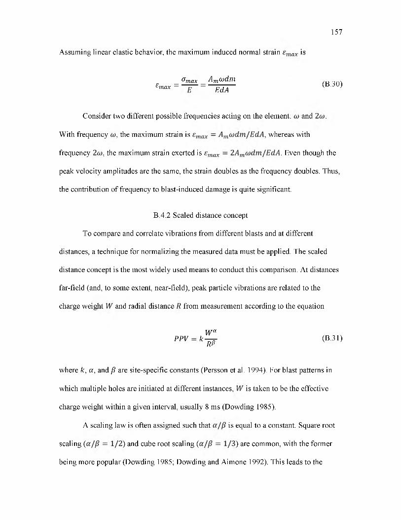
Assuming linear elastic behavior, the maximum induced normal strain is

157

@max Am(x)d,Tflw = — = - g d A - (B30)

Consider two different possible frequencies acting on the element: and .

With frequency , the maximum strain is , whereas with

frequency , the maximum strain exerted is . Even though the

peak velocity amplitudes are the same, the strain doubles as the frequency doubles. Thus,

the contribution of frequency to blast-induced damage is quite significant.

B.4.2 Scaled distance concept

To compare and correlate vibrations from different blasts and at different

distances, a technique for normalizing the measured data must be applied. The scaled

distance concept is the most widely used means to conduct this comparison. At distances

far-field (and, to some extent, near-field), peak particle vibrations are related to the

charge weight and radial distance from measurement according to the equation

W ap P V = k W (B31)

where k, a, and /? are site-specific constants (Persson et al. 1994). For blast patterns in

which multiple holes are initiated at different instances, is taken to be the effective

charge weight within a given interval, usually 8 ms (Dowding 1985).

A scaling law is often assigned such that is equal to a constant. Square root

scaling ( ) and cube root scaling ( ) are common, with the former

being more popular (Dowding 1985; Dowding and Aimone 1992). This leads to the

158

normalization of both distance and charge into what is termed “scaled distance,” as

shown in Equation B.32.

The differences in using square root versus cube root scaling lie in their origins.

In both, the vibration amplitude attenuation is assumed to be related to the ratio of the

distance from the explosive charge over the charge’s radius, or R/ re. With square root

scaling, the explosive charge is assumed to be a long cylinder (i.e., a blasthole). Since the

radius of the blasthole is proportional to the square root of the charge weight, R / r e =

R/ W 1/2. With cube root scaling, the explosive is assumed to be a spherical or point

charge. Thus, since the radius of the charge is proportional to the cube root of the charge

weight, .

There are advantages and disadvantages to both scaling laws. Only brief mention

of them is given here; for more complete discussions, see Oriard (1982) or Dowding

(1985). Square root scaling has become the prevailing tool (Dowding and Aimone 1992).

Reasons for this convention include prevalence in studies by the U.S. Bureau of Mines

and greater accuracy when predicting at farther distances (Oriard 1982). Cube root

scaling tends to be more accurate at close distances. Cube root scaling also enjoys a

theoretical backing with regards to energy considerations and is dimensionally consistent

according to the Buckingham Pi Theorem (Dowding 1985; Oriard 1982). At medium

distances, neither scaling law holds a distinct advantage.

As stated by Oriard (1982), what is important to bear in mind is that the scaled

distance concept is a means by which comparisons of vibrations generated by different

explosive charge sizes measured at different distances can be made for an expected range

of data. It is not meant to give highly-accurate predictions nor facilitate theoretical

correctness in predicting vibration attenuation. The scaled distance approach tends to fit

rather poorly over large ranges. Its efficacy at close and medium distances has also been

questioned (Blair 1987). Attempts to overcome this have been developed, ranging from

using different best fit equations for specific domains to incorporating additional

complexity.

B.4.3 Fitting a scaled distance model to field data

To determine the constants in Equation B.32, a data set with a reasonable amount

of variability is needed. Once such a set is available, the common approach to fitting a

curve is with the least squares linear regression technique. Linearization of Equation B.32

gives rise an equation of the form

\nP P V = - p i n S D + \ n k (B.33)

This is identical to the equation of a line y = m x + b. Using the least squares approach

as outlined in any statistics textbook, the best fit line is determined through minimizing

the sum of the squares of the error (see Montgomery and Runger 2007). However, as

noted by Smith (2003), applying such an approach to the scaled distance transformation

in Equation B.33 minimizes the sum of the squares of the logarithm of the error, not the

error itself. The logarithmic function inherently reduces large numbers proportionally

more than small numbers, and small numbers (<1) can very rapidly have large negative

159

160

values. Thus, a best fit line using the simple linear regression approach will not

necessarily produce an optimum fit, particularly when the range of the data set is large.

Smith (2003) developed the following methodology for finding a true optimum.

Given a particular scaling law, the sum of the residuals squared can be iteratively

calculated for a specified range of and and the minimum value selected,

where

SRSj j is an array of the sum of the residuals squared

PPV is the peak particle velocity for measurement i,

kj is one of m values ranging incrementally from kmin to kmax,

( f is one of n values ranging incrementally from (3min to ( max, and

SDt is the scaled distance for measurement i as calculated using Equation B.32.

Equation B.34 can be easily implemented using a computer programming

language. Using a contour plotting feature, the array can be visualized as a three­

dimensional surface with the plotting axes given by the vectors and . The

topographic minimum corresponds to the minimum sum of the residuals squared and is

thus the optimal solution. Figure B.15 shows an example contour projection from a

sample data set. This approach is limited, however, by the minimum and maximum

constraints imposed for and . Care must be taken to ensure that the true minimum

occurs within these constraints. Even a small change in the scaling law can drastically

change the value of a constant and potentially exceed the assigned range.

N

(B.34)i=1

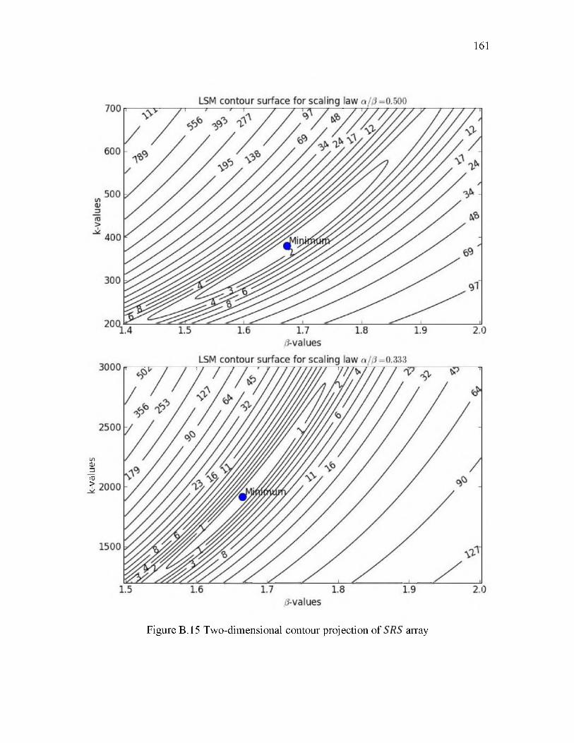
k-valu

es

161

Figure B.15 Two-dimensional contour projection of array

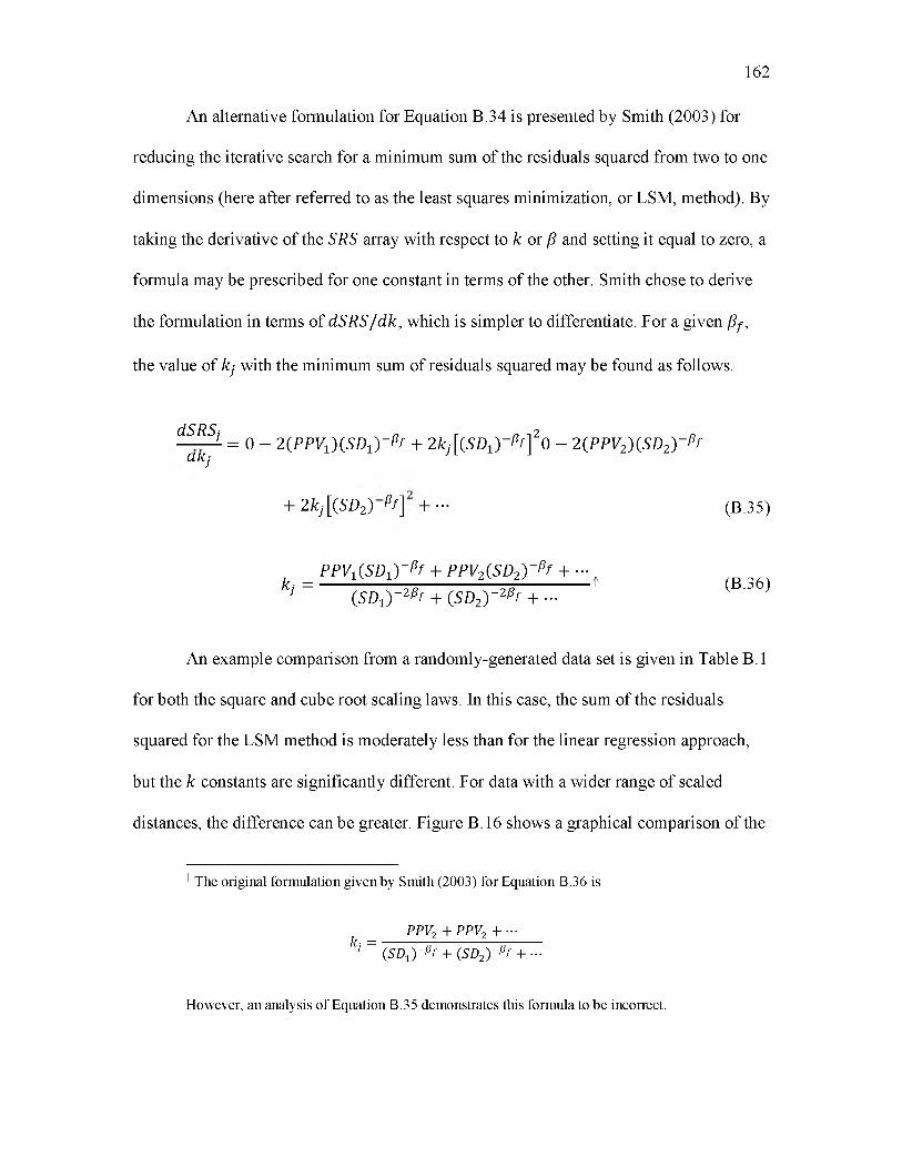
An alternative formulation for Equation B.34 is presented by Smith (2003) for

reducing the iterative search for a minimum sum of the residuals squared from two to one

dimensions (here after referred to as the least squares minimization, or LSM, method). By

taking the derivative of the SRS array with respect to k or / and setting it equal to zero, a

formula may be prescribed for one constant in terms of the other. Smith chose to derive

the formulation in terms of -S R S / dk, which is simpler to differentiate. For a given / y,

the value of k- with the minimum sum of residuals squared may be found as follows.

162

dS RS- — j- = 0 - 2(PPV1 )(SD1) -pf + 2 kj [(SD1 ) -pf ] 0 - 2 (PPVv)(SDv) - pf

CLKj

+ 2 k-[(SDv) Pf] + • • • (B.35)

, P P V-(SD , ) - Pf + P P Vv(SDv ) - Pf + • • • +k y = --------------- ---------------------------------- * (B.36)- (SD x) - v P f + (SDv ) - v P f + • • •

An example comparison from a randomly-generated data set is given in Table B. 1

for both the square and cube root scaling laws. In this case, the sum of the residuals

squared for the LSM method is moderately less than for the linear regression approach,

but the k constants are significantly different. For data with a wider range of scaled

distances, the difference can be greater. Figure B.16 shows a graphical comparison of the

t The original formulation given by Smith (2003) for Equation B.36 is

PPV2 + PPV2 + •••kt = ■

- (S D -J- P f + (S D v) - P f + • • •

However, an analysis o f Equation B.35 demonstrates this formula to be incorrect.

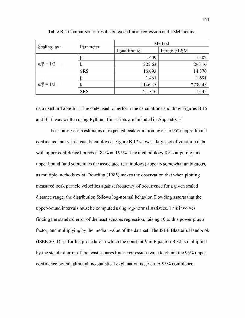
163

Table B. 1 Comparison of results between linear regression and LSM method

Scaling law ParameterMethod

Logarithmic Iterative LSM

=/pa/

P 1.409 1.502k 225.63 295.16SRS 16.693 14.870

/3=/pa/

P 1.461 1.691k 1146.35 2739.45SRS 21.346 15.45

data used in Table B.1. The code used to perform the calculations and draw Figures B.15

and B.16 was written using Python. The scripts are included in Appendix H.

For conservative estimates of expected peak vibration levels, a 95% upper-bound

confidence interval is usually employed. Figure B.17 shows a large set of vibration data

with upper confidence bounds at 84% and 95%. The methodology for computing this

upper bound (and sometimes the associated terminology) appears somewhat ambiguous,

as multiple methods exist. Dowding (1985) makes the observation that when plotting

measured peak particle velocities against frequency o f occurrence for a given scaled

distance range, the distribution follows log-normal behavior. Dowding asserts that the

upper-bound intervals must be computed using log-normal statistics. This involves

finding the standard error of the least squares regression, raising 10 to this power plus a

factor, and multiplying by the median value of the data set. The ISEE Blaster’s Handbook

(ISEE 2011) set forth a procedure in which the constant k in Equation B.32 is multiplied

by the standard error of the least squares linear regression twice to obtain the 95% upper

confidence bound, although no statistical explanation is given. A 95% confidence

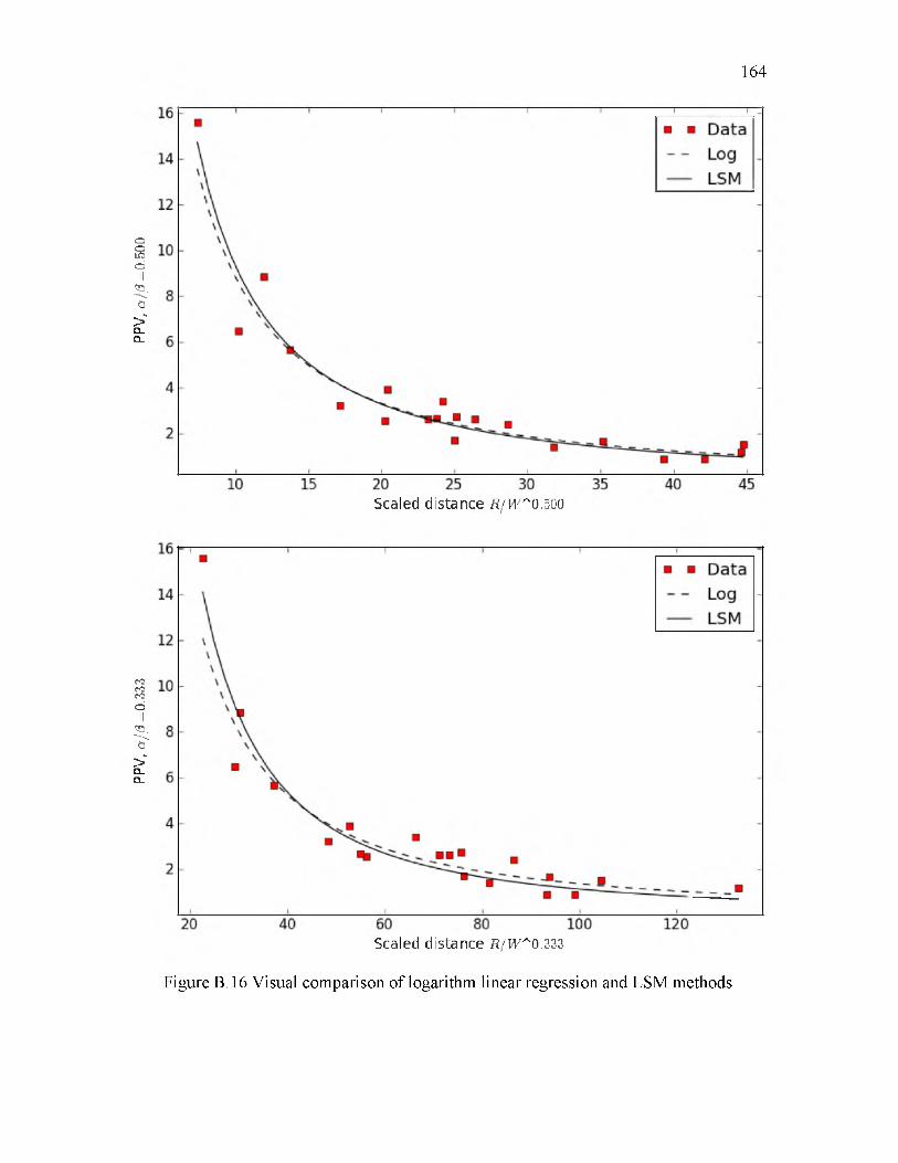
PPV,

a//?

=0.33

3 PP

V, «//

? =0

.500

164

Scaled distance f l / r 0.500

Scaled distance R /W *0.333

Figure B.16 Visual comparison of logarithm linear regression and LSM methods

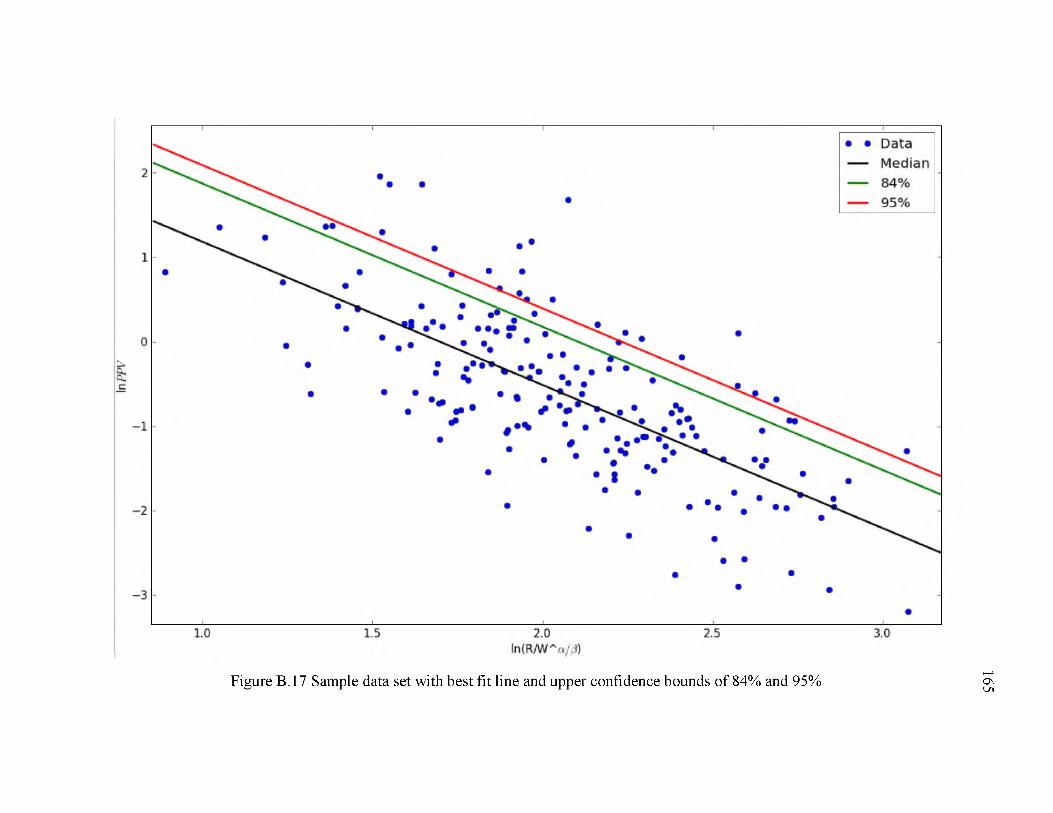
Figure B.17 Sample data set with best fit line and upper confidence bounds of 84% and 95%

165

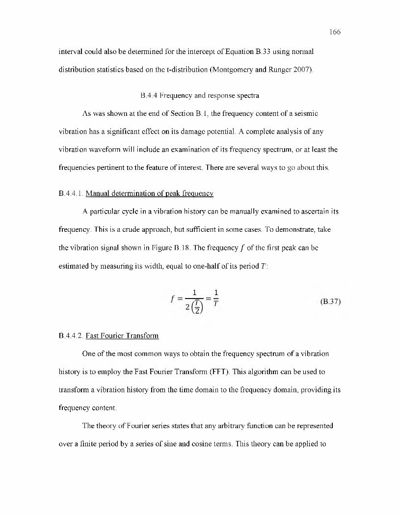
interval could also be determined for the intercept of Equation B.33 using normal

distribution statistics based on the t-distribution (Montgomery and Runger 2007).

B.4.4 Frequency and response spectra

As was shown at the end of Section B.1, the frequency content of a seismic

vibration has a significant effect on its damage potential. A complete analysis of any

vibration waveform will include an examination of its frequency spectrum, or at least the

frequencies pertinent to the feature of interest. There are several ways to go about this.

B.4.4.1. Manual determination of peak frequency

A particular cycle in a vibration history can be manually examined to ascertain its

frequency. This is a crude approach, but sufficient in some cases. To demonstrate, take

the vibration signal shown in Figure B.18. The frequency f of the first peak can be

estimated by measuring its width, equal to one-half of its period T :

166

1 1

B.4.4.2. Fast Fourier Transform

One of the most common ways to obtain the frequency spectrum of a vibration

history is to employ the Fast Fourier Transform (FFT). This algorithm can be used to

transform a vibration history from the time domain to the frequency domain, providing its

frequency content.

The theory of Fourier series states that any arbitrary function can be represented

over a finite period by a series of sine and cosine terms. This theory can be applied to

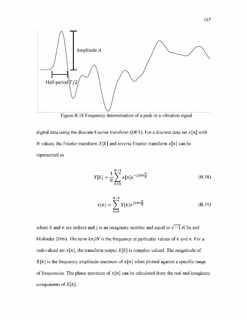
167

digital data using the discrete Fourier transform (DFT). For a discrete data set x [n] with

N values, the Fourier transform X [k] and inverse Fourier transform x [n] can be

represented as

w-i

X [k ] = ^ Z x M e_ }2nk* (B38)71 = 0

w - i

x [n] = ^ X [k] e }2nkTi (B.39)k=0

where k and n are indices and j is an imaginary number and equal to V—1 (Cha and

Molinder 2006). The term kn / N is the frequency at particular values of k and n. For a

real-valued set x [n] , the transform output X [k] is complex valued. The magnitude of

X [k ] is the frequency amplitude spectrum of x [n] when plotted against a specific range

of frequencies. The phase spectrum of can be calculated from the real and imaginary

components of .

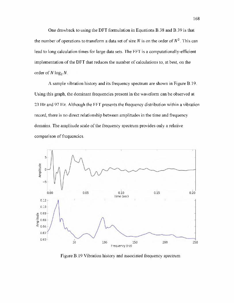
One drawback to using the DFT formulation in Equations B.38 and B.39 is that

the number of operations to transform a data set of size N is on the order of N 2. This can

lead to long calculation times for large data sets. The FFT is a computationally-efficient

implementation of the DFT that reduces the number of calculations to, at best, on the

order of .

A sample vibration history and its frequency spectrum are shown in Figure B.19.

Using this graph, the dominant frequencies present in the waveform can be observed at

23 Hz and 97 Hz. Although the FFT presents the frequency distribution within a vibration

record, there is no direct relationship between amplitudes in the time and frequency

domains. The amplitude scale of the frequency spectrum provides only a relative

comparison of frequencies.

168

Time (sec)0.12

0.10

aj 0.08T3f 0.06 E< 0.04

0.02

0.00 fc____________ i______________ i______________ i______________ i_____________ d50 100 150 200 250

Frequency (Hz)

Figure B.19 Vibration history and associated frequency spectrum

A power spectrum may also be computed by taking the square of the frequency

spectrum, or P [k ] = \X [k] |2. Since the energy of a wave is proportional to the square of

its amplitude, the power spectrum can be used to compare the energy content of a wave

as partitioned by frequency.

B.4.4.3. Response spectra

Response spectra can be used to evaluate the frequency content of a vibration

history. A response spectra analysis is similar to Fourier spectrum analysis in that both

show the distribution of frequencies. However, response spectra have the added

advantage of being able to directly correlate ground motion amplitude with frequency.

Response spectra analysis is more widely used in evaluating structural response, but can

be applied to ground motion as well.

Response spectra analysis is based on a single-degree-of-freedom (SDF)

mathematical system (Dowding 1985). The governing differential equation is that for a

2nd order mechanical oscillating system, as shown below.

mx + c8 + k 8 = 0 (B.40)

where

x is the acceleration of mass m,

c is the damping coefficient,

k is the spring constant,

8 = x — u is the relative displacement of mass m with respect to the ground,

8 is the velocity of mass m with respect to the ground, and

u is the displacement of the ground.

169

Equation B.40 can be recast as

S + 2 /p S + p 2S = u (B.41)

where

S is the acceleration of mass m with respect to the ground,

170

p = ^ k / m is the angular natural frequency of the undamped spring-mass system,

/ = is the fraction of critical damping 2Vkm, and

u is the ground acceleration.

To determine the response spectrum of a particular velocity vibration history

u ( t) , the following integral can be used, provided that S and S are zero at the start time

t 0 (Dowding 1985).

S (t)

L

= - / U W e _ M M )

/cos[pd( t - r ) ] - sin[pd( t - r ) ]

V 1 - / 2d r (B.42)

where

t is the time interval,

r is the dummy variable within the integral representing time, and

pd = p V l - / 2 is the angular natural frequency of the damped spring-mass system.

Equation B.42 predicts the ground motion in terms of relative displacement, not

absolute velocity (Dowding 1985). To estimate the particle velocity S (t), an

approximation can be made in multiplying the maximum value of S (t) by the angular

natural frequency p = 2 ^ / , where / is the natural frequency in Hz.

(B.43)

171

This term S( t ) is called the pseudovelocity or pseudospectral response velocity. It is an

approximation based on simple sinusoidal motion, much like that discussed in Section

B.1. Figure B.20 shows sample response spectra for two blast-generated vibration

histories.

PSEU

OO

VEL

OC

ITY,

in/«

e

172

STRUCTURE NATURAL FREQUENCY, Hx

Figure B.20 Response spectra from two different blast vibration records (Source: Siskind et al. 1980. Courtesy of the U.S. Bureau of Mines).

APPENDIX C

MEASURING BLAST INDUCED DAMAGE

A wide variety of methods for measuring blast-induced damage in the field have

been tried with varying degrees of accuracy and success. Measurement techniques can be

divided into two categories: direct measurements and indirect measurements. For the

purposes of this thesis, the distinction is defined as follows:

• Direct measurements involve direct observations of damage or of the blast

event. Examples include vibration records, fracture observations, bench

dilation, and so forth.

• Indirect measurements involve analyzing changes in rock properties

resulting from the blast damage mechanism. These include methods to

measure alterations in wave transmissions, strength, permeability, and

geophysical properties.

When deciding on the types of measurements needed for conducting a blast

damage study, a number of factors must be considered. Some methods can be easily

employed during normal mining activities. Others are more labor intensive and/or

expensive and are currently useful only for research purposes. The reliability of each

method is important knowledge, both in terms of equipment and the nature of the

measurements themselves. Equipment must be tested and, if appropriate, calibrated

beforehand. Some methods may be highly sensitive to laboratory or field conditions such

as temperature, weather, and durability, which must be taken into account. Because of the

violent nature of blasting, instruments employed in near-field measurements can

potentially be damaged or destroyed or otherwise unrecoverable.

Each method is tailored towards measuring a particular variable. No one

technique can give a comprehensive assessment of blast damage. In any experimental

174

study of blast damage, an appropriate selection of variables or indicators to delineate

between intact and damaged rock will need to be made.

C.1 Direct measurements

C.1.1 Vibration

One of the most common means of measuring blast damage, both near-field and

far-field, is by vibration measurements. Studies in the mid- to late-1900s primarily

focused on the effects of vibrations to structures. A more recent emphasis has been

placed on near-field blast-induced damage in the scientific community, and with it

vibration as a damage criterion continues to be widely-incorporated. While vibrations do

not directly measure damage in the ground, they do provide a record of the ground

motion. Through knowledge of the mechanical properties of the ground and the use of

appropriate constitutive laws, these vibrations can be mathematically related to solid

material behavior and thus failure models.

Two of the most common variables used to assess the possibility of failure are

strain and strain rate. All solids eventually yield and/or fail when undergoing sufficient

deformation. Rocks, being brittle, tend to fail at smaller strains than other solids such as

metals. The magnitude of strain, and consequently stress, that a material can sustain is in

part influenced by the strain rate. Studies on the behavior of solids under different

loading rates show that the strengths of dynamically-loaded test specimens can be several

times higher than for quasistatically loaded ones (Sun 2013). All three of the kinematic

descriptors of vibration discussed in Section B.1 of Appendix B can be related to strain

and/or strain rate.

175

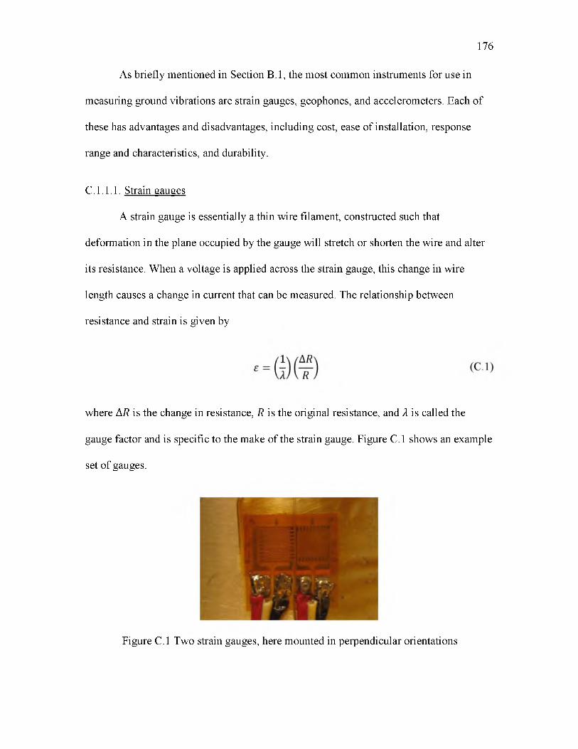
As briefly mentioned in Section B.1, the most common instruments for use in

measuring ground vibrations are strain gauges, geophones, and accelerometers. Each of

these has advantages and disadvantages, including cost, ease of installation, response

range and characteristics, and durability.

C.1.1.1. Strain gauges

A strain gauge is essentially a thin wire filament, constructed such that

deformation in the plane occupied by the gauge will stretch or shorten the wire and alter

its resistance. When a voltage is applied across the strain gauge, this change in wire

length causes a change in current that can be measured. The relationship between

resistance and strain is given by

176

where AR is the change in resistance, R is the original resistance, and X is called the

gauge factor and is specific to the make of the strain gauge. Figure C. 1 shows an example

set of gauges.

Figure C.1 Two strain gauges, here mounted in perpendicular orientations

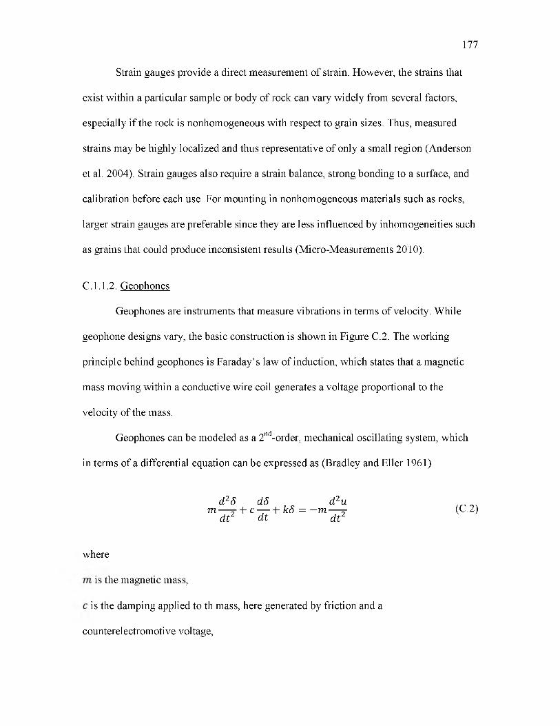
Strain gauges provide a direct measurement of strain. However, the strains that

exist within a particular sample or body of rock can vary widely from several factors,

especially if the rock is nonhomogeneous with respect to grain sizes. Thus, measured

strains may be highly localized and thus representative of only a small region (Anderson

et al. 2004). Strain gauges also require a strain balance, strong bonding to a surface, and

calibration before each use. For mounting in nonhomogeneous materials such as rocks,

larger strain gauges are preferable since they are less influenced by inhomogeneities such

as grains that could produce inconsistent results (Micro-Measurements 2010).

C.1.1.2. Geophones

Geophones are instruments that measure vibrations in terms of velocity. While

geophone designs vary, the basic construction is shown in Figure C.2. The working

principle behind geophones is Faraday’s law of induction, which states that a magnetic

mass moving within a conductive wire coil generates a voltage proportional to the

velocity of the mass.

Geophones can be modeled as a 2nd-order, mechanical oscillating system, which

in terms of a differential equation can be expressed as (Bradley and Eller 1961)

d 28 d8 d 2um — T + c — + k S = — m — (C. 2)

d t 2 d t d t 2

where

is the magnetic mass,

is the damping applied to th mass, here generated by friction and a

counterelectromotive voltage,

177

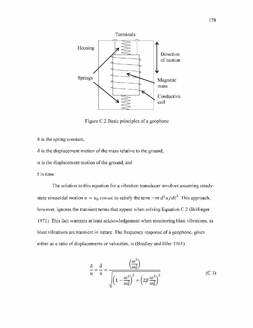
178

Terminals

Housing

Springs

X Conductive coil

Magneticmass

Direction of motion

Figure C.2 Basic principles of a geophone

k is the spring constant,

S is the displacement motion of the mass relative to the ground,

u is the displacement motion of the ground, and

t is time.

The solution to this equation for a vibration transducer involves assuming steady-

state sinusoidal motion u = u 0 cos w t to satisfy the term - m d 2u / d t . This approach,

however, ignores the transient terms that appear when solving Equation C.2 (Bollinger

1971). This fact warrants at least acknowledgement when monitoring blast vibrations, as

blast vibrations are transient in nature. The frequency response of a geophone, given

either as a ratio of displacements or velocities, is (Bradley and Eller 1961)

u uS S

(C.3)

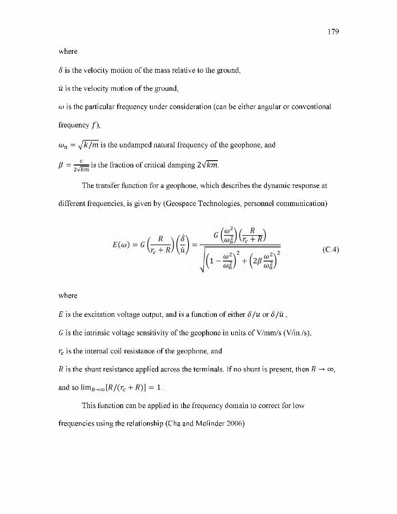
179

where

S is the velocity motion of the mass relative to the ground,

u is the velocity motion of the ground,

o is the particular frequency under consideration (can be either angular or conventional

frequency ),

The transfer function for a geophone, which describes the dynamic response at

different frequencies, is given by (Geospace Technologies, personnel communication)

G is the intrinsic voltage sensitivity of the geophone in units of V/mm/s (V/in./s),

rc is the internal coil resistance of the geophone, and

R is the shunt resistance applied across the terminals. If no shunt is present, then R — oo,

and so .

This function can be applied in the frequency domain to correct for low

frequencies using the relationship (Cha and Molinder 2006)

o n = y k /rn is the undamped natural frequency of the geophone, and

/ = is the fraction of critical damping 2 Vk m .

where

E is the excitation voltage output, and is a function of either S /u or S /u ,

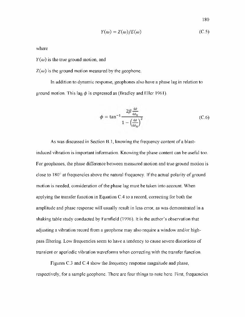
180

Y( m ) = Z ( m ) / E ( m ) (C.5)

where

Y( m ) is the true ground motion, and

Z ( m ) is the ground motion measured by the geophone.

In addition to dynamic response, geophones also have a phase lag in relation to

ground motion. This lag 0 is expressed as (Bradley and Eller 1961).

As was discussed in Section B.1, knowing the frequency content of a blast-

induced vibration is important information. Knowing the phase content can be useful too.

For geophones, the phase difference between measured motion and true ground motion is

close to 180° at frequencies above the natural frequency. If the actual polarity of ground

motion is needed, consideration of the phase lag must be taken into account. When

applying the transfer function in Equation C.4 to a record, correcting for both the

amplitude and phase response will usually result in less error, as was demonstrated in a

shaking table study conducted by Farnfield (1996). It is the author’s observation that

adjusting a vibration record from a geophone may also require a window and/or high-

pass filtering. Low frequencies seem to have a tendency to cause severe distortions of

transient or aperiodic vibration waveforms when correcting with the transfer function.

Figures C.3 and C.4 show the frequency response magnitude and phase,

respectively, for a sample geophone. There are four things to note here. First, frequencies

(C.6)

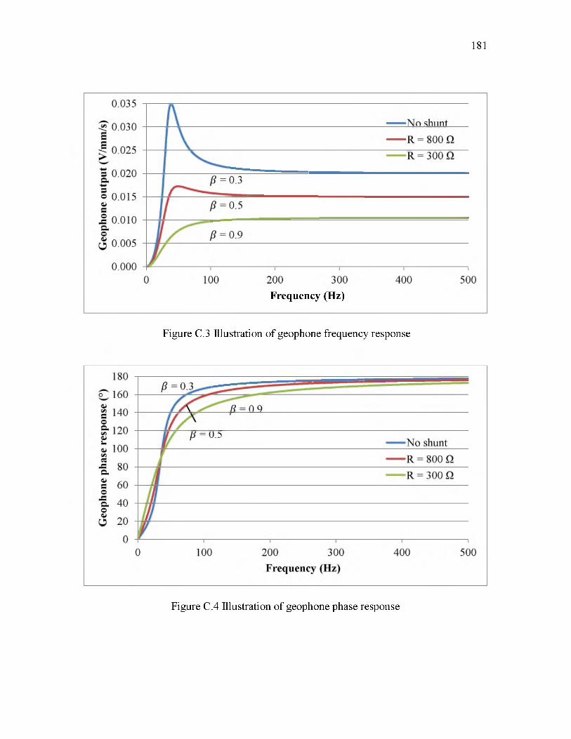
181

Frequency (Hz)

Figure C.3 Illustration of geophone frequency response

Figure C.4 Illustration of geophone phase response

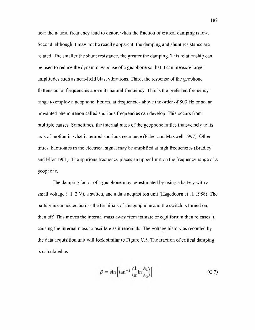
182

near the natural frequency tend to distort when the fraction of critical damping is low.

Second, although it may not be readily apparent, the damping and shunt resistance are

related. The smaller the shunt resistance, the greater the damping. This relationship can

be used to reduce the dynamic response of a geophone so that it can measure larger

amplitudes such as near-field blast vibrations. Third, the response of the geophone

flattens out at frequencies above its natural frequency. This is the preferred frequency

range to employ a geophone. Fourth, at frequencies above the order of 800 Hz or so, an

unwanted phenomenon called spurious frequencies can develop. This occurs from

multiple causes. Sometimes, the internal mass of the geophone rattles transversely to its

axis of motion in what is termed spurious resonance (Faber and Maxwell 1997). Other

times, harmonics in the electrical signal may be amplified at high frequencies (Bradley

and Eller 1961). The spurious frequency places an upper limit on the frequency range of a

geophone.

The damping factor of a geophone may be estimated by using a battery with a

small voltage (~1-2 V), a switch, and a data acquisition unit (Hagedoorn et al. 1988). The

battery is connected across the terminals of the geophone and the switch is turned on,

then off. This moves the internal mass away from its state of equilibrium then releases it,

causing the internal mass to oscillate as it rebounds. The voltage history as recorded by

the data acquisition unit will look similar to Figure C.5. The fraction of critical damping

is calculated as

(C.7)

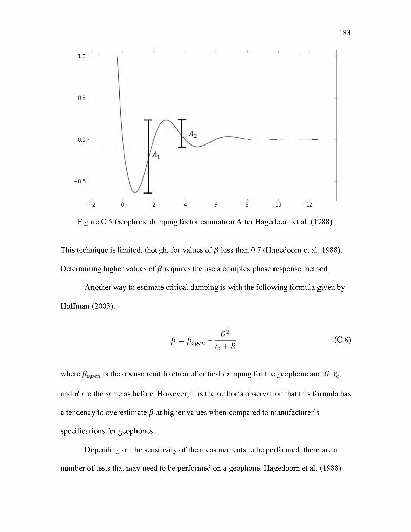
1.0 -

0.5 -

0.0 -

-0 .5 -

-2 0 2 4 6 8 10 12

Figure C.5 Geophone damping factor estimation After Hagedoorn et al. (1988).

This technique is limited, though, for values of / less than 0.7 (Hagedoorn et al. 1988).

Determining higher values of requires the use a complex phase response method.

Another way to estimate critical damping is with the following formula given by

Hoffman (2003):

P = Popen + r ^ (C 8)

where is the open-circuit fraction of critical damping for the geophone and , ,

and R are the same as before. However, it is the author’s observation that this formula has

a tendency to overestimate / at higher values when compared to manufacturer’s

specifications for geophones.

Depending on the sensitivity of the measurements to be performed, there are a

number of tests that may need to be performed on a geophone. Hagedoorn et al. (1988)

183

provided the following comprehensive list:

• Conformity to manufacturer’s specifications:

- Resistance,

- Polarity,

- Frequency,

- Damping,

- Sensitivity, and

- Distortion.

• Upper frequency limit as dictated by spurious responses;

• Infiltration of unwanted noise through leakage;

• Stability in maintaining tolerances, even after events such as a shock;

• Sticking coil;

• Dirt, meaning that a something such as small fiber is touching the coil and

thus affecting the geophone’s threshold;

• Sensitivity to temperature variations; and

• Durability with repeated use and adverse field conditions.

Field application of geophones requires several considerations in addition to

calibrating and testing the geophone. Most important among these is the quality of

coupling between the instrument and the ground. Three practices often employed in the

field are burying the instrument in the ground, driving a spike into the ground with the

instrument mounted on the spike, and simply setting the instrument on the ground

(Wheeler 2004). Poor or inadequate coupling will increase error present in vibration

readings, as has been demonstrated through studies such as Segarra et al. (2013) and

184

Wheeler (2004). For near-field blast vibrations, which have large amplitudes, a solid

means of anchoring is required. Options include bolting into a rock outcrop on the

surface, securing downhole using a “foot” that can wedge itself between the borehole

walls, or positioning downhole and the pouring in a grout mixture. In addition to

coupling, the dynamic range of the geophone and the intrinsic noise levels must also be

considered (Badger et al. 1990). Vibrations that exceed the range capability of the

geophone or are below the noise threshold will result in poor measurements.

The response of many geophones is also sensitive to the orientation of the

transducer. Some geophones are unidirection and must be vertical, some can operate at

angles up to 90° from vertical, and some are omnidirectional and can be positioned at any

angle.

C.1.1.3. Accelerometers

Accelerometers measure vibration in terms of acceleration. Their basic

construction consists of a mass mounted on a piezoelectric element, usually made of

quartz or certain kinds of ceramics (PCB Piezotronics 2013 a). Vibrations experienced by

the accelerometer cause the mass to apply a load to the piezoelectric element, which

responds by producing a charge directly proportional to the acceleration. As shown in

Figure C.6, there are three basic configurations in which the piezoelectric element can

deform: compression, shear, and flexure.

Accelerometers cannot be connected to a normal data acquisition system without

first routing the signal through a signal conditioner. The type of signal conditioner that

can be used depends on the electronics included in the accelerometer. There are two main

designs that dictate how the accelerometer operates: charge mode or integrated circuit

185

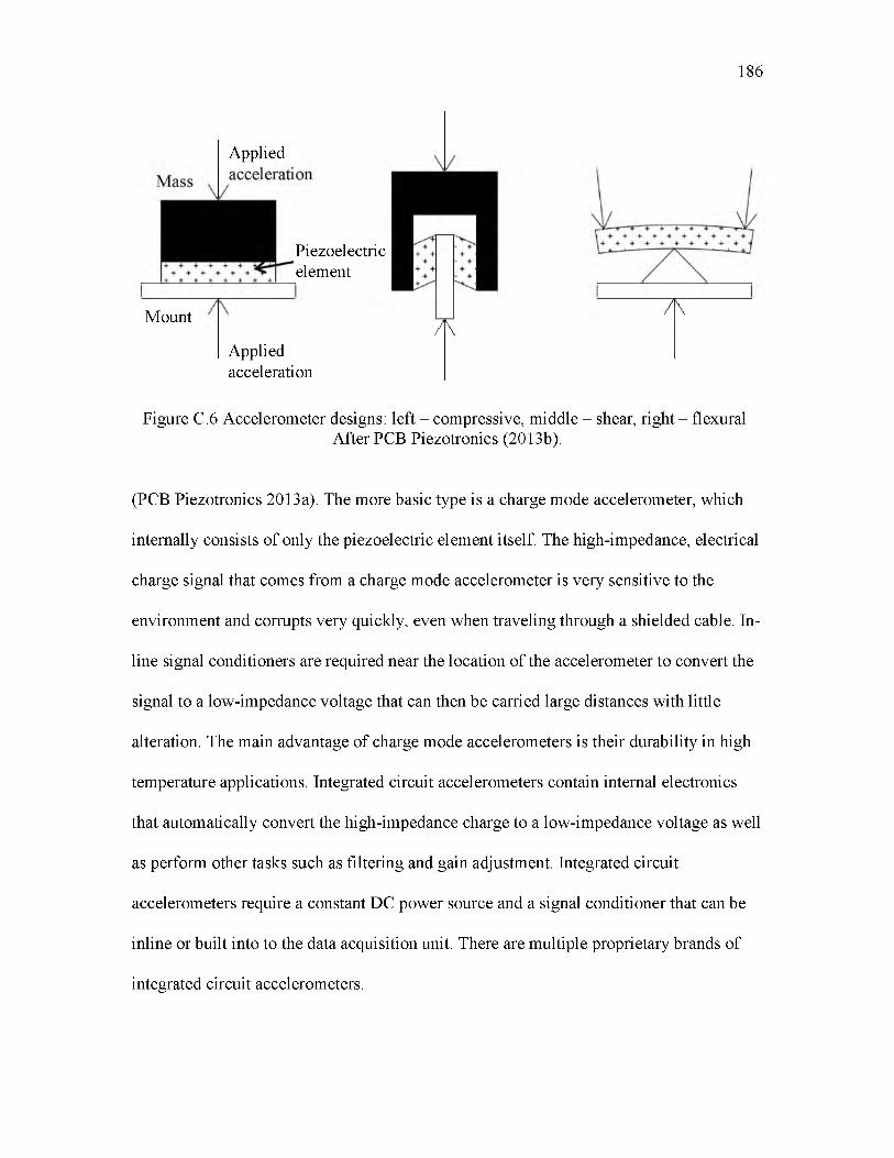
186

Applied

Piezoelectricelement

Mount A7 [\

Appliedacceleration

Figure C.6 Accelerometer designs: left - compressive, middle - shear, right - flexuralAfter PCB Piezotronics (2013b).

(PCB Piezotronics 2013a). The more basic type is a charge mode accelerometer, which

internally consists of only the piezoelectric element itself. The high-impedance, electrical

charge signal that comes from a charge mode accelerometer is very sensitive to the

environment and corrupts very quickly, even when traveling through a shielded cable. In­

line signal conditioners are required near the location of the accelerometer to convert the

signal to a low-impedance voltage that can then be carried large distances with little

alteration. The main advantage of charge mode accelerometers is their durability in high

temperature applications. Integrated circuit accelerometers contain internal electronics

that automatically convert the high-impedance charge to a low-impedance voltage as well

as perform other tasks such as filtering and gain adjustment. Integrated circuit

accelerometers require a constant DC power source and a signal conditioner that can be

inline or built into to the data acquisition unit. There are multiple proprietary brands of

integrated circuit accelerometers.

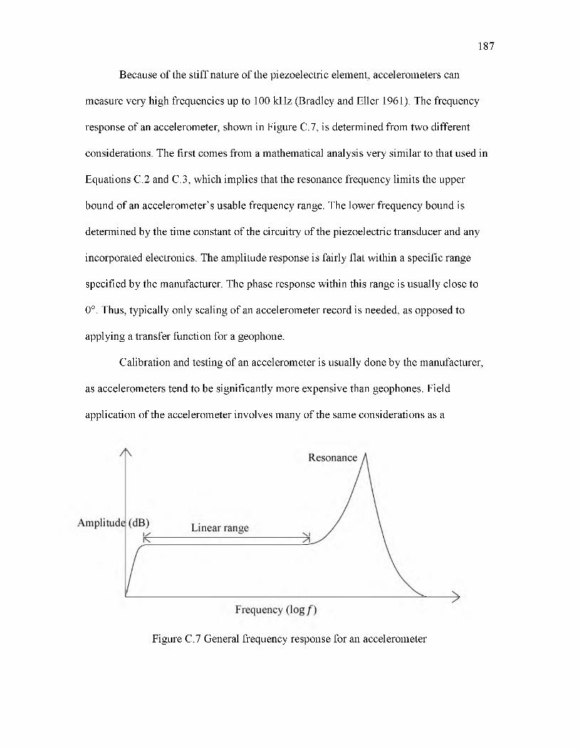
Because of the stiff nature of the piezoelectric element, accelerometers can

measure very high frequencies up to 100 kHz (Bradley and Eller 1961). The frequency

response of an accelerometer, shown in Figure C.7, is determined from two different

considerations. The first comes from a mathematical analysis very similar to that used in

Equations C.2 and C.3, which implies that the resonance frequency limits the upper

bound of an accelerometer’s usable frequency range. The lower frequency bound is

determined by the time constant of the circuitry of the piezoelectric transducer and any

incorporated electronics. The amplitude response is fairly flat within a specific range

specified by the manufacturer. The phase response within this range is usually close to

0°. Thus, typically only scaling of an accelerometer record is needed, as opposed to

applying a transfer function for a geophone.

Calibration and testing of an accelerometer is usually done by the manufacturer,

as accelerometers tend to be significantly more expensive than geophones. Field

application of the accelerometer involves many of the same considerations as a

187

Figure C.7 General frequency response for an accelerometer

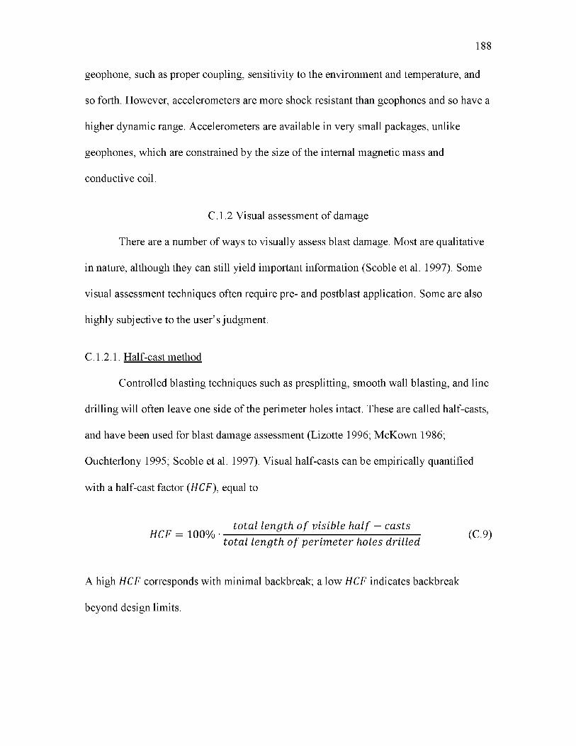
geophone, such as proper coupling, sensitivity to the environment and temperature, and

so forth. However, accelerometers are more shock resistant than geophones and so have a

higher dynamic range. Accelerometers are available in very small packages, unlike

geophones, which are constrained by the size of the internal magnetic mass and

conductive coil.

C.1.2 Visual assessment of damage

There are a number of ways to visually assess blast damage. Most are qualitative

in nature, although they can still yield important information (Scoble et al. 1997). Some

visual assessment techniques often require pre- and postblast application. Some are also

highly subjective to the user’s judgment.

C.1.2.1. Half-cast method

Controlled blasting techniques such as presplitting, smooth wall blasting, and line

drilling will often leave one side of the perimeter holes intact. These are called half-casts,

and have been used for blast damage assessment (Lizotte 1996; McKown 1986;

Ouchterlony 1995; Scoble et al. 1997). Visual half-casts can be empirically quantified

with a half-cast factor (HCF), equal to

188

to ta l lenq th o f v isib le h a l f — cas tsHCF = 1 0 0 % ------- - ------ ------------ :----------t—:---- (C9)

to ta l lenq th o f p e r im e te r holes dr i l led

A high HCF corresponds with minimal backbreak; a low HCF indicates backbreak

beyond design limits.

C.1.2.2. Fracture mapping

Fracture mapping is used to assess the stability characteristics of a slope or tunnel

wall and identify potential weaknesses. Fracture mapping can be used to visually evaluate

the effects of blast damage and draw comparisons between damaged and undamaged rock

faces and between blast rounds. Methods of fracture mapping include line surveys and

photogrammetry. Drawbacks to fracture mapping include limitations in assessing blast

damage beyond the visible surface and challenges in differentiating fractures from

naturally-occurring discontinuities (Scoble et al. 1997). On the laboratory scale, fracture

patterns can be analyzed by using a wire saw to cut through a rock or concrete sample

that has been blasted (Iverson et al. 2010). Drill core inspection can also be performed.

C.1.2.3. Borehole surveys

Surveys of blast-induced fracturing can be conducted downhole using borehole

cameras (Brent and Smith 1996; McKenzie and Holley 2004; Scoble et al. 1997; Yang et

al. 1993). Both pre- and postblast surveys are needed to evaluate newly-formed cracks.

While borehole surveys allow direct observations of fractures otherwise unobservable,

survey holes located close to a blasthole may collapse, rendering the hole inaccessible

(Smith 2003). Borehole surveying also requires specialized equipment that is employable

in the field and small enough to fit inside a drillhole.

C.1.2.4. Overbreak

Blast damage beyond design limits can be quantified as an overbreak percentage

(Scoble et al. 1997; Singh and Lamond 1993). This can be accomplished by comparing

design limits and postexcavation face profile surveys.

189

C.1.3 Rock mass classification methods

Rock mass classification methods are widely used in rock mechanics. Specialized

classification schemes have been developed specifically for the use of assessing blast

damage (Scoble et al. 1997; Paventi et al. 1996). Such methods, which incorporate visual

inspections with other metrics, can be used to appraise the effects of a blast round.

C.1.4 Scaling time

Scaling time, both with mechanical equipment and manual means, has been

studied as a production-friendly technique for assessing damage along a blasting

perimeter (Scoble et al. 1997; Sutherland 1990). The reasoning behind this method is that

the scaling time is a function of scaling area and blast quality (Scoble et al. 1997). Shorter

scaling times should indicate better wall control.

C.1.5 Bench movement

Bench movement can be used as a sign of joint strength loss and block instability

(McKenzie and Holley 2004). Movement can be measurement with extensometers or by

placing movement markers and surveying displacement with a surveying instrument.

McKenzie and Holley (2004) conducted a study in which movement markers were

grouted in boreholes at varying distances and depths behind a series of blasts. Both

dilation and settling of the bench, along with horizontal movement, were observed.

Overall, movement decreased with distance and depth behind the blast in a somewhat

linear fashion.

190

C.1.6 Pressure measurements

A number of studies have been conducted using pressure diaphragm transducers

secured downhole in boreholes adjacent to a bench blast (Brent and Smith 1996;

Menccaci and Farnfield 2003; Peterson 2001). These sensors can be used to measure gas

pressures as the high pressure gases penetrate their way through the fragmented rock

mass. Although not a direct measurement of damage within the rock itself, knowing the

gas pressures within the zone adjacent to a blast can aid in understanding the combined

effects of the shock wave and gas expansion on crack growth and in analyzing flexural

rupture. Brent and Smith (1999) proposed a relationship between gas pressures and the

increase in the volume of a monitoring hole within a fractured bench that could serve as

an indicator of damage.

C.1.7 Time domain reflectometry

A time domain reflectometer (TDR) is an electronic tool used to detect faults,

shorts, and other changes in a cable or conductive wire (AEMC Instruments 2004). It

operates by sending a voltage pulse from one end of the cable and “listening” for echoes

as part or all of the pulse reflects back when changes in impedance are encountered.

Depending on the nature of the impedance change, the reflected signal will vary in shape

and can be used to diagnose its source. Figure C.8 shows a sample set of events that can

be detected. A TDR can also determine the approximate distance d to each event using

the relationship

191

d = V o ^ (C10)

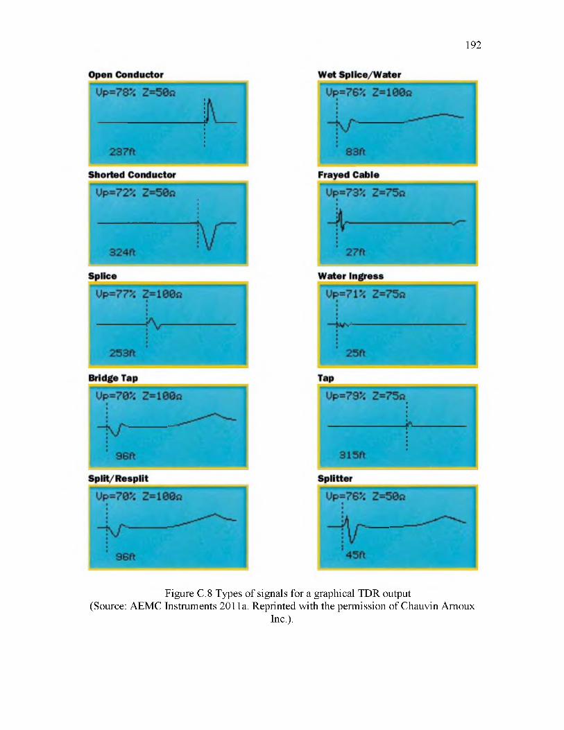
192

Figure C.8 Types of signals for a graphical TDR output (Source: AEMC Instruments 2011a. Reprinted with the permission of Chauvin Arnoux

Inc.).

where

Vp is a calibrated constant called the velocity of propagation and is expressed as a percent

of the speed of light,

c 0 is the speed of light in a vacuum, and

is the two-way travel time for the pulse from the TDR to the event and back.

In theory, the Vp value is a constant for each type of cable or wire and does not

vary with length. For measurements in which multiple types of cables are connected in

series, the following relationship can be derived for an average :

d i + d>2 + (^3 + •••

Vp - averag e = d ^ d _̂ (C. 11)

Vpl VP2 VP2 '

where the Vp constant and distance d for each length of cable is denoted by 1, 2, 3, etc.

Time domain recflectometry has been utilized for assessing blast damage, though

less commonly than most other methods (LeBlanc et al. 1996; Peterson 2001). TDR

readings can give a qualitative indication of movement in the ground, but not exact

displacements. The precision and accuracy of the measurements can be limited by the

resolution of the TDR meter and field conditions such as temperature and the degree of

coupling of the cable in the ground. Signal behavior can also be difficult to interpret at

times. Nonetheless, whereas other methods that rely upon instrumentation positioned near

the blasting are susceptible to damage, the TDR method relies upon such damage for

obtaining measurements and thus can be positioned arbitrarily close without concern.

193

C.2 Indirect measurements

C.2.1 Seismic tomography

Seismic tomography methods can be used to quantify the increase of blast-

induced fractures in a body of rock (Adamson and Scherpenisse 1998; Andrieux et al.

1994; LeBlanc et al. 1996; Singer et al. 2010; Spathis et al. 1987; Trivino and Mohanty

2013; Yang et al. 1993; Zhang and Chang 1999). Seismic tomography measures changes

in the acoustic velocity of rock and the wave attenuation, usually with P-waves. A

decrease in wave velocity often indicates an increase in crack density. Differences in

attenuation rates pre- and postblast also can suggest deterioration of the rock mass from

blasting. Both pre- and postblast surveys are required for this technique to be applicable.

Cross-hole surveys are most commonly employed, in which the body of rock between

two or more nearby holes is analyzed. Downhole-to-surface surveys can also be

performed. Seismic tomography can detect changes from both micro- and

macrofracturing. It is a relatively popular method as it can be used in the field with

minimal setup, provided the appropriate equipment is available. It also produces a fairly

complete picture of the damage zone if the observation holes are adequately located.

C.2.2 Ultrasonic P-wave velocity

Ultrasonic measurements of P-wave velocity in rock samples pre- and postblast

have been used successfully for detecting shock-damaged rock (Hamdi et al. 2003;

Iverson et al. 2010; Kilebrant et al. 2010; Kim and McCarter 1993). Similar to seismic

tomography, the underlying principle is that P-wave velocity decreases as fracture density

increases. However, this method requires that core samples be obtained from the test site,

which requires additional labor and equipment.

194

C.2.3 Permeability

Permeability has been used to assess the zone of damage from blasting (Kelsall et

al. 1984; Pusch and Stanfors 1996). Measurements are made in the field of the in situ

hydraulic conductivity. Care must be taken to control field conditions; otherwise, results

obtained may not reliable. Hydraulic conductivity is also affected by fracture and joint

orientation.

C.2.4 Porosity

Porosity of rock samples pre- and postblast have been measured to indicate blast

damage (Hamdi et al. 2003; Kilebrant et al. 2010). When rocks undergo intense blast-

loading, the resulting fractures increase the rock’s inherent porosity. Porosity

measurements can be made in conjunction with ultrasonic velocity measurements since

both rely on the same phenomenon.

C.2.5 Acoustic emissions

Acoustic emissions (AE) are a phenomenon that occurs during loading of a brittle

rock sample (Seto et al. 1996). Under high stresses, localized failures of the rock as a

microcrack forms or a pore collapses will emit a high-frequency elastic wave called an

AE. If the rock sample is unloaded and then reloaded, AE will not occur until the rock is

loaded past its previous maximum stress state. This is called the Kaiser effect. Given this

behavior, AE can be used to give an accurate assessment of rock damage (Holcomb et al.

1990; Seto et al. 1996). However, this method requires rock sample preparation, a triaxial

loading machine, and piezoelectric transducers that can measure very high frequencies in

195

the hundreds of kHz (Seto et al. 1996). This makes AE useful only for research

investigations.

C.2.6 Ground penetrating radar

Ground penetrating radar can be used to gauge the depth of damage in rock.

Adams et al. (1993) used ground penetrating radar to determine the effects of

preconditioning ahead of a stope face. Ryu et al. (2013) performed a borehole radar

reflection survey to determine the extension of fractures from blasting in a tunneling

project. Ground penetrating radar requires both pre- and postblast surveys to measure

increases in fracture density within the rock.

C.2.7 Electrical resistivity

Electrical resistivity (ER) has been used to gauge the depth of blast-induced rock

damage (Ouchterlony et al. 1993; Scott et al. 1968). The theory is that greater fracture

density will increase the resistivity of the rock. A study conducted by Ouchterlony et al.

(1993) remarked that ER is sensitive enough to detect the presence of a single crack, and

ER results correlated well with borehole fracture inspections. However, as noted by Scott

et al. (1968), electrical resistivity methods are sensitive to the presence of water.

196

APPENDIX D

INTRODUCTION TO PYTHON

Since the reader may not be familiar with Python, a brief introduction is presented

here. Python is a general-purpose, dynamic, high-level programming language that is also

open-source, essentially free for both private and commercial use (Python Software

Foundation 2013). It parses code via an interpreter writing in the C programming

language. In addition to the built-in abilities of Python, there are numerous modules

available to add a plethora of capabilities. Users can also write their own custom

modules. One particular list of Python modules for Windows that the author found

helpful is maintained online by Gohkle (n.d.).

Python 2.7 was used to meet the majority of programming requirements for this

thesis. Python 3.2 was also available at the time, but certain modules desired by the

author had not yet been updated to be compatible with the newer version of Python. For

this thesis, the author heavily utilized the following modules and add-ons:

• Numpy - A numeric processing toolkit with higher-level math functions

and built-in data types that allow for rapid computing, particularly large

arrays and matrices.

• IPython - An interpreter based on the original Python interpreter, but with

additional features and a more detailed output, particularly when

debugging.

• Matplotlib - A plotting toolkit that in some respects emulates

MATLAB®’s plotting environment, but with far more capabilities.

Matplotlib functionality requires the Numpy module.

• SciPy - An advanced scientific computational toolkit with a wide variety

of algorithms and mathematical tools for tasks involving optimization,

198

solvers, signal and image processing, interpolation, linear algebra, etc.

SciPy functionality requires the Numpy module.

• Spyder - An interactive development environment (IDE) that may seem

reminiscent of MATLAB®’s IDE, but with substantially different features.

The simplest way to obtain a complete and fully-functional scientific computing

package is to obtain a compiled distribution called Python(x,y), available online at

http://code.google.com/p/pythonxy/wiki/Welcome (Accessed May 2013). The author,

however, did not use this package, for at the time it was only available in 32-bit, and 64-

bit capability was desired.

Numerous resources are available on the Internet for learning and referencing the

Python language, should the reader wish to understand the flow of the following scripts.

Some details are briefly mentioned here to readily aid the uninitiated reader.

• Comments can be demarcated in three ways:

- With three sets of double quotation marks on each side:

“““Comment 1”””,

- With three sets of single quotation marks on each side:

‘‘‘Comment 2’’’,

- With a number sign at the beginning of each line: # Comment 3.

• Appropriate indentation is enforced in Python, especially within function

definitions and flow control statements such as for loops, while loops, and

if statements.

• Python uses base-0 indexing in arrays, lists, and tuples.

199

APPENDIX E

ROCK MECHANICS TESTING PROGRAM

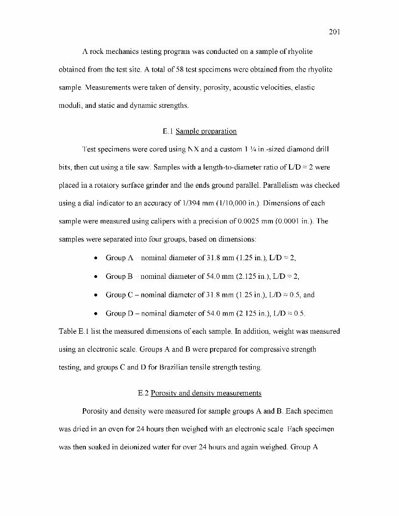
A rock mechanics testing program was conducted on a sample of rhyolite

obtained from the test site. A total of 58 test specimens were obtained from the rhyolite

sample. Measurements were taken of density, porosity, acoustic velocities, elastic

moduli, and static and dynamic strengths.

E.1 Sample preparation

Test specimens were cored using NX and a custom 1 H in.-sized diamond drill

bits, then cut using a tile saw. Samples with a length-to-diameter ratio of L/D ~ 2 were

placed in a rotatory surface grinder and the ends ground parallel. Parallelism was checked

using a dial indicator to an accuracy of 1/394 mm (1/10,000 in.). Dimensions of each

sample were measured using calipers with a precision of 0.0025 mm (0.0001 in.). The

samples were separated into four groups, based on dimensions:

• Group A - nominal diameter of 31.8 mm (1.25 in.), L/D ~ 2,

• Group B - nominal diameter of 54.0 mm (2.125 in.), L/D ~ 2,

• Group C - nominal diameter of 31.8 mm (1.25 in.), L/D ~ 0.5, and

• Group D - nominal diameter of 54.0 mm (2.125 in.), L/D ~ 0.5.

Table E.1 list the measured dimensions of each sample. In addition, weight was measured

using an electronic scale. Groups A and B were prepared for compressive strength

testing, and groups C and D for Brazilian tensile strength testing.

E.2 Porosity and density measurements

Porosity and density were measured for sample groups A and B. Each specimen

was dried in an oven for 24 hours then weighed with an electronic scale. Each specimen

was then soaked in deionized water for over 24 hours and again weighed. Group A

201

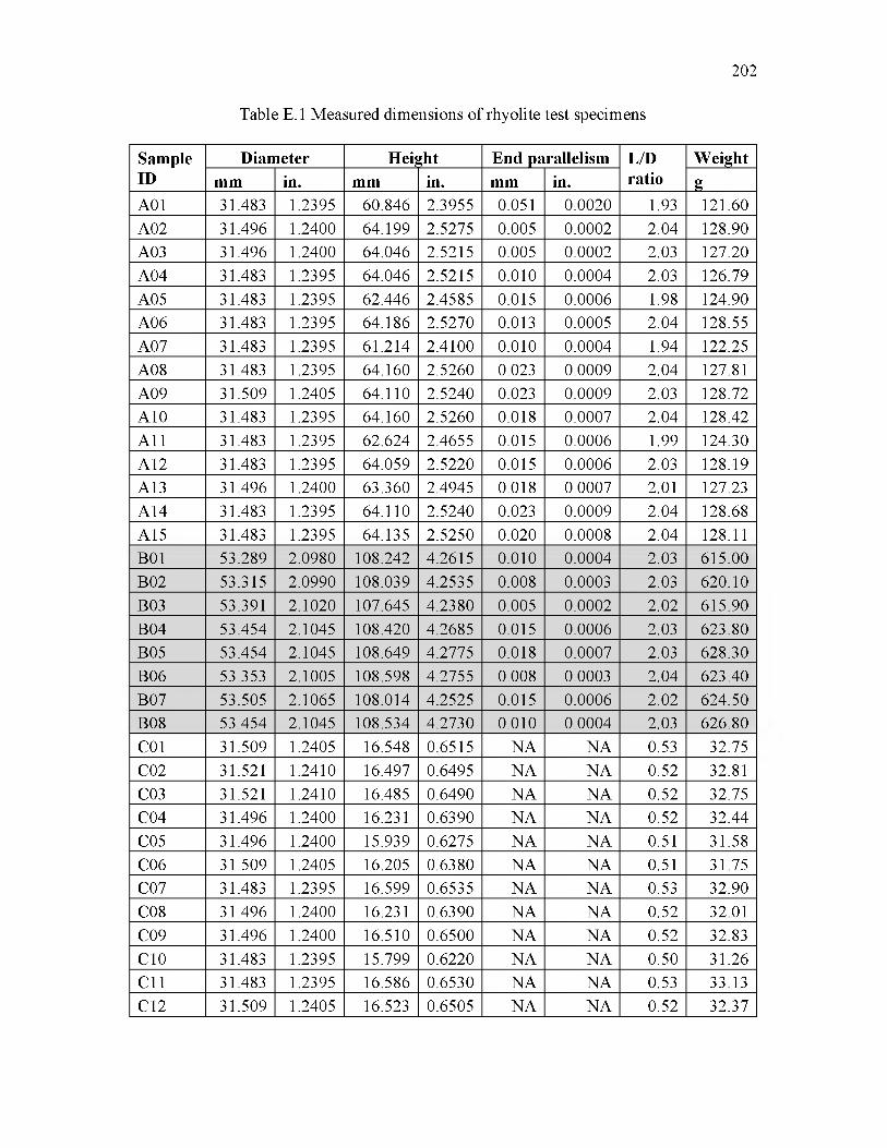
202

Table E.1 Measured dimensions of rhyolite test specimens

SampleID

Diameter Height End parallelism L/Dratio

Weightmm in. mm in. mm in. g

A01 31.483 1.2395 60.846 2.3955 0.051 0.0020 1.93 121.60A02 31.496 1.2400 64.199 2.5275 0.005 0.0002 2.04 128.90A03 31.496 1.2400 64.046 2.5215 0.005 0.0002 2.03 127.20A04 31.483 1.2395 64.046 2.5215 0.010 0.0004 2.03 126.79A05 31.483 1.2395 62.446 2.4585 0.015 0.0006 1.98 124.90A06 31.483 1.2395 64.186 2.5270 0.013 0.0005 2.04 128.55A07 31.483 1.2395 61.214 2.4100 0.010 0.0004 1.94 122.25A08 31.483 1.2395 64.160 2.5260 0.023 0.0009 2.04 127.81A09 31.509 1.2405 64.110 2.5240 0.023 0.0009 2.03 128.72A10 31.483 1.2395 64.160 2.5260 0.018 0.0007 2.04 128.42A11 31.483 1.2395 62.624 2.4655 0.015 0.0006 1.99 124.30A12 31.483 1.2395 64.059 2.5220 0.015 0.0006 2.03 128.19A13 31.496 1.2400 63.360 2.4945 0.018 0.0007 2.01 127.23A14 31.483 1.2395 64.110 2.5240 0.023 0.0009 2.04 128.68A15 31.483 1.2395 64.135 2.5250 0.020 0.0008 2.04 128.11B01 53.289 2.0980 108.242 4.2615 0.010 0.0004 2.03 615.00B02 53.315 2.0990 108.039 4.2535 0.008 0.0003 2.03 620.10B03 53.391 2.1020 107.645 4.2380 0.005 0.0002 2.02 615.90B04 53.454 2.1045 108.420 4.2685 0.015 0.0006 2.03 623.80B05 53.454 2.1045 108.649 4.2775 0.018 0.0007 2.03 628.30B06 53.353 2.1005 108.598 4.2755 0.008 0.0003 2.04 623.40B07 53.505 2.1065 108.014 4.2525 0.015 0.0006 2.02 624.50B08 53.454 2.1045 108.534 4.2730 0.010 0.0004 2.03 626.80C01 31.509 1.2405 16.548 0.6515 NA NA 0.53 32.75C02 31.521 1.2410 16.497 0.6495 NA NA 0.52 32.81C03 31.521 1.2410 16.485 0.6490 NA NA 0.52 32.75C04 31.496 1.2400 16.231 0.6390 NA NA 0.52 32.44C05 31.496 1.2400 15.939 0.6275 NA NA 0.51 31.58C06 31.509 1.2405 16.205 0.6380 NA NA 0.51 31.75C07 31.483 1.2395 16.599 0.6535 NA NA 0.53 32.90C08 31.496 1.2400 16.231 0.6390 NA NA 0.52 32.01C09 31.496 1.2400 16.510 0.6500 NA NA 0.52 32.83C10 31.483 1.2395 15.799 0.6220 NA NA 0.50 31.26C11 31.483 1.2395 16.586 0.6530 NA NA 0.53 33.13C12 31.509 1.2405 16.523 0.6505 NA NA 0.52 32.37

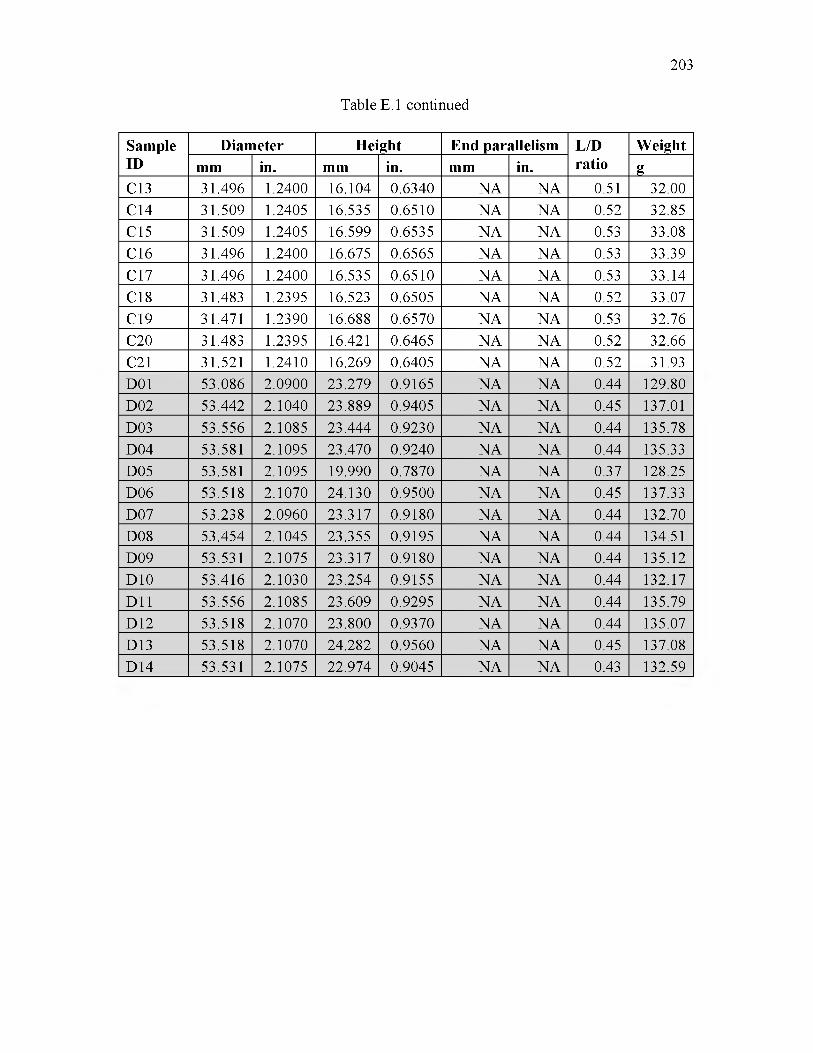
203

Table E.1 continued

SampleID

Diameter Height End parallelism L/Dratio

Weightmm in. mm in. mm in. g

C13 31.496 1.2400 16.104 0.6340 NA NA 0.51 32.00C14 31.509 1.2405 16.535 0.6510 NA NA 0.52 32.85C15 31.509 1.2405 16.599 0.6535 NA NA 0.53 33.08C16 31.496 1.2400 16.675 0.6565 NA NA 0.53 33.39C17 31.496 1.2400 16.535 0.6510 NA NA 0.53 33.14C18 31.483 1.2395 16.523 0.6505 NA NA 0.52 33.07C19 31.471 1.2390 16.688 0.6570 NA NA 0.53 32.76C20 31.483 1.2395 16.421 0.6465 NA NA 0.52 32.66C21 31.521 1.2410 16.269 0.6405 NA NA 0.52 31.93D01 53.086 2.0900 23.279 0.9165 NA NA 0.44 129.80D02 53.442 2.1040 23.889 0.9405 NA NA 0.45 137.01D03 53.556 2.1085 23.444 0.9230 NA NA 0.44 135.78D04 53.581 2.1095 23.470 0.9240 NA NA 0.44 135.33D05 53.581 2.1095 19.990 0.7870 NA NA 0.37 128.25D06 53.518 2.1070 24.130 0.9500 NA NA 0.45 137.33D07 53.238 2.0960 23.317 0.9180 NA NA 0.44 132.70D08 53.454 2.1045 23.355 0.9195 NA NA 0.44 134.51D09 53.531 2.1075 23.317 0.9180 NA NA 0.44 135.12D10 53.416 2.1030 23.254 0.9155 NA NA 0.44 132.17D11 53.556 2.1085 23.609 0.9295 NA NA 0.44 135.79D12 53.518 2.1070 23.800 0.9370 NA NA 0.44 135.07D13 53.518 2.1070 24.282 0.9560 NA NA 0.45 137.08D14 53.531 2.1075 22.974 0.9045 NA NA 0.43 132.59

specimens were weighed to a precision of 0.01 g, and group B specimens to a precision

of 0.1 g. Porosity (n) was calculated using the formula

204

n = — = ------------------ « ------------- (E.1)V7 V7 V7 v 7

where

Vv and V7 are the volumes of void space and total volume of the sample, here in cm ,

W and are the saturated and dry sample weights in grams, and

pw is the density of water, equal to 1.00 g/cm .

The average porosities for groups A and B were 0.0238 and 0.0164, respectively.

It is likely that the B samples did not have sufficient time to soak, as they are larger than

the A samples. Thus, for the purposes of this test, only the results from group A were

used. The saturated, dry, and nominal densities for the rhyolite are 2.58 g/cm , 2.56

3 3g/cm , and 2.57 g/cm , respectively. The results are shown in Tables E.2 and E.3. Note:

samples A01 and A02 were not included in this set of measurements.

E.3 P-wave and S-wave velocities

P-wave and S-wave velocities were measured for samples from group A. An

Olympus Panametrics-NDT Model 5072PR pulser-receiver with dual contact V103-RM

transducers was used to create ultrasonic P-waves, and a Model 5073PR pulser-receiver

with dual normal-incident shear wave V153-RM transducers was used to create

ultrasonic S-waves. Both transducers operated at a frequency of 1 MHz. For each setup,

an Agilent Model 54624A oscilloscope was used to display the ultrasonic wave and

select the arrival times. The average P-wave velocity was 4,606 m/s (15,111 ft/s) and the

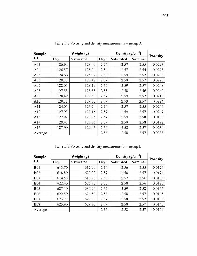
205

Table E.2 Porosity and density measurements - group A

SampleID

Weight (g)3

Density (g/cm )Porosity

Dry Saturated Dry Saturated NominalA03 126.94 128.40 2.54 2.57 2.55 0.0293A04 126.57 128.04 2.54 2.57 2.54 0.0295A05 124.66 125.82 2.56 2.59 2.57 0.0239A06 128.32 129.42 2.57 2.59 2.57 0.0220A07 122.01 123.19 2.56 2.59 2.57 0.0248A08 127.55 128.85 2.55 2.58 2.56 0.0260A09 128.49 129.58 2.57 2.59 2.57 0.0218A10 128.18 129.30 2.57 2.59 2.57 0.0224A11 124.05 125.24 2.54 2.57 2.55 0.0244A12 127.93 129.16 2.57 2.59 2.57 0.0247A13 127.02 127.95 2.57 2.59 2.58 0.0188A14 128.45 129.36 2.57 2.59 2.58 0.0182A15 127.90 129.05 2.56 2.58 2.57 0.0230Average 2.56 2.58 2.57 0.0238

Table E.3 Porosity and density measurements - group B

SampleID

Weight (g)3

Density (g/cm )Porosity

Dry Saturated Dry Saturated NominalB01 613.70 617.90 2.54 2.56 2.55 0.0174B02 618.80 623.00 2.57 2.58 2.57 0.0174B03 614.50 618.90 2.55 2.57 2.56 0.0183B04 622.40 626.90 2.56 2.58 2.56 0.0185B05 627.10 630.90 2.57 2.59 2.58 0.0156B06 622.50 626.50 2.56 2.58 2.57 0.0165B07 623.70 627.00 2.57 2.58 2.57 0.0136B08 625.90 629.30 2.57 2.58 2.57 0.0140Average 2.56 2.58 2.57 0.0164

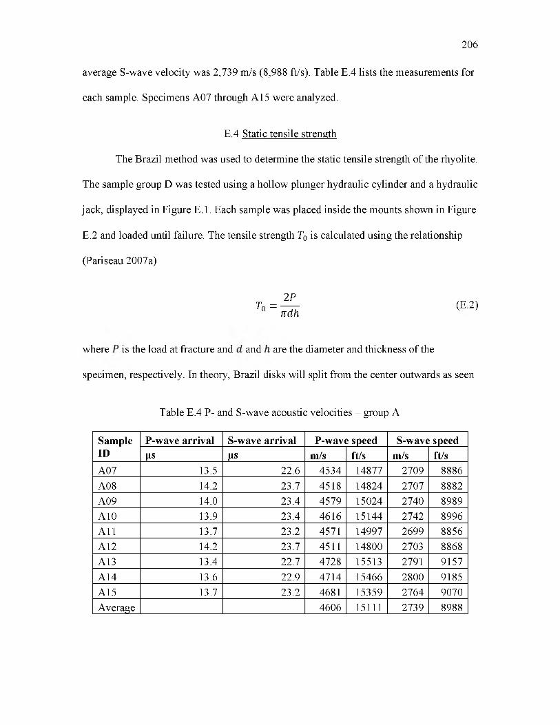
average S-wave velocity was 2,739 m/s (8,988 ft/s). Table E.4 lists the measurements for

each sample. Specimens A07 through A15 were analyzed.

E.4 Static tensile strength

The Brazil method was used to determine the static tensile strength of the rhyolite.

The sample group D was tested using a hollow plunger hydraulic cylinder and a hydraulic

jack, displayed in Figure E.1. Each sample was placed inside the mounts shown in Figure

E.2 and loaded until failure. The tensile strength T0 is calculated using the relationship

(Pariseau 2007a)

206

T0 = ^ (E2)

where is the load at fracture and and are the diameter and thickness of the

specimen, respectively. In theory, Brazil disks will split from the center outwards as seen

Table E.4 P- and S-wave acoustic velocities - group A

SampleID

P-wave arrival S-wave arrival P-wave speed S-wave speed^s ^s m/s ft/s m/s ft/s

A07 13.5 22.6 4534 14877 2709 8886A08 14.2 23.7 4518 14824 2707 8882A09 14.0 23.4 4579 15024 2740 8989A10 13.9 23.4 4616 15144 2742 8996A11 13.7 23.2 4571 14997 2699 8856A12 14.2 23.7 4511 14800 2703 8868A13 13.4 22.7 4728 15513 2791 9157A14 13.6 22.9 4714 15466 2800 9185A15 13.7 23.2 4681 15359 2764 9070Average 4606 15111 2739 8988

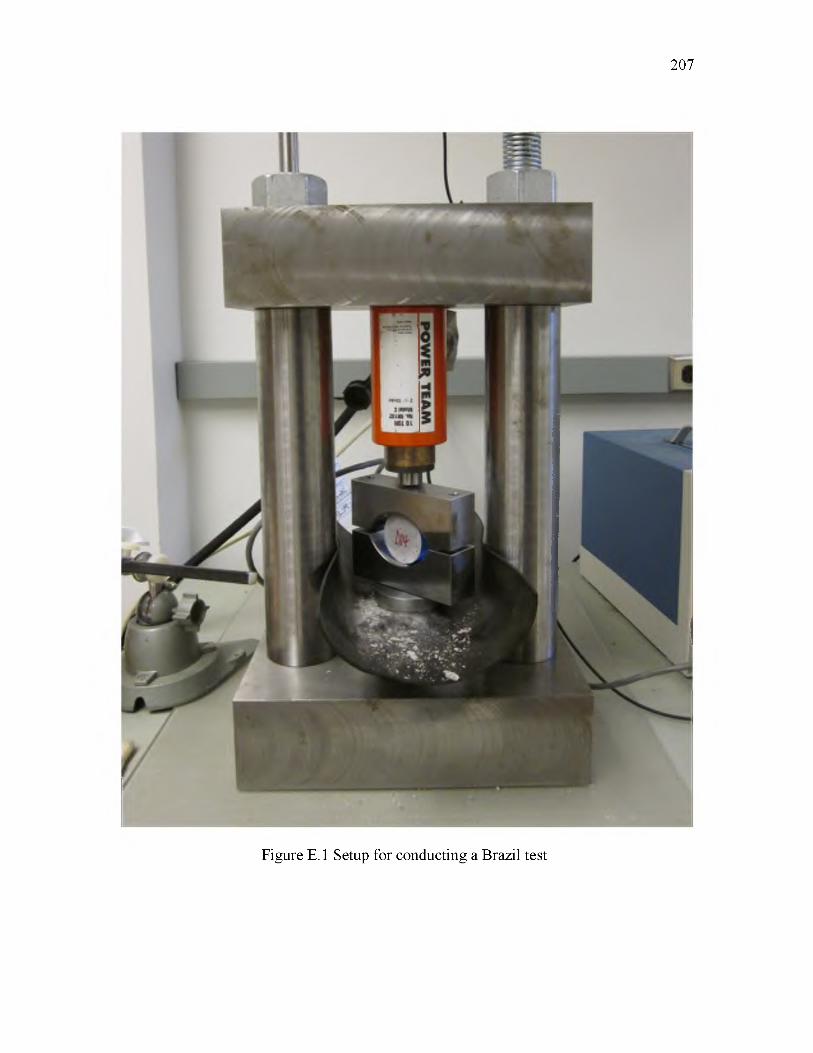
207

Figure E. 1 Setup for conducting a Brazil test

with specimen D04 in Figure E.2. The average tensile strength was 11.30 MPa (1,638

psi). Table E.5 lists the results for the Brazil test.

E.5 Static compressive strength and elastic moduli

A set of tests were conducted using a triaxial compression machine to determine

both unconfined and confined uniaxial compressive strengths, static Young’s modulus,

and Poisson’s ratio. Three A samples and two B samples were loaded, unconfined, to

failure. Two sets of three B samples each were confined in a Hoek cell at two different

confining pressures and loaded until failure. Young’s modulus was determined from the

unconfined compression tests. Strain gauges were mounted on one of the test specimens

to measure axial and transverse strains, which were used to estimate Poisson’s ratio.

208

Figure E.2 Specimen after failure in Brazil test

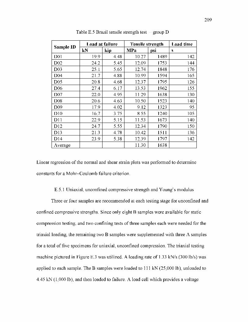
209

Table E.5 Brazil tensile strength test - group D

Sample ID Load at failure Tensile strength Load timekN kip MPa psi s

D01 19.9 4.48 10.27 1489 142D02 24.2 5.45 12.09 1753 144D03 25.1 5.65 12.74 1848 176D04 21.7 4.88 10.99 1594 165D05 20.8 4.68 12.37 1795 126D06 27.4 6.17 13.53 1962 155D07 22.0 4.95 11.29 1638 130D08 20.6 4.63 10.50 1523 140D09 17.9 4.02 9.12 1323 95D10 16.7 3.75 8.55 1240 105D11 22.9 5.15 11.53 1673 140D12 24.7 5.55 12.34 1790 150D13 21.3 4.78 10.42 1511 136D14 23.9 5.38 12.39 1797 142Average 11.30 1638

Linear regression of the normal and shear strain plots was performed to determine

constants for a Mohr-Coulomb failure criterion.

E.5.1 Uniaxial, unconfined compressive strength and Young’s modulus

Three or four samples are recommended at each testing stage for unconfined and

confined compressive strengths. Since only eight B samples were available for static

compression testing, and two confining tests of three samples each were needed for the

triaxial loading, the remaining two B samples were supplemented with three A samples

for a total of five specimens for uniaxial, unconfined compression. The triaxial testing

machine pictured in Figure E.3 was utilized. A loading rate of 1.33 kN/s (300 lb/s) was

applied to each sample. The B samples were loaded to 111 kN (25,000 lb), unloaded to

4.45 kN (1,000 lb), and then loaded to failure. A load cell which provides a voltage

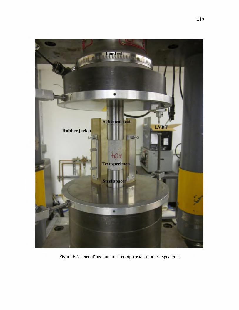
210

Figure E.3 Unconfined, uniaxial compression of a test specimen

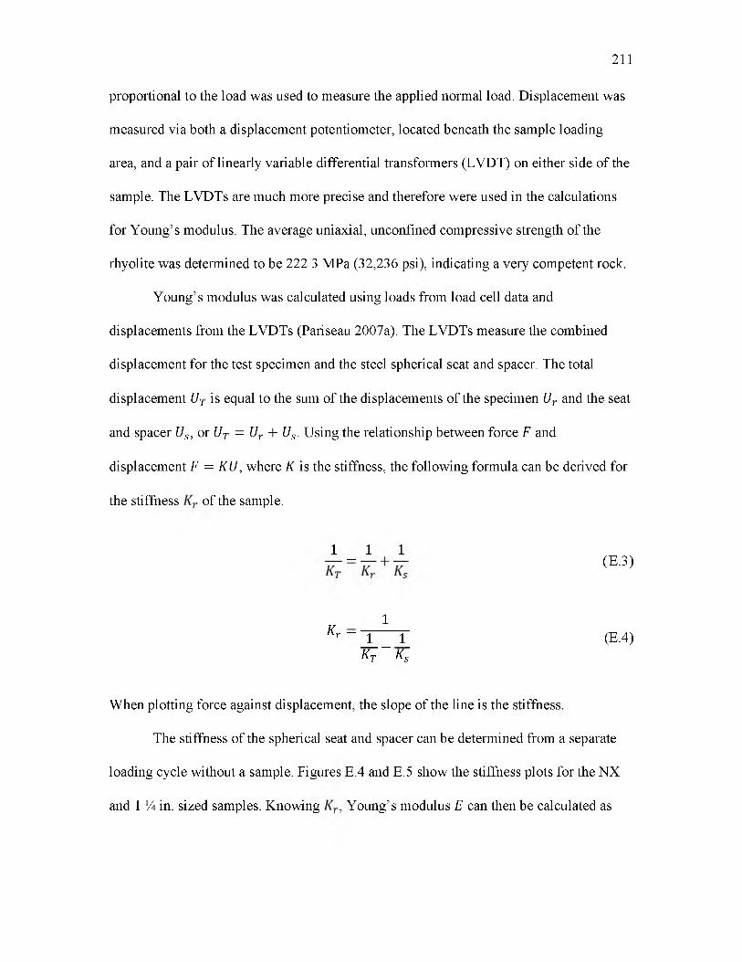
211

proportional to the load was used to measure the applied normal load. Displacement was

measured via both a displacement potentiometer, located beneath the sample loading

area, and a pair of linearly variable differential transformers (LVDT) on either side of the

sample. The LVDTs are much more precise and therefore were used in the calculations

for Young’s modulus. The average uniaxial, unconfined compressive strength of the

rhyolite was determined to be 222.3 MPa (32,236 psi), indicating a very competent rock.

Young’s modulus was calculated using loads from load cell data and

displacements from the LVDTs (Pariseau 2007a). The LVDTs measure the combined

displacement for the test specimen and the steel spherical seat and spacer. The total

displacement t/r is equal to the sum of the displacements of the specimen t/r and the seat

and spacer t/s, or t/r = t/r + t/s . Using the relationship between force F and

displacement F = fr^ , where K is the stiffness, the following formula can be derived for

the stiffness of the sample.

When plotting force against displacement, the slope of the line is the stiffness.

The stiffness of the spherical seat and spacer can be determined from a separate

loading cycle without a sample. Figures E.4 and E.5 show the stiffness plots for the NX

and 1 H in. sized samples. Knowing , Young’s modulus E can then be calculated as

1 _ 1 1( E.3)

1K r ~ J _ _ l _

Kr Ks(E.4)

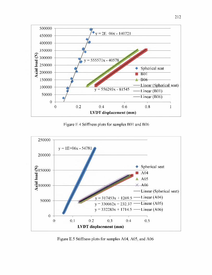
212

500000

450000

400000

350000

^ 300000 dola250000

•§ 200000

150000

100000

50000

0

y = 2E+06x - 140721

y = 555571x

Spherical seat B01

Linear (Spherical seat)y = 556293x - 81545 -L inear (B01)

Linear (B06)

01

0.2I 1

0.4 0.61

0.8 1LVDT displacement (mm)

Figure E.4 Stiffness plots for samples B01 and B06

250000

200000

N150000daoa

"h<

i100000

50000

y = 1E+06x - 54781

0.1 0.2 0.3 0.4LVDT displacement (mm)

♦ Spherical seat■ A04 A A05 X A06

y = 317453x + 1269.5

Linear (Spherical seat) -Linear (A04)

y = 330062x + 232.37 y = 332283x + 1714.5

-Linear (A05) Linear (A06)

0.50

0

Figure E.5 Stiffness plots for samples A04, A05, and A06

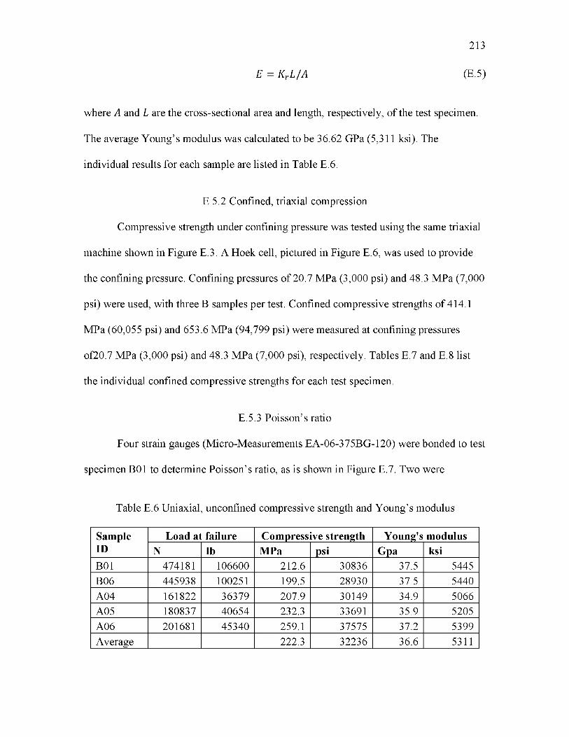
E = KrL/A (E.5)

213

where A and L are the cross-sectional area and length, respectively, of the test specimen.

The average Young’s modulus was calculated to be 36.62 GPa (5,311 ksi). The

individual results for each sample are listed in Table E.6.

E.5.2 Confined, triaxial compression

Compressive strength under confining pressure was tested using the same triaxial

machine shown in Figure E.3. A Hoek cell, pictured in Figure E.6, was used to provide

the confining pressure. Confining pressures of 20.7 MPa (3,000 psi) and 48.3 MPa (7,000

psi) were used, with three B samples per test. Confined compressive strengths of 414.1

MPa (60,055 psi) and 653.6 MPa (94,799 psi) were measured at confining pressures

of20.7 MPa (3,000 psi) and 48.3 MPa (7,000 psi), respectively. Tables E.7 and E.8 list

the individual confined compressive strengths for each test specimen.

E.5.3 Poisson’s ratio

Four strain gauges (Micro-Measurements EA-06-375BG-120) were bonded to test

specimen B01 to determine Poisson’s ratio, as is shown in Figure E.7. Two were

Table E.6 Uniaxial, unconfined compressive strength and Young’s modulus

SampleID

Load at failure Compressive strength Young's modulusN lb MPa psi Gpa ksi

B01 474181 106600 212.6 30836 37.5 5445B06 445938 100251 199.5 28930 37.5 5440A04 161822 36379 207.9 30149 34.9 5066A05 180837 40654 232.3 33691 35.9 5205A06 201681 45340 259.1 37575 37.2 5399Average 222.3 32236 36.6 5311

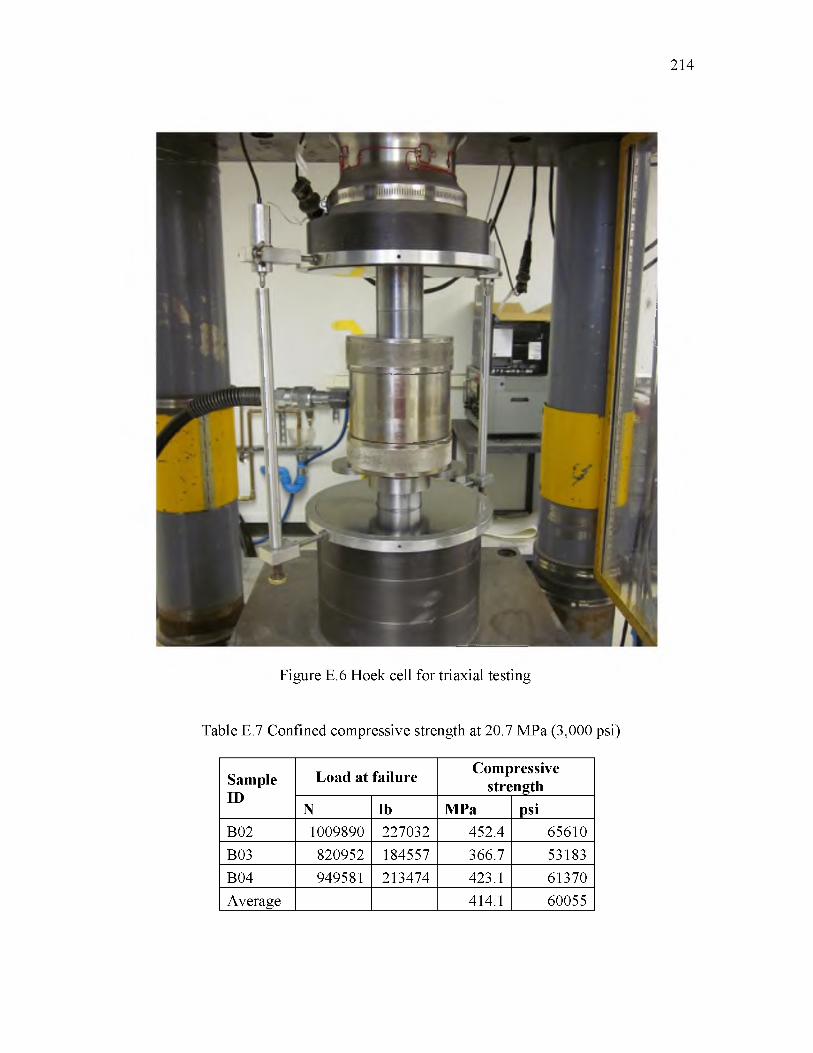
214

Figure E.6 Hoek cell for triaxial testing

Table E.7 Confined compressive strength at 20.7 MPa (3,000 psi)

SampleID

Load at failure Compressivestrength

N lb MPa psiB02 1009890 227032 452.4 65610B03 820952 184557 366.7 53183B04 949581 213474 423.1 61370Average 414.1 60055

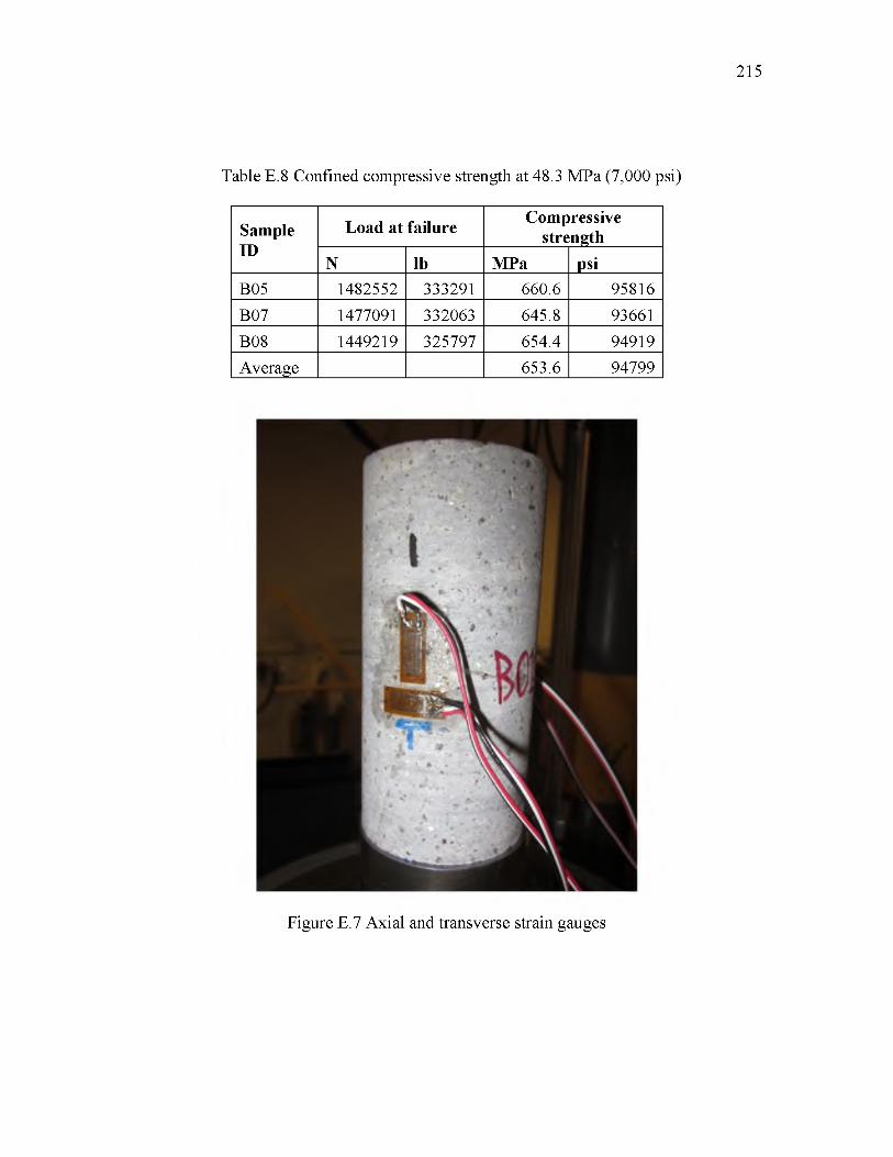
215

Table E.8 Confined compressive strength at 48.3 MPa (7,000 psi)

SampleID

Load at failure Compressivestrength

N lb MPa psiB05 1482552 333291 660.6 95816B07 1477091 332063 645.8 93661B08 1449219 325797 654.4 94919Average 653.6 94799

Figure E.7 Axial and transverse strain gauges

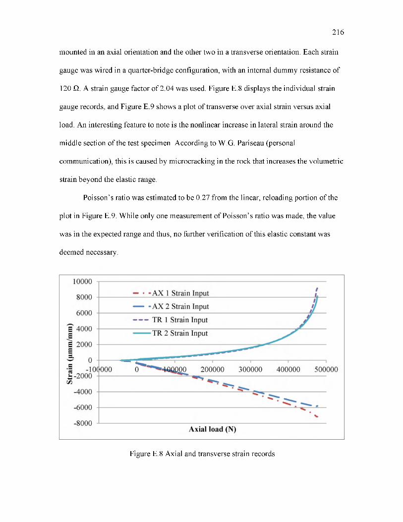
mounted in an axial orientation and the other two in a transverse orientation. Each strain

gauge was wired in a quarter-bridge configuration, with an internal dummy resistance of

120 Q. A strain gauge factor of 2.04 was used. Figure E.8 displays the individual strain

gauge records, and Figure E.9 shows a plot of transverse over axial strain versus axial

load. An interesting feature to note is the nonlinear increase in lateral strain around the

middle section of the test specimen. According to W.G. Pariseau (personal

communication), this is caused by microcracking in the rock that increases the volumetric

strain beyond the elastic range.

Poisson’s ratio was estimated to be 0.27 from the linear, reloading portion of the

plot in Figure E.9. While only one measurement of Poisson’s ratio was made, the value

was in the expected range and thus, no further verification of this elastic constant was

deemed necessary.

216

Figure E.8 Axial and transverse strain records

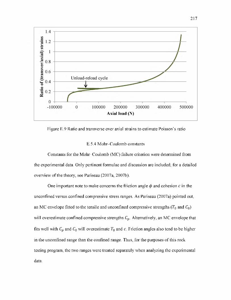
217

Axial load (N)

Figure E.9 Ratio and transverse over axial strains to estimate Poisson’s ratio

E.5.4 Mohr-Coulomb constants

Constants for the Mohr-Coulomb (MC) failure criterion were determined from

the experimental data. Only pertinent formulae and discussion are included; for a detailed

overview of the theory, see Pariseau (2007a, 2007b).

One important note to make concerns the friction angle and cohesion in the

unconfined versus confined compressive stress ranges. As Pariseau (2007a) pointed out,

an MC envelope fitted to the tensile and unconfined compressive strengths ( and )

will overestimate confined compressive strengths . Alternatively, an MC envelope that

fits well with and will overestimate and . Friction angles also tend to be higher

in the unconfined range than the confined range. Thus, for the purposes of this rock

testing program, the two ranges were treated separately when analyzing the experimental

data.

218

The MC failure envelope can by characterized by the equation (Pariseau 2007a,

2007b)

where t is the shear stress induced by the applied normal stress a. When fitting a linear

regression to the data, it is often easier to use the equation

where

am = (ai + a3)/T. is the applied mean normal stress that is also the center of a Mohr

circle when plotted in a — t stress space,

Tm = (a1 — a^) /2 is the deviatoric shear stress on the MC envelope directly above am,

a1 and a3 are the major and minor principal stresses for the given stress state,

0 is related to 0 such that tan 0 = sin 0 , and

k is related to c such that k = c cos 0.

MC constants 0 and c can be estimated for the unconfined compression range

from T0 and C0 (Pariseau 2007a):

For the confined compression range, linear regression was used to determine tan 0 and k,

which was then used to calculate 0 and c . The MC parameters estimated from

It I = a t a n 0 + c (E.6)

Tm = am tan 0 + k (E.7)

Cn — Tt( E.8)

( E.9)

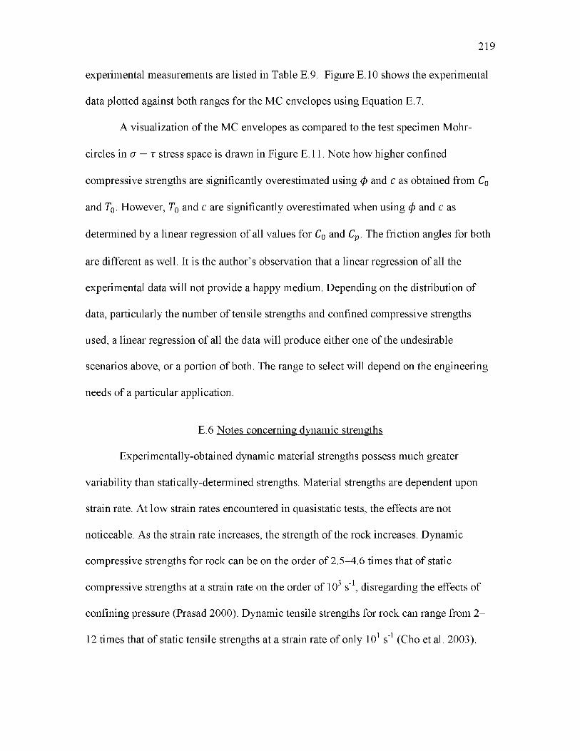
experimental measurements are listed in Table E.9. Figure E.10 shows the experimental

data plotted against both ranges for the MC envelopes using Equation E.7.

A visualization of the MC envelopes as compared to the test specimen Mohr-

circles in a — t stress space is drawn in Figure E.11. Note how higher confined

compressive strengths are significantly overestimated using 0 and c as obtained from C0

and T0. However, T0 and c are significantly overestimated when using 0 and c as

determined by a linear regression of all values for C0 and Cp. The friction angles for both

are different as well. It is the author’s observation that a linear regression of all the

experimental data will not provide a happy medium. Depending on the distribution of

data, particularly the number of tensile strengths and confined compressive strengths

used, a linear regression of all the data will produce either one of the undesirable

scenarios above, or a portion of both. The range to select will depend on the engineering

needs of a particular application.

E.6 Notes concerning dynamic strengths

Experimentally-obtained dynamic material strengths possess much greater

variability than statically-determined strengths. Material strengths are dependent upon

strain rate. At low strain rates encountered in quasistatic tests, the effects are not

noticeable. As the strain rate increases, the strength of the rock increases. Dynamic

compressive strengths for rock can be on the order of 2.5-4.6 times that of static

3 1compressive strengths at a strain rate on the order of 10 s- , disregarding the effects of

confining pressure (Prasad 2000). Dynamic tensile strengths for rock can range from 2­

12 times that of static tensile strengths at a strain rate of only 101 s-1 (Cho et al. 2003).

219

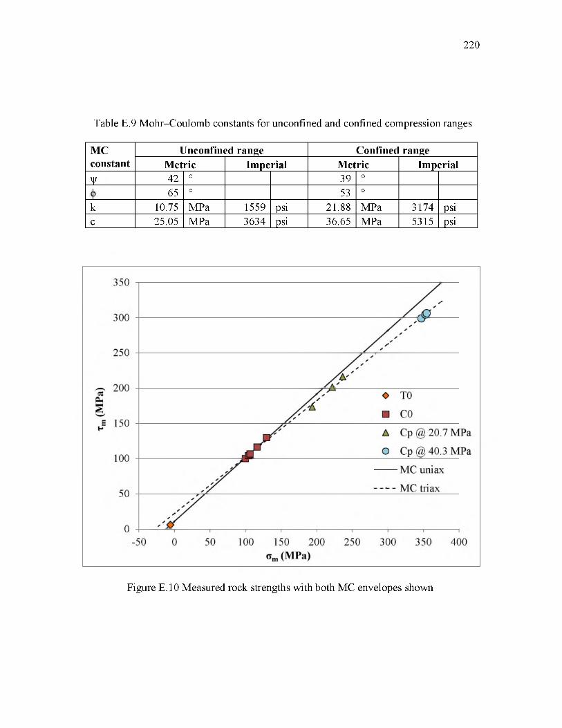
220

Table E.9 Mohr-Coulomb constants for unconfined and confined compression ranges

MCconstant

Unconfined range Confinet rangeMetric Imperial Metric Imperial

¥ 42 O 39 O

65 O 53 O

k 10.75 MPa 1559 psi 21.88 MPa 3174 psic 25.05 MPa 3634 psi 36.65 MPa 5315 psi

Figure E.10 Measured rock strengths with both MC envelopes shown

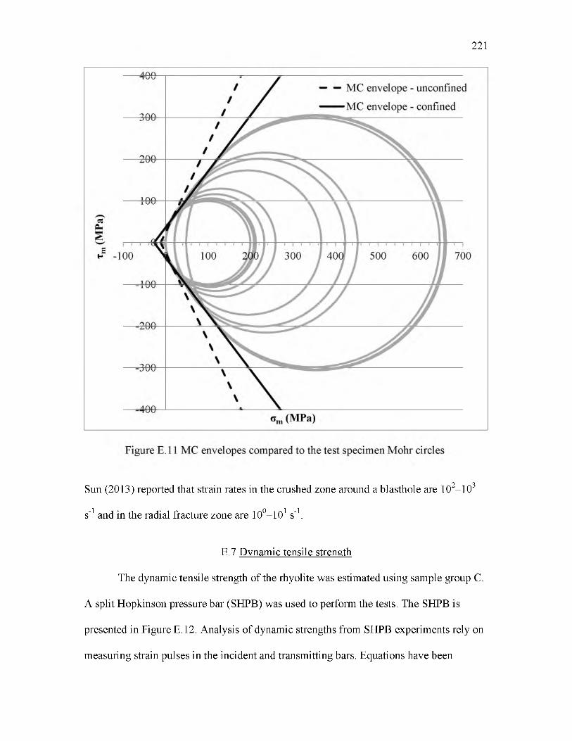
221

2 3Sun (2013) reported that strain rates in the crushed zone around a blasthole are 1 0 -1 0

s-1 and in the radial fracture zone are 100-1 0 1 s-1.

E.7 Dynamic tensile strength

The dynamic tensile strength of the rhyolite was estimated using sample group C.

A split Hopkinson pressure bar (SHPB) was used to perform the tests. The SHPB is

presented in Figure E.12. Analysis of dynamic strengths from SHPB experiments rely on

measuring strain pulses in the incident and transmitting bars. Equations have been

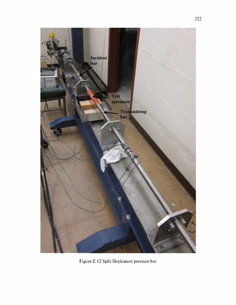
222

Figure E.12 Split Hopkinson pressure bar

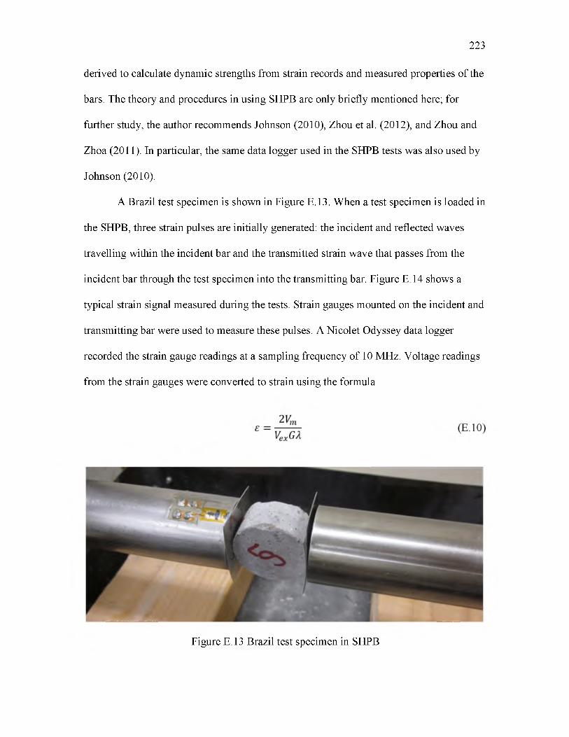
derived to calculate dynamic strengths from strain records and measured properties of the

bars. The theory and procedures in using SHPB are only briefly mentioned here; for

further study, the author recommends Johnson (2010), Zhou et al. (2012), and Zhou and

Zhoa (2011). In particular, the same data logger used in the SHPB tests was also used by

Johnson (2010).

A Brazil test specimen is shown in Figure E.13. When a test specimen is loaded in

the SHPB, three strain pulses are initially generated: the incident and reflected waves

travelling within the incident bar and the transmitted strain wave that passes from the

incident bar through the test specimen into the transmitting bar. Figure E. 14 shows a

typical strain signal measured during the tests. Strain gauges mounted on the incident and

transmitting bar were used to measure these pulses. A Nicolet Odyssey data logger

recorded the strain gauge readings at a sampling frequency of 10 MHz. Voltage readings

from the strain gauges were converted to strain using the formula

223

Figure E.13 Brazil test specimen in SHPB

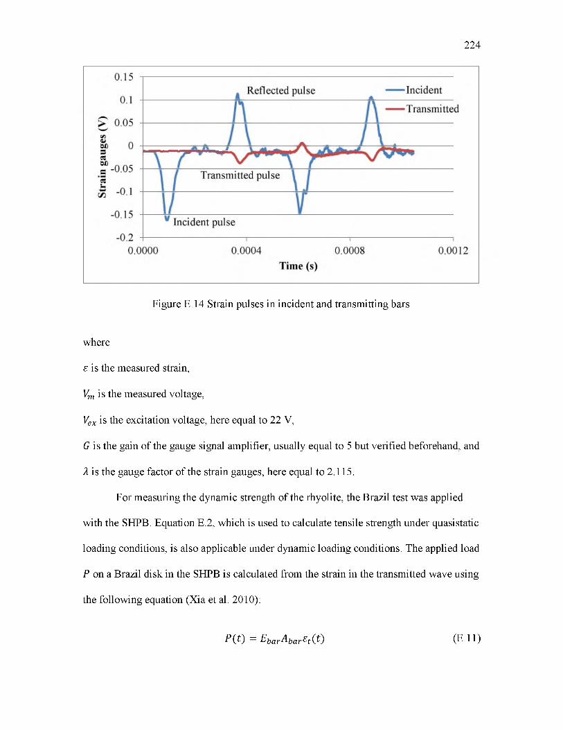
224

Figure E.14 Strain pulses in incident and transmitting bars

where

£ is the measured strain,

Vm is the measured voltage,

Vex is the excitation voltage, here equal to 22 V,

G is the gain of the gauge signal amplifier, usually equal to 5 but verified beforehand, and

A is the gauge factor of the strain gauges, here equal to 2.115.

For measuring the dynamic strength of the rhyolite, the Brazil test was applied

with the SHPB. Equation E.2, which is used to calculate tensile strength under quasistatic

loading conditions, is also applicable under dynamic loading conditions. The applied load

P on a Brazil disk in the SHPB is calculated from the strain in the transmitted wave using

the following equation (Xia et al. 2010):

P ( t ) = EbarAbar£t ( t) (E.11)

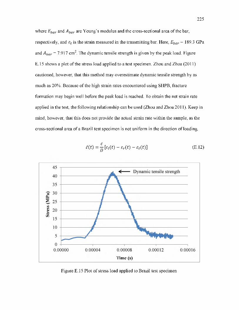
where Ebar and Abar are Young’s modulus and the cross-sectional area of the bar,

respectively, and £t is the strain measured in the transmitting bar. Here, Ebar = 189.3 GPa

and A bar = 7.917 cm2. The dynamic tensile strength is given by the peak load. Figure

E.15 shows a plot of the stress load applied to a test specimen. Zhou and Zhoa (2011)

cautioned, however, that this method may overestimate dynamic tensile strength by as

much as 20%. Because of the high strain rates encountered using SHPB, fracture

formation may begin well before the peak load is reached. To obtain the net strain rate

applied in the test, the following relationship can be used (Zhou and Zhoa 2011). Keep in

mind, however, that this does not provide the actual strain rate within the sample, as the

cross-sectional area of a Brazil test specimen is not uniform in the direction of loading.

£ ( 0 = ^ [£ ( 0 - £r ( 0 - £t ( 0 ] (E12)

225

Time (s)

Figure E.15 Plot of stress load applied to Brazil test specimen

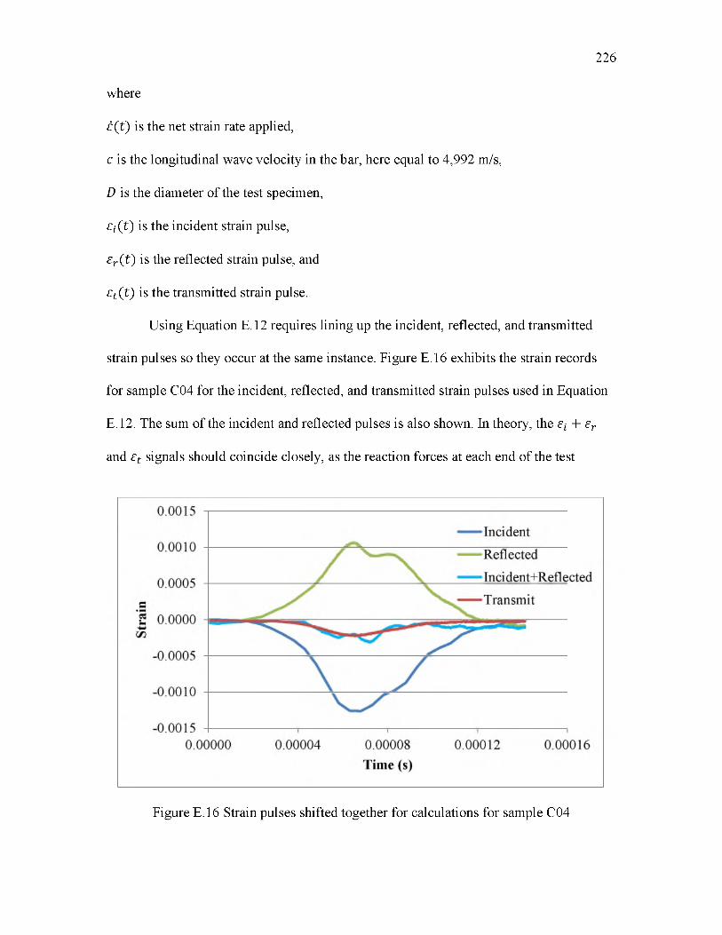
where

E(t) is the net strain rate applied,

c is the longitudinal wave velocity in the bar, here equal to 4,992 m/s,

D is the diameter of the test specimen,

Et( t) is the incident strain pulse,

Er (t) is the reflected strain pulse, and

Et (t) is the transmitted strain pulse.

Using Equation E. 12 requires lining up the incident, reflected, and transmitted

strain pulses so they occur at the same instance. Figure E.16 exhibits the strain records

for sample C04 for the incident, reflected, and transmitted strain pulses used in Equation

E.12. The sum of the incident and reflected pulses is also shown. In theory, the Et + Er

and Et signals should coincide closely, as the reaction forces at each end of the test

226

Figure E.16 Strain pulses shifted together for calculations for sample C04

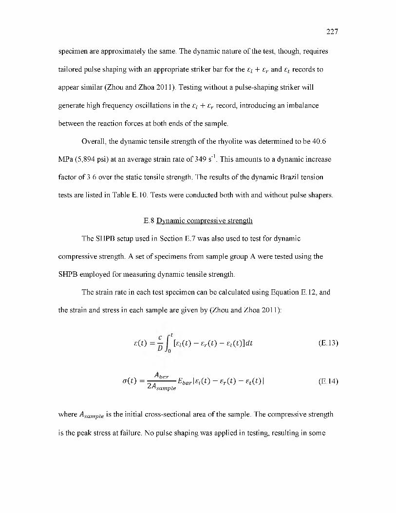
specimen are approximately the same. The dynamic nature of the test, though, requires

tailored pulse shaping with an appropriate striker bar for the £* + £r and £t records to

appear similar (Zhou and Zhoa 2011). Testing without a pulse-shaping striker will

generate high frequency oscillations in the £* + £r record, introducing an imbalance

between the reaction forces at both ends of the sample.

Overall, the dynamic tensile strength of the rhyolite was determined to be 40.6

MPa (5,894 psi) at an average strain rate of 349 s-1. This amounts to a dynamic increase

factor of 3.6 over the static tensile strength. The results of the dynamic Brazil tension

tests are listed in Table E.10. Tests were conducted both with and without pulse shapers.

E.8 Dynamic compressive strength

The SHPB setup used in Section E.7 was also used to test for dynamic

compressive strength. A set of specimens from sample group A were tested using the

SHPB employed for measuring dynamic tensile strength.

The strain rate in each test specimen can be calculated using Equation E. 12, and

the strain and stress in each sample are given by (Zhou and Zhoa 2011):

£(0 = [£*(t) - £r (t) - £t ( t) ]d t (E.13)

^ J-t f f y

a ( t ) = T l -------- ^ [ £ * ( 0 - £ r(0 - £t ( 0 ] (E.14)^•^sampie

where ^ sampie is the initial cross-sectional area of the sample. The compressive strength

is the peak stress at failure. No pulse shaping was applied in testing, resulting in some

227

228

Table E.10 Dynamic tensile strengths - group C

SampleID

Tensile strength Dynamic increase factor

Peak strain rate

MPa psi s-1C03 37.35 5417 3.3 351C04 42.52 6168 3.8 334C05 37.22 5398 3.3 358C06 33.81 4903 3.0 358C07 35.35 5128 3.1 325C08 41.74 6054 3.7 320C09 34.87 5057 3.1 290C10 35.54 5155 3.1 324C11 43.31 6282 3.8 363C12 36.05 5228 3.2 280C13 36.06 5230 3.2 279C14 38.31 5557 3.4 292C15 42.18 6117 3.7 289C16 39.32 5703 3.5 289C17 39.68 5755 3.5 378C18* 45.93 6662 4.1 444C19* 52.47 7609 4.6 445C20* 50.83 7372 4.5 465C21* 49.59 7192 4.4 439Average 40.64 5894 3.6 349* No pulse shaper used

unbalanced loading at both ends of the specimen and high-frequency strain components.

Figure E.17 shows the superimposed strain records for one of the samples.

The results of the tests are listed in Table E.11. The average dynamic compressive

strength of the rhyolite was determined to be 301.6 MPa (43,740 psi), which gives a

dynamic increase factor of 1.4 times greater than the static compressive strength. The

average strain rate for these tests was 285 s-1. Samples that failed from tensile spalling

were not included in the final results, but are listed in Table E.11.

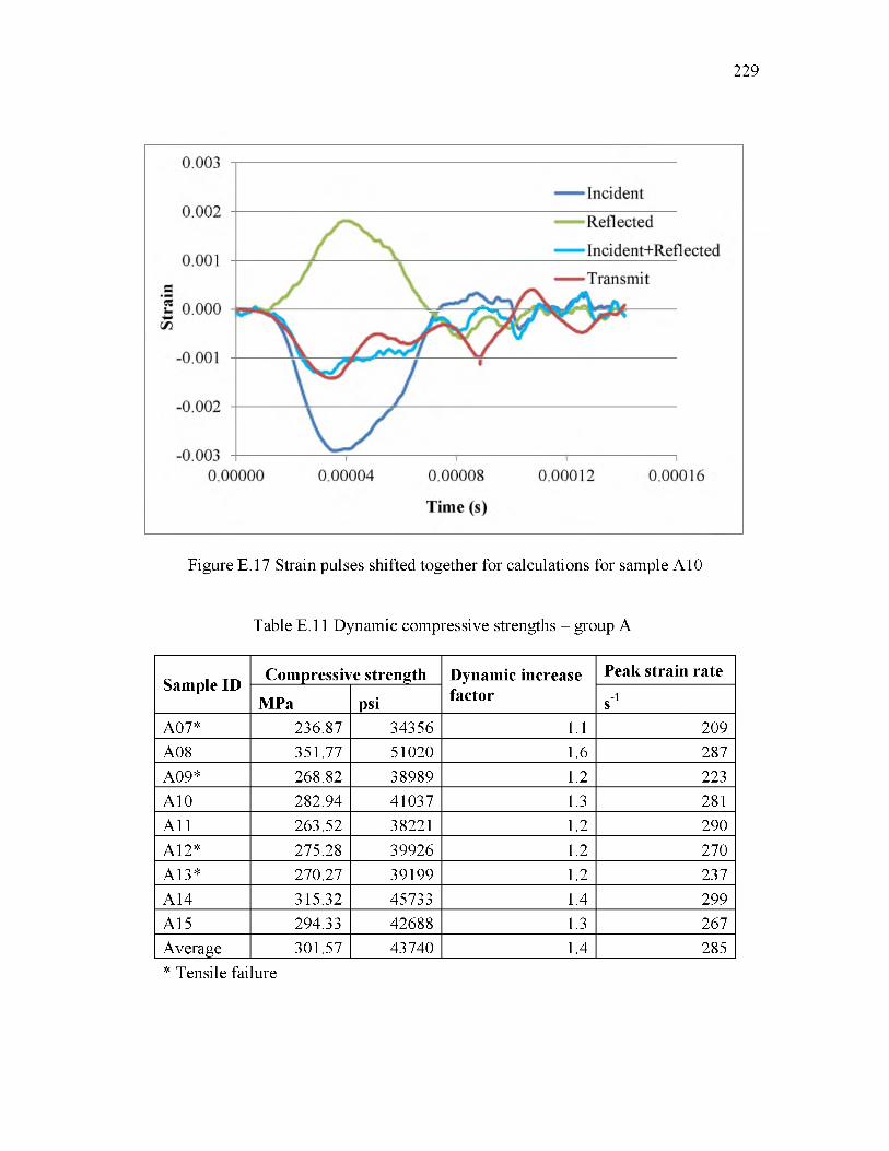
229

Figure E.17 Strain pulses shifted together for calculations for sample A10

Table E.11 Dynamic compressive strengths - group A

Sample ID Compressive strength Dynamic increase factor

Peak strain rate

MPa psi s-1A07* 236.87 34356 1.1 209A08 351.77 51020 1.6 287A09* 268.82 38989 1.2 223A10 282.94 41037 1.3 281A11 263.52 38221 1.2 290A12* 275.28 39926 1.2 270A13* 270.27 39199 1.2 237A14 315.32 45733 1.4 299A15 294.33 42688 1.3 267Average 301.57 43740 1.4 285* Tensile failure

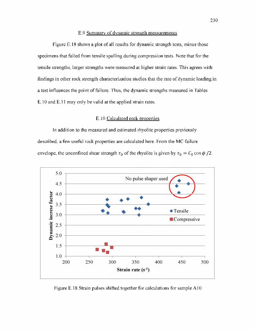
230

E.9 Summary of dynamic strength measurements

Figure E.18 shows a plot of all results for dynamic strength tests, minus those

specimens that failed from tensile spalling during compression tests. Note that for the

tensile strengths, larger strengths were measured at higher strain rates. This agrees with

findings in other rock strength characterization studies that the rate of dynamic loading in

a test influences the point of failure. Thus, the dynamic strengths measured in Tables

E.10 and E.11 may only be valid at the applied strain rates.

E.10 Calculated rock properties

In addition to the measured and estimated rhyolite properties previously

described, a few useful rock properties are calculated here. From the MC failure

envelope, the unconfined shear strength t0 of the rhyolite is given by t0 = C0 cos 0 /2.

Figure E.18 Strain pulses shifted together for calculations for sample A10

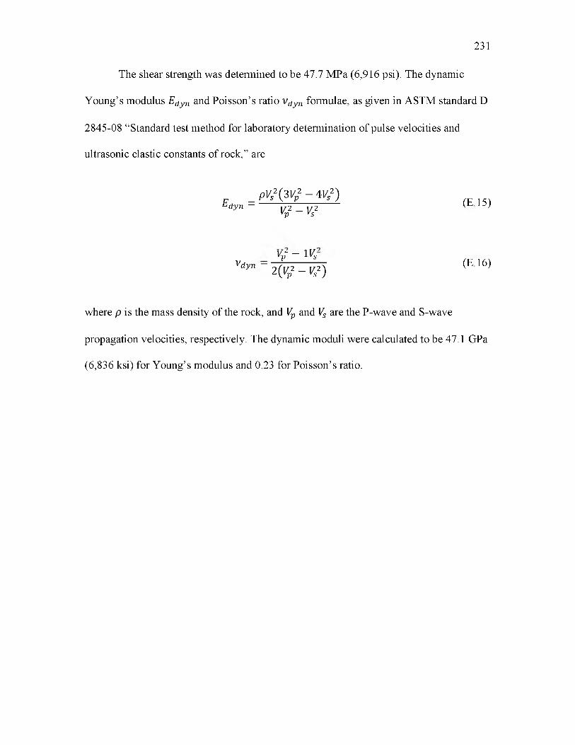
The shear strength was determined to be 47.7 MPa (6,916 psi). The dynamic

Young’s modulus Edyn and Poisson’s ratio v dyn formulae, as given in ASTM standard D

2845-08 “Standard test method for laboratory determination of pulse velocities and

ultrasonic elastic constants of rock,” are

231

P Vs2( 3 Vv2 - 4 Vs2 )E*yn = P ^ - v f s > (E15)

V - IKv“yn = 2(V„2 - Vs2) (E16)

where p is the mass density of the rock, and Vv and Vs are the P-wave and S-wave

propagation velocities, respectively. The dynamic moduli were calculated to be 47.1 GPa

(6,836 ksi) for Young’s modulus and 0.23 for Poisson’s ratio.

APPENDIX F

PYTHON CODE FOR HOLMBERG-PERSSON

MODEL

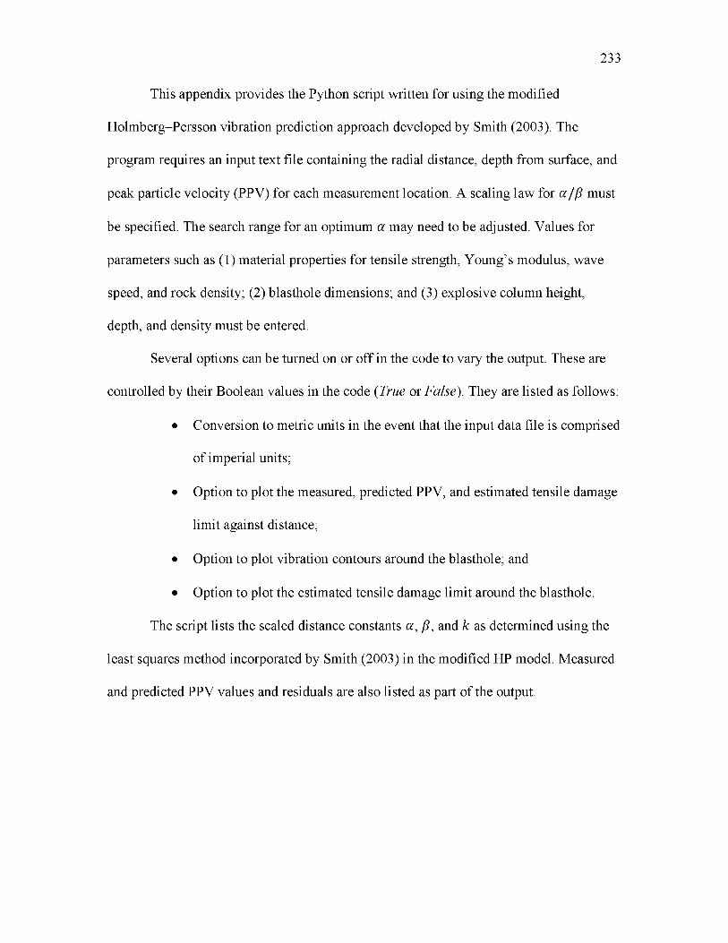
This appendix provides the Python script written for using the modified

Holmberg-Persson vibration prediction approach developed by Smith (2003). The

program requires an input text file containing the radial distance, depth from surface, and

peak particle velocity (PPV) for each measurement location. A scaling law for a / ^ must

be specified. The search range for an optimum a may need to be adjusted. Values for

parameters such as (1) material properties for tensile strength, Young’s modulus, wave

speed, and rock density; (2) blasthole dimensions; and (3) explosive column height,

depth, and density must be entered.

Several options can be turned on or off in the code to vary the output. These are

controlled by their Boolean values in the code (True or False). They are listed as follows:

• Conversion to metric units in the event that the input data file is comprised

of imperial units;

• Option to plot the measured, predicted PPV, and estimated tensile damage

limit against distance;

• Option to plot vibration contours around the blasthole; and

• Option to plot the estimated tensile damage limit around the blasthole.

The script lists the scaled distance constants a , ^ , and k as determined using the

least squares method incorporated by Smith (2003) in the modified HP model. Measured

and predicted PPV values and residuals are also listed as part of the output.

233

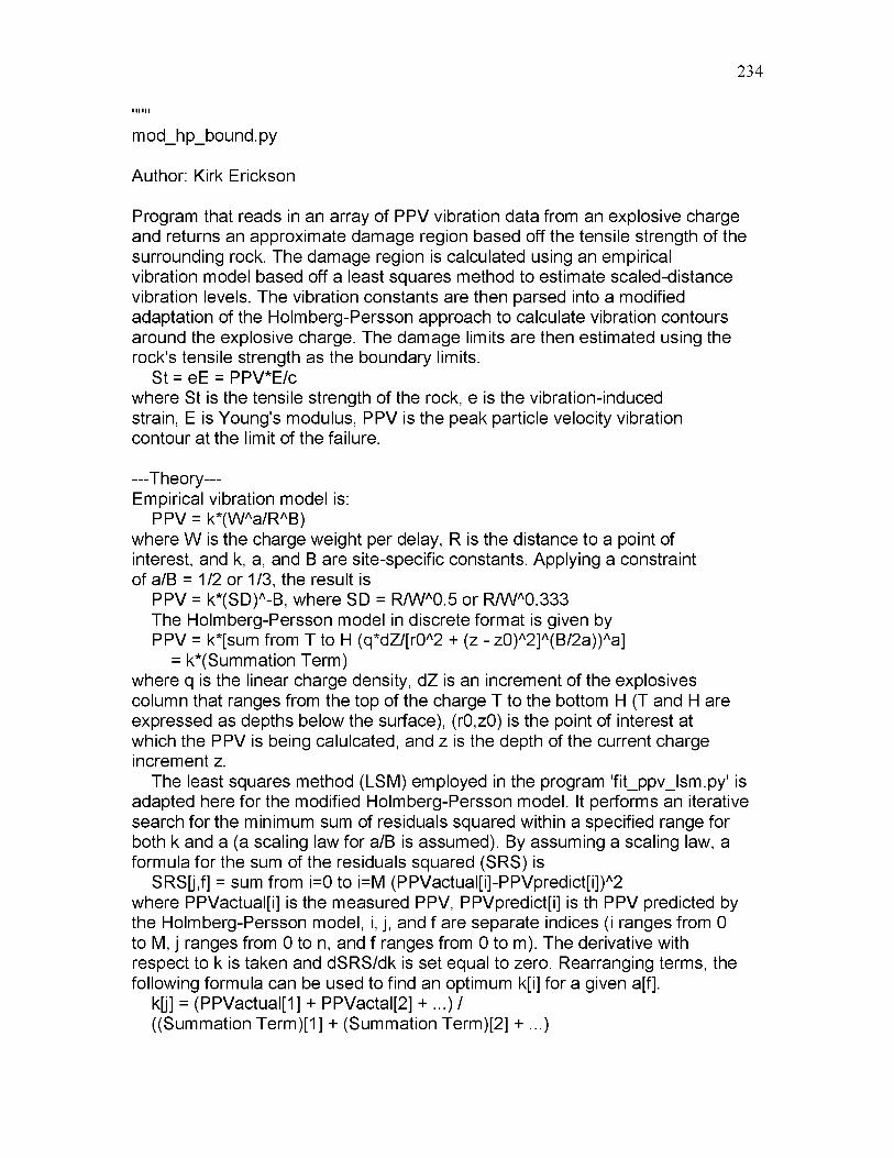
234

I H H !

mod_hp_bound.py

Author: Kirk Erickson

Program that reads in an array of PPV vibration data from an explosive charge and returns an approximate damage region based off the tensile strength of the surrounding rock. The damage region is calculated using an empirical vibration model based off a least squares method to estimate scaled-distance vibration levels. The vibration constants are then parsed into a modified adaptation of the Holmberg-Persson approach to calculate vibration contours around the explosive charge. The damage limits are then estimated using the rock's tensile strength as the boundary limits.

St = eE = PPV*E/c where St is the tensile strength of the rock, e is the vibration-induced strain, E is Young's modulus, PPV is the peak particle velocity vibration contour at the limit of the failure.

---Theory---Empirical vibration model is:

PPV = k*(WAa/RAB) where W is the charge weight per delay, R is the distance to a point of interest, and k, a, and B are site-specific constants. Applying a constraint of a/B = 1/2 or 1/3, the result is

PPV = k*(SD)A-B, where SD = R/WA0.5 or R/WA0.333 The Holmberg-Persson model in discrete format is given by PPV = k*[sum from T to H (q*dZ/[r0A2 + (z - z0)A2]A(B/2a))Aa]

= k*(Summation Term) where q is the linear charge density, dZ is an increment of the explosives column that ranges from the top of the charge T to the bottom H (T and H are expressed as depths below the surface), (r0,z0) is the point of interest at which the PPV is being calulcated, and z is the depth of the current charge increment z.

The least squares method (LSM) employed in the program 'fit_ppv_lsm.py' is adapted here for the modified Holmberg-Persson model. It performs an iterative search for the minimum sum of residuals squared within a specified range for both k and a (a scaling law for a/B is assumed). By assuming a scaling law, a formula for the sum of the residuals squared (SRS) is

SRS[j,f] = sum from i=0 to i=M (PPVactual[i]-PPVpredict[i])A2 where PPVactual[i] is the measured PPV, PPVpredict[i] is th PPV predicted by the Holmberg-Persson model, i, j, and f are separate indices (i ranges from 0 to M, j ranges from 0 to n, and f ranges from 0 to m). The derivative with respect to k is taken and dSRS/dk is set equal to zero. Rearranging terms, the following formula can be used to find an optimum k[i] for a given a[f].

k[j] = (PPVactual[1] + PPVactal[2] + ...) /((Summation Term)[1] + (Summation Term)[2] + ...)

235

Note: Empirical least squares vibration algortihm and the modified Holmberg- Persson model was originally developed by Amanda Ann Smith, M.S. thesis published at the University of Utah titled "A Modified Holmberg-Persson Approach to Predict Blast Damage" (2003)

''' To run code, first set working directory using os.chdir() command, then execute file using execfile() command.'''# os.chdir('C:\Users\Kirk\U of U\M.S. thesis\Numerical simulations\Modified HP model')# execfile('mod_hp_bound.py')

# Import modules import numpy as npimport matplotlib.pyplot as plt

# Import data file'''Imported data file requires 3 columns: radial distance to blasthole, depthas measured from blasthole collar, and peak particle velocity. Program assumes1 row of headerlines (column labels). No conversion between units is made.Progam written for units of either ft and ips or m and mm/s.'''h_lines = 1 # Number of lines at beginning of file to skipf_dir = 'C:\Users\Kirk\U of U\M.S. thesis\Numerical simulations\Modified HPmodel\\'filename = f_dir + 'br_data.txt'R = np.loadtxt(filename,skiprows = h_lines)[:,0] # radial distance from blasthole Z = np.loadtxt(filename,skiprows = h_lines)[:,1] # depth measured from collar PPV = np.loadtxt(filename,skiprows = h_lines)[:,2] # measured PPV N = np.size(R)

# Material propertiesSt = 1638 # Tensile strength in psi - can be static or dynamic E = 5311 # Young's modulus is ksi c = 15111 # Wave velocity in ft/s - usually P-wave velocity units_metric = False # Inform program if input units are metric or imperial conv_to_m = True # Convert to metric units of m, Pa, mm/s, kg

# Blasthole parametersd = 4.75 # Blasthole diameter, inchesd = d/12 # Blasthole diamater, ftH = 22. # Depth of blasthole, ftT = 14. # Stemming height, ftLe = H - T # Length of explosive columnpe = 0.85 # Specific gravity of explosivewg = 62.43 # weight/volume of water, here lb/ftA3

236

q = pe*d**2.*wg*np.pi/4. # Charge density in blasthole, lb/ft

# Conversion to metric units ft_to_m = 0.3048 in_to_mm = 25.4 psi_to_pa = 6894.757 lbm_to_kg = 0.4535924

if conv_to_m:R *= ft_to_m # ft to m Z *= ft_to_mPPV *= in_to_mm # in./s to mm/s St *= psi_to_pa*10**-6 # psi to MPa E *= psi_to_pa*10**-6 # ksi to GPa c *= ft_to_m d *= ft_to_m H *= ft_to_m T *= ft_to_m Le *= ft_to_mwg *= lbm_to_kg/ft_to_m**3 # lb/ftA3 to g/cmA3 q *= lbm_to_kg/ft_to_m # lb/ft to kg/m

del(ft_to_m ,in_to_mm,psi_to_pa,lbm_to_kg)

# Input parameters for vibration modelsc_law = 0.333 # scaling law; equal to a/Ba_min = 0.3 a_max = 2.0a_inc = 0.001 # number of iterations to perform for aa_itr = np.int(np.round((a_max - a_min)/a_inc))# increment to advance a in calculations

# Plotting parametersdisp_PPV = True # Plot comparison of measured and predicted PPV disp_vb = True # Display vibration contours disp_lim = True # Display damage limits based off tensile strength ext_factor = 0.2r_max = 40*d*(1+ext_factor) # Estimated radial extent of damage limit to plot

# Define function for calculating summation term in Holmberg-Persson model def hpsum(R,Z,PPV,d,q,dZ,num_dz,sZ,a,sc_law):

'''Note: Function assumes that the length of the explosive charge is comprised of an integer number num_dz of charge increments dZ.Input arguments are:

R - array of radial distances from blasthole Z - depths measured from collar

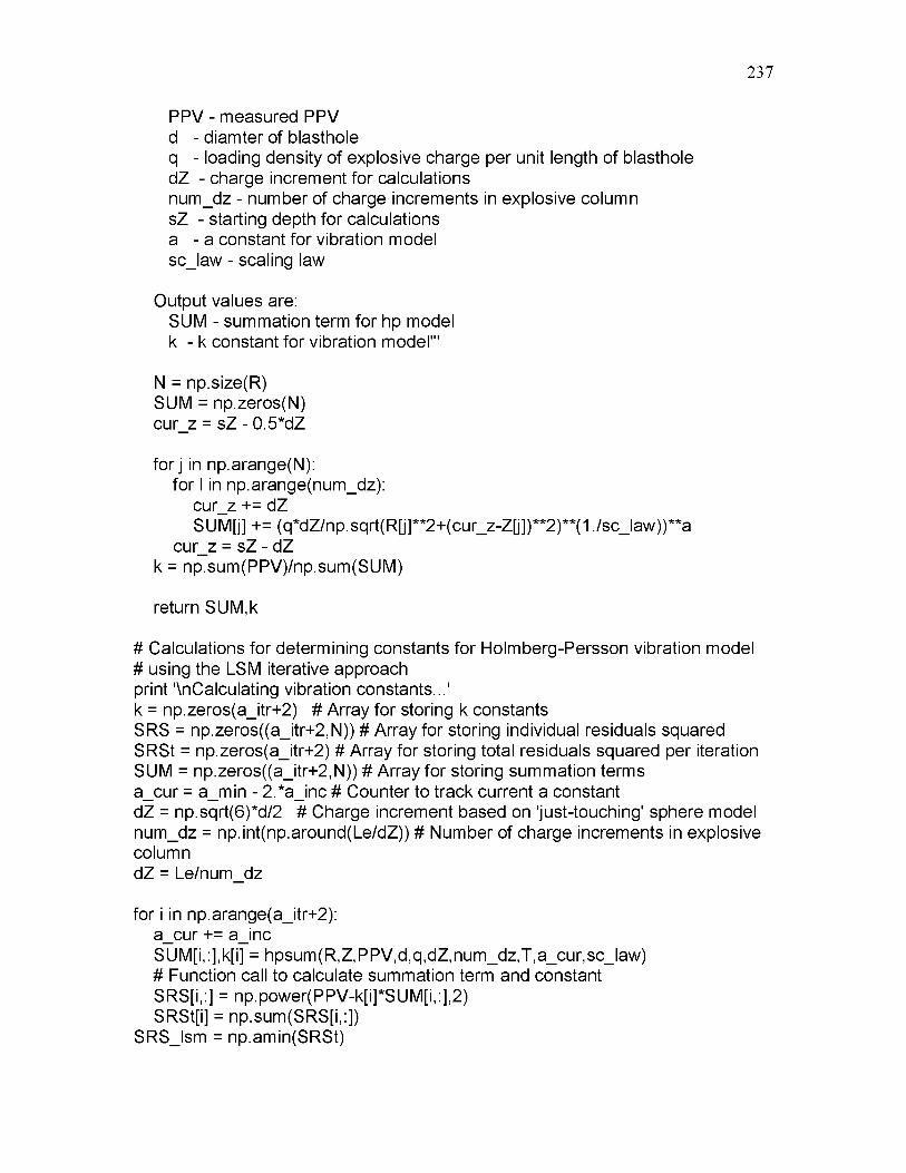
237

PPV - measured PPV d - diamter of blastholeq - loading density of explosive charge per unit length of blastholedZ - charge increment for calculationsnum_dz - number of charge increments in explosive columnsZ - starting depth for calculationsa - a constant for vibration modelsc_law - scaling law

Output values are:SUM - summation term for hp model k - k constant for vibration model'''

N = np.size(R)SUM = np.zeros(N) cur_z = sZ - 0.5*dZ

for j in np.arange(N):for l in np.arange(num_dz):

cur_z += dZSUM[j] += (q*dZ/np.sqrt(R0r*2+(cur_z-ZG])**2)**(l/scJaw))**a

cur_z = sZ - dZ k = np.sum(PPV)/np.sum(SUM)

return SUM,k

# Calculations for determining constants for Holmberg-Persson vibration model# using the LSM iterative approach print '\nCalculating vibration constants...'k = np.zeros(a_itr+2) # Array for storing k constantsSRS = np.zeros((a_itr+2,N)) # Array for storing individual residuals squaredSRSt = np.zeros(a_itr+2) # Array for storing total residuals squared per iterationSUM = np.zeros((a_itr+2,N)) # Array for storing summation termsa_cur = a_min - 2.*a_inc # Counter to track current a constantdZ = np.sqrt(6)*d/2 # Charge increment based on 'just-touching' sphere modelnum_dz = np.int(np.around(Le/dZ)) # Number of charge increments in explosivecolumndZ = Le/num_dz

for i in np.arange(a_itr+2): a_cur += a_incSUM[i,:],k[i] = hpsum(R,Z,PPV,d,q,dZ,num_dz,T,a_cur,sc_law)# Function call to calculate summation term and constant SRS[i,:] = np.power(PPV-k[i]*SUM[i,:],2)SRSt[i] = np.sum(SRS[i,:])

SRS_lsm = np.amin(SRSt)

238

mindex = np.argmin(SRSt)-1 a_lsm = a_min + a_inc*mindex k_lsm = k[mindex]SUM = SUM[mindex,:] if a_lsm<a_min or a_lsm>a_max:

print '\nOptimum detected outside of specified limits!\n'

# Print resultsprint '\nHolmberg-Persson vibration model constants'print 'Scaling law a/B = {:5.3f}'.format(sc_law)print 'Constant\tValue \t'print 'a \t{0:>8.3f}\t'.format(a_lsm)print 'k \t{0:>7.2f}\t'.format(k_lsm)print 'SRS \t{0:>8.3f}\t'.format(SRS_lsm)

# Calcute vibration contour limitsif units_metric or (not(units_metric) and conv_to_m):

PPV_lim = St*c/E # PPV in mm/sprint'\nPPV limit for tensile failure is {:>0.0f} mm/s'.format(PPV_lim)

else:PPV_lim = St*c/E*12/1000. # PPV in ipsprint'\nPPV limit for tensile failure is {:>0.1f} ips'.format(PPV_lim)

# Calculate and plot actual vs predicted PPV PPV_pred = k_lsm*SUMrsd = PPV - PPV_predif units_metric or (not(units_metric) and conv_to_m):

print '\nPPV in mm/s are as follows:' print 'PPV actual PPV predicted Residuals' for i in np.arange(N):

print '{0:>10.0f} {1:>13.0f} {2:>9.0f}'.format(PPV[i],PPV_pred[i],\ rsd[i])

else:print '\nPPV in ips are as follows:'print 'PPV actual PPV predicted Residuals'for i in np.arange(N):

print '{0:>8.1f} {1:>11.1f} {2:>7.1f}'.format(PPV[i],PPV_pred[i],\ rsd[i])

if disp_PPV:D = np.sqrt(np.power(R,2)+np.power(T+0.5*Le,2)) plt.hold(True) # Toggle hold on for multiply plot commands plt.plot(D,PPV,'ms',D,PPV_pred,'cv',markersize=8,zorder=2) # Plot PPV

valuespaxis = np.asarray(plt.axis()) # Axes extents D_range = np.amax(D) - np.amin(D)

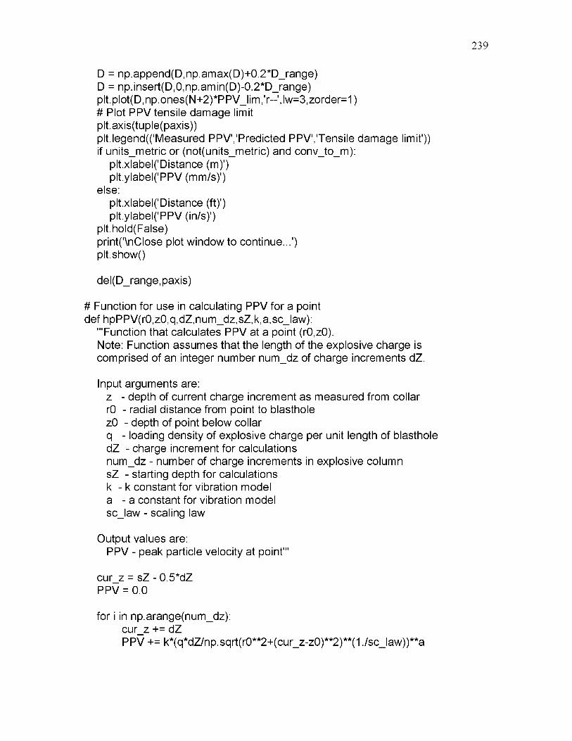
239

D = np.append(D,np.amax(D)+0.2*D_range)D = np.insert(D,0,np.amin(D)-0.2*D_range) plt.plot(D,np.ones(N+2)*PPV_lim,'r--',lw=3,zorder=1)# Plot PPV tensile damage limit plt.axis(tuple(paxis))plt.legend(('Measured PPV','Predicted PPV','Tensile damage limit')) if units_metric or (not(units_metric) and conv_to_m):

plt.xlabel('Distance (m)') plt.ylabel('PPV (mm/s)')

else:plt.xlabel('Distance (ft)') plt.ylabel('PPV (in/s)')

plt.hold(False)print('\nClose plot window to continue...') plt.show()

del(D_range,paxis)

# Function for use in calculating PPV for a point def hpPPV(r0,z0,q,dZ,num_dz,sZ,k,a,sc_law):

'''Function that calculates PPV at a point (r0,z0).Note: Function assumes that the length of the explosive charge is comprised of an integer number num_dz of charge increments dZ.

Input arguments are: z - depth of current charge increment as measured from collar r0 - radial distance from point to blasthole z0 - depth of point below collarq - loading density of explosive charge per unit length of blastholedZ - charge increment for calculationsnum_dz - number of charge increments in explosive columnsZ - starting depth for calculationsk - k constant for vibration modela - a constant for vibration modelsc_law - scaling law

Output values are:PPV - peak particle velocity at point'''

cur_z = sZ - 0.5*dZ PPV = 0.0

for i in np.arange(num_dz): cur_z += dZPPV += k*(q*dZ/np.sqrt(r0**2+(cur_z-z0)**2)**(1 ./sc_law))**a

240

return PPV

# Generate vibration contour grid - origin taken through borehole axis print '\nGenerating vibration contour grid...'dx = d/4 # Nominal grid spacings dy = d/4num_dx = np.int(np.ceil(0.8*r_max/dx)) # spacing on either side of blasthole num_dy = np.int(np.ceil((H+r_max/1.5)/dy)) # spacing below blasthole DX = num_dx*dx # Grid extents DY = num_dy*dygvib = np.zeros((num_dy,2*num_dx-1)) # PPV vibration grid, laid out so rows# correspond with y-direction and columns with x-direction xvib = np.linspace(-DX,DX,2*num_dx-1)yvib = np.linspace(0.0,DY,num_dy)ind_top = np.int(np.floor(T/dy)) # Index for grid point directly above blasthole ind_bot = np.int(np.ceil(H/dy)) # Index for grid point directly below blasthole

cur_x = -dx cur_y = -dy

for i in np.arange(0,ind_top): # Start calculations at top of model cur_y += dyfor j in (np.arange(num_dx)+num_dx-1): # Start calculations at center of model

cur_x += dxgvib[i,j] = hpPPV(cur_x,cur_y,q,dZ,num_dz,T,k_lsm,a_lsm,sc_law)

cur_x = -dx

cur_x = 0 x_skip = 0 while cur_x < d/2:

cur_x += dx x_skip += 1

cur_x_temp = cur_x

cur_x -= dx

for i in np.arange(ind_top,ind_bot): cur_y += dyfor j in (np.arange(num_dx-x_skip)+num_dx+x_skip-1):

cur_x += dxgvib[i,j] = hpPPV(cur_x,cur_y,q,dZ,num_dz,T,k_lsm,a_lsm,sc_law)

cur_x = -dxfor j in (np.arange(x_skip)+num_dx-1):

cur_x += dxgvib[i,j] = gvib[i,num_dx+x_skip-1]

cur_x = cur_x_temp

241

cur_x = -dx

for i in np.arange(ind_bot,num_dy): cur_y += dyfor j in (np.arange(num_dx)+num_dx-1):

cur_x += dxgvib[i,j] = hpPPV(cur_x,cur_y,q,dZ,num_dz,T,k_lsm,a_lsm,sc_law)

cur_x = -dx

for j in (np.arange(num_dx)): gvib[:,j] = gvib[:,2*num_dx-2-j]

# Routine to plot blasthole layoutdef bh_layout(min_x,max_x,min_y,max_y,d,H,T,fig_num,sp_num):

'''Function that plots blasthole layout.

Input arguments are: min_x - minimum extent in x-direction max_x - maximum extent in x-direction min_y - minimum extent in y-direction max_y - maximum extent in y-direction d - diameter of blasthole H - hole depthT - distance from collar to explosive charge sp_num - subblot number fig_num - figure number

Output values are: fig - figure handle ax - axes handle'''

x1 = np.array([min_x,-d/2,-d/2,d/2,d/2,max_x])y1 = np.array([0.,0,H,H,0,0])x2 = np.array([-d/2,d/2])y2 = np.array([T,T])e_x = np.array([-d/2,-d/2,d/2,d/2])e_y = np.array([T,H,H,T])t_x = np.array([-d/2,-d/2,d/2,d/2])t_y = np.array([min_y,T,T,min_y])fig = plt.figure(fig_num)ax = fig.add_subplot(sp_num)ax.fill(e_x,e_y,color=(0.3,0.9,0.3)) # Fill explosive region with color ax.fill(t_x,t_y,color='w') # Ensure blasthole above explosive remains# unfilled in event of contouring ax.plot(x1 ,y1 ,'k-',x2,y2,'k-',lw=2,zorder=3)

242

p_axis = np.asarray(ax.axis()) range_y = max_y - min_y p_axis[0] = min_x p_axis[1] = max_x p_axis[2] -= range_y*0.05 p_axis[3] = max_y ax.axis(tuple(p_axis))

# Draw layout of blasthole return fig,ax

# Plot blastholeplt.hold(True) # Toggle hold on so multiple plots can be made on one figure fig,ax = bh_layout(-DX,DX,0.0,DY,d,H,T,1,111) ax.invert_yaxis() # Invert axis so depth is positive downwards

# Display vibration contours if disp_vb==True:

# Custom contour levelszn = 9 # Number of contours to plot zlevels = np.linspace(np.log(np.log(np.amin(gvib))),\

np.log(np.log(np.amax(gvib))),zn) zlevels = np.exp(np.exp(zlevels)) # Exponential grading applied to levels

# zlevels = np.linspace(np.amin(gvib),np.amax(gvib),zn) # No grading of levels# Contour fill plot

# CS = plt.contourf(xvib,yvib,gvib,levels=zlevels,zorder=1) # Contour fill# Contour line plotCS = plt.contour(xvib,yvib,gvib,levels=zlevels,colors='k',zorder=1) plt.clabel(CS,fmt='%1.0f') # Add labels to contour lines del(zn)

# Display damage limit if disp_lim==True:# zlim = np.array([np.amin(gvib),PPV_lim[0],np.amax(gvib)])

zlim = np.array([PPV_lim])CS = plt.contour(xvib,yvib,gvib,levels=zlim,colors='r',linewidths=3,\

linestyles='dashed',zorder=2) plt.clabel(CS,fmt='%1.0f',colors='k') # Add label to damage limit line del(zlim)

# Display plotif units_metric or (not(units_metric) and conv_to_m):

plt.xlabel('Distance from blasthole axis (m)') plt.ylabel('Depth (m)')

else:plt.xlabel('Distance from blasthole axis (ft)')

243

plt.ylabel('Depth (ft)') plt.hold(False)plt.axes().set_aspect('equal') # Force axes aspect ratio to be equal plt.show(ax)

del(dx,dy,ext_factor,cur_x,cur_x_temp,cur_y,x_skip)del(f_dir,i,j,ind_bot,ind_top,r_max,a_cur,a_itr,a_min,a_max)

APPENDIX G

AUTODYN MODEL PARAMETERS

Properties and parameters for each of the materials in the Autodyn™ simulation

are provided in Tables G.1, G.2, G.3, and G.4. The vast majority of these are default

values in Autodyn’s material library.

245

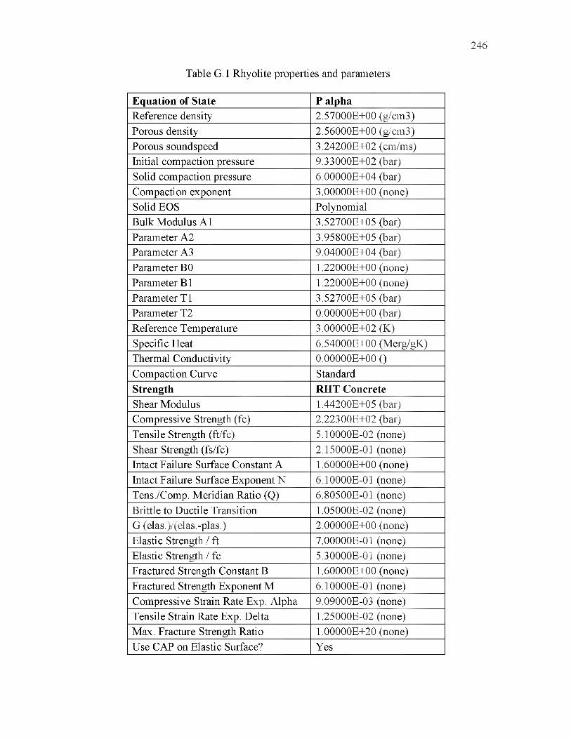
246

Table G.1 Rhyolite properties and parameters

Equation of State P alphaReference density 2.57000E+00 (g/cm3)Porous density 2.56000E+00 (g/cm3)Porous soundspeed 3.24200E+02 (cm/ms)Initial compaction pressure 9.33000E+02 (bar)Solid compaction pressure 6.00000E+04 (bar)Compaction exponent 3.00000E+00 (none)Solid EOS PolynomialBulk Modulus A1 3.52700E+05 (bar)Parameter A2 3.95800E+05 (bar)Parameter A3 9.04000E+04 (bar)Parameter B0 1.22000E+00 (none)Parameter B 1 1.22000E+00 (none)Parameter T1 3.52700E+05 (bar)Parameter T2 0.00000E+00 (bar)Reference Temperature 3.00000E+02 (K)Specific Heat 6.54000E+00 (Merg/gK)Thermal Conductivity 0.00000E+00 ()Compaction Curve StandardStrength RHT ConcreteShear Modulus 1.44200E+05 (bar)Compressive Strength (fc) 2.22300E+02 (bar)Tensile Strength (ft/fc) 5.10000E-02 (none)Shear Strength (fs/fc) 2.15000E-01 (none)Intact Failure Surface Constant A 1.60000E+00 (none)Intact Failure Surface Exponent N 6.10000E-01 (none)Tens./Comp. Meridian Ratio (Q) 6.80500E-01 (none)Brittle to Ductile Transition 1.05000E-02 (none)G (elas.)/(elas.-plas.) 2.00000E+00 (none)Elastic Strength / ft 7.00000E-01 (none)Elastic Strength / fc 5.30000E-01 (none)Fractured Strength Constant B 1.60000E+00 (none)Fractured Strength Exponent M 6.10000E-01 (none)Compressive Strain Rate Exp. Alpha 9.09000E-03 (none)Tensile Strain Rate Exp. Delta 1.25000E-02 (none)Max. Fracture Strength Ratio 1.00000E+20 (none)Use CAP on Elastic Surface? Yes

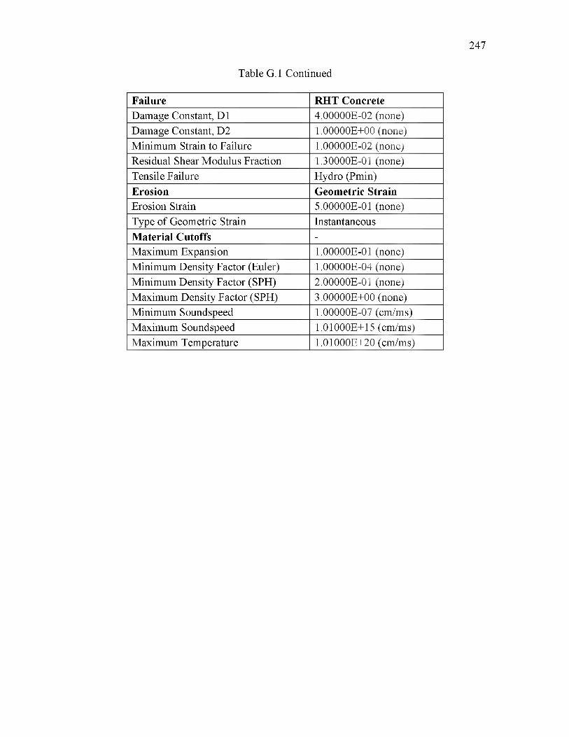
247

Table G.1 Continued

Failure RHT ConcreteDamage Constant, D1 4.00000E-02 (none)Damage Constant, D2 1.00000E+00 (none)Minimum Strain to Failure 1.00000E-02 (none)Residual Shear Modulus Fraction 1.30000E-01 (none)Tensile Failure Hydro (Pmin)Erosion Geometric StrainErosion Strain 5.00000E-01 (none)Type of Geometric Strain InstantaneousMaterial Cutoffs -Maximum Expansion 1.00000E-01 (none)Minimum Density Factor (Euler) 1.00000E-04 (none)Minimum Density Factor (SPH) 2.00000E-01 (none)Maximum Density Factor (SPH) 3.00000E+00 (none)Minimum Soundspeed 1.00000E-07 (cm/ms)Maximum Soundspeed 1.01000E+15 (cm/ms)Maximum Temperature 1.01000E+20 (cm/ms)

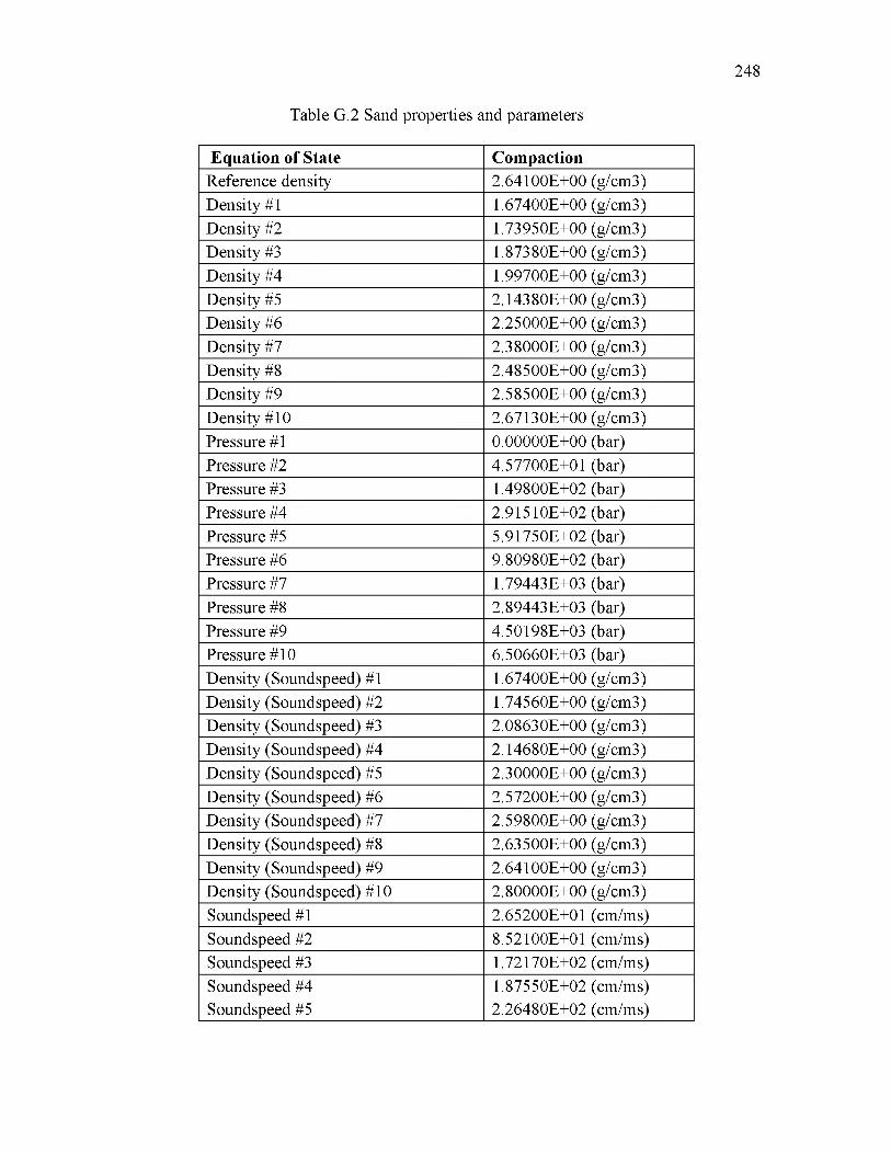
248

Table G.2 Sand properties and parameters

Equation of State CompactionReference density 2.64100E+00 (g/cm3)Density #1 1.67400E+00 (g/cm3)Density #2 1.73950E+00 (g/cm3)Density #3 1.87380E+00 (g/cm3)Density #4 1.99700E+00 (g/cm3)Density #5 2.14380E+00 (g/cm3)Density #6 2.25000E+00 (g/cm3)Density #7 2.38000E+00 (g/cm3)Density #8 2.48500E+00 (g/cm3)Density #9 2.58500E+00 (g/cm3)Density #10 2.67130E+00 (g/cm3)Pressure #1 0.00000E+00 (bar)Pressure #2 4.57700E+01 (bar)Pressure #3 1.49800E+02 (bar)Pressure #4 2.91510E+02 (bar)Pressure #5 5.91750E+02 (bar)Pressure #6 9.80980E+02 (bar)Pressure #7 1.79443E+03 (bar)Pressure #8 2.89443E+03 (bar)Pressure #9 4.50198E+03 (bar)Pressure #10 6.50660E+03 (bar)Density (Soundspeed) #1 1.67400E+00 (g/cm3)Density (Soundspeed) #2 1.74560E+00 (g/cm3)Density (Soundspeed) #3 2.08630E+00 (g/cm3)Density (Soundspeed) #4 2.14680E+00 (g/cm3)Density (Soundspeed) #5 2.30000E+00 (g/cm3)Density (Soundspeed) #6 2.57200E+00 (g/cm3)Density (Soundspeed) #7 2.59800E+00 (g/cm3)Density (Soundspeed) #8 2.63500E+00 (g/cm3)Density (Soundspeed) #9 2.64100E+00 (g/cm3)Density (Soundspeed) #10 2.80000E+00 (g/cm3)Soundspeed #1 2.65200E+01 (cm/ms)Soundspeed #2 8.52100E+01 (cm/ms)Soundspeed #3 1.72170E+02 (cm/ms)Soundspeed #4 1.87550E+02 (cm/ms)Soundspeed #5 2.26480E+02 (cm/ms)

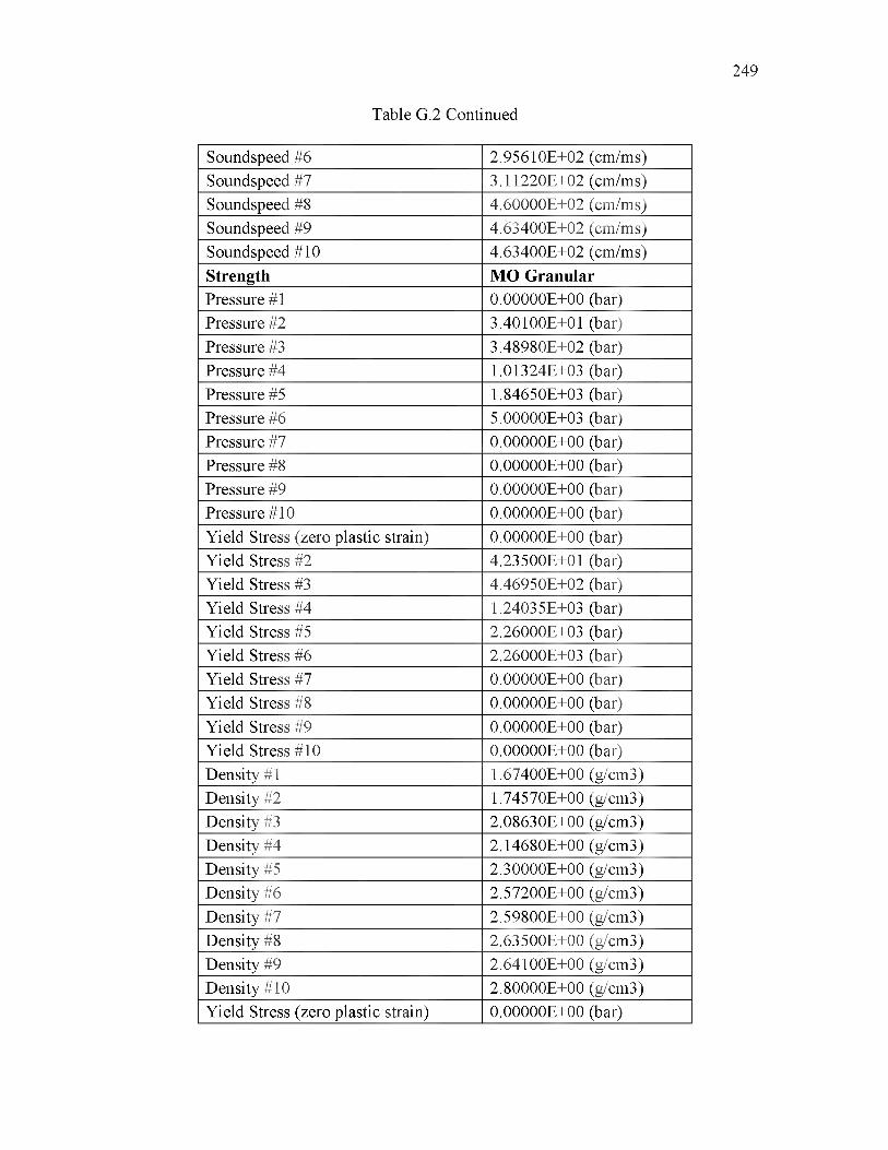
249

Table G.2 Continued

Soundspeed #6 2.95610E+02 (cm/ms)Soundspeed #7 3.11220E+02 (cm/ms)Soundspeed #8 4.60000E+02 (cm/ms)Soundspeed #9 4.63400E+02 (cm/ms)Soundspeed #10 4.63400E+02 (cm/ms)Strength MO GranularPressure #1 0.00000E+00 (bar)Pressure #2 3.40100E+01 (bar)Pressure #3 3.48980E+02 (bar)Pressure #4 1.01324E+03 (bar)Pressure #5 1.84650E+03 (bar)Pressure #6 5.00000E+03 (bar)Pressure #7 0.00000E+00 (bar)Pressure #8 0.00000E+00 (bar)Pressure #9 0.00000E+00 (bar)Pressure #10 0.00000E+00 (bar)Yield Stress (zero plastic strain) 0.00000E+00 (bar)Yield Stress #2 4.23500E+01 (bar)Yield Stress #3 4.46950E+02 (bar)Yield Stress #4 1.24035E+03 (bar)Yield Stress #5 2.26000E+03 (bar)Yield Stress #6 2.26000E+03 (bar)Yield Stress #7 0.00000E+00 (bar)Yield Stress #8 0.00000E+00 (bar)Yield Stress #9 0.00000E+00 (bar)Yield Stress #10 0.00000E+00 (bar)Density #1 1.67400E+00 (g/cm3)Density #2 1.74570E+00 (g/cm3)Density #3 2.08630E+00 (g/cm3)Density #4 2.14680E+00 (g/cm3)Density #5 2.30000E+00 (g/cm3)Density #6 2.57200E+00 (g/cm3)Density #7 2.59800E+00 (g/cm3)Density #8 2.63500E+00 (g/cm3)Density #9 2.64100E+00 (g/cm3)Density #10 2.80000E+00 (g/cm3)Yield Stress (zero plastic strain) 0.00000E+00 (bar)

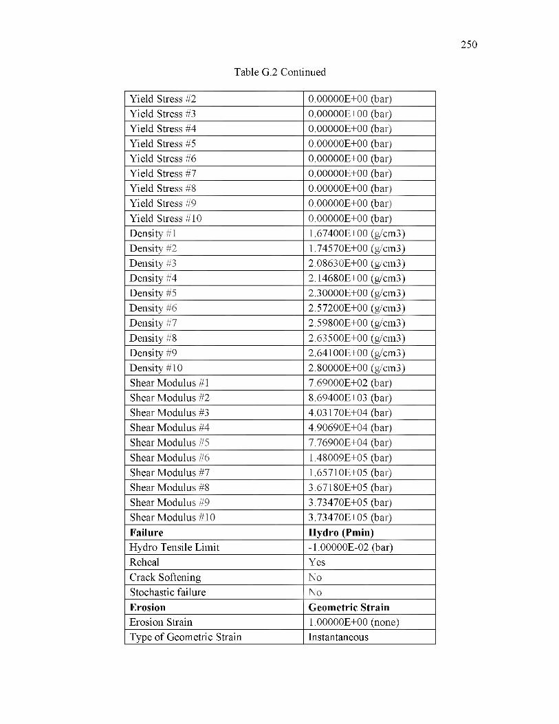
250

Table G.2 Continued

Yield Stress #2 0.00000E+00 (bar)Yield Stress #3 0.00000E+00 (bar)Yield Stress #4 0.00000E+00 (bar)Yield Stress #5 0.00000E+00 (bar)Yield Stress #6 0.00000E+00 (bar)Yield Stress #7 0.00000E+00 (bar)Yield Stress #8 0.00000E+00 (bar)Yield Stress #9 0.00000E+00 (bar)Yield Stress #10 0.00000E+00 (bar)Density #1 1.67400E+00 (g/cm3)Density #2 1.74570E+00 (g/cm3)Density #3 2.08630E+00 (g/cm3)Density #4 2.14680E+00 (g/cm3)Density #5 2.30000E+00 (g/cm3)Density #6 2.57200E+00 (g/cm3)Density #7 2.59800E+00 (g/cm3)Density #8 2.63500E+00 (g/cm3)Density #9 2.64100E+00 (g/cm3)Density #10 2.80000E+00 (g/cm3)Shear Modulus #1 7.69000E+02 (bar)Shear Modulus #2 8.69400E+03 (bar)Shear Modulus #3 4.03170E+04 (bar)Shear Modulus #4 4.90690E+04 (bar)Shear Modulus #5 7.76900E+04 (bar)Shear Modulus #6 1.48009E+05 (bar)Shear Modulus #7 1.65710E+05 (bar)Shear Modulus #8 3.67180E+05 (bar)Shear Modulus #9 3.73470E+05 (bar)Shear Modulus #10 3.73470E+05 (bar)Failure Hydro (Pmin)Hydro Tensile Limit -1.00000E-02 (bar)Reheal YesCrack Softening NoStochastic failure NoErosion Geometric StrainErosion Strain 1.00000E+00 (none)Type of Geometric Strain Instantaneous

251

Table G.2 Continued

Material Cutoffs -Maximum Expansion 1.00000E-01 (none)Minimum Density Factor (Euler) 1.00000E-04 (none)Minimum Density Factor (SPH) 2.00000E-01 (none)Maximum Density Factor (SPH) 3.00000E+00 (none)Minimum Soundspeed 1.00000E-07 (cm/ms)Maximum Soundspeed 1.01000E+15 (cm/ms)Maximum Temperature 1.01000E+20 (cm/ms)

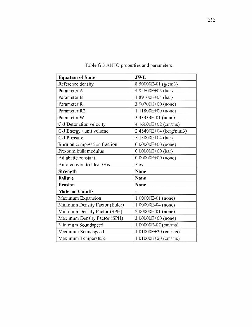
252

Table G.3 ANFO properties and parameters

Equation of State JWLReference density 8.50000E-01 (g/cm3)Parameter A 4.94600E+05 (bar)Parameter B 1.89100E+04 (bar)Parameter R1 3.90700E+00 (none)Parameter R2 1.11800E+00 (none)Parameter W 3.33333E-01 (none)C-J Detonation velocity 4.16000E+02 (cm/ms)C-J Energy / unit volume 2.48400E+04 (kerg/mm3)C-J Pressure 5.15000E+04 (bar)Burn on compression fraction 0.00000E+00 (none)Pre-burn bulk modulus 0.00000E+00 (bar)Adiabatic constant 0.00000E+00 (none)Auto-convert to Ideal Gas YesStrength NoneFailure NoneErosion NoneMaterial Cutoffs -Maximum Expansion 1.00000E-01 (none)Minimum Density Factor (Euler) 1.00000E-04 (none)Minimum Density Factor (SPH) 2.00000E-01 (none)Maximum Density Factor (SPH) 3.00000E+00 (none)Minimum Soundspeed 1.00000E-07 (cm/ms)Maximum Soundspeed 1.01000E+20 (cm/ms)Maximum Temperature 1.01000E+20 (cm/ms)

253

Table G.4 Air properties and parameters

Equation of State Ideal GasReference density 1.22500E-03 (g/cm3)Gamma 1.40000E+00 (none)Adiabatic constant 0.00000E+00 (none)Pressure shift 0.00000E+00 (bar)Reference Temperature 2.88200E+02 (K)Specific Heat 7.17600E+00 (Merg/gK)Thermal Conductivity 0.00000E+00 ()Strength NoneFailure NoneErosion NoneMaterial Cutoffs -Maximum Expansion 1.00000E-01 (none)Minimum Density Factor (Euler) 1.00000E-04 (none)Minimum Density Factor (SPH) 2.00000E-01 (none)Maximum Density Factor (SPH) 3.00000E+00 (none)Minimum Soundspeed 1.00000E-03 (cm/ms)Maximum Soundspeed 1.01000E+15 (cm/ms)Maximum Temperature 1.01000E+20 (cm/ms)

APPENDIX H

PYTHON CODE FOR LEAST SQUARES

VIBRATION MODEL

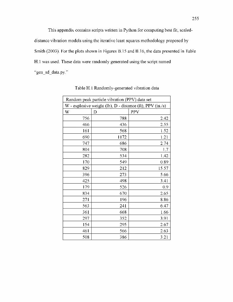
This appendix contains scripts written in Python for computing best fit, scaled-

distance vibration models using the iterative least squares methodology proposed by

Smith (2003). For the plots shown in Figures B.15 and B.16, the data presented in Table

H.1 was used. These data were randomly generated using the script named

“gen_sd_data.py.”

255

Table H.1 Randomly-generated vibration data

Random peak particle vibration (PPV) data setW - explosive weight (lb), D - distance (ft), PPV (in./s)W D PPV

756 788 2.42466 436 2.55161 568 1.52690 1172 1.21747 686 2.74804 708 1.7282 534 1.42170 549 0.89829 212 15.57396 273 5.66425 498 3.41179 526 0.9834 670 2.65271 196 8.86563 241 6.47361 668 1.66297 352 3.91154 295 2.67461 566 2.63508 386 3.21

256

H.1 Python script for randomly generating vibration data

gen_sd_data.py

Author: Kirk Erickson

Program to randomly generate scaled distance data for blast vibration analysis. Based on the empirical equation PPV = k(SD)A-B, where SD = R/WA(a/B).i iiii i

''' To run code, first set working directory using os.chdir() command, then execute file using execfile() command.'''# os.chdir('C:\Users\Kirk\U of U\M.S. thesis\LSM vibration model')# execfile(‘gen_sd_data.py')

# Import modules import numpy as np

# Input parameters'''Note: Program originally written for units of lb, ft, and ips''' sc_law = 0.4 # Scaling lawB = 1.6 a = B*sc_law k = 700.W_range = np.array([100.,900.]) # Range of charge weights SD_range = np.array([10.,90.]) # Range of scaled distance values N = 20 # size of data setfactor = 1.2 # Amount by which data can randomly vary

# Generate random dataSD = np.random.random(N)*(SD_range[1]-SD_range[0])+SD_range[0]# Generate scaled distancesW = np.random.random(N)*(W_range[1]-W_range[0])+W_range[0]# Generate charge weightsR = np.multiply(SD,np.power(W,sc_law)) # Calulate distances PPV = np.multiply(k,np.power(SD,-B)) # Calculate PPV values PPV += np.multiply(np.random.random(N),PPV)*factor # Randomize PPV data

# Write values to filesavedir = 'C:\Users\Kirk\U of U\M.S. thesis\LSM vibration model\\' filename = savedir + 'rnd_data.txt' # File name to write data to fid = open(filename,'w')fid.write('Random peak particle vibration (PPV) data set\n') fid.write('W - explosive weight (lb), D - distance (ft), PPV (ips)\n') fid.write('W\tD\tPPV\n')

for i in np.arange(N): fid.write('{0:5.0f}\t{1:5.0f}\t{2:5.2f}\n'.format(W[i],R[i],PPV[i]))

fid.close()

257

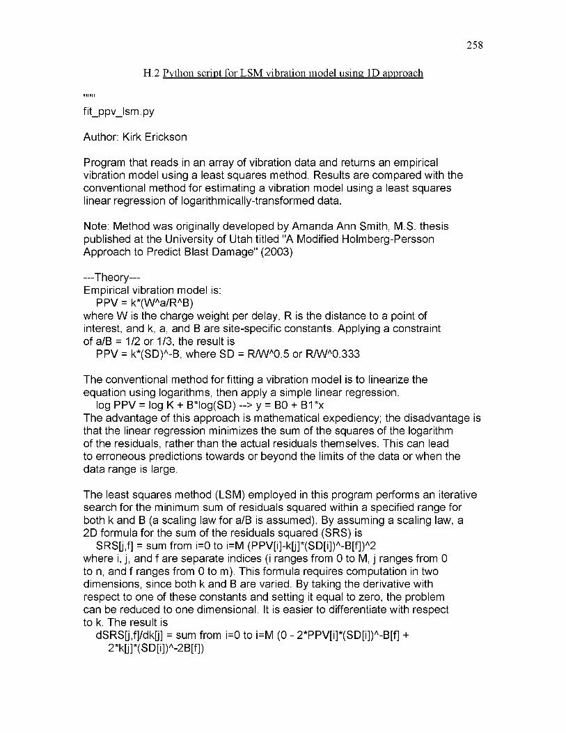
258

IIIIII

fit_ppv_lsm.py

Author: Kirk Erickson

Program that reads in an array of vibration data and returns an empirical vibration model using a least squares method. Results are compared with the conventional method for estimating a vibration model using a least squares linear regression of logarithmically-transformed data.

Note: Method was originally developed by Amanda Ann Smith, M.S. thesis published at the University of Utah titled "A Modified Holmberg-Persson Approach to Predict Blast Damage" (2003)

---Theory---Empirical vibration model is:

PPV = k*(WAa/RAB) where W is the charge weight per delay, R is the distance to a point of interest, and k, a, and B are site-specific constants. Applying a constraint of a/B = 1/2 or 1/3, the result is

PPV = k*(SD)A-B, where SD = R/WA0.5 or R W 0 .3 3 3

The conventional method for fitting a vibration model is to linearize the equation using logarithms, then apply a simple linear regression.

log PPV = log K + B*log(SD) --> y = B0 + B1*x The advantage of this approach is mathematical expediency; the disadvantage is that the linear regression minimizes the sum of the squares of the logarithm of the residuals, rather than the actual residuals themselves. This can lead to erroneous predictions towards or beyond the limits of the data or when the data range is large.

The least squares method (LSM) employed in this program performs an iterative search for the minimum sum of residuals squared within a specified range for both k and B (a scaling law for a/B is assumed). By assuming a scaling law, a 2D formula for the sum of the residuals squared (SRS) is

SRS[j,f] = sum from i=0 to i=M (PPV[i]-k[j]*(SD[i])A-B[f])A2 where i, j, and f are separate indices (i ranges from 0 to M, j ranges from 0 to n, and f ranges from 0 to m). This formula requires computation in two dimensions, since both k and B are varied. By taking the derivative with respect to one of these constants and setting it equal to zero, the problem can be reduced to one dimensional. It is easier to differentiate with respect to k. The result is

dSRS[j,f]/dk[j] = sum from i=0 to i=M (0 - 2*PPV[i]*(SD[i])A-B[f] + 2*k[j]*(SD[i])A-2B[f])

H.2 Python script for LSM vibration model using 1D approach

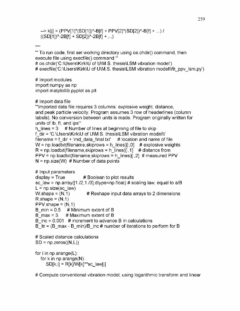
259

--> k[j] = (PPV[1]*(SD[1])A-B[f] + PPV[2]*(SD[2])A-B[f] + ...) /((SD[1])A-2B[f] + SD[2])A-2B[f] + ...)

i ii ii i

''' To run code, first set working directory using os.chdir() command, then execute file using execfile() command.'''# os.chdir('C:\Users\Kirk\U of U\M.S. thesis\LSM vibration model')# execfile('C:\Users\Kirk\U of U\M.S. thesis\LSM vibration model\\fit_ppv_lsm.py')

# Import modules import numpy as npimport matplotlib.pyplot as plt

# Import data file'''Imported data file requires 3 columns: explosive weight, distance, and peak particle velocity. Program assumes 3 row of headerlines (column labels). No conversion between units is made. Program originally written for units of lb, ft, and ips'''h_lines = 3 # Number of lines at beginning of file to skip f_dir = 'C:\Users\Kirk\U of U\M.S. thesis\LSM vibration model\\' filename = f_dir + 'rnd_data_final.txt' # location and name of file W = np.loadtxt(filename,skiprows = h_lines)[:,0] # explosive weights R = np.loadtxt(filename,skiprows = h_lines)[:,1] # distance from PPV = np.loadtxt(filename,skiprows = h_lines)[:,2] # measured PPV N = np.size(W) # Number of data points

# Input parametersdisplay = True # Boolean to plot resultssc_law = np.array([1 ./2,1./3],dtype=np.float) # scaling law; equal to a/BL = np.size(sc_law)W.shape = (N,1) # Reshape input data arrays to 2 dimensionsR.shape = (N,1)PPV.shape = (N,1)B_min = 0.5 # Minimum extent of BB_max = 3. # Maximum extent of BB_inc = 0.001 # increment to advance B in calculationsB_itr = (B_max - B_min)/B_inc # number of iterations to perform for B

# Scaled distance calculations SD = np.zeros((N,L))

for i in np.arange(L): for k in np.arange(N):

SD[k,i] = R[k]/W[k]**sc_law[i]

# Compute conventional vibration model, using logarithmic transform and linear

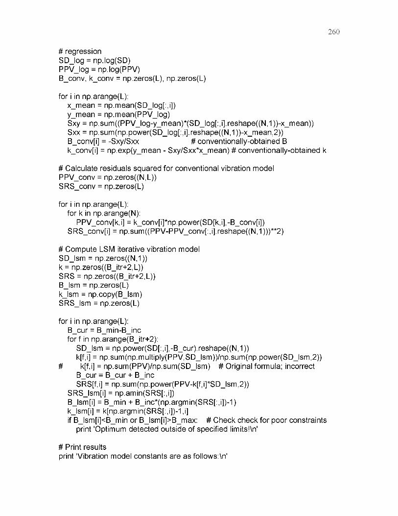
# regression SD_log = np.log(SD)PPV_log = np.log(PPV)B_conv, k_conv = np.zeros(L), np.zeros(L)

for i in np.arange(L):x_mean = np.mean(SD_log[:,i]) y_mean = np.mean(PPV_log)Sxy = np.sum((PPV_log-y_mean)*(SD_log[:,i].reshape((N,1))-x_mean))Sxx = np.sum(np.power(SD_log[:,i].reshape((N,1))-x_mean,2))B_conv[i] = -Sxy/Sxx # conventionally-obtained Bk_conv[i] = np.exp(y_mean - Sxy/Sxx*x_mean) # conventionally-obtained k

# Calculate residuals squared for conventional vibration model PPV_conv = np.zeros((N,L))SRS_conv = np.zeros(L)

for i in np.arange(L): for k in np.arange(N):

PPV_conv[k,i] = k_conv[i]*np.power(SD[k,i],-B_conv[i])SRS_conv[i] = np.sum((PPV-PPV_conv[:,i].reshape((N,1)))**2)

# Compute LSM iterative vibration model SD_lsm = np.zeros((N,1))k = np.zeros((B_itr+2,L))SRS = np.zeros((B_itr+2,L))B_lsm = np.zeros(L) k_lsm = np.copy(B_lsm)SRS_lsm = np.zeros(L)

for i in np.arange(L):B_cur = B_min-B_inc for f in np.arange(B_itr+2):

SD_lsm = np.power(SD[:,i],-B_cur).reshape((N,1))k[f,i] = np.sum(np.multiply(PPV,SD_lsm))/np.sum(np.power(SD_lsm,2))

# k[f,i] = np.sum(PPV)/np.sum(SD_lsm) # Original formula; incorrect B_cur = B_cur + B_incSRS[f,i] = np.sum(np.power(PPV-k[f,i]*SD_lsm,2))

SRS_lsm[i] = np.amin(SRS[:,i])B_lsm[i] = B_min + B_inc*(np.argmin(SRS[:,i])-1) k_lsm[i] = k[np.argmin(SRS[:,i])-1,i]if B_lsm[i]<B_min or B_lsm[i]>B_max: # Check check for poor constraints

print 'Optimum detected outside of specified limits!\n'

# Print resultsprint 'Vibration model constants are as follows:\n'

260

261

for i in range(L):print 'Scaling law a/B = {:5.3f}'.format(sc_law[i]) print 'Value \tLog \tLSM \t'print 'B \t{0:>8.3f}\t{1:>8.3f}'.format(B_conv[i],B_lsm[i]) print 'k \t{0:>7.2f}\t{1 :>7.2f}'.format(k_conv[i],k_lsm[i]) print 'SRS \t{0:>8.3f}\t{1:>8.3f}\format(SRS_conv[i],sRs_lsm[i]) print '\n'

del(Sxy,Sxx,x_mean,y_mean,SD_log,PPV_log)del(B_cur,B_min)

# Display results if display:

plt.close()

if L>16: # No plot generated if more than 16 figures to be plotted print 'Number of subplots exceeds maximum of 16!'

else:s1 = np.int(np.ceil(np.sqrt(L))) # Determine arrangement of subplots s2 = np.int(L-s1) if s2==0:

s2 = 1 elif s2*s1<L:

s2 += 1s_cur = 1 # Current subplot number

for i in np.arange(L):plt.subplot(s1 ,s2,s_cur) # Subplot numberxaxis = np.linspace(np.amin(SD[:,i]),np.amax(SD[:,i]))yaxis1 = k_conv[i]*np.power(xaxis,-B_conv[i])yaxis2 = k_lsm[i]*np.power(xaxis,-B_lsm[i])plt.plot(SD[:,i],PPV,'rs',xaxis,yaxis1,'--k',xaxis,yaxis2,'-k')if s_cur==1:

plt.suptitle('Comparison of vibration models',fontsize=18)# sc_show = '{0:0.3f}'.format(sc_law[i]) # For showing superscript# plt.xlabel('Scaled distance 'r'$R/WA{+sc_show+'}$')

plt.xlabel('Scaled distance 'r'$R/W$A${0:5.3f}$'.format(sc_law[i])) plt.ylabel('PPV, 'r'$\alpha/\beta={0:5.3f}$'.format(sc_law[i])) plt.legend(('Data','Log','LSM'))s_cur = s_cur + 1

mng = plt.get_current_fig_manager() mng.window.showMaximized() # Maximize figure window plt.show()

262

del(s1 ,s2,s_cur,xaxis,yaxis1,yaxis2) del(display,SD_lsm)

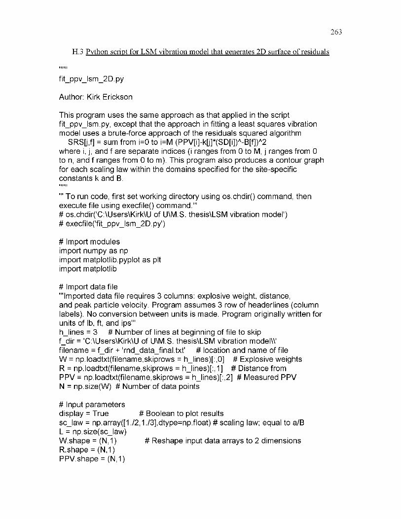
263

IIIIII

fit_ppv_lsm_2D.py

Author: Kirk Erickson

This program uses the same approach as that applied in the scriptfit_ppv_lsm.py, except that the approach in fitting a least squares vibrationmodel uses a brute-force approach of the residuals squared algorithm

SRS[j,f] = sum from i=0 to i=M (PPV[i]-k[j]*(SD[i])A-B[f])A2where i, j, and f are separate indices (i ranges from 0 to M, j ranges from 0to n, and f ranges from 0 to m). This program also produces a contour graphfor each scaling law within the domains specified for the site-specificconstants k and B. i ii ii i

''' To run code, first set working directory using os.chdir() command, then execute file using execfile() command.'''# os.chdir('C:\Users\Kirk\U of U\M.S. thesis\LSM vibration model')# execfile('fit_ppv_lsm_2D.py')

# Import modules import numpy as npimport matplotlib.pyplot as plt import matplotlib

# Import data file'''Imported data file requires 3 columns: explosive weight, distance, and peak particle velocity. Program assumes 3 row of headerlines (column labels). No conversion between units is made. Program originally written for units of lb, ft, and ips'''h_lines = 3 # Number of lines at beginning of file to skip f_dir = 'C:\Users\Kirk\U of U\M.S. thesis\LSM vibration model\\' filename = f_dir + 'rnd_data_final.txt' # location and name of file W = np.loadtxt(filename,skiprows = h_lines)[:,0] # Explosive weights R = np.loadtxt(filename,skiprows = h_lines)[:,1] # Distance from PPV = np.loadtxt(filename,skiprows = h_lines)[:,2] # Measured PPV N = np.size(W) # Number of data points

# Input parametersdisplay = True # Boolean to plot resultssc_law = np.array([1 ./2,1./3],dtype=np.float) # scaling law; equal to a/BL = np.size(sc_law)W.shape = (N,1) # Reshape input data arrays to 2 dimensionsR.shape = (N,1)PPV.shape = (N,1)

H.3 Python script for LSM vibration model that generates 2D surface of residuals

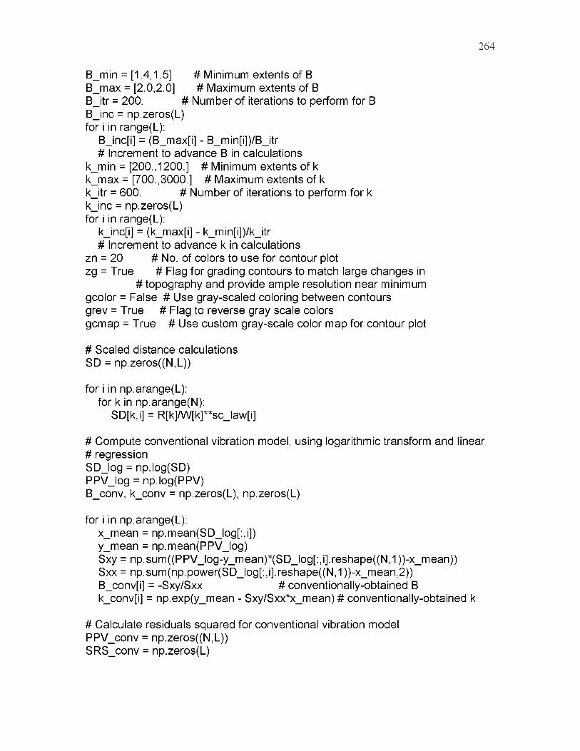
264

B_min = [1.4,1.5] # Minimum extents of BB_max = [2.0,2.0] # Maximum extents of BB_itr = 200. # Number of iterations to perform for BB_inc = np.zeros(L)for i in range(L):

B_inc[i] = (B_max[i] - B_min[i])/B_itr# Increment to advance B in calculations

k_min = [200.,1200.] # Minimum extents of k k_max = [700.,3000.] # Maximum extents of kk_itr = 600. # Number of iterations to perform for kk_inc = np.zeros(L) for i in range(L):

k_inc[i] = (k_max[i] - k_min[i])/k_itr# Increment to advance k in calculations

zn = 20 # No. of colors to use for contour plot zg = True # Flag for grading contours to match large changes in

# topography and provide ample resolution near minimum gcolor = False # Use gray-scaled coloring between contours grev = True # Flag to reverse gray scale colors gcmap = True # Use custom gray-scale color map for contour plot

# Scaled distance calculations SD = np.zeros((N,L))

for i in np.arange(L): for k in np.arange(N):

SD[k,i] = R[k]/W[k]**sc_law[i]

# Compute conventional vibration model, using logarithmic transform and linear# regression SD_log = np.log(SD)PPV_log = np.log(PPV)B_conv, k_conv = np.zeros(L), np.zeros(L)

for i in np.arange(L):x_mean = np.mean(SD_log[:,i]) y_mean = np.mean(PPV_log)Sxy = np.sum((PPV_log-y_mean)*(SD_log[:,i].reshape((N,1))-x_mean))Sxx = np.sum(np.power(SD_log[:,i].reshape((N,1))-x_mean,2))B_conv[i] = -Sxy/Sxx # conventionally-obtained Bk_conv[i] = np.exp(y_mean - Sxy/Sxx*x_mean) # conventionally-obtained k

# Calculate residuals squared for conventional vibration model PPV_conv = np.zeros((N,L))SRS_conv = np.zeros(L)

265

for i in np.arange(L): for k in np.arange(N):

PPV_conv[k,i] = k_conv[i]*np.power(SD[k,i],-B_conv[i])SRS_conv[i] = np.sum((PPV-PPV_conv[:,i].reshape((N,1)))**2)

# Compute LSM iterative vibration model SD_lsm = np.zeros((N,1))SRS = np.zeros((L,B_itr+2,k_itr+2))B_lsm = np.zeros(L) k_lsm = np.copy(B_lsm)SRS_lsm = np.zeros(L)SRS_max = np.copy(SRS_lsm)

for i in np.arange(L):B_cur = B_min[i]-B_inc[i] for f in np.arange(B_itr+2):

SD_lsm = np.power(SD[:,i],-B_cur).reshape((N,1)) k_cur = k_min[i] - k_inc[i] for j in np.arange(k_itr+2):

SRS[i,f,j] = np.sum(np.power(PPV-k_cur*SD_lsm,2)) k_cur += k_inc[i]

B_cur += B_inc[i]SRS_lsm[i] = np.amin(SRS[i,1: B_itr+1,1 :k_itr+1 ])SRS_max[i] = np.amax(SRS[i,1:B_itr+1,1:k_itr+1]) mindex = np.unravel_index(np.argmin(SRS[i,:,:]),(B_itr+2,k_itr+2)) B_lsm[i] = B_min[i] + B_inc[i]*(mindex[0]-1) k_lsm[i] = k_min[i] + k_inc[i]*(mindex[1]-1) if B_lsm[i]<B_min[i] or B_lsm[i]>B_max[i] or k_lsm[i]<k_min[i] or \

k_lsm[i]>k_max[i]: # Check check for poor constraints print 'Optimum detected outside of specified limits!'

# Print resultsprint '\nVibration model constants are as follows:\n' for i in range(L):

print 'Scaling law a/B = {:5.3f}'.format(sc_law[i]) print 'Value \tLog \tLSM \t'print 'B \t{0:>8.3f}\t{1 :>8.3f}'.format(B_conv[i],B_lsm[i]) print 'k \t{0:>7.2f}\t{1 :>7.2f}'.format(k_conv[i],k_lsm[i]) print 'SRS \t{0:>8.3f}\t{1:>8.3f}'.format(SRS_conv[i],SRS_lsm[i]) print '\n'

del(Sxy,Sxx,x_mean,y_mean,SD_log,PPV_log)del(B_cur,k_cur)

# Custom grayscale colormap for plotting exponentially-increasing contour# levels

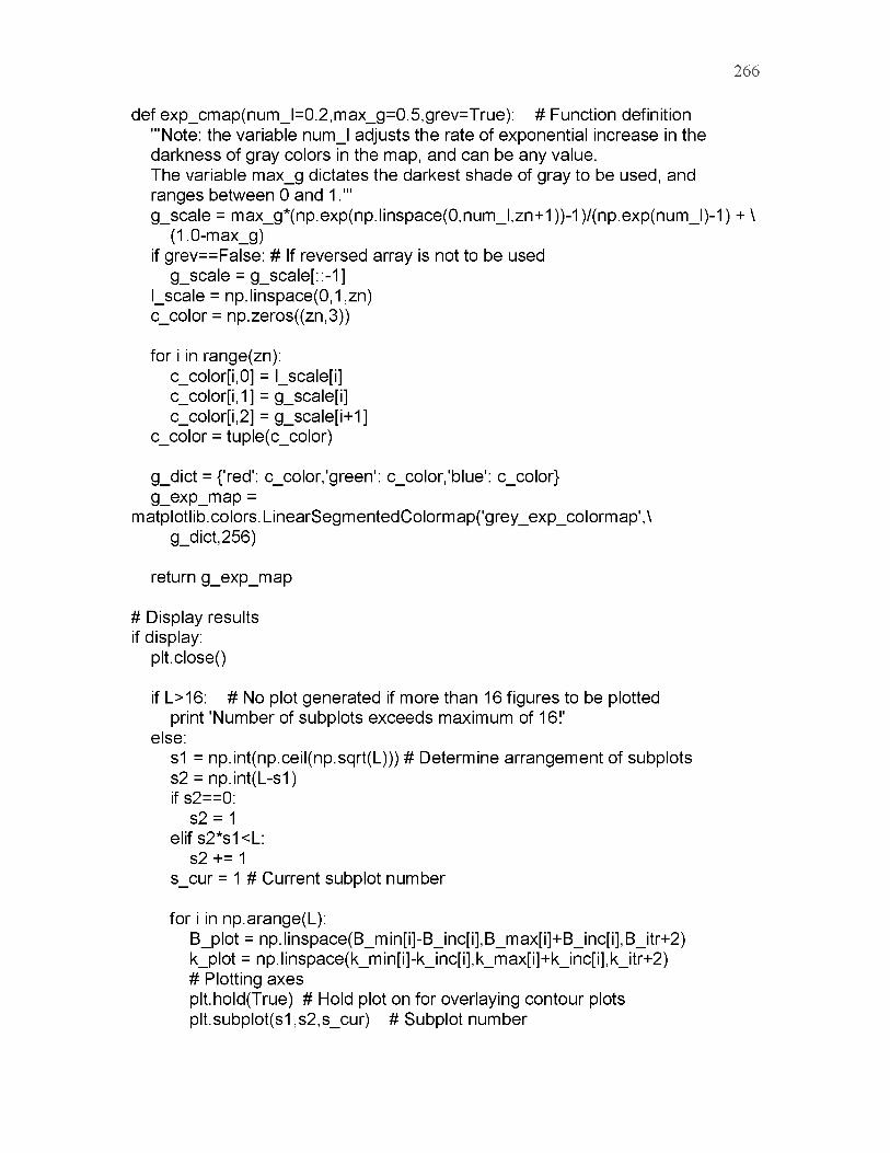
266

def exp_cmap(num_l=0.2,max_g=0.5,grev=True): # Function definition '''Note: the variable num_l adjusts the rate of exponential increase in the darkness of gray colors in the map, and can be any value.The variable max_g dictates the darkest shade of gray to be used, and ranges between 0 and 1.'''g_scale = max_g*(np.exp(np.linspace(0,num_l,zn+1))-1)/(np.exp(num_l)-1) + \

(1.0-max_g)if grev==False: # If reversed array is not to be used

g_scale = g_scale[::-1] l_scale = np.linspace(0,1,zn) c_color = np.zeros((zn,3))

for i in range(zn):c_color[i,0] = l_scale[i] c_color[i,1] = g_scale[i] c_color[i,2] = g_scale[i+1]

c_color = tuple(c_color)

g_dict = {'red': c_color,'green': c_color,'blue': c_color} g_exp_map =

matplotlib.colors.LinearSegmentedColormap('grey_exp_colormap',\g_dict,256)

return g_exp_map

# Display results if display:

plt.close()

if L>16: # No plot generated if more than 16 figures to be plotted print 'Number of subplots exceeds maximum of 16!'

else:s1 = np.int(np.ceil(np.sqrt(L))) # Determine arrangement of subplots s2 = np.int(L-s1) if s2==0:

s2 = 1 elif s2*s1<L:

s2 += 1s_cur = 1 # Current subplot number

for i in np.arange(L):B_plot = np.linspace(B_min[i]-B_inc[i],B_max[i]+B_inc[i],B_itr+2) k_plot = np.linspace(k_min[i]-k_inc[i],k_max[i]+k_inc[i],k_itr+2)# Plotting axesplt.hold(True) # Hold plot on for overlaying contour plots plt.subplot(s1 ,s2,s_cur) # Subplot number

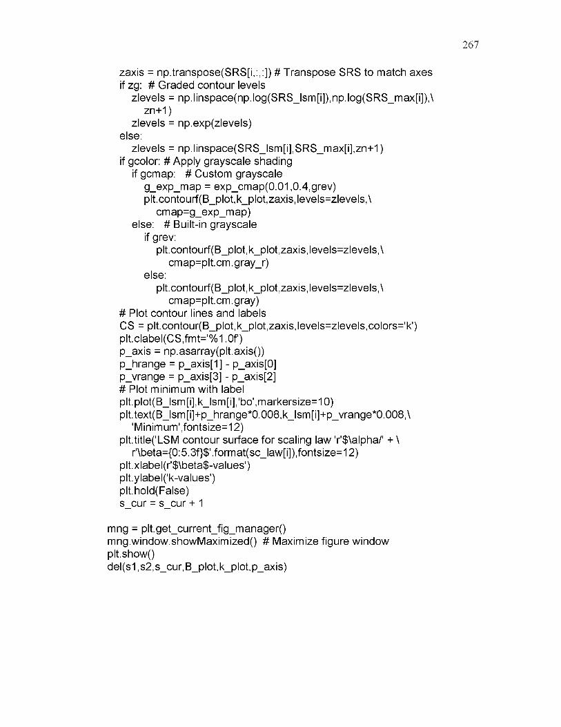
267

zaxis = np.transpose(SRS[i,:,:]) # Transpose SRS to match axes if zg: # Graded contour levels

zlevels = np.linspace(np.log(SRS_lsm[i]),np.log(SRS_max[i]),\ zn+1)

zlevels = np.exp(zlevels) else:

zlevels = np.linspace(SRS_lsm[i],SRS_max[i],zn+1) if gcolor: # Apply grayscale shading

if gcmap: # Custom grayscale g_exp_map = exp_cmap(0.01,0.4,grev) plt.contourf(B_plot,k_plot,zaxis,levels=zlevels,\

cmap=g_exp_map) else: # Built-in grayscale

if grev:plt.contourf(B_plot,k_plot,zaxis,levels=zlevels,\

cmap=plt.cm.gray_r)else:

plt.contourf(B_plot,k_plot,zaxis,levels=zlevels,\cmap=plt.cm.gray)

# Plot contour lines and labelsCS = plt.contour(B_plot,k_plot,zaxis,levels=zlevels,colors='k')plt.clabel(CS,fmt='%1.0f')p_axis = np.asarray(plt.axis())p_hrange = p_axis[1] - p_axis[0]p_vrange = p_axis[3] - p_axis[2]# Plot minimum with label plt.plot(B_lsm[i],k_lsm[i],'bo',markersize=10) plt.text(B_lsm[i]+p_hrange*0.008,k_lsm[i]+p_vrange*0.008,\

'Minimum',fontsize=12) plt.title('LSM contour surface for scaling law 'r'$\alpha/' + \

r'\beta={0:5.3f}$'.format(sc_law[i]),fontsize=12) plt.xlabel(r'$\beta$-values') plt.ylabel('k-values') plt.hold(False) s_cur = s_cur + 1

mng = plt.get_current_fig_manager() mng.window.showMaximized() # Maximize figure window plt.show()del(s1,s2,s_cur,B_plot,k_plot,p_axis)

APPENDIX I

THE FAST FOURIER TRANSFORM

During the course of the author’s studies, a considerable amount of time and

effort was spent on learning and applying the basics of digital signal analysis with the

Fourier transform to apply in research for this thesis. It is only reasonable that at least an

overview of the knowledge acquired should be passed on for other individuals to use. For

those who are unfamiliar with digital signal processing and wish to expand their

knowledge beyond the contents of this appendix, Fundamentals o f Signals and Systems

by Cha and Molinder (2006) is highly recommended for both its accessibility and brevity.

In this appendix, a basic overview of the Fast Fourier Transform (FFT) is

presented. Python code is attached for calculating and plotting a frequency spectrum from

an input vibration waveform.

I.1 Background theory of the FFT

Frequency analysis plays an important role in a variety of fields such as signal

analysis, filtering, probability and statistics, cryptology, numerical analysis, and digital

data compression, to name a few. When studying a waveform signal, whether it is

acoustic or electrical or seismic, spectral analysis is often needed. The FFT has become a

revolutionary algorithm for its computational efficiency and ability to manipulate digital

data.

A signal can be represented either in time domain or frequency domain. Time

domain gives information such as the signal’s duration, its behavior at various points in

its history, and the occurrence of peak amplitudes. Frequency domain presents the overall

frequency content of the signal and what frequencies are dominant. The FFT can be used

to transform data between both domains. To understand how this works, consider the

case of a simple sinusoid.

269

I.1.1 Frequency content of a simple sinusoid

Recall that frequency is the number of cycles, or revolutions, per second that a

wave oscillates at. The frequency f of a cycle and its duration, or period T, are related

using the relationship

f = 1 ( I 1 )

For a simple sinusoid, the rate of oscillation is specified in this general equation

of motion:

/ 2n t \f ( t) = A s i n ( + 0 ) = A s i n ( 2 n f t + <p) = A s i n ( a) t + <p ) ( I.2)

where is the amplitude of the sine wave, is the phase, and is the angular

frequency and is measured in radians/second. Consider the sine wave specified by the

equation f ( t) = s i n t, with amplitude A = 1 and phase 0 = 0. Figure I.1 shows a graph

of .

To plot a frequency spectrum of , all that is needed is to determine its

frequency. From Equation I.2, f ( t) can be expanded as

f ( t) = 1 . 0 ■ si n (2 n ~ t ) ( L3)

where here f = 1 / 2 n. Figure I.2 shows a graph of the frequency spectrum, which is here

represented as a unit impulse function.

270

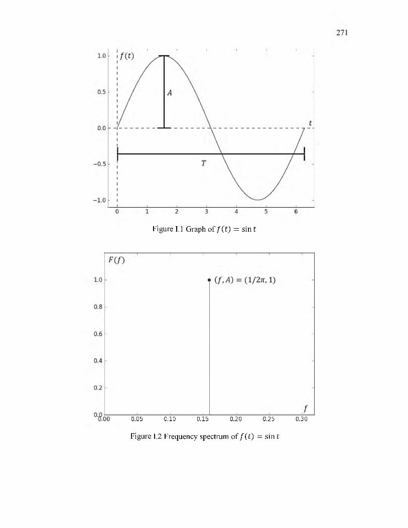
Figure I.1 Graph of f ( t ) = sin t

0.05 0.10 0.15 0.20 0.25 0.30

Figure I.2 Frequency spectrum of f( t ) = sin t

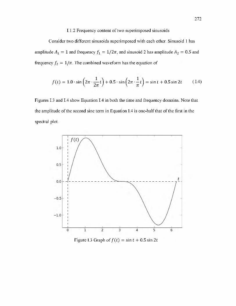
I.1.2 Frequency content of two superimposed sinusoids

Consider two different sinusoids superimposed with each other. Sinusoid 1 has

amplitude ^ = 1 and frequency / = 1 /2 ^ , and sinusoid 2 has amplitude = 0-5 and

frequency / 2 = 1/rc. The combined waveform has the equation of

/ ( t ) = 1-0 ■ sin ( 2^ ■ — t ) + 0-5 ■ sin ( 2^ ■ — t ) = sin t + 0-5 sin 2 t ( I.4)

Figures I.3 and I.4 show Equation I.4 in both the time and frequency domains. Note that

the amplitude of the second sine term in Equation I.4 is one-half that of the first in the

spectral plot.

272

Figure I.3 Graph of / ( t ) = sin t + 0-5 sin 2 t

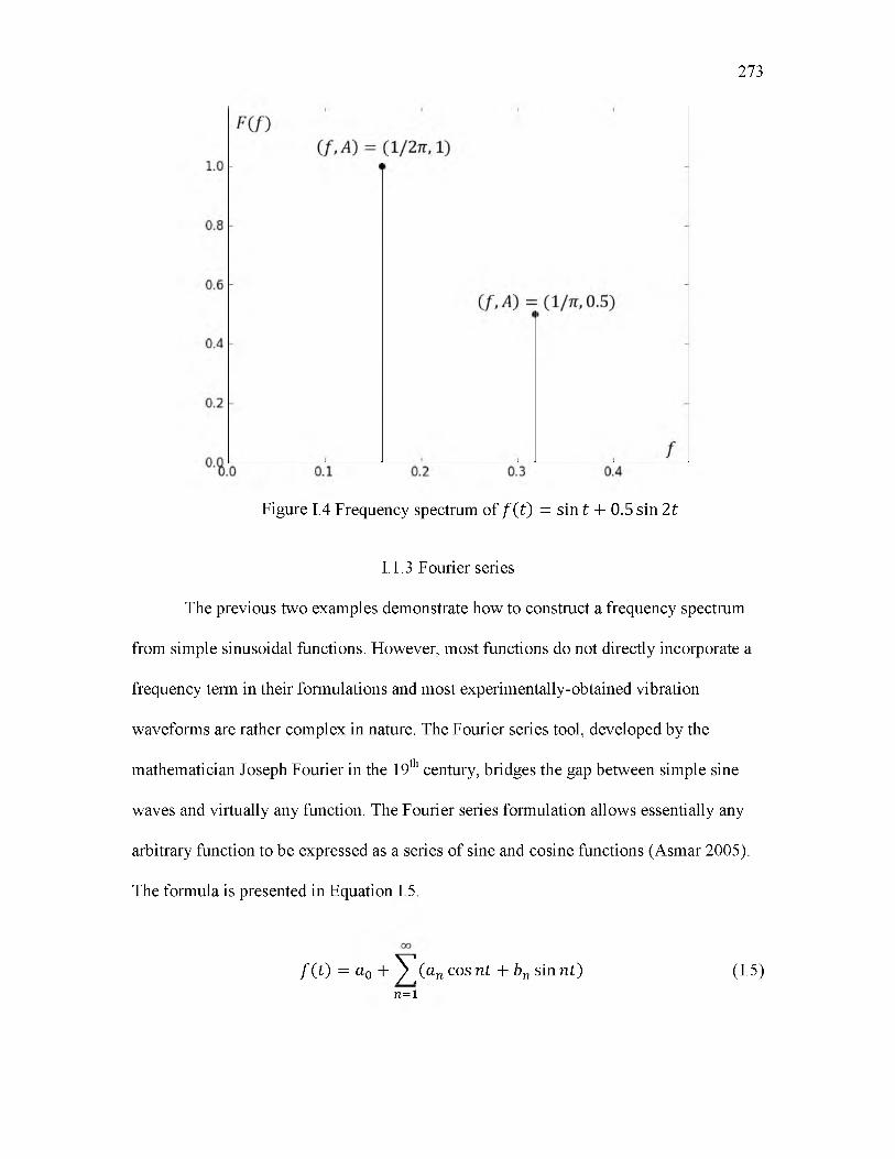
273

Figure I.4 Frequency spectrum of f ( t) = s i n t + 0 . 5 s i n 2 t

I.1.3 Fourier series

The previous two examples demonstrate how to construct a frequency spectrum

from simple sinusoidal functions. However, most functions do not directly incorporate a

frequency term in their formulations and most experimentally-obtained vibration

waveforms are rather complex in nature. The Fourier series tool, developed by the

mathematician Joseph Fourier in the 19th century, bridges the gap between simple sine

waves and virtually any function. The Fourier series formulation allows essentially any

arbitrary function to be expressed as a series of sine and cosine functions (Asmar 2005).

The formula is presented in Equation I.5.

/ ( t ) = a0 + ^ ( an cos nt + bn sin nt) ( I.5)71=1

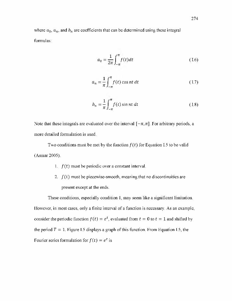
274

where a0, an, and bn are coefficients that can be determined using these integral

formulas:

a0 = r 1 j f ( t ) d t ( I.6)

1 nan = — I f ( t ) c o s n t d t ( I.7)

n J-n

1 nbn = — \ f ( t ) s i n n t d t ( I.8)

n J-n

Note that these integrals are evaluated over the interval [—n, n ] . For arbitrary periods, a

more detailed formulation is used.

Two conditions must be met by the function f ( t ) for Equation 1.5 to be valid

(Asmar 2005):

1. f { t ) must be periodic over a constant interval.

2. f { t ) must be piecewise-smooth, meaning that no discontinuities are

present except at the ends.

These conditions, especially condition 1, may seem like a significant limitation.

However, in most cases, only a finite interval of a function is necessary. As an example,

consider the periodic function f ( t ) = e t , evaluated from t = 0 to t = 1 and shifted by

the period T = 1. Figure I.5 displays a graph of this function. From Equation I.5, the

Fourier series formulation for f ( t ) = e l is

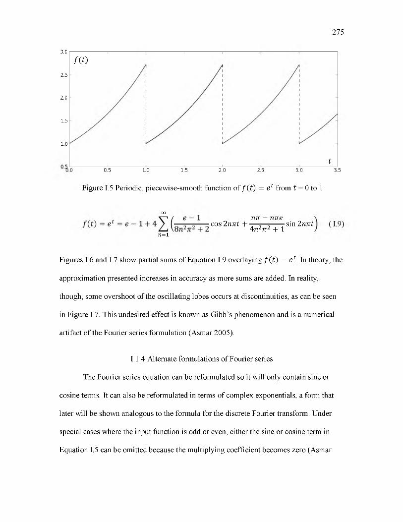
275

3.0

m

2.0

2.5

1.0

1.5

t0.5 1.0 1.5 2.0 2.5 3.0 3.5

Figure I.5 Periodic, piecewise-smooth function of f ( t) = e t from t = 0 to 1

OO

cos 2nnt +4n2n 2 + 1nn — nne

sin 2nnt71=1

Figures I.6 and I.7 show partial sums of Equation I.9 overlaying f ( t) = e t . In theory, the

approximation presented increases in accuracy as more sums are added. In reality,

though, some overshoot of the oscillating lobes occurs at discontinuities, as can be seen

in Figure I.7. This undesired effect is known as Gibb’s phenomenon and is a numerical

artifact of the Fourier series formulation (Asmar 2005).

I.1.4 Alternate formulations of Fourier series

The Fourier series equation can be reformulated so it will only contain sine or

cosine terms. It can also be reformulated in terms of complex exponentials, a form that

later will be shown analogous to the formula for the discrete Fourier transform. Under

special cases where the input function is odd or even, either the sine or cosine term in

Equation I.5 can be omitted because the multiplying coefficient becomes zero (Asmar

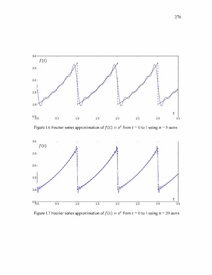
276

Figure I.6 Fourier series approximation of / ( t ) = from t = 0 to 1 using n = 5 sums

Figure I.7 Fourier series approximation of / ( t ) = from t = 0 to 1 using n = 20 sums

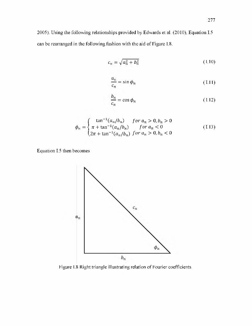
277

2005). Using the following relationships provided by Edwards et al. (2010), Equation I.5

can be rearranged in the following fashion with the aid of Figure I.8.

Cn V an bn ( I.10)

dTI— = sin (pn

— = cos <pn

( I.11)

( 1.12)

tan ~1(an/ b n) f o r an > 0, bn > 0 <pn = { n + tan _ 1 ( an/b n) f or an < 0

2̂7r + tan ~1(an/ b n) f o r an > 0, bn < 0( I13)

Equation I.5 then becomes

Figure I.8 Right triangle illustrating relation of Fourier coefficients

278

f ( t) = a0 + I cn (— c o s n t + — si n n t )-"an = 1

— a0 + I cn(sin <pn cos nt + cos <pn sin n t)n= 1

— a0 + I cn sin (n t + <pn) (1.14)71=1

To cast Equation I.5 in terms of complex exponentials, Euler’s identity must be

employed:

eint = c o s n t + j s innt (1.15)

where j = V—1 is an imaginary number. The complex exponential Fourier series is

00

f ( t) = I Cn e 1 nt ( 1.16)

1 f T/2= r l f ( 0 e Jnt d t ( 1.17)

1 J - T / 2

where T is the interval over which f ( t) is piecewise smooth. This formulation is useful in

that it shows for each frequency given by n, the corresponding magnitude of the input

function at that frequency is the constant coefficient .

I.1.5 The Fourier transform

A mathematic transform is a formula that converts a function or set of data from

one domain to another. The Fourier transform converts a continuous function or a set of

data, representing a signal in the time domain, to the frequency domain. Conversely, the

inverse Fourier transform will do the opposite. The Fourier series is a generalization of

the Fourier series that can be applied over the entire domain of a function or data set, not

just a periodic interval (Asmar 2005).

For analytical functions, the Fourier and inverse Fourier transforms are integrals

of the form

279

/O O■•j si 00

= —= I f ( t) e - -,'6J td t ( —oo < a < oo) ( 1.18)v 2 7T J—oo

■•j s i 0 0

f ( t) = —= I / ( a ) e t d t ( —oo < t < oo)v

( 1.19)

where, in applying to a waveform signal, may be considered the angular frequency.

The Fourier transform is a special case of the Laplace transform.

For discrete data, the Fourier transform is called the discrete Fourier Transform

(DFT). For a set of N points, the DFT and its inverse are given by

w - i

* [fc] = i ^ Z X W e - ( !20)71 = 0

w - i

X [n] = ^ x [fc] e '2 ̂ ( I.21)k =0

where and are indices of discrete points in the time and frequency domains,

respectively (Cha and Molinder 2006). The values of X [fc] are discrete approximations of

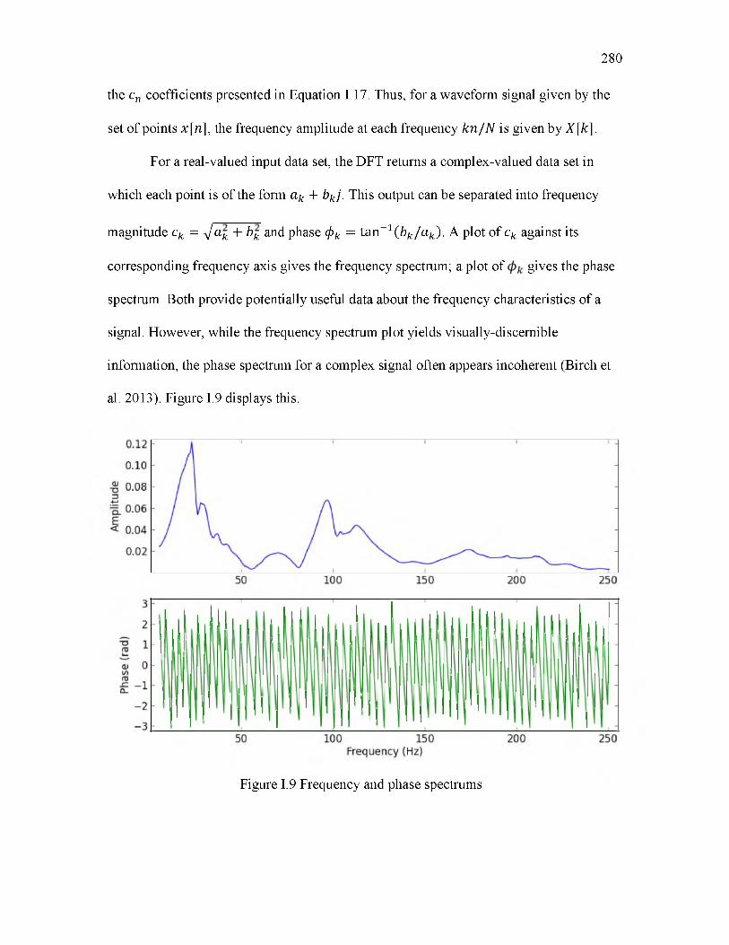
the cn coefficients presented in Equation 1.17. Thus, for a waveform signal given by the

set of points x [n] , the frequency amplitude at each frequency k n /N is given by X [k] .

For a real-valued input data set, the DFT returns a complex-valued data set in

which each point is of the form ak + bkj. This output can be separated into frequency

magnitude ck = ^ a k + bk and phase <pk = ta n _ 1 ( bk/ a k) . A plot of ck against its

corresponding frequency axis gives the frequency spectrum; a plot of gives the phase

spectrum. Both provide potentially useful data about the frequency characteristics of a

signal. However, while the frequency spectrum plot yields visually-discernible

information, the phase spectrum for a complex signal often appears incoherent (Birch et

al. 2013). Figure I.9 displays this.

280

Figure I.9 Frequency and phase spectrums

One important detail to note is the construction of the frequency axis that

corresponds with the DFT transform. Digital sampling theory dictates that the highest

measurable frequency of a signal is only one-half of the sampling frequency, or Nyquist

rate (Cha and Molinder 2006). Thus, if the sampling rate of a discrete data set is f , the

maximum measureable frequency is 0 .5 f .

The frequency terms of the DFT have a slightly unusual order. The frequencies

start at zero and climb to 0 .5 f , then suddenly drop to - 0 .5 f and climb back up to zero.

The exact order depends on whether the input data set contains an even or odd number of

values. The frequency domain arrangement, expressed mathematically for a data set with

N values, is (Cha and Molinder 2006)

281

/Even: f \n\ = —

J NN N N

0, 1, 2....- - 1, - - + 1.....-2, - 1

Odd: f [ n ] = j jN - 1 (TV — 1) (JV - 1)

0 1 2 ------------------- - ---------- - + 1 - 2 - 1V t - L , L * f . . . , , , \ . L , J_

( I.22)

( I23)

This behavior can be corrected by shifting both the frequencies and the DFT output about

the origin. However, not all applications involving signal analysis need to do this, for two

reasons. First, when only the frequency or phase spectrum is needed, only nonnegative

frequencies are useful—negative frequencies do not make any physical sense. Second,

the DFT possesses a property that if a real-valued data set is transformed, the second half

of the transformed data set is the complex conjugate of the first half. This means that the

frequency magnitudes on both sides of the origin are virtually symmetrical, although the

phases are 180° opposite. Thus, unless phases on both sides of the origin become

important, all the useful data is contained within the first half of the transformed data set.

I.1.6 The FFT algorithm

Through the use of a computer language, the DFT is easily implemented. The

formulas presented in Equations I.20 and I.21, however, have a major drawback that

becomes apparent with large data arrays. For a data set with N values, the number of

operations to compute the DFT is on the order of . This rapidly becomes inefficient for

large volumes of data. The FFT algorithm is a computationally-efficient implementation

of the DFT that can decrease the number of operations to the order of N 1 o g2 N. This

results in substantial savings with large data sets. The FFT, originally discovered in 1965

by J.W. Turkey and J.W. Cooley, is considered to be among one the most important

contributions in numerical mathematics (Asmar 2005).

A drawback to the FFT is its level of complexity. The underlying principle of the

FFT is to factor out “roots of unity”, or the factors e i2nk‘n l/N, where kt and n are

specific indices shared by a group of values within the larger data body (Asmar 2005).

The difficulty lies in determining how to factor out these roots with an arbitrarily-sized

data set. The mathematics and logic involved can become rather complicated. The

simplest way to compute the FFT is to only accept data sets that contain 2 m points, with

m being arbitrary. Certain shortcuts can then be taken in the FFT formulation, reducing

complexity and increasing computational speed. FFT algorithms that employ this

approach are termed radix-2 FFTs. Constraining the size of the input data array to a

power of 2 may seem like a ridiculous limitation, but as will be shown in the next section,

a technique called zero padding can be employed to bring any data set to the necessary

size.

282

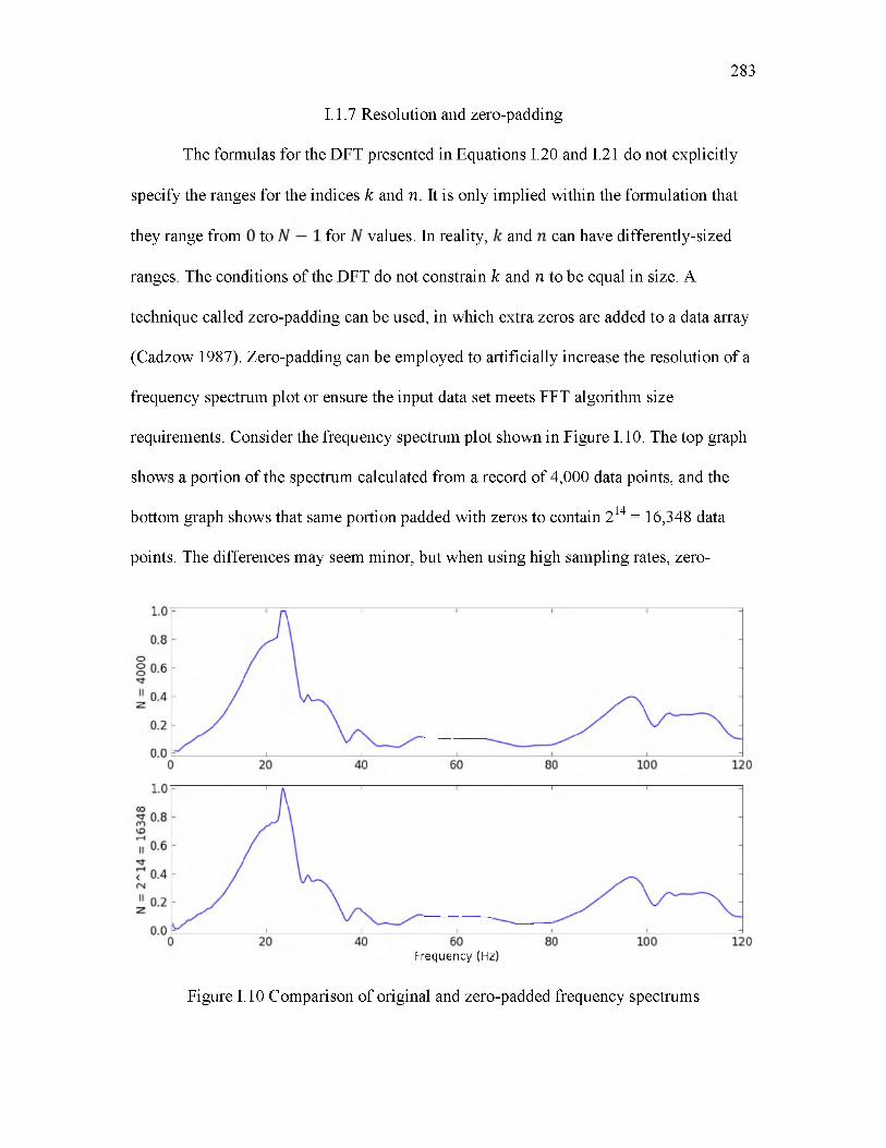
I.1.7 Resolution and zero-padding

The formulas for the DFT presented in Equations I.20 and I.21 do not explicitly

specify the ranges for the indices k and n. It is only implied within the formulation that

they range from to for values. In reality, and can have differently-sized

ranges. The conditions of the DFT do not constrain k and n to be equal in size. A

technique called zero-padding can be used, in which extra zeros are added to a data array

(Cadzow 1987). Zero-padding can be employed to artificially increase the resolution of a

frequency spectrum plot or ensure the input data set meets FFT algorithm size

requirements. Consider the frequency spectrum plot shown in Figure I.10. The top graph

shows a portion of the spectrum calculated from a record of 4,000 data points, and the

bottom graph shows that same portion padded with zeros to contain 214 = 16,348 data

points. The differences may seem minor, but when using high sampling rates, zero-

283

Frequency (Hz)

Figure I.10 Comparison of original and zero-padded frequency spectrums

padding can be beneficial for analyzing lower frequency patterns in sharper detail. Care

must be taken when zero-padding, though, as high-frequency artifacts can sometimes

appear in the spectrum.

If zero-padding is needed in order to reach a size requirement of 2 m data points,

the following formula can be used. For a data array of values, the minimum power

to raise 2 to such that is greater than equals

284

mIn .V

In 2(I24)

where [ ] is the ceiling function.

I.1.8 Windowing and spectral leakage

Sometimes when a frequency spectrum is computed from a set of experimentally

measured data, a large frequency magnitude will appear near 0 Hz. Usually this is a

numerical artifact from the Fourier transform. A key assumption in Fourier analysis with

finite data sets (or functions on a finite interval) is that the input data set repeats itself

periodically. If the endpoints of the data set do not meet at the same amplitude, the

Fourier transform assumes that a discontinuity has occurred and thus calculates a

frequency value at a frequency approximately equal to the reciprocal of the duration of

the input data set. This is the lowest frequency on the frequency axis. As an example,

observe the periodic functions in Figures I.11 and 1.12. Figure I.11 has no discontinuities

and thus will not generate a large spike near 0 Hz. Figure I.12, on the other hand, has a

large discontinuity that will be accounted for in the Fourier transform.

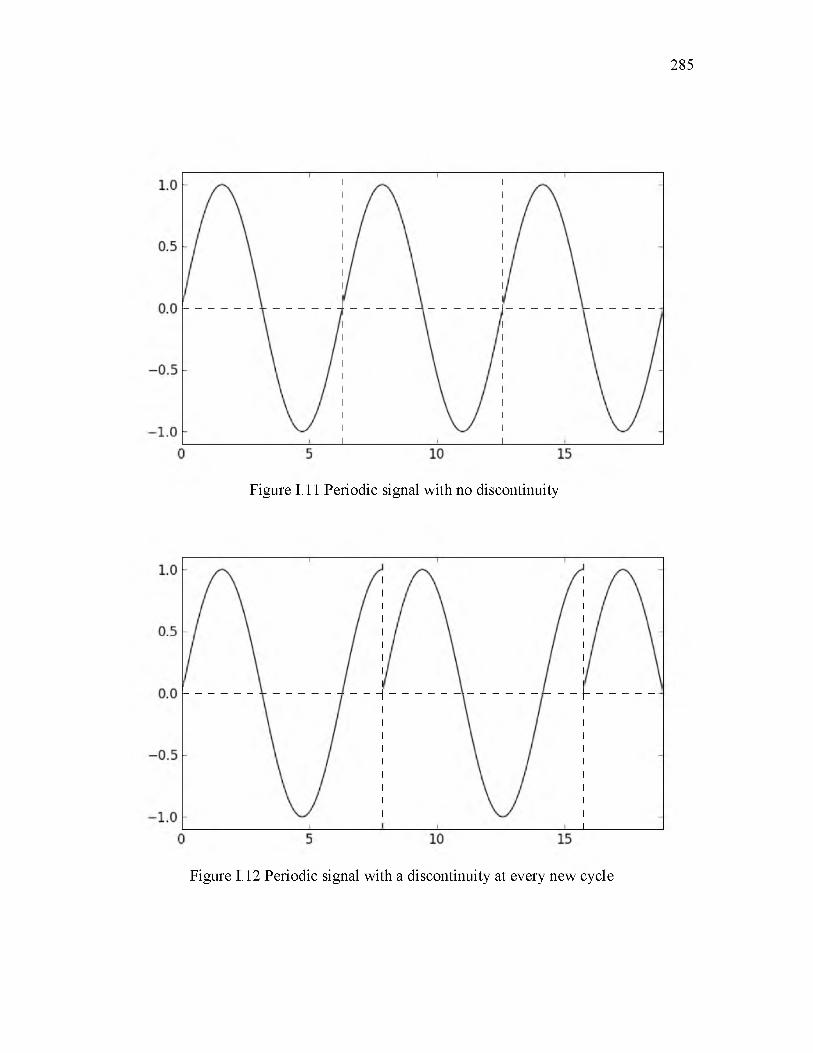
285

Figure I.11 Periodic signal with no discontinuity

Figure I.12 Periodic signal with a discontinuity at every new cycle

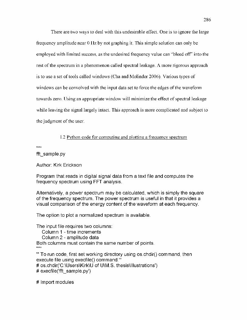
286

There are two ways to deal with this undesirable effect. One is to ignore the large

frequency amplitude near 0 Hz by not graphing it. This simple solution can only be

employed with limited success, as the undesired frequency value can “bleed o ff’ into the

rest of the spectrum in a phenomenon called spectral leakage. A more rigorous approach

is to use a set of tools called windows (Cha and Molinder 2006). Various types of

windows can be convolved with the input data set to force the edges of the waveform

towards zero. Using an appropriate window will minimize the effect of spectral leakage

while leaving the signal largely intact. This approach is more complicated and subject to

the judgment of the user.

I.2 Python code for computing and plotting a frequency spectrum

IIIIII

fft_sample.py

Author: Kirk Erickson

Program that reads in digital signal data from a text file and computes the frequency spectrum using FFT analysis.

Alternatively, a power spectrum may be calculated, which is simply the square of the frequency spectrum. The power spectrum is useful in that it provides a visual comparison of the energy content of the waveform at each frequency.

The option to plot a normalized spectrum is available.

The input file requires two columns:Column 1 - time increments Column 2 - amplitude data

Both columns must contain the same number of points.i i i i i i

''' To run code, first set working directory using os.chdir() command, then execute file using execfile() command.'''# os.chdir('C:\Users\Kirk\U of U\M.S. thesis\Illustrations')# execfile('fft_sample.py')

# Import modules

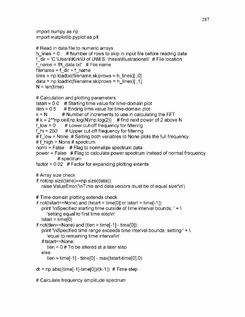
287

import numpy as np import matplotlib.pyplot as plt

# Read in data file to numeric arraysh_lines = 0 # Number of rows to skip in input file before reading dataf_dir = 'C:\Users\Kirk\U of U\M.S. thesis\Illustrations\\' # File locationf_name = 'fft_data.txt' # File namefilename = f_dir + f_nametime = np.loadtxt(filename,skiprows = h_lines)[:,0]data = np.loadtxt(filename,skiprows = h_lines)[:,1]N = len(time)

# Calculation and plotting parameterststart = 0.0 # Starting time value for time-domain plottlen = 0.5 # Ending time value for time-domain plotk = N # Number of increments to use in calculating the FFT# k = 2**np.ceil(np.log(N)/np.log(2)) # find next power of 2 above N f_low = 0 # Lower cut-off frequency for filteringf_hi = 250 # Upper cut-off frequency for filtering# f_low = None # Setting both variables to None plots the full frequency# f_high = None # spectrumnorm = False # Flag to normalize spectrum datapower = False # Flag to calculate power spectrum instead of normal frequency

# spectrumfactor = 0.02 # Factor for expanding plotting extents

# Array size checkif not(np.size(time)==np.size(data)):

raise ValueError('\nTime and data vectors must be of equal size!\n')

# Time-domain plotting extends checkif not(tstart==None) and (tstart < time[0] or tstart > time[-1]):

print '\nSpecified starting time outside of time interval bounds; ' + \'setting equal to first time step\n'

tstart = time[0] if not(tlen==None) and (tlen > time[-1] - time[0]):

print '\nSpecified time range exceeds time interval bounds; setting ' + \'equal to remaining time interval\n'

if tstart==None: tlen = 0 # To be altered at a later step

else:tlen = time[-1] - time[0] - max(tstart-time[0],0)

dt = np.abs((time[-1]-time[0])/(k-1)) # Time step

# Calculate frequency amplitude spectrum

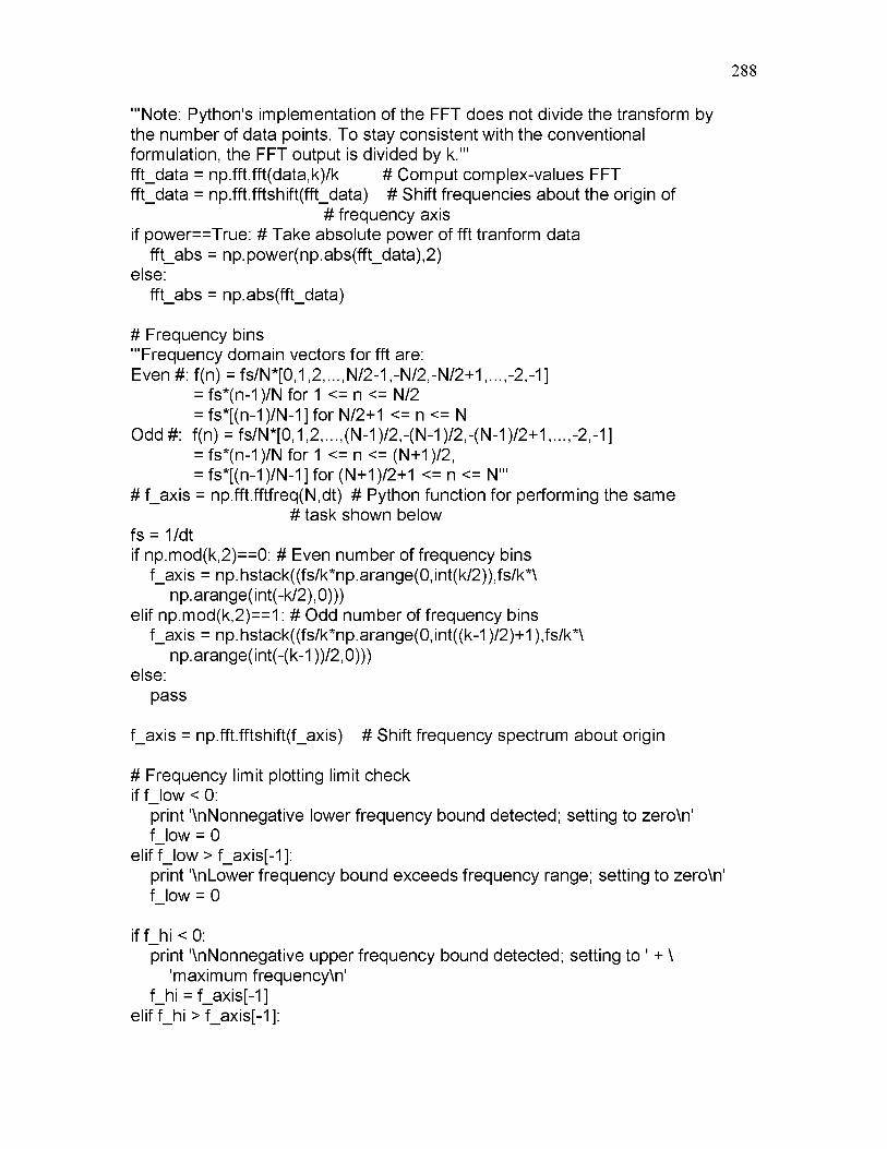
288

'''Note: Python's implementation of the FFT does not divide the transform by the number of data points. To stay consistent with the conventional formulation, the FFT output is divided by k.''' fft_data = np.fft.fft(data,k)/k # Comput complex-values FFT fft_data = np.fft.fftsh ift(fft_data) # Shift frequencies about the origin of

# frequency axis if power==True: # Take absolute power of fft tranform data

fft_abs = np.power(np.abs(fft_data),2) else:

fft_abs = np.abs(fft_data)

# Frequency bins'''Frequency domain vectors for fft are:Even #: f(n) = fs/N*[0,1,2,...,N/2-1,-N/2,-N/2+1,...,-2,-1]

= fs*(n-1 )/N for 1 <= n <= N/2 = fs*[(n-1)/N-1] for N/2+1 <= n <= N

Odd #: f(n) = fs/N*[0,1,2,...,(N-1)/2,-(N-1)/2,-(N-1)/2+1,...,-2,-1]= fs*(n-1 )/N for 1 <= n <= (N+1)/2,= fs*[(n-1 )/N-1 ] for (N+1 )/2+1 <= n <= N'''

# f_axis = np.fft.fftfreq(N,dt) # Python function for performing the same# task shown below

fs = 1 /dtif np.mod(k,2)==0: # Even number of frequency bins

f_axis = np.hstack((fs/k*np.arange(0,int(k/2)),fs/k*\ np.arange(int(-k/2),0)))

elif np.mod(k,2)==1: # Odd number of frequency bins f_axis = np.hstack((fs/k*np.arange(0,int((k-1)/2)+1),fs/k*\

np.arange(int(-(k-1 ))/2,0)))else:

pass

f_axis = np.fft.fftshift(f_ax is) # Shift frequency spectrum about origin

# Frequency limit plotting limit check if f_low < 0:

print '\nNonnegative lower frequency bound detected; setting to zero\n' f_low = 0

elif f_low > f_axis[-1]:print '\nLower frequency bound exceeds frequency range; setting to zero\n' f_low = 0

if f_hi < 0:print '\nNonnegative upper frequency bound detected; setting to ' + \

'maximum frequency\n' f_hi = f_axis[-1]

elif f_hi > f_axis[-1]:

289

print '\nUpper frequency bound exceeds frequency range; setting to ' + \ 'maximum frequency\n'

f_hi = f_axis[-1]

if f_low > f_hi:print '\nLower frequency bound greater than upper frequency bound; ' + \

'switching bounds\n' f_low,f_hi = f_hi,f_low

# Determine plotting extents for time-domain plot based on user-specified# start time and durationif not(tstart==None): # Ensure that tstart and tlen are floating point types

tstart = np.float(tstart) if not (tlen==None):

tlen = np.float(tlen)

if tstart==None:tstart = time[0] # Set starting time to first value of time array if not

# specified if tlen==None or tlen<=0:

print '\nCannot use negative or zero-length time range; setting equal ' + \'to remaining time interval\n'

tlen = time[-1] - time[0] - max(tstart-time[0],0) # Set time plot length to# the remainder of the time array if not specified or is less than or# equal to zero

# Determine plotting extents for frequency spectrum based on user-specified# frequency limitsif not(f_low==None): # Ensure that f_low and f_hi are floating point types

f_low = np.float(f_low) if not(f_hi==None):

f_hi = np.float(f_hi)

if f_low==None or f_low==0:f_p1 = f_axis.searchsorted(0) + 1 # Determine array index of origin f_low = 0.0

else:f_p1 = f_axis.searchsorted(f_low) # Determine array index of f_low

if f_hi==None: f_p2 = k-1 f_hi = f_axis[-1]

else:f_p2 = f_axis.searchsorted(f_hi) # Determine array index of f_hi

# Normalize data if specified, set plotting axes extends of frequency spectrum

# and vertical axis label if norm==False:

f_range = np.amax(fft_abs[f_p1:f_p2+1]) fr_axis = (f_low,f_hi,-factor*f_range,(1.0+factor)*f_range) ylabel2 ='Amplitude'

else:fr_axis = (f_low,f_hi,-factor,(1.0+factor))fft_abs = fft_abs/np.amax(fft_abs) # Normalize fft transform data ylabel2='Relative amplitude'

# Plot resultsplt.subplot(2,1,1) # Time domain plot of signal plt.plot(time,data,'k')plt.title('Signal and frequency spectrum') plt.xlabel('Time (sec)') plt.ylabel('Amplitude')plt.axis('tight') # Set axes extents to tightly fit datap_axis = np.asarray(plt.axis()) # Modify axes extends to slightly expandrange1 = tlenrange2 = p_axis[3] - p_axis[2] p_axis[0] = tstart - factor*range1 p_axis[2] -= factor*range2 p_axis[1] = tstart + (1.0+factor)*range1 p_axis[3] += factor*range2 plt.axis(tuple(p_axis))

plt.subplot(2,1,2) # Frequency spectrum plotplt.plot(f_axis[f_p1 :f_p2+1 ],fft_abs[f_p1 :f_p2+1 ],'b')plt.xlabel('Frequency (Hz)')plt.ylabel(ylabel2)plt.axis(fr_axis)

mng = plt.get_current_fig_manager() # Maximize figure windowmng.window.showMaximized()plt.show()

290

REFERENCES

Abo-Zena, A.M. 1977. Radiation from a finite cylindrical explosive source. Geophys. 42(7):1384-1393.

Adams, D.J., Gay, N.C., and Cross, M. 1993. Preconditioning - A technique forcontrolling rockbursts. In Rockbursts and Seismicity in Mines 93. Edited by R.P. Young. Brookfield, VT: A.A. Balkema. pp. 29-33.

Adamson, W.R., and Scherpenisse, C.R. 1998. The measurement and control of blast induced damage of final pit walls in open pit mining. In Proceedings of the Fourteenth Annual Conference on Explosives and Blasting Research, New Orleans, LA, February 8-11. Cleveland, OH: International Society of Explosives Engineers. pp. 539-555.

AEMC Instruments. 2004. What is a TDR? Chauvin Arnoux Group.http://www.aemc.com/techinfo/appnotes/CableTesters/APP-CableTesters- WhatIsATDR. Accessed May 2013.

AEMC Instruments. 2011a. Fault Mapper Pro Telephone/Coaxial/Parallel Cable Tester Graphical TDR Model CA7026. Chauvin Arnoux Group. http://www.aemc.com/ products/pdf/2127.81.pdf. Accessed May 2013.

AEMC Instruments. 2011b. User manual for CA7026 Fault Mapper Pro. Chauvin Arnoux Group. http://www.chauvin-arnoux.us/pdfs aemc/user-manuals/CA7026 EN ES PO.pdf Accessed May 2013.

Alvarez-Vigil, A.E., Gonzalez-Nicieza, C., Lopez Gayarre, F., and Alvarez-Fernandez, M.I. 2012. Predicting blasting propagation velocity and vibration frequency using artificial neural networks. Int. J. RockMech. Min. Sci. 55(2012):108-116.

Anderson, D., Ott, K., Campo, D., and Haq, S. 2004. Strain and peak particle velocity as vibration criteria: Some thoughts. In Proceedings o f the Thirtieth Annual Conference on Explosives and Blasting Technique, Vol. 2, New Orleans, LA, February 1-4. Cleveland, OH: International Society of Explosives Engineers. pp. 133-145.

Andrieux, P., McKenzie, C., Heilig, J., and Drolet, A. 1994. The impact of blasting of excavation design - A geomechanics approach. In Proceedings o f the Tenth Annual Conference on Explosives and Blasting Research, Austin, TX, January 30-February 3. Cleveland, OH: International Society of Explosives Engineers. pp.

292

Arora, S., and Dey, K. 2013. Comparison of two near-field blast vibration estimationmodels: A theoretical study. In Rock Fragmentation by Blasting - Fragblast 10. Edited by P.K. Singh and A. Sinha. Boca Raton, FL: CRC Press. pp. 465-471.

Asmar, N.H. 2005. Partial Differential Equations with Fourier Series and Boundary Value Problems. Upper Saddle River, NJ: Pearson Education, Inc.

Atchison, T.C., and Pugliese, J.M. 1964. Comparative studies o f explosives in granite - third series o f tests. Report of Investigation RI-6693. Washington, DC: U.S. Bureau of Mines.

Atchison, T.C., and Roth, J. 1961. Comparative studies o f explosives in marble. Report of Investigation RI-5797. Washington, DC: U.S. Bureau of Mines.

Atchison, T.C., and Tournay, W.E. 1959. Comparative studies o f explosives in granite. Report of Investigation RI-5509. Washington, DC: U.S. Bureau of Mines.

Atchison, T.C., Duvall, W.I., and Pugliese, J.M. 1964. Effect o f decoupling on explosion­generated strain pulses in rock. Report of Investigation RI-6333. Washington,DC: U.S. Bureau of Mines.

Atlas Powder Company. 1987. Explosives and Rock Blasting. Dallas, TX: Explosives company.

Badger, A.A., Beecroft, A.D., and Stienstra, A. 1990. Seismic data recording: Thelimiting component. Presented at the 1990 Annual Meeting for the Society of Exploration Geophysicists, September 23-27, San Francisco, CA.

Banadaki, M.M.D. 2010. Stress-wave induced fracture in rock due to explosive action. Ph.D. dissertation, University of Toronto, ON.

Bastante, F.G., Alejano, L., and Gonzalaz-Cao, J. 2012. Predicting the extent of blast- induced damage in rock masses. Int. J. RockMech. Min. Sci. 56(2012):44-53.

Birch, W.J., Bermingham, L., Hosein, S, White, T.J., and Farnfield, R. 2013. Phase - The forgotten problem of blast vibration prediction. In Rock Fragmentation by Blasting - Fragblast 10. Edited by P.K. Singh and A. Sinha. Boca Raton, FL:CRC Press. pp. 425-432.

Blair, D.P. 1987. The measurement, modelling, and control of ground vibrations due to blasting. In Second International Symposium on Rock Fragmentation by Blasting, Keystone, CO, August 23-26. Edited by W.L. Fourney and R.D. Dick. Bethel,CT: Society for Experimental Mechanics. pp. 88-101.

Blair, D., and Minchinton, A. 1996. On the damage zone surrounding a single blasthole.In Rock Fragmentation by Blasting - Fragblast-5. Edited by B. Mohanty.

107-119.

293

Brookfield, VT: A.A. Balkema. pp. 21-130.

Blair, D.P., and Spathis, A.T. 1982. Attenuation of explosion-generated pulse in rock masses. J. Geophys. Res. 87(B5):3885-3892.

Bollinger, G.A. 1971. Blast Vibration Analysis. Carbondale, IL: Southern Illinois University Press.

Born, W.T. 1941. The attenuation constant of earth materials. Geophys. 6(2):132-148.

Bradley, W. Jr., and Eller, E.E. 1961. Introduction to shock and vibration measurements. In Shock and Vibration Handbook. Vol. 1, Basic Theory and Measurements. Edited by C.M. Harris and C.E. Crede. New York: McGraw-Hill.

Brent, G.F., and Smith, G.E. 1996. Borehole pressure measurements behind blast limits as an aid to determining the extent of rock damage. In Rock Fragmentation by Blasting - Fragblast-5. Edited by B. Mohanty. Brookfield, VT: A.A. Balkema. p p .103-112.

Brent, G.F,. and Smith, G.E. 1999. The detection of blast damage by borehole pressure measurement. In Sixth International Symposium for Rock Fragmentation by Blasting - Fragblast 6. Johannesburg, Republic of South Africa: The South African Institute of Mining and Metallurgy. pp. 9-13.

Brinkman, J.R. 1990. An experimental study of the effects of shock and gas penetration in blasting. Third International Symposium on Rock Fragmentation by Blasting, Brisbane, Australia, August 26-31. Brisbane, Qld., Australia: The Australasian Institute of Mining and Metallurgy. pp. 55-66.

Cadzow, J.A. 1987. Foundations o f Digital Signal Processing and Data Analysis. New York: Macmillan.

Cha, P.D., and Molinder, J.I. 2006. Fundamentals o f Signals and Systems. New York: Cambridge University Press.

Cho, S., Ogata, Y., and Kaneko, K. 2003. Strain-rate dependency of the dynamic tensile strength of rock. Int. J. RockMech. Min. Sci. 40(5):763-777.

Curbach, M., and Eibl, J. 1990. Crack velocity in concrete. Eng. Fract. Mech. 35(1- 3):321-326.

Darling, P. 2011. Mining: Ancient, modern, and beyond. In SMEMining EngineeringHandbook, 3rd ed. Vol. 1. Edited by P. Darling. Littleton, CO: Society for Mining, Metallurgy, and Exploration.

Davidson, L. 2008. Fundamentals o f Shock Wave Propagation in Solids. Berlin: Springer-Verlag.

294

Dehghani, H., and Ataee-pour, M. 2011. Development of a model to predict peak particle velocity in a blasting operation. Int. J. RockMech. Min. Sci. 48(1):51—58.

Devine, J.F., Beck, R.H., Meyer, A.V.C., and Duvall, W.I. 1965. Vibration levelstransmitted across a presplit fracture plane. Report of Investigation RI-6695. Washington, DC: U.S. Bureau of Mines.

Dey, K., and Murthy, V.M.S.R. 2013. Monitoring ground vibrations for predictingoverbreak threshold levels in underground drivages. In Rock Fragmentation by Blasting - Fragblast 10. Edited by P.K. Singh and A. Sinha. Boca Raton, FL: CRC Press. pp. 787-791.

Dowding, C.H. 1985. Blast Vibration Monitoring and Control. Englewood Cliffs, NJ: Prentice-Hall, Inc.

Dowding, C.H., and Aimone, C.T. 1992. Rock breakage: Explosives. In SME Mining Engineering Handbook, 2nd ed. Vol. 1. Edited by H.L. Hartman. Littleton, CO: Society for Mining, Metallurgy, and Exploration.

Drukovanyi, M.F., Kravtsov, V.S., Chernyavskii, Y.E., Shelenok, V.V., Reva, N.P., and Zver’kov, S.N. 1976. Calculation of fracture zones created by exploding cylindrical charges in ledge rocks. J. Min. Sci. 12(3):292-295.

Duvall, W.I., and Petkof, B. 1959. Spherical propagation o f explosion-generated strain pulses in rock. Report of Investigation RI-5483. Washington, DC: U.S. Bureau of Mines.

Dyno Nobel. n.d. DYNOMIX. http://www.dynonobel.com/files/2010/04/1Dynomix.pdf. Accessed May 2013.

Edwards, C.G., Penney, D.E., and Calvis, D. 2010. Differential Equations and Linear Algebra, 3rd ed. Upper Saddle River, NJ: Pearson Prentice Hall.

Faber, K., and Maxwell, P.W. 1997. Geophone spurious frequency: What is it and how does it affect seismic data quality? Can. J. Explor. Geophys. 33(1-2):46-54.

Farnfield, R.A. 1996. So you think you are monitoring peak particle velocity. InProceedings o f the Twelfth Symposium on Explosives and Blasting Research, Orlando, FL, February 4-8. Cleveland, OH: International Society of Explosives Engineers. pp. 13-20.

Favreau, R.F. 1969. Generation of strain waves in rock by an explosion in a spherical cavity. J. Geophys. Res. 74(17):4267-4280.

Floyd, J. 2008. Efficient Blasting Techniques. Course notes. Blast Dynamics, Inc.

Fogelson, D.E., Duvall, W.I., and Atchison, T.C. 1959. Strain energy in explosion­generated strain pulses. Report of Investigation RI-5514. Washington, DC: U.S.

295

Bureau of Mines.

Furtney, J.K., Cundall, P.A., and Chitombo, G.P. 2010. Development in numericalmodeling of blast induced rock fragmentation: Updates from the HSBM project. In Rock Fragmentation by Blasting - Fragblast 9. Edited by J.A. Sanchidrian. New York: CRC Press. pp. 355-342.

Geospace Technologies. 2012. GS-20DM. http://www. geospace.com/tag/ gs-20dm/. Accessed April 2013.

Gohkle, C. n.d. Unofficial Windows binaries for Python extension packages. http://www.lfd.uci.edu/~gohlke/pythonlibs/. Accessed May 2013.

Graizer, V.M. 1979. Determination of true ground displacement by using strong motion records. Izvestiya Phys. Solid Earth. 15(12):875-885.

Hagedoorn, A.L., Kruithof, E.J., and Maxwell, P.W. 1988. A practical set of guidelines for geophone element testing and evaluation. First Break. 6(10):325-331.

Hamdi, E., Audiguier, M., Mauza, J., and Fjader, K. 2003. Blast induced micro cracks assessment in muckpile blocks: P-wave velocity and porosity measurements. In Proceedings of the EFEE Second World Conference on Explosives and Blasting Technique, Prague, Czech Republic, September 10-12. Edited by R. Holmberg. Lisse, The Nethelands: A.A. Balkema. pp. 389-399.

Hamdi, E., Romdhanea, N.B., and Le Cleac’h, J.M. 2011. A tensile damage model for rocks: Application to blast induced damage assessment. Comput. Geotech. 38(2):133-141.

Harries, G. 1983. The modelling of long cylindrical charges of explosive. In Proceedings o f the First International Symposium on Rock Fragmentation by Blasting, Lulea, Sweden, August 23-26. Edited by R. Holmberg and A. Rustan. Lulea, Sweden: Lulea, University of Technology. pp. 419-431.

Heelan, P.A. 1953. Radiation from a cylindrical source of finite length. Geophys. 18(3):685-696.

Herrmann, W. 1969. Constitutive equation for the dynamic compaction of ductile porous materials. J. Appl. Phys. 40(6):2490-2499.

Hinzen, K.G. 1998. Comparison of seismic and explosive energy in five smooth blasting test rounds. Int. J. RockMech. Min. Sci. 35(7):957-967.

Hoffman, J.E. 2003. A search for alternative electronic order in the high temperature superconductor Bi2Sr2CaCu2O8+s by scanning tunneling microscopy. Ph.D. dissertation, University of California, Berkeley, CA. p.136.

Holcomb, D.J., Stone, C.M., and Costin, L.S. 1990. Combining acoustic emission

296

locations and a microcrack damage model to study development of damage in brittle materials. In Rock Mechanics Contributions and Challenges: Proceedings of the 31st U.S. Symposium. Edited by W.A. Hustrulid and G.A. Johnson. Brookfield, VT: A.A. Balkema. pp. 645-651.

Hustrulid, W. 1999. Blasting Principles for Open Pit Mining. Vol. 2: Theoretical Foundations. Brookfield, VT: A.A. Balkema.

Hustrulid, W., and Johnson, J. 2008. A gas pressure-based drift round blast designmethodology. Washington, DC: National Institute for Occupational Safety and Health.

Hustrulid, W., and Lu, W. 2002. Some general design concepts regarding the control of blast-induced damage during rock slope excavation. In Rock Fragmentation by Blasting - Fragblast 7. Edited by W. Xuguang. Beijing, China: Metallurgical Industry Press. pp. 95-100.

Hustrulid, B., Iverson, S., Furtney, J., Cundall, P., and Torres, M. 2009. Developments in the numerical modeling of rock blasting: Updates from the HSBM project. Presented at the 2009 Annual Meeting and Exhibit of the Society for Mining, Metallurgy, and Exploration, Denver, CO, February 22-25, 2009.

International Society of Explosives Engineers. 2011. Fragmentation and heave process.In ISEE Blasters’ Handbook, 18th ed. Edited by J.F. Stiehr. Cleveland, OH: ISEE.

Iverson, S.R., Hustrulid, W.A., Johnson, J.C., Tesarik, D., and Akbarzadeh, Y. 2010. The extent of blast damage from a fully coupled explosive charge. In Rock Fragmentation by Blasting - Fragblast 9. Edited by J.A. Sanchidrian. New York: CRC Press. pp. 459-468.

Iverson, S., Kerkering, C., and Hustrulid, W. 2008. Application of the NIOSH-Modified Holmberg-Persson approach to perimeter blast design. Washington, DC: National Institute for Occupational Safety and Health. http://www.cdc.gov/niosh/mining/ UserFiles/works/pdfs/aotnm.pdf. Accessed March 2012.

Jimeno, C.L., Jimeno, E.L., and Carcedo, F.J.A. 1995. Drilling and Rock Blasting. Geomining Technological Institute of Spain. Brookfield, VT: A.A. Balkema.

Johnson, J.C. 2010. The Hustrulid bar - A dynamic strength test and its application to the cautious blasting of rock. Ph.D. dissertation, University of Utah, Salt Lake City, UT.

Johnson, G.R., and Holmquist, T.J. 1993. An improved computational constitutive model for brittle materials. In High-Pressure Science and Technology - 1993, Colorado Springs, CO, June 28-July 2. American Institute of Physics. pp. 981-984.

Jordan, D.W. 1962. The stress wave from a finite cylindrical explosive. J. Math. Mech. 11(4):503-552.

297

Katsabanis, P.D. 2001. Applications of numerical modeling to examine damage in wall control operations. In Proceedings o f the Twenty-Seventh Annual Conference on Explosives and Blasting Technique, Vol. 2, Orlando, FL, January 28-31. Cleveland, OH: International Society of Explosives Engineers. pp. 25-37.

Katsabanis, P.D. 2005. Application of air decking to blasting - Findings from numerical modelling. In Proceedings o f the Thirty-First Annual Conference on Explosives and Blasting Technique, Vol. 1, Orlando, FL, February 6-9. Cleveland, OH: International Society of Explosives Engineers. pp. 217-228.

Kelsall, P.C., Case, J.B., and Chabannes, C.R. 1984. Evaluation of excavation-induced changes in rock permeability. Int. J. Rock Mech. Min. Sci. Geomech. Abstr. 21(3):123-135.

Khandelwai, M., and Singh, T.N. 2009. Prediction of blast-induced ground vibration using artificial neural network. Int. J. Rock Mech. Min. Sci. 46(7):1214-1222.

Kilebrant, M., Norrgard, T., and Jem, M. 2010. The size of the damage zone in relation to the linear charge concentration. In Rock Fragmentation by Blasting - Fragblast 9. Edited by J.A. Sanchidrian. New York: CRC Press. pp. 449-457.

Kim, D.S., and McCarter, M.K. 1993. Assessment of damage in rock subjected toexplosive loading. In Proceedings o f the Ninth Annual Symposium on Explosives and Blasting Research, San Diego, CA, January 31-February 4. Cleveland, OH: International Society of Explosives Engineers. pp. 163-177.

Kjartansson, E. 1979. Constant Q-wave propagation and attenuation. J. Geophys. Res. 84(B9):4737-4748.

Kolsky, H. 1963. Stress Waves in Solids. Mineola, NY: Dover Publications, Inc.

LeBlanc, T.M., Ryan, J.M., and Heilig, J.H. 1996. Predicting the envelope of damage from the detonation of a confined charge. In Proceedings o f the Twenty-Second Annual Conference on Explosives and Blasting Technique, Vol. 2, Orlando, FL, February 4-8. Cleveland, OH: International Society of Explosives Engineers. pp. 11-31.

Lee, E.L., Hornig, H.C., and Kury, J.W. 1968. Adiabatic expansion of high explosive detonation products. UCRL-50422. Lawrence Radiation Laboratory, University of California, Livermore.

Liu, L., and Katsabanis, P.D. 1997. Development of a continuum damage model for blasting analysis. Int. J. Rock Mech. Min. Sci. 34(2):217-231.

Liu, Q., Hung, T., Counter, D., and Andrieux, P. 1998. A case study of blast damage evaluation in open stope mining at Kidd Creek Mines. In Proceedings o f the Fourteenth Annual Conference on Explosives and Blasting Research, New Orleans, LA, February 8-11. Cleveland, OH: International Society of Explosives

298

Engineers. pp. 323-336.

Lizotte, Y.C. 1996. Controlled blasting at the CANMET experimental mine. Min. Eng. 48(6):74-78.

Lu, P., and Latham, J.P. 1999. Investigation into the relationship between fractaldimension and the blastability of rock masses. In Sixth International Symposium for Rock Fragmentation by Blasting - Fragblast 6. Johannesburg, Republic of South Africa: The South African Institute of Mining and Metallurgy. pp. 191­198.

Lundborg, N. 1972. A statistical theory of the polyaxial compressive strength of materials. Int. J. RockMech. Min. Sci. Geomech. Abstr. 9(5):617-624.

McHugh, S. 1983. Crack extension caused by internal gas pressure compared with extension caused by tensile stress. Int. J. Fract. 21(3):163-176.

McKenzie, C.K. 1999. A review of the influences of gas pressure on block stability during rock blasting. In EXPLO ’99. Edited by C. Workman-Davies. Carlton, Vic., Australia: The Australasian Institute of Mining and Metallurgy. pp. 173­179.

McKenzie, C.K., and Holley, K.G. 2004. A study of damage profiles behind blasts. In Proceedings o f the Thirtieth Annual Conference on Explosives and Blasting Technique, Vol. 2, New Orleans, LA, February 1-4. Cleveland, OH: International Society of Explosives Engineers. pp. 203-214.

McKown, A. 1986. Perimeter control blasting for underground excavations in fractured and weathered rock. Bull. Assoc. Eng. Geol. 23(4):461-478.

Mencacci, S., and Farnfield, R. 2003. The measurement and analysis of near-fieldpressure transients in production blasting. In Proceedings o f the EFEE Second World Conference on Explosives and Blasting Technique, Prague, Czech Republic, September 10-12. Edited by R. Holmberg. Lisse, The Nethelands: A.A. Balkema. pp. 467-473.

Meyer, R., Kohler, J., and Homburg, A. 2002. Explosives, 5th ed. Weinheim, Germany: Wiley-VCH Verlag GmbH & Co. KGaA.

Micro-Measurements. 2010. Strain gauge selection: Criteria, procedures,recommendations. Vishay Precision Group. http://www.vishaypg.com/docs/ 11055/tn505.pdf. Accessed April 2013.

Mohammadnejad, M., Gholami, R., Sereshki, F., and Jamshidi, A. 2013. A newmethodology to predict backbreak in blasting operation. Int. J. Rock Mech. Min. Sci. 60(2013):75-81.

Monjezi, M., Rezaei, M., and Yazdian, A. 2009. Prediction of backbreak in open-pit

299

blasting using fuzzy set theory. Expert Syst. Appl. 37(3):2637-2643.

Montgomery, D.C., and Runger, G.C. 2007. Applied Statistics and Probability for Engineers, 4th ed. Hoboken, NJ: John Wiley & Sons, Inc.

Murthy, V.M.S.R., Dey, K., and Mohanty, P.R.. 2004. Predicting tunnel overbreak thresholds from acceleration measurements - An Indian case study. In Proceedings o f the Thirtieth Annual Conference on Explosives and Blasting Technique, Vol. 2, New Orleans, LA, February 1-4. Cleveland, OH: International Society of Explosives Engineers. pp. 389-399.

National Oceanic and Atmospheric Administration (NOAA). n.d. How hydrodynamic models are used. http://www.nauticalcharts.noaa.gov/csdl/learn models.html. Accessed March 2012.

Neiman, I.B. 1979. Determination of dimensions of the zone of crushing of rock in place by blasting. J. Min. Sci. 15(5):480-485.

Neiman, I.B. 1983. Mathematical model of the explosive action of a fracturing charge in a ledge rock mass. J. Min. Sci. 19(6):494-499.

Neiman, I.B. 1986. Volume models of the action of cylindrical-charge explosion in rock. J. Min. Sci. 22(6):455-463.

Nicholls, H.R., Johnson, C.F., and Duvall, W.I. 1971. Blasting vibrations and their effects on structures. Bulletin 656. Washington, DC: U.S. Bureau of Mines.

Onederra, I., Chitombo, G.P., Cundall, P.A., and Furtney, J.K. 2010. Towards a complete validation of the lattice scheme in the Hybrid Stress Blasting Model (HSBM). In Rock Fragmentation by Blasting - Fragblast 9. Edited by J.A. Sanchidrian. New York: CRC Press. pp. 343-351.

Onederra, I., Furtney, J.K., and Sellers, E. 2013a. Modelling the extent of damage from fully coupled explosive charges. In Rock Fragmentation by Blasting - Fragblast 10. Edited by P.K. Singh and A. Sinha. Boca Raton, FL: CRC Press. pp. 267-274.

Onederra, I., Furtney, J.K., Sellers, E., and Iverson, S. 2013b. Modelling blast induced damage from a fully coupled explosive charge. Int. J. RockMech. Min. Sci. 58(2013):73-84.

Oriard, L.L. 1972. Blasting effects and their control in open pit mining. In Geotechnical Practice for Stability in Open Pit Mining: Proceedings o f the Second International Conference on Stability in Open Pit Mining, Vancouver, BC, November 1-2. Ann Arbor, MI: Bell Howell Information and Learning Co.

Oriard, L.L. 1982. Blasting effects and their control. In Underground Mining Methods Handbook. Edited by W.A. Hustrulid. New York, NY: Society for Mining, Metallurgy, and Exploration. pp. 1590-1603.

300

Ouchterlony, F. 1995. Review of rock blasting and explosives engineering research at SveBeFo. In EXPLO ’95. Carlton, Vic., Australia: The Australasian Institute of Mining and Metallurgy. pp. 133-146.

Ouchterlony, F. 1997. Prediction of crack lengths in rock after cautious blasting with zero inter-hole delay. Int. J. Blasting and Fragmentation. 1(4):417-444.

Ouchterlony, F., Nie, S., Nyberg, U., and Deng, J. 1996. Monitoring of large open cutrounds by VOD, PPV and gas pressure measurements. In Rock Fragmentation by Blasting - Fragblast-5. Edited by B. Mohanty. Brookfield, VT: A.A. Balkema. pp. 167-176.

Ouchterlony, F., Nyberg, U., Olsson, M., Bergqvist, I., Granlund, L., and Grind, H. 2004. Where does the explosive energy in rock blasting rounds go? Sci. Technol. Energetic Mater. 65(2):54-63.

Ouchterlony, F., Olsson, M., and Bergqvist, I. 2001. Towards new Swedishrecommendations for cautious perimeter blasting. In EXPLO 2001. Edited by A. Marton. Carlton, Vic., Australia: The Australasian Institute of Mining and Metallurgy. pp. 169-181.

Ouchterlony, F., Sjoberg, C., and Jonsson, B.A. 1993. Blast damage predictions fromvibration measurements at the SKB underground laboratories at Aspo in Sweden. In Proceedings o f the Ninth Annual Symposium on Explosives and Blasting Research, San Diego, CA, January 31-February 4. Cleveland, OH: International Society of Explosives Engineers. pp. 189-197.

Pariseau, W.G. 2007a. Design Analysis in Rock Mechanics. Philadelphia, PA: Taylor and Francis. pp. 473-501.

Pariseau, W.G. 2007b. Fitting failure criteria to laboratory strength tests. Int. J. Rock Mech. Min. Sci. 44(2007):637-646.

Park, D., and Jeon, S. 2010. Reduction of blast-induced vibration in the direction oftunneling using an air-deck at the bottom of a blasthole. Int. J. Rock Mech. Min. Sci. 47(5):752-761.

Paventi, M., Lizotte, Y., Scoble, M., and Mohanty, B. 1996. Measuring rock massdamage in drifting. In Rock Fragmentation by Blasting - Fragblast-5. Edited by B. Mohanty. Brookfield, VT: A.A. Balkema. pp. 131-138.

PCB Piezotronics. 2002. Model 353B32 - Installation and operating manual.http://www.pcb.com/contentstore/docs/PCB Corporate/Vibration/Products/Manu als/353B32.pdf. Accessed November 2012.

PCB Piezotronics. 2013. Introduction to Piezoelectric Accelerometers. http://www.pcb.com/techsupport/. Accessed May 2013.

301

PCB Piezotronics. 2013. General piezoelectric theory.http://www.pcb.com/TechSupport/tech gen#.UcJyUJwyyxg. Accessed May 2013.

Persson, P.A., Holmberg, R., and Lee, J. 1994. Rock Blasting and Explosives Engineering. Boca Raton, FL: CRC Press, Inc.

Peterson, J.A. 2001. Blast damage mechanisms at Ekati™ Mine. M.Sc. thesis, University of Alberta, Edmonton, AB.

Prasad, U. 2000. Dynamic fracture characteristics of selected rocks. Ph.D. dissertation, McGill University, Montreal, QC.

Preece, D.S., and Chung, S.H. 2003. Blast induced rock fragmentation prediction using the RHT constitutive model for brittle materials. In Proceedings o f the Twenty- Ninth Annual Conference on Explosives and Blasting Technique, Vol. 2, Nashville, TN, February 2-5. Cleveland, OH: International Society of Explosives Engineers. pp. 375-381.

Preece, D.S., and Lownds, C.M. 2008. 3D computer simulation of bench blasting with precise delay timing. In Proceedings o f the Thirty-Fourth Annual Conference on Explosives and Blasting Technique, Cleveland, OH, January 27-30. Cleveland, OH: International Society of Explosives Engineers. pp. 191-200.

Pusch, R., and Stanfors, R. 1996. Disturbance of rock around blasted tunnels. In RockFragmentation by Blasting - Fragblast-5. Edited by B. Mohanty. Brookfield, VT: A.A. Balkema. pp. 153-159.

Python Software Foundation. 2013. About Python. http://www.python.org/about/. Accessed May 2013.

Qian, W.Z., and Hui, L. 1997. A fractal and damage model for rock-breaking by blasting. In Proceedings o f the Twenty-Third Annual Conference on Explosives and Blasting Technique, Las Vegas, NV, February 2-5. Cleveland, OH: International Society of Explosives Engineers. pp. 327-331.

Rathore, S.S., Jain, S.C., and Parik, S. 2013. ANN approach for blast vibration control in limestone quarry. In Rock Fragmentation by Blasting - Fragblast 10. Edited by P.K. Singh and A. Sinha. Boca Raton, FL: CRC Press. pp. 495-500.

Riedel, W., Thoma, K., Hiermaier, S., and Schmolinske, E. 1999. Penetration ofreinforced concrete by BETA-B-500 numerical analysis using a new macroscopic concrete model for hydrocodes. In Proceedings o f the 9th International Symposium on the Interaction o f the Effects o f Munitions with Structures, Berlin- Strausberg, Germany, March 3-7.

Rorke, A.J., and Milev, A.M. 1999. Near field vibration monitoring and associated rock damage. In Sixth International Symposium for Rock Fragmentation by Blasting -

302

Fragblast 6. Johannesburg, Republic of South Africa: The South African Institute of Mining and Metallurgy. pp. 19-22.

Rosenthal, M.F., and Morlock, G.L. 1987. Blasting Guidance Manual. Washington, DC: Office of Surface Mining Reclamation and Enforcement. http://www.osmre.gov/ lrg/docs/directive315.pdf. Accessed April 2011.

Russel, D.A. 2013. Longitudinal and transverse wave motion. Pennsylvania StateUniversity. http://www.acs.psu.edu/drussell/Demos/waves/wavemotion.html. Accessed March 2013.

Ryu, C.H., Choi, B.H., and Jeong, J.H. 2013. Assessment of blast-induced damaged zone and its control. In Rock Fragmentation by Blasting - Fragblast 10. Edited by P.K. Singh and A. Sinha. Boca Raton, FL: CRC Press. pp. 725-730.

Sanchidrian, J.A., Segarra, P., and Lopez, L.M. 2007. Energy components in rock blasting. Int. J. RockMech. Min. Sci. 44(1):130-147.

Scoble, M.J., Lizotte, Y.C., Paventi, M., and Mohanty, B.B. 1997. Measurement of blast damage. Min. Eng. 49(6):103-108.

Scott, J.H., Lee, F.T., Carroll, R.D., and Robinson, C.S. 1968. The relationship ofgeophysical measurements to engineering and construction parameters in the Straight Creek tunnel pilot bore, Colorado. Int. J. Rock Mech. Min. Sci. Geomech. Abstr. 5(1):1 -30.

Segarra, P., Sanchidrian, J.A., Lopez, L.M., and Llamas, A. 2013. Measurement errors in vibrations from blasting. In Rock Fragmentation by Blasting - Fragblast 10. Edited by P.K. Singh and A. Sinha. Boca Raton, FL: CRC Press. pp. 349-356.

Seto, M., Nag, D.K., and Vutukuri, V.S. 1996. Evaluation of rock mass damage usingacoustic emission technique in the laboratory. In Rock Fragmentation by Blasting- Fragblast-5. Edited by B. Mohanty. Brookfield, VT: A.A. Balkema. pp. 139­145.

Singer, J.A., Link, C.A., and Iverson, S.R. 2010. High resolution seismic refraction tomography for determining depth of blast induced damage in a mine wall. J. Explos. Eng. 27(1):34-43.

Singh, S.P., and Lamond, R.D. 1993. Investigation of blast damage and underground stability. In Proceedings o f the 12th Conference on Ground Control in Mining, Morgantown, WV, August 3-5. pp. 366-372.

Singh, T.N., Dontha, L.K., and Bhardwaj, V. 2008. Study into blast vibration and frequency using ANFIS and MVRA. Min. Technol. 117(3):116-121.

Siskind, D.E., Stagg, M.S., Kopp, J.W., and Dowding, C.H. 1980. Structure response and damage produced by ground vibration from surface mine blasting. Report of

303

Investigation RI-8507. Washington, DC: U.S. Bureau of Mines.

Smith, A.A. 2003. A modified Holmberg-Persson approach to predict blast damage. M.S. thesis, University of Utah, Salt Lake City, UT.

Spathis, A.T. 1999. On the energy efficiency of blasting. In Sixth InternationalSymposium for Rock Fragmentation by Blasting - Fragblast 6. Johannesburg, Republic of South Africa: The South African Institute of Mining and Metallurgy. pp. 81-90.

Spathis, A.T., Blair, D.P., and Grant, J.R. 1987. Blast damage assessment of rock by using the high frequency cross hole seismic method. In Second International Symposium on Rock Fragmentation by Blasting, Keystone, CO, August 23-26. Edited by W.L. Fourney and R.D. Dick. Bethel, CT: Society for Experimental Mechanics. pp. 488-497.

Starfield, A.M., and Pugliese, J.M. 1968. Compression waves generated in rock bycylindrical explosive charges: A comparison between a computer model and field measurements. Int. J. Rock Mech. Min. Sci. 5(1):65-77.

Stewart, I. 2002. Does God Play Dice? The New Mathematics o f Chaos, 2nd ed. Malden, MA: Blackwell Publishing. pp. 201-227.

Sun, C. 2013. Damage zone prediction for rock blasting. Ph.D. dissertation, University of Utah, Salt Lake City, UT.

Sutherland, M. 1990. Improving mine safety through perimeter blasting at Inco Limited's Thompson T-3 mine. Can. Inst. Min. Metall. Pet. Bull. 83(940):45-48.

Tawardrous, A.S., Preece, D.S., and Gelnville, J.P. 2013. Modification of the RHT model for enhanced tensile response predictions of geological materials. In Rock Fragmentation by Blasting - Fragblast 10. Edited by P.K. Singh and A. Sinha. Boca Raton, FL: CRC Press. pp. 309-323.

Tose, S.S.J. 2006. A review of the design criteria and practical aspects of developing a successful pre-split. In Stability o f Rock Slopes in Open Pit Mining and Civil Engineering Situations. Johannesburg, Republic of South Africa: The South African Institute of Mining and Metallurgy. pp. 525-546.

Trivino, L.F., and Mohanty, B. 2013. Estimation of blast-induced damage through cross­hole seismometry in single-hole blasting experiments. In Rock Fragmentation by Blasting - Fragblast 10. Edited by P.K. Singh and A. Sinha. Boca Raton, FL: CRC Press. pp. 685-695.

U.S. Gypsum Corporation. 1999. Hydro-Stone® gypsum cement. http://www.usg.com/rc/ data-submittal-sheets/industrial-plasters-cements/hydrostone/hydro-stone-gypsum-cement-data-en-IG1379.pdf. Accessed January 2013.

304

Wang, R., Schurr, B., Milkereit, C., Shao, Z., and Jin, M. 2011. An improved automatic scheme for empirical baseline correction of digital strong-motion records. Bull. Seismol. Soc. Am. 101(5):2029-2044.

Wheeler, R. 2004. The importance of proper seismometer coupling. In Proceedings o f the Thirtieth Annual Conference on Explosives and Blasting Technique, Vol. 2, New Orleans, LA, February 1-4. Cleveland, OH: International Society of Explosives Engineers. pp. 147-160.

Xia, K., Huang, S., and Jha, A.K. 2010. Dynamic tensile test of coal, shale and sandstone using split Hopkinson pressure bar: a tool for blast and impact assessment. Int. J. Geotech. Earthquake Eng. 1(2):24-37.

Yang, R., and Ray, K. 2013. A method to determine 3-D dynamic strain tensor based on displacement gradients from blast vibration and field test results. In Rock Fragmentation by Blasting - Fragblast 10. Edited by P.K. Singh and A. Sinha. Boca Raton, FL: CRC Press. pp. 341-348.

Yang, R., and Scovira, S. 2010. A model for near and far field blast vibration based on multiple seed waveforms and transfer functions. In Proceedings o f the Thirty- Sixth Annual Conference on Explosives and Blasting Technique, Vol. 2, Orlando, FL, January 7-10. Cleveland, OH: International Society of Explosives Engineers. pp. 223-242.

Yang, J., and Wang, S. 1996. A new constitutive model for rock fragmentation byblasting - fractal damage model. In Rock Fragmentation by Blasting - Fragblast- 5. Edited by B. Mohanty. Brookfield, VT: A.A. Balkema. pp. 95-100.

Yang, J., Jin, Q., and Gao, W. 2002. A new damage model for rock fragmentation by blasting based on stress wave attenuation and its application. In Rock Fragmentation by Blasting - Fragblast 7. Edited by W. Xuguang. Beijing, China: Metallurgical Industry Press. pp. 139-143.

Yang, R., Bawden, W.F., and Katsabanis, P.D. 1996. A new constitutive model for blast damage. Int. J. RockMech. Min. Sci. Geomech. Abstr. 33(3):245-254.

Yang, R.L., Rocque, P., Katsabanis, P., and Bawden, W.F. 1993. Blast damage study by measurement of blast vibration and damage in the area adjacent to blast hole. In Rock Fragmentation by Blasting - Fragblast-4. Edited by H.P. Rossmanith. Brookfield, VT: A.A. Balkema. pp. 137-144.

Zhang, J.C., and Chang, C. 1999. On damage mechanism of microcrack zone in rock blasting and its measurement. In Sixth International Symposium for Rock Fragmentation by Blasting - Fragblast 6. Johannesburg, Republic of South Africa: The South African Institute of Mining and Metallurgy. pp. 359-363.

Zhou, Y.X., Xia, K., Li, X.B., Li, H.B., Ma, G.W., Zhao, J., Zhou, Z.L., and Dai, F. 2012.

305

Suggested methods for determining the dynamic strength parameters and mode-I fracture toughness of rock materials. Int. J. RockMech. Min. Sci. 49(2012):105- 112.

Zhou, Y., and Zhoa, J. 2011. Advances in Rock Dynamics and Applications. Boca Raton, FL: CRC Press.

Zhu, Z., Mohanty B., and Xie, H. 2007. Numerical investigation of blasting-inducedcrack initiation and propagation in rocks. Int. J. Rock Mech. Min. Sci. 44(3):412- 424.

Zhu. Z., Xie, H., and Mohanty, B. 2008. Numerical investigation of blasting-induced damage in cylindrical rocks. Int. J. Rock Mech. Min. Sci. 45(2):111-121.