Investigating surface water–well interaction using stable isotope ratios of water

Investigating surface water–well interaction

using stable isotope ratios of water*

Randall J. Hunta,*, Tyler B. Coplenb, Nathaniel L. Haasc,d,David A. Saada, Mark A. Borchardtd

aUS Geological Survey, 8505 Research Lane, Middleton, WI 53562, USAbUS Geological Survey, 431 National Center, Reston, VA 20192, USA

cDepartment of Microbiology, University of Wisconsin–La Crosse, La Crosse, WI 54601, USAdMarshfield Clinic Research Foundation, 1000 N. Oak Ave, Marshfield, WI 54449, USA

Received 25 September 2003; revised 30 June 2004; accepted 9 July 2004

Abstract

Because surface water can be a source of undesirable water quality in a drinking water well, an understanding of the amount of

surface water and its travel time to the well is needed to assess a well’s vulnerability. Stable isotope ratios of oxygen in river water at

the City of La Crosse, Wisconsin, show peak-to-peak seasonal variation greater than 4‰ in 2001 and 2002. This seasonal signal was

identified in 7 of 13 city municipal wells, indicating that these 7 wells have appreciable surface water contributions and are potentially

vulnerable to contaminants in the surface water. When looking at wells with more than 6 sampling events, a larger variation in d18O

compositions correlated with a larger fraction of surface water, suggesting that samples collected for oxygen isotopic composition

over time may be useful for identifying the vulnerability to surface water influence even if a local meteoric water line is not available.

A time series of d18O from one of the municipal wells and from a piezometer located between the river and the municipal well

showed that the travel time of flood water to the municipal well was approximately 2 months; non-flood arrival times were on the

order of 9 months. Four independent methods were also used to assess time of travel. Three methods (groundwater temperature

arrival times at the intermediate piezometer, virus-culture results, and particle tracking using a numerical groundwater-flow model)

yielded flood and non-flood travel times of less than 1 year for this site. Age dating of one groundwater sample using 3H–3He methods

estimated an age longer than 1 year, but was likely confounded by deviations from piston flow as noted by others. Chloro-

fluorocarbons and SF6 analyses were not useful at this site due to degradation and contamination, respectively. This work illustrates

the utility of stable hydrogen and oxygen isotope ratios of water to determine the contribution and travel time of surface water in

groundwater, and demonstrates the importance of using multiple methods to improve estimates for time of travel of 1 year or less.

q 2004 Elsevier B.V. All rights reserved.

Keywords: Bank filtration; Hydrogen isotope ratio; Oxygen isotope ratio; Drinking water; Age dating; Temperature; Travel time; Black River

Journal of Hydrology 302 (2005) 154–172

www.elsevier.com/locate/jhydrol

0022-1694/$ - see front matter q 2004 Elsevier B.V. All rights reserved.

doi:10.1016/j.jhydrol.2004.07.010

* This article is a US Government work and is in the public domain in the USA. Any use of trade, product, or firm names is for descriptive

purposes only and does not imply endorsement by the US Government.

* Corresponding author. Fax: C1 608 821 3817.

E-mail address: [email protected] (R.J. Hunt).

http://www.elsevier.com/locate/jhydrol

R.J. Hunt et al. / Journal of Hydrology 302 (2005) 154–172 155

1. Introduction

Many communities use groundwater that is under

the influence of surface water, but surface water can

be a source of undesirable water quality. The City of

La Crosse, Wisconsin, is located adjacent to the

Mississippi River, but its drinking water source is

groundwater from the alluvial sand-gravel aquifer

underlying the city and the river. Numerical ground-

water-flow modeling (Hunt et al., 2003; Chapel et al.,

2003a) suggests that some municipal wells are

inducing surface water infiltration. Simulated capture

areas can be uncertain, however, because of model

parameter uncertainty and solution non-uniqueness

(Evers and Lerner, 1998). Independent methods of

identifying water sources can reduce the uncertainty

in the model, and the predictions that are premised on

modeling (Hunt et al., 2001).

Although the source of water is of interest when

assessing water-supply vulnerability, the time of travel

from the surface water source to the well also is

important. This information is critical for deciding the

response time for intervention, and is necessary for

assessing whether particular microbiological contami-

nants are viable/infectious when the surface water

reaches the well. For example, viruses are thought to

survive in the subsurface for times on the order of 6–12

months (Yates et al., 1985; Yates and Yates, 1988;

DeBorde et al., 1998); groundwater travel times often are

appreciably longer than 1 year. However, large gradients

and hydraulically conductive sediments (as might be

found near a municipal wellfield near a surface water

source) could result in travel times of less than 1 year

(e.g. Maloszewski et al., 1990; Hotzl et al., 1989; Sheets

et al., 2002). Thus, much could be gained if simple

methods could be used to assess time of travel to the

supply well in addition to identifying the source of water.

Stable hydrogen, oxygen, carbon, nitrogen, and

sulfur isotope ratios can be valuable tools for

investigating hydrologic systems (Mazor, 1997; Clark

and Fritz, 1997). Of these, stable hydrogen (d2H) and

oxygen isotope (primarily d18O) ratios in water are

ideal conservative tracers of water sources, because

they are part of the water molecule itself. Stable isotope

ratios of water are conservative in aquifers at low

temperature, but water can be isotopically fractionated

on the surface at less than 100% humidity (Gat, 1970).

Because the vapor pressure and diffusivity of H216O is

greater than that of H218O, the residual liquid is

characterized by a higher H218O content after evapor-

ation and rain or snow falling from clouds is enriched in

H218O, preferentially depleting air masses in H2

18O as

they move across continents. Protium (1H) and

deuterium (2H) can also fractionate, but to a greater

extent due to larger relative mass difference. 2H is also

enriched in precipitation falling from clouds, which

caused air masses to become preferentially depleted in2H as they become colder and lose their moisture.

Additionally, evaporation preferentially enriches sur-

face water in 18O relative to 2H. These processes create

a seasonal cycle in surface water such that water is

depleted in 18O and 2H in snowmelt in the winter and

early spring, and water is enriched in 18O and 2H during

summer and early fall. As a result, 18O/16O and 2H/1H

ratios can be used to identify the source and timing of

groundwater flow (e.g. Fritz, 1981; Maloszewski et al.,

1990; Krabbenhoft et al., 1990).

Whereas discrete physical measurements represent

the system at the point in time the sample was taken,

stable isotope compositions reflect the initial isotopic

composition of waters entering the system, sub-

sequent additions and withdrawals, and processes

acting within the system. Consequently, transient

hydrologic events have isotopic effects proportional to

their physical importance. Periodic monitoring of

hydraulic gradients only show ‘snapshots’ of the flow

field, but cannot relay the importance of gradient

changes (i.e. the amount of movement caused by a

reversal) without a continuous data set and rigorous

analysis. Given a sufficient understanding of the

underlying flow system and distinction between

sources, stable hydrogen and oxygen isotope ratios

of water can give similar information with reduced

sampling and physical measurement (Hunt et al.,

1998). However, approaches using stable isotopes of

water are not widely used in wellhead protection

studies and have only infrequently been applied to

drinking water supplies (for example, Stichler et al.,

1986; Maloszewski et al., 1990; Hotzl et al., 1989;

McCarthy et al., 1992; Coplen et al., 1999).

In this study, stable hydrogen and oxygen isotope

ratios of water are used to identify sources of water for

13 municipal wells in the City of La Crosse,

Wisconsin, and to assess the time of travel from

surface water to one of the municipal wells. The time

of travel was also evaluated using four independent

R.J. Hunt et al. / Journal of Hydrology 302 (2005) 154–172156

methods including: (1) commonly used age-dating

tracers, (2) virus-culture results for Hepatitis A virus

(HAV), (3) a groundwater temperature time series,

and (4) a numerical groundwater-flow model. This

study utilized relatively simple analyses that would be

readily accessible to others; it also provides insights

into potential methods for hydrologic settings where

wells are near surface water sources.

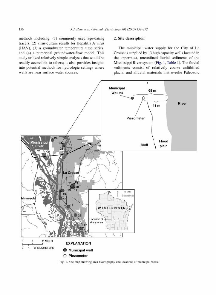
Fig. 1. Site map showing area hydrograph

2. Site description

The municipal water supply for the City of La

Crosse is supplied by 13 high capacity wells located in

the uppermost, unconfined fluvial sediments of the

Mississippi River system (Fig. 1, Table 1). The fluvial

sediments consist of relatively coarse unlithified

glacial and alluvial materials that overlie Paleozoic

y and locations of municipal wells.

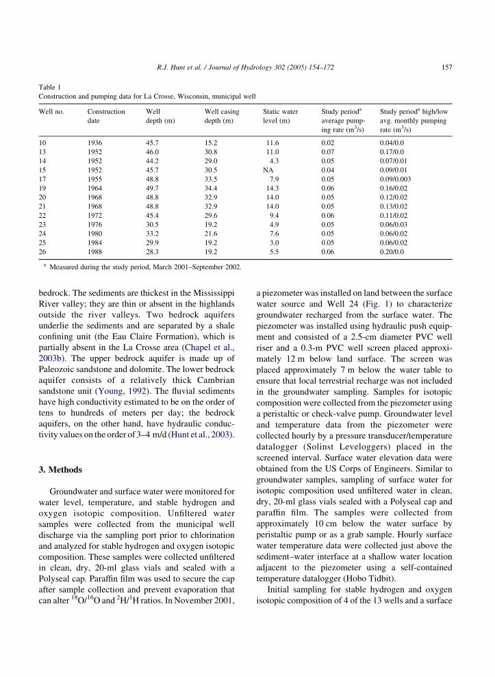
Table 1

Construction and pumping data for La Crosse, Wisconsin, municipal well

Well no. Construction

date

Well

depth (m)

Well casing

depth (m)

Static water

level (m)

Study perioda

average pump-

ing rate (m3/s)

Study perioda high/low

avg. monthly pumping

rate (m3/s)

10 1936 45.7 15.2 11.6 0.02 0.04/0.0

13 1952 46.0 30.8 11.0 0.07 0.17/0.0

14 1952 44.2 29.0 4.3 0.05 0.07/0.01

15 1952 45.7 30.5 NA 0.04 0.09/0.01

17 1955 48.8 33.5 7.9 0.05 0.09/0.003

19 1964 49.7 34.4 14.3 0.06 0.16/0.02

20 1968 48.8 32.9 14.0 0.05 0.12/0.02

21 1968 48.8 32.9 14.0 0.05 0.13/0.02

22 1972 45.4 29.6 9.4 0.06 0.11/0.02

23 1976 30.5 19.2 4.9 0.05 0.06/0.03

24 1980 33.2 21.6 7.6 0.05 0.06/0.02

25 1984 29.9 19.2 3.0 0.05 0.06/0.02

26 1988 28.3 19.2 5.5 0.06 0.20/0.0

a Measured during the study period, March 2001–September 2002.


bedrock. The sediments are thickest in the Mississippi

River valley; they are thin or absent in the highlands

outside the river valleys. Two bedrock aquifers

underlie the sediments and are separated by a shale

confining unit (the Eau Claire Formation), which is

partially absent in the La Crosse area (Chapel et al.,

2003b). The upper bedrock aquifer is made up of

Paleozoic sandstone and dolomite. The lower bedrock

aquifer consists of a relatively thick Cambrian

sandstone unit (Young, 1992). The fluvial sediments

have high conductivity estimated to be on the order of

tens to hundreds of meters per day; the bedrock

aquifers, on the other hand, have hydraulic conduc-

tivity values on the order of 3–4 m/d (Hunt et al., 2003).

3. Methods

Groundwater and surface water were monitored for

water level, temperature, and stable hydrogen and

oxygen isotopic composition. Unfiltered water

samples were collected from the municipal well

discharge via the sampling port prior to chlorination

and analyzed for stable hydrogen and oxygen isotopic

composition. These samples were collected unfiltered

in clean, dry, 20-ml glass vials and sealed with a

Polyseal cap. Paraffin film was used to secure the cap

after sample collection and prevent evaporation that

can alter 18O/16O and 2H/1H ratios. In November 2001,

a piezometer was installed on land between the surface

water source and Well 24 (Fig. 1) to characterize

groundwater recharged from the surface water. The

piezometer was installed using hydraulic push equip-

ment and consisted of a 2.5-cm diameter PVC well

riser and a 0.3-m PVC well screen placed approxi-

mately 12 m below land surface. The screen was

placed approximately 7 m below the water table to

ensure that local terrestrial recharge was not included

in the groundwater sampling. Samples for isotopic

composition were collected from the piezometer using

a peristaltic or check-valve pump. Groundwater level

and temperature data from the piezometer were

collected hourly by a pressure transducer/temperature

datalogger (Solinst Leveloggers) placed in the

screened interval. Surface water elevation data were

obtained from the US Corps of Engineers. Similar to

groundwater samples, sampling of surface water for

isotopic composition used unfiltered water in clean,

dry, 20-ml glass vials sealed with a Polyseal cap and

paraffin film. The samples were collected from

approximately 10 cm below the water surface by

peristaltic pump or as a grab sample. Hourly surface

water temperature data were collected just above the

sediment–water interface at a shallow water location

adjacent to the piezometer using a self-contained

temperature datalogger (Hobo Tidbit).

Initial sampling for stable hydrogen and oxygen

isotopic composition of 4 of the 13 wells and a surface


water site was conducted monthly from March

2001–February 2002. Based upon the results of this

preliminary sampling, isotope sampling was extended

to include the piezometer, one additional surface water

site near the piezometer, and the entire municipal well

system. These additional samples were collected

periodically during November 2001–September 2002.

Oxygen isotope ratios were measured using CO2–

H2O equilibration (Epstein and Mayeda, 1953). Stable

hydrogen isotope ratios were determined by H2–H2O

equilibration (Coplen et al., 1991). Oxygen and

hydrogen isotopic results are reported in per mill (‰)

relative to VSMOW (Vienna Standard Mean Ocean

Water) and normalized (Coplen, 1994) on scales such

that the oxygen and hydrogen isotopic values of SLAP

(Standard Light Antarctic Precipitation) are K55.5 and

K428‰, respectively. Analytical error (2s) is estimated

at G0.2 and G2.0‰ for d18O and d2H, respectively.

Water samples were collected for sulfur hexa-

fluoride (SF6) analysis from municipal wells (2 samp-

lings) and the piezometer (1 sampling) using

procedures outlined by the USGS (2003a). Water

samples collected from the piezometer also were

analyzed for chlorofluorocarbons (CFCs) and tritium–

helium (3H–3He) to determine an age of the water.

Water samples from the surface water source were

also analyzed for CFCs (1 sampling). CFC samples

were flame sealed in borosilicate-glass ampules using

equipment and procedures described by Busenberg

and Plummer (1992). Sampling protocol for 3H–3He

are detailed by USGS (2003b). Dissolved gas samples

were used to estimate recharge temperature. All age-

dating and dissolved gas samples from locations other

than municipal wells were collected using a stainless

steel and Teflon bladder pump with sample lines

constructed of copper and Viton (trademark).

SF6 and CFC samples were analyzed at the USGS

CFC laboratory in Reston, Virginia. SF6 concen-

trations were measured by gas chromatography using

an electron capture detector (Busenberg and Plum-

mer, 2000). CFC concentrations were determined in

the laboratory using a purge-and-trap gas chromato-

graphic procedure and an electron capture detector.

Details of the analytical procedure for CFCs are given

by Busenberg and Plummer (1992). CFC samples

were collected in sets of five; replicate samples were

analyzed for all sites sampled and the average value

was used. 3H–3He samples were collected in duplicate

and were analyzed using a mass spectrometer (Ludin

et al., 1997) at the Lamont-Doherty Earth Observatory

of Columbia University, Palisades, NY.

A well sample (from Well 24) that tested positive

for HAV by reverse transcription polymerase chain

reaction (RT-PCR) was analyzed by cell culture to

determine HAV infectivity (Borchardt et al., 2004).

This result is useful for determining water age because

infectious viruses in the subsurface represent travel

times on the order of 1 year or less (Yates et al., 1985;

Yates and Yates, 1988; DeBorde et al., 1998).

Negative control and positive controls were cultured

and processed simultaneously with the samples.

Positive cultures were further confirmed to contain

HAV by RT-PCR and Southern hybridization. The

reader is referred to Borchardt et al. (2004) for a

detailed description of the culture methods used.

Time of travel evaluations through groundwater-

flow modeling used the model described by Chapel

et al. (2003a). The groundwater-flow modeling code

was MODFLOW (McDonald and Harbaugh, 1988),

and the advective particle tracking code was MOD-

PATH (Pollock, 1994).

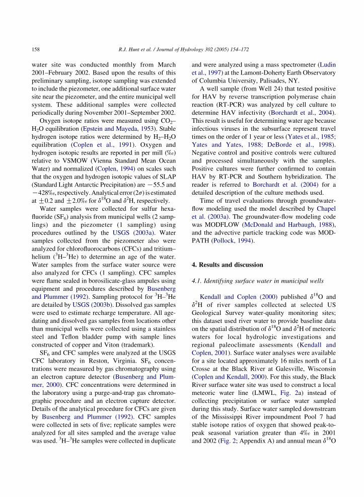
4. Results and discussion

4.1. Identifying surface water in municipal wells

Kendall and Coplen (2000) published d18O and

d2H of river samples collected at selected US

Geological Survey water-quality monitoring sites;

this dataset used river water to provide baseline data

on the spatial distribution of d18O and d2H of meteoric

waters for local hydrologic investigations and

regional paleoclimate assessments (Kendall and

Coplen, 2001). Surface water analyses were available

for a site located approximately 16 miles north of La

Crosse at the Black River at Galesville, Wisconsin

(Coplen and Kendall, 2000). For this study, the Black

River surface water site was used to construct a local

meteoric water line (LMWL, Fig. 2a) instead of

collecting precipitation or surface water sampled

during this study. Surface water sampled downstream

of the Mississippi River impoundment Pool 7 had

stable isotope ratios of oxygen that showed peak-to-

peak seasonal variation greater than 4‰ in 2001

and 2002 (Fig. 2; Appendix A) and annual mean d18O

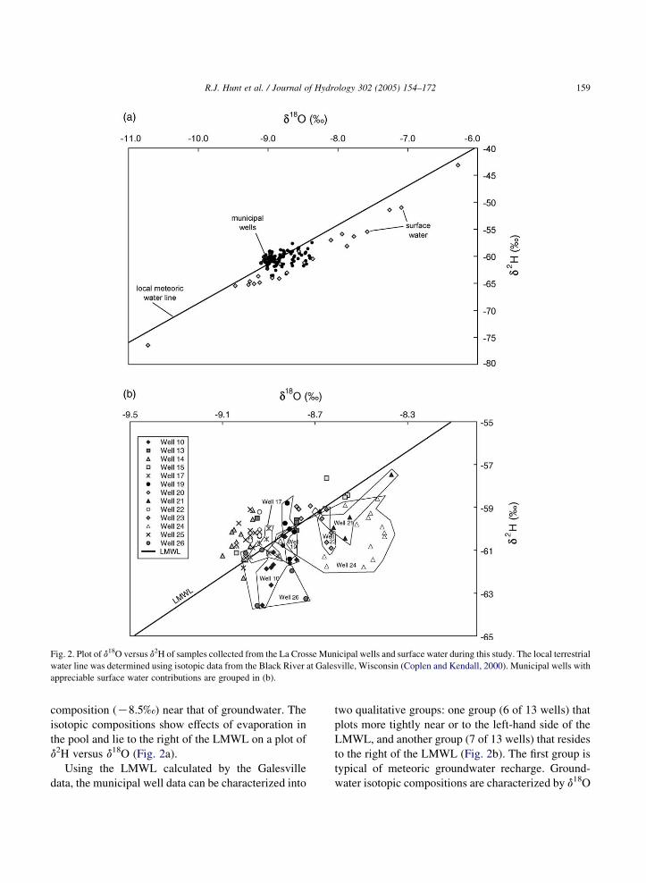
Fig. 2. Plot of d18O versus d2H of samples collected from the La Crosse Municipal wells and surface water during this study. The local terrestrial

water line was determined using isotopic data from the Black River at Galesville, Wisconsin (Coplen and Kendall, 2000). Municipal wells with

appreciable surface water contributions are grouped in (b).


composition (K8.5‰) near that of groundwater. The

isotopic compositions show effects of evaporation in

the pool and lie to the right of the LMWL on a plot of

d2H versus d18O (Fig. 2a).

Using the LMWL calculated by the Galesville

data, the municipal well data can be characterized into

two qualitative groups: one group (6 of 13 wells) that

plots more tightly near or to the left-hand side of the

LMWL, and another group (7 of 13 wells) that resides

to the right of the LMWL (Fig. 2b). The first group is

typical of meteoric groundwater recharge. Ground-

water isotopic compositions are characterized by d18O

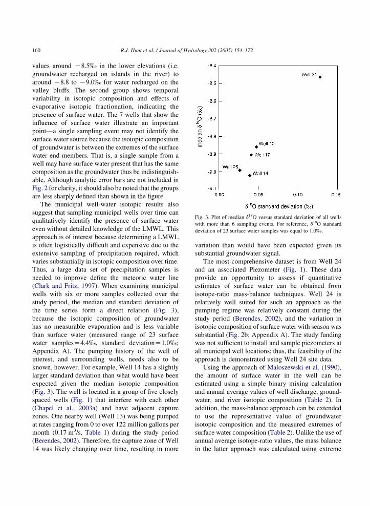
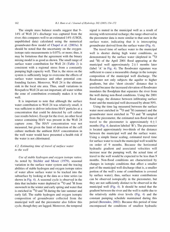
Fig. 3. Plot of median d18O versus standard deviation of all wells

with more than 6 sampling events. For reference, d18O standard

deviation of 23 surface water samples was equal to 1.0‰.


values around K8.5‰ in the lower elevations (i.e.

groundwater recharged on islands in the river) to

around K8.8 to K9.0‰ for water recharged on the

valley bluffs. The second group shows temporal

variability in isotopic composition and effects of

evaporative isotopic fractionation, indicating the

presence of surface water. The 7 wells that show the

influence of surface water illustrate an important

point—a single sampling event may not identify the

surface water source because the isotopic composition

of groundwater is between the extremes of the surface

water end members. That is, a single sample from a

well may have surface water present that has the same

composition as the groundwater thus be indistinguish-

able. Although analytic error bars are not included in

Fig. 2 for clarity, it should also be noted that the groups

are less sharply defined than shown in the figure.

The municipal well-water isotopic results also

suggest that sampling municipal wells over time can

qualitatively identify the presence of surface water

even without detailed knowledge of the LMWL. This

approach is of interest because determining a LMWL

is often logistically difficult and expensive due to the

extensive sampling of precipitation required, which

varies substantially in isotopic composition over time.

Thus, a large data set of precipitation samples is

needed to improve define the meteoric water line

(Clark and Fritz, 1997). When examining municipal

wells with six or more samples collected over the

study period, the median and standard deviation of

the time series form a direct relation (Fig. 3),

because the isotopic composition of groundwater

has no measurable evaporation and is less variable

than surface water (measured range of 23 surface

water samplesZ4.4‰, standard deviationZ1.0‰;

Appendix A). The pumping history of the well of

interest, and surrounding wells, needs also to be

known, however. For example, Well 14 has a slightly

larger standard deviation than what would have been

expected given the median isotopic composition

(Fig. 3). The well is located in a group of five closely

spaced wells (Fig. 1) that interfere with each other

(Chapel et al., 2003a) and have adjacent capture

zones. One nearby well (Well 13) was being pumped

at rates ranging from 0 to over 122 million gallons per

month (0.17 m3/s, Table 1) during the study period

(Berendes, 2002). Therefore, the capture zone of Well

14 was likely changing over time, resulting in more

variation than would have been expected given its

substantial groundwater signal.

The most comprehensive dataset is from Well 24

and an associated Piezometer (Fig. 1). These data

provide an opportunity to assess if quantitative

estimates of surface water can be obtained from

isotope-ratio mass-balance techniques. Well 24 is

relatively well suited for such an approach as the

pumping regime was relatively constant during the

study period (Berendes, 2002), and the variation in

isotopic composition of surface water with season was

substantial (Fig. 2b; Appendix A). The study funding

was not sufficient to install and sample piezometers at

all municipal well locations; thus, the feasibility of the

approach is demonstrated using Well 24 site data.

Using the approach of Maloszewski et al. (1990),

the amount of surface water in the well can be

estimated using a simple binary mixing calculation

and annual average values of well discharge, ground-

water, and river isotopic composition (Table 2). In

addition, the mass-balance approach can be extended

to use the representative value of groundwater

isotopic composition and the measured extremes of

surface water composition (Table 2). Unlike the use of

annual average isotope-ratio values, the mass balance

in the latter approach was calculated using extreme

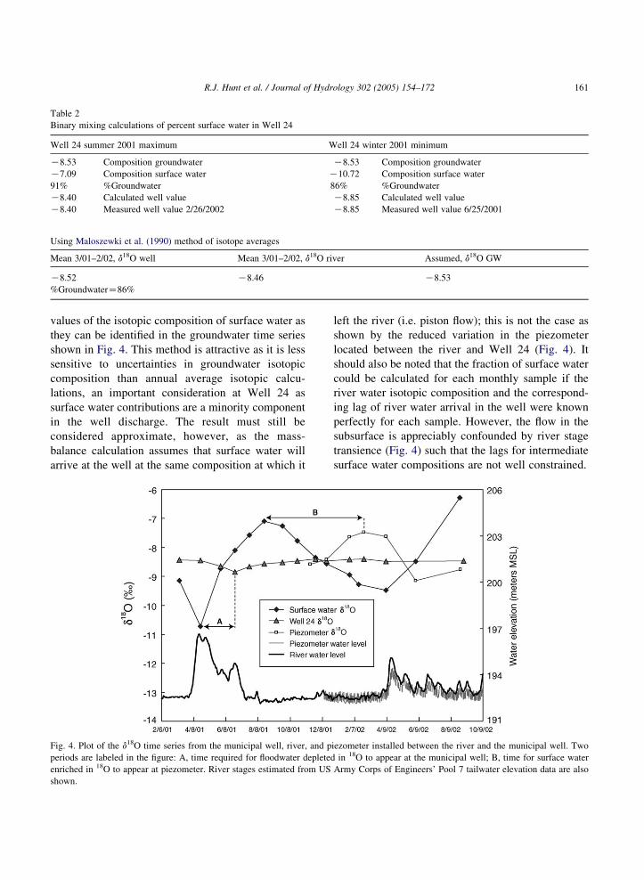
Table 2

Binary mixing calculations of percent surface water in Well 24

Well 24 summer 2001 maximum Well 24 winter 2001 minimum

K8.53 Composition groundwater K8.53 Composition groundwater

K7.09 Composition surface water K10.72 Composition surface water

91% %Groundwater 86% %Groundwater

K8.40 Calculated well value K8.85 Calculated well value

K8.40 Measured well value 2/26/2002 K8.85 Measured well value 6/25/2001

Using Maloszewki et al. (1990) method of isotope averages

Mean 3/01–2/02, d18O well Mean 3/01–2/02, d18O river Assumed, d18O GW

K8.52 K8.46 K8.53

%GroundwaterZ86%


values of the isotopic composition of surface water as

they can be identified in the groundwater time series

shown in Fig. 4. This method is attractive as it is less

sensitive to uncertainties in groundwater isotopic

composition than annual average isotopic calcu-

lations, an important consideration at Well 24 as

surface water contributions are a minority component

in the well discharge. The result must still be

considered approximate, however, as the mass-

balance calculation assumes that surface water will

arrive at the well at the same composition at which it

Fig. 4. Plot of the d18O time series from the municipal well, river, and p

periods are labeled in the figure: A, time required for floodwater depleted

enriched in 18O to appear at piezometer. River stages estimated from US

shown.

left the river (i.e. piston flow); this is not the case as

shown by the reduced variation in the piezometer

located between the river and Well 24 (Fig. 4). It

should also be noted that the fraction of surface water

could be calculated for each monthly sample if the

river water isotopic composition and the correspond-

ing lag of river water arrival in the well were known

perfectly for each sample. However, the flow in the

subsurface is appreciably confounded by river stage

transience (Fig. 4) such that the lags for intermediate

surface water compositions are not well constrained.

iezometer installed between the river and the municipal well. Two

in 18O to appear at the municipal well; B, time for surface water

Army Corps of Engineers’ Pool 7 tailwater elevation data are also


The simple mass balance results suggest that 9–

14% of Well 24’s discharge was captured from the

river; this compares well to an estimated 14% (USGS,

unpublished data) calculated using the numerical

groundwater-flow model of Chapel et al. (2003a). It

should be noted that the uncertainty on the oxygen-

isotope ratio measurements is 0.07‰ or more; thus, it

may be fortuitous that the agreement with the binary

mixing model is as good as shown. The small range of

surface water contribution for Well 24 (Table 2) is

consistent with a regional stress from a constantly

pumping high capacity well. That is, the stress on the

system is sufficiently large to overcome the effects of

surface water transience and other potential con-

founding factors. Moreover, Well 24 is the ultimate

sink in the local site area. Thus, small variations in

flowpath to Well 24 are not important; all water within

the zone of contribution eventually makes it to the

well.

It is important to note that although the surface

water contribution to Well 24 was relatively small, it

was sufficient to deliver infectious HAV particles at a

concentration that could be detected by cell culture

(see results below). Except for the river, no other fecal

source containing HAV was present in the Well 24

capture zone. The HAV concentration was not

measured, but given the limit of detection of the cell

culture methods the ambient HAV concentration in

the well water would have presented a health risk if

the water is not chlorinated.

4.2. Estimating time of travel of surface water

to the well

Use of stable hydrogen and oxygen isotope ratios.

As noted by Stichler and Moser (1979), seasonal

variation in the surface water system and the tracing

abilities of stable hydrogen and oxygen isotope ratios

of water allow surface water to be tracked into the

subsurface by looking at the data as a time series (as

shown in Fig. 4). A seasonal cycle is observed in the

data that includes water depleted in 18O and 2H from

snowmelt in the winter and early spring and water that

is enriched in 18O and 2H during the late summer and

early fall. The stable hydrogen and oxygen isotopic

composition of groundwater collected from the

municipal well and the piezometer also follow this

cycle, though they are lagged. Moreover, the temporal

signal is muted in the municipal well as a result of

mixing with terrestrial recharge; the range observed in

the piezometer data is more similar to that seen in the

surface water, indicating that it is intercepting

groundwater derived from the surface water (Fig. 4).

The travel time of surface water to the municipal

well is shorter during high water conditions, as

demonstrated by the surface water (depleted in 18O

and 2H) of the April 2001 flood appearing at the

municipal well approximately 2G1 months later

(label ‘A’ in Fig. 4). The floodwater signature was

sufficient to cause a measurable change in the isotopic

composition of the municipal well discharge. The

floodwater not only subjects the aquifer to higher

gradients, but also ‘short circuits’ distance that is

traveled because the increased elevation of floodwater

inundates the floodplain that separates the river from

the well during non-flood conditions. Using the 2001

flood stage, the distance between infiltrating surface

water and the municipal well decreased by about 50%.

Using the time lag measured between the surface

water most enriched in 18O and 2H (summer) and the

groundwater most enriched in 18O and 2H sampled

from the piezometer, the estimated non-flood time of

travel to the piezometer is approximately 6G1

months (Fig. 4; duration labeled ‘B’). The piezometer

is located approximately two-thirds of the distance

between the municipal well and the surface water.

Using a simple linear scaling, estimated travel time

for surface water to reach the municipal well would be

on order of 9 months. Because the horizontal

hydraulic gradient and associated velocities will

increase near the pumping well, the actual time of

travel to the well would be expected to be less than 9

months. Non-flood conditions are characterized by

changes in isotopic conditions that affect a smaller

part of the municipal well discharge (that is, a smaller

portion of the well’s zone of contribution is covered

by surface water); thus, surface water contributions

can be observed isotopically in the piezometer, but

they are not sufficiently distinct to be observed in the

municipal well (Fig. 4). It should be noted that the

gradient between the river and the well is stable due to

the relatively stable river levels (Fig. 4) and the

constant pumping schedule maintained during this

period (Berendes, 2002). Because this period of time

encompassed the conditions of smallest hydraulic


gradient, it can be considered among the longest

expected travel times.

It is conceivable that the isotopic time series

reflects seasonal changes in isotopic composition that

occurred in previous years (if travel times to the

monitoring points were more than 1 year). A longer

time series of groundwater and surface water might

allow the use of the amplitude of the seasonal signal to

distinguish between years. Alternatively, higher

spatial resolution along the transect between the

well and the river, such as used by Sheets et al. (2002),

would also help distinguish between a single and

multiple-year seasonal signal (Coplen et al., 1999).

Neither approach was available for this study. For this

work, groundwater velocities calculated using other

methods and a positive result for virus culturing (see

below) excluded travel times longer than 1 year.

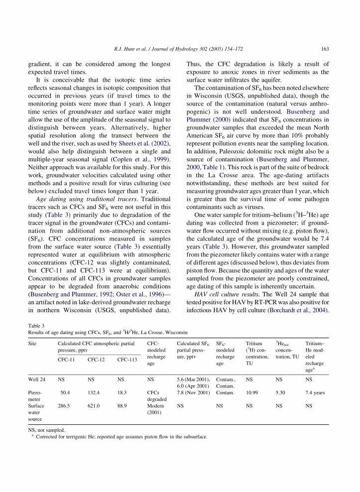
Age dating using traditional tracers. Traditional

tracers such as CFCs and SF6 were not useful in this

study (Table 3) primarily due to degradation of the

tracer signal in the groundwater (CFCs) and contami-

nation from additional non-atmospheric sources

(SF6). CFC concentrations measured in samples

from the surface water source (Table 3) essentially

represented water at equilibrium with atmospheric

concentrations (CFC-12 was slightly contaminated,

but CFC-11 and CFC-113 were at equilibrium).

Concentrations of all CFCs in groundwater samples

appear to be degraded from anaerobic conditions

(Busenberg and Plummer, 1992; Oster et al., 1996)—

an artifact noted in lake-derived groundwater recharge

in northern Wisconsin (USGS, unpublished data).

Table 3

Results of age dating using CFCs, SF6, and 3H/3He, La Crosse, Wisconsi

Site Calculated CFC atmospheric partial

pressure, pptv

CFC-

modeled

recharge

age

Calc

part

ure,CFC-11 CFC-12 CFC-113

Well 24 NS NS NS NS 5.6 (

6.0

Piezo-

meter

50.4 132.4 18.3 CFCs

degraded

7.8

Surface

water

source

286.5 621.0 88.9 Modern

(2001)

NS

NS, not sampled.a Corrected for terrigenic He; reported age assumes piston flow in the s

Thus, the CFC degradation is likely a result of

exposure to anoxic zones in river sediments as the

surface water infiltrates the aquifer.

The contamination of SF6 has been noted elsewhere

in Wisconsin (USGS, unpublished data), though the

source of the contamination (natural versus anthro-

pogenic) is not well understood. Busenberg and

Plummer (2000) indicated that SF6 concentrations in

groundwater samples that exceeded the mean North

American SF6 air curve by more than 10% probably

represent pollution events near the sampling location.

In addition, Paleozoic dolomitic rock might also be a

source of contamination (Busenberg and Plummer,

2000, Table 1). This rock is part of the suite of bedrock

in the La Crosse area. The age-dating artifacts

notwithstanding, these methods are best suited for

measuring groundwater ages greater than 1 year, which

is greater than the survival time of some pathogen

contaminants such as viruses.

One water sample for tritium–helium (3H–3He) age

dating was collected from a piezometer; if ground-

water flow occurred without mixing (e.g. piston flow),

the calculated age of the groundwater would be 7.4

years (Table 3). However, this groundwater sampled

from the piezometer likely contains water with a range

of different ages (discussed below), thus deviates from

piston flow. Because the quantity and ages of the water

sampled from the piezometer are poorly constrained,

age dating of this sample is inherently uncertain.

HAV cell culture results. The Well 24 sample that

tested positive for HAV by RT-PCR was also positive for

infectious HAV by cell culture (Borchardt et al., 2004).

n

ulated SF6

ial press-

pptv

SF6-

modeled

recharge

age

Tritium

(3H) con-

centration,

TU

3Hetrit

concen-

tration, TU

Tritium–

He mod-

eled

recharge

agea

Mar 2001),

(Apr 2001)

Contam.,

Contam.

NS NS NS

(Nov 2001) Contam. 10.99 5.30 7.4 years

NS NS NS NS

ubsurface.


Because enteric viruses in groundwater tend to become

completely inactivated and lose their infectivity within 1

year, this finding suggests that the virus and associated

water had a travel time from the source to the well of less

than 1 year. Unlike other wells in the La Crosse system

near sanitary sewer lines, Well 24 does not have any other

known source of HAV other than the river. Thus, we

conclude that Well 24 does have a component of water

with an associated travel time of less than 1 year.

Age dating using a temperature time series. The

temperature signal of the surface water source can

often be tracked in the groundwater system,

especially where production wells induce infiltration.

Using the simplest analysis, inflection points in a

time series of the temperature in the groundwater

system represent the seasonal changes of infiltrating

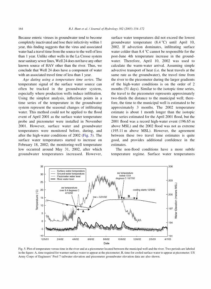
water. This method could not be applied to the flood

event of April 2001 as the surface water temperature

probe and piezometer were installed in November

2001. However, surface water and groundwater

temperatures were monitored before, during, and

after the high-water conditions of 2002 (Fig. 5). The

surface water temperatures started to increase on

February 18, 2002; the monitoring-well temperature

low occurred around May 31, 2002, after which

groundwater temperatures increased. However,

Fig. 5. Plot of temperature versus time in the river and at a piezometer locat

in the figure: A, time required for warmer surface water to appear at the piez

Army Corps of Engineers’ Pool 7 tailwater elevation and piezometer grou

surface water temperatures did not exceed the lowest

groundwater temperature (8.4 8C) until April 10,

2002. If advection dominates, infiltrating surface

water colder than 8.4 8C cannot be responsible for the

post-June 4th temperature increase in the ground-

water. Therefore, April 10, 2002 was used to

calculate the warm-water arrival. Assuming simple

advective transport of heat (i.e. the heat travels at the

same rate as the groundwater), the travel time from

the river to the piezometer during the larger gradients

of the high-water conditions is on the order of 2

months (51 days). Similar to the isotopic time series,

the travel to the piezometer represents approximately

two-thirds the distance to the municipal well; there-

fore, the time to the municipal well is estimated to be

approximately 3 months. The 2002 temperature

estimate is about 1 month longer than the isotopic

time series estimated for the April 2001 flood, but the

2001 flood was a record high-water event (196.65 m

above MSL) and the 2002 flood was not as extreme

(195.11 m above MSL). However, the agreement

between these two travel time estimates is quite

good, and provides additional confidence in the

estimates.

The non-flood conditions have a more subtle

temperature regime. Surface water temperatures

ed between the municipal well and the river. Two periods are labeled

ometer; B, time for cooled surface water to appear at piezometer. US

ndwater elevation data are also shown.


climb relatively steadily until around June 30, 2002,

then fluctuated between 22 and 30 8C until mid-

September (77 days). The signal in the groundwater

system was more muted and did not have a sharp

inflection point at higher temperatures. After the May

31, 2002, low groundwater temperatures climbed until

mid-August, and then remained relatively constant

(around 13.5–13.8 8C) until cooling in December

2002. Similar to the arrival of warmer water discussed

above, the surface water has to be below 13.5 8C

(assuming only advective transport of heat) in order

for cooling at the piezometer to occur; this occurred

on October 7, 2002. Using October 7th, the length of

time for cooler water to arrive at the piezometer is on

the order of 2 months (60 days), and is on the order of

3 months for the municipal well. This yields a non-

flood travel time that is comparable to the 2002 flood

travel time and appreciably shorter than the 2001 non-

flood times calculated by the isotope time series

(about 9 months). This could be a result of a series of

relatively high river stages observed in 2002 that did

not occur in 2001 (Fig. 4). Higher river stages will

increase the hydraulic gradient and advective trans-

port between the river and the piezometer (Fig. 5).

Regardless, the temperature time-series estimates

being on the order of months is consistent with the

isotopic time series.

This temperature analysis uses the following

simplifying assumptions: (1) heat moves through the

subsurface primarily through groundwater advection,

(2) water moves through the aquifer at the same rate

as heat. Although aquifer sediments can also conduct

heat, advection is expected to dominate heat transport

in sediments with high hydraulic conductivity and

appreciable hydraulic gradients such as are found in

high-capacity wellfields. The second assumption is

not as easily addressed; the fact that the range of

temperature fluctuations in the piezometer is smaller

than those in the surface water demonstrates that heat

transport is not fully conservative. However, surface

water heat signals were found over 43 times the

distance observed at Well 24 (albeit, with a smaller

range of temperature fluctuation and longer time lag)

at another location in La Crosse, Wisconsin (USGS,

unpublished data). Thus, heat transport can be

considered sufficiently conservative to investigate

how reasonable a sub-year travel-time estimate is at

the Well 24 site.

Similar to the isotopic time series analysis, the

temperature time series may also reflect seasonality

that occurred in previous years. Unlike stable isotope

ratios, however, temperature is not conserved; thus, the

amplitude of the annual temperature deflection

decreases over time and distance traveled. In some

settings, the signal decline could complicate the use of

longer time-series data or higher spatial resolution data

collected at distances far from the surface water source.

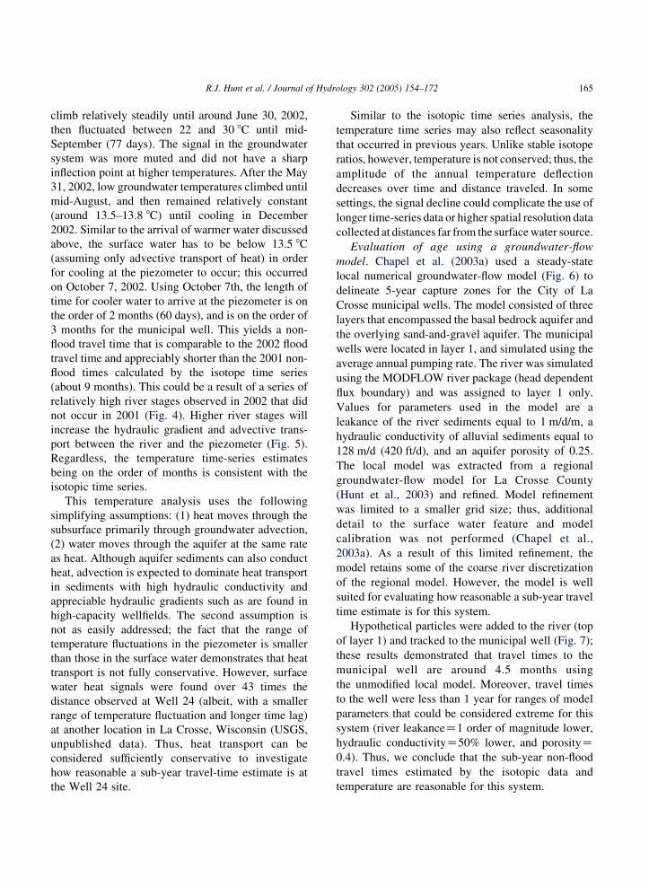
Evaluation of age using a groundwater-flow

model. Chapel et al. (2003a) used a steady-state

local numerical groundwater-flow model (Fig. 6) to

delineate 5-year capture zones for the City of La

Crosse municipal wells. The model consisted of three

layers that encompassed the basal bedrock aquifer and

the overlying sand-and-gravel aquifer. The municipal

wells were located in layer 1, and simulated using the

average annual pumping rate. The river was simulated

using the MODFLOW river package (head dependent

flux boundary) and was assigned to layer 1 only.

Values for parameters used in the model are a

leakance of the river sediments equal to 1 m/d/m, a

hydraulic conductivity of alluvial sediments equal to

128 m/d (420 ft/d), and an aquifer porosity of 0.25.

The local model was extracted from a regional

groundwater-flow model for La Crosse County

(Hunt et al., 2003) and refined. Model refinement

was limited to a smaller grid size; thus, additional

detail to the surface water feature and model

calibration was not performed (Chapel et al.,

2003a). As a result of this limited refinement, the

model retains some of the coarse river discretization

of the regional model. However, the model is well

suited for evaluating how reasonable a sub-year travel

time estimate is for this system.

Hypothetical particles were added to the river (top

of layer 1) and tracked to the municipal well (Fig. 7);

these results demonstrated that travel times to the

municipal well are around 4.5 months using

the unmodified local model. Moreover, travel times

to the well were less than 1 year for ranges of model

parameters that could be considered extreme for this

system (river leakanceZ1 order of magnitude lower,

hydraulic conductivityZ50% lower, and porosityZ0.4). Thus, we conclude that the sub-year non-flood

travel times estimated by the isotopic data and

temperature are reasonable for this system.

Fig. 6. Map showing the groundwater model extent of wellhead protection model of Chapel et al. (2003a). Contour lines represent simulated

groundwater head; contour interval is 0.5 m.


4.3. Implications for water supply investigations

and vulnerability

Surface water can contain many constituents

unsuitable for drinking water such as human

pathogenic viruses, endocrine disrupters, and other

anthropogenic chemicals (Kolpin et al., 2002).

Characterizing the amount of surface water in

a drinking water well facilitates an assessment of

a well’s vulnerability, and is critical for maintaining a

safe water supply. For some microbiological patho-

gens (e.g. viruses), time of travel is paramount to

assessing the susceptibility of the well. Therefore,

methods are needed that are able to discern the

presence of very recent water. Moreover, information

about the associated pathways of transport (overland

versus subsurface) is required in order to develop a

conceptual model of how surface water travels through

the aquifer, as well as to develop a pumping schedule

that can best protect the quality of the water pumped.

Similar to river-wellfield lag times reported by

others (e.g. Maloszewski et al., 1990; Hotzl et al.,

1989; Sheets et al., 2002), four methods used to assess

the travel time from the river to municipal Well 24

are less than 1 year (on the order of 2–9 months).

If piston-flow is assumed for groundwater flow,3H–3He dating estimates approximately 11–12 years

(Table 4). Although the representativeness and repeat-

ability of the 3H–3He age was not evaluated due to

high analytical cost, recent work in the literature

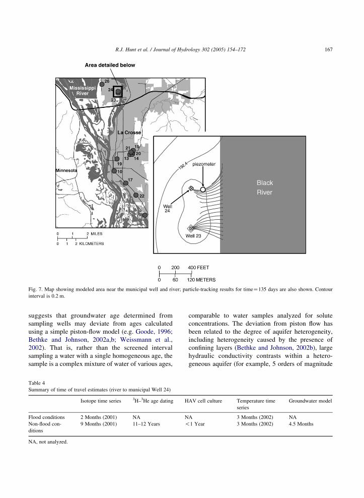
Fig. 7. Map showing modeled area near the municipal well and river; particle-tracking results for timeZ135 days are also shown. Contour

interval is 0.2 m.


suggests that groundwater age determined from

sampling wells may deviate from ages calculated

using a simple piston-flow model (e.g. Goode, 1996;

Bethke and Johnson, 2002a,b; Weissmann et al.,

2002). That is, rather than the screened interval

sampling a water with a single homogeneous age, the

sample is a complex mixture of water of various ages,

Table 4

Summary of time of travel estimates (river to municipal Well 24)

Isotope time series 3H–3He age dating H

Flood conditions 2 Months (2001) NA N

Non-flood con-

ditions

9 Months (2001) 11–12 Years !

NA, not analyzed.

comparable to water samples analyzed for solute

concentrations. The deviation from piston flow has

been related to the degree of aquifer heterogeneity,

including heterogeneity caused by the presence of

confining layers (Bethke and Johnson, 2002b), large

hydraulic conductivity contrasts within a hetero-

geneous aquifer (for example, 5 orders of magnitude

AV cell culture Temperature time

series

Groundwater model

A 3 Months (2002) NA

1 Year 3 Months (2002) 4.5 Months


in Fogg et al., 1999; Weissmann et al., 2002), or large

difference in types of source water (e.g. lake recharge

versus terrestrial recharge reported by Pint et al.,

2003). Of these possible mechanisms for causing

deviation from piston flow, aquifer heterogeneity and

transience appears most likely given the fluvial

sediments of the Mississippi River valley and the

proximity of the river. Additional support for the

shorter travel times calculated by the isotope/tempera-

ture/model approaches is observed in the literature;

Sheets et al. (2002) used a transect of piezometers

between a river and a municipal well to quantify

sub-year travel times in a setting similar to the La

Crosse study site.

If mixing artifacts are the underlying reason for

the conflicting travel-time estimates, why was not the

isotopic time series affected to the same degree as the

tritium–helium sample? The range of d18O variation

in the water sample from the piezometer (with a

sampling point 7 m below the water table) was

smaller than that of the surface water source (Fig.

4), indicating that a mixture of surface water age was

sampled. The effect of the mixing may not have been

as discernible because the old water (having an

appreciably different age) was derived from the same

range of possible surface water isotopic compositions;

thus, the old water would have expected range of

isotopic composition similar to that of the new water.

Time series of stable hydrogen and oxygen isotope

ratios in well-water discharge can be an effective

tool—not only can the amount of surface water in the

well discharge be characterized, information about

travel times can be gained as well. There are, however,

some considerations for successful application. First,

the end-member isotopic compositions and their

variability should be properly characterized. In our

example, we had available the results of a national

database that guide the sampling frequency and total

number of samples for the study. Second, the sampling

plan is most effective if it has both the insight of fixed

interval sampling and the flexibility of event sampling

that can be performed to capture the isotopic

composition of hydrologically important events.

Thirdly, while the flood event was easily seen in the

isotopic composition of the pumping well discharge,

the non-flood time of travel was better observed using a

piezometer installed between the river and the

municipal well. The use of a piezometer simplifies

the interpretation as it is sampling a single flow

direction, unlike the municipal well itself, which is

dominated by radial flow. Finally, the use of isotopic

abundances alone is often non-unique. At the site

discussed here, the stable hydrogen and oxygen

isotopic compositions were complimented with physi-

cal measurements (groundwater level, river stage,

surface water, and groundwater temperature), as well

as a site-specific groundwater-flow model (Chapel et

al., 2003a). While using one method, such as a stable

isotope time series, can give insight into the vulner-

ability of the well, the use of multiple methods is

critical for ensuring this insight is representative of the

system.

5. Conclusions

There are four primary conclusions of this work.

†
The use of the stable hydrogen and oxygen isotopic
composition of water is an effective tool for

describing the influence of surface water on

municipal well supplies. In the City of La Crosse

municipal well network, 7 of the 13 wells are

thought to have appreciable amounts of surface

water contributing to the well water. Multiple

samples over time may be required in order to

identify surface water effects because the isotopic

composition of ambient groundwater is intermedi-

ate to the end members of the surface water

composition. Correct application of this method

will depend on properly characterizing the source

isotopic composition and variability.

†
In addition to identifying the source of water,
analyses of stable hydrogen and oxygen isotope

ratios of water over time can yield insight into the

time of travel from a surface water source to the well.

In the example shown here, surface water required

approximately 2–3 months during flood conditions

and about 9 months during non-flood conditions to

reach the municipal well. The flood events reduce

the travel time by overland inundation (decreasing

the distance) and by increasing the gradient to the

well. While the flood event was recognized by its

isotopic signature in the pumping well discharge,

the non-flood time of travel was better characterized

using a piezometer installed between the river and

the municipal well.


†

Date d18O (‰) d2H (‰)

Surface water (Black

River downstream of

Pool 7 impoundment)

3/12/2001 K9.1 K63.7

4/20/2001 K10.7 K76.5

5/29/2001 K8.7 K63.0

6/25/2001 K8.1 K57.0

7/23/2001 K7.6 K55.5

8/20/2001 K7.1 K51.0

9/24/2001 K7.3 K51.4

10/22/2001 K7.8 K56.3

11/15/2001 K7.9 K58.1

11/16/2001 K7.9 K55.9

11/26/2001 K8.4 K60.5

12/17/2001 K8.6 K59.1

1/30/2002 K8.9 K64.0

1/30/2002 K8.8 K61.4

Traditional age tracers (SF6, CFC) were not useful

at this site because of contamination (SF6) and

degradation (CFC) of the tracers. A tritium–helium

(3H–3He) age in one sample collected from a

piezometer was on the order of 7–8 years if simple

piston flow is assumed, but other methods

estimated travel times of less than 1 year. This

discrepancy suggests that there are age-mass issues

at this site similar to those reported by researchers

in other hydrogeologic settings. Regardless, it is

uncertain if common age dating techniques would

be able to accurately discern travel times on the

order of 1 year or less—the timeframe needed to

assess a well’s vulnerability to pathogens such as

viruses.
1/30/2002 K8.8 K64.1 † 2/16/2002 K9.3 K65.3
2/26/2002 K9.3 K64.6

2/26/2002 K9.2 K65.1

4/9/2002 K9.1 K64.9

4/9/2002 K9.1 K64.9

4/9/2002 K9.5 K65.5

6/5/2002 K8.5 K61.2

8/28/2002 K6.3 K43.2

Well 10 3/12/2001 K8.9 K61.8

4/20/2001 K8.9 K63.6

5/29/2001 K8.9 K61.9

7/23/2001 K8.9 K61.1

8/20/2001 K8.8 K61.4

9/24/2001 K8.8 K60.1

10/22/2001 K8.8 K60.8

11/26/2001 K8.8 K60.2

12/17/2001 K8.8 K60.4

1/30/2002 K8.8 K61.6

2/26/2002 K8.9 K61.7

4/9/2002 K8.9 K62.6

9/4/2002 K8.8 K60.3

Well 13 3/12/2001 K9.0 K59.5

Groundwater temperature variations in a piezo-

meter between the municipal well and the surface

water source yield similar times of travel as those

estimated using isotopic time series. A local

groundwater-flow model also estimated a travel

time of less than 1 year, even for extreme model

parameters. These supporting results increase the

confidence in the time of travel estimated by the

isotopic time series.

As more becomes known about potential sources of

contamination to our groundwater resource, new

techniques will be required to assess accurately a

well’s vulnerability. As shown here, the use of multiple

techniques increased the confidence of our character-

ization. Moreover, with emerging contaminants, such

as viruses, accurate assessments of time of travel, in

addition to water source, are needed to truly protect the

public’s water supply.

11/23/2001 K8.8 K59.6

12/14/2001 K8.8 K60.1

6/5/2002 K8.8 K59.7

Well 14 4/20/2001 K9.0 K61.4

5/29/2001 K9.0 K60.3

6/25/2001 K9.1 K60.8

7/23/2001 K9.0 K60.8

8/20/2001 K9.0 K59.6

9/24/2001 K9.1 K60.0

10/22/2001 K9.0 K60.6

11/26/2001 K9.1 K60.2

12/17/2001 K9.1 K61.3

1/30/2002 K9.0 K62.3

2/26/2002 K9.0 K59.1

6/5/2002 K9.0 K60.8

9/4/2002 K9.0 K61.5

Acknowledgements

The authors would like to thank Tom Berendes

and the City of La Crosse Water Utility for logistical

support throughout the project. The manuscript was

improved by the thorough comments of K. Rozanski

(University of Cracovia, Poland), Rodney Sheets,

David Krabbenhoft, and an anonymous reviewer.

This work was funded by the Wisconsin Department

of Natural Resources and US Geological Survey.

Appendix A. Results of stable isotope sampling in La

Crosse, Wisconsin, USA

Date d18O (‰) d2H (‰)

Well 15 11/26/2001 K8.6 K58.4

12/17/2001 K9.0 K61.1

6/5/2002 K8.6 K58.5

9/5/2002 K8.7 K57.6

Well 17 6/25/2001 K9.0 K61.3

11/25/2001 K8.9 K60.5

12/17/2001 K8.9 K60.7

2/5/2002 K8.9 K61.1

6/5/2002 K8.9 K61.3

9/4/2002 K8.9 K60.0

Well 19 11/26/2001 K8.8 K60.1

12/15/2001 K8.8 K59.7

3/5/2002 K8.8 K58.8

6/5/2002 K8.8 K61.4

9/5/2002 K8.8 K60.0

Well 20 11/26/2001 K8.7 K58.9

12/17/2001 K8.8 K59.5

6/5/2002 K8.8 K59.0

9/5/2002 K8.8 K59.1

Well 21 11/26/2001 K8.6 K59.9

12/17/2001 K8.7 K59.2

2/7/2002 K8.6 K60.4

6/5/2002 K8.6 K59.5

9/5/2002 K8.4 K57.5

Well 22 11/26/2001 K8.9 K60.4

12/15/2001 K8.9 K60.1

2/5/2002 K9.0 K60.6

6/5/2002 K8.9 K60.3

9/5/2002 K8.9 K59.2

Well 23 11/25/2001 K8.6 K60.2

12/16/2001 K8.7 K59.1

2/5/2002 K8.6 K60.9

6/5/2002 K8.7 K60.6

9/4/2002 K8.7 K59.5

Well 24 3/12/2001 K8.4 K58.6

4/20/2001 K8.5 K61.4

5/29/2001 K8.7 K61.8

6/25/2001 K8.9 K60.6

7/23/2001 K8.7 K61.3

8/20/2001 K8.6 K58.9

9/24/2001 K8.5 K59.8

10/22/2001 K8.5 K60.8

11/26/2001 K8.4 K60.2

12/17/2001 K8.5 K59.3

1/30/2002 K8.4 K59.9

2/26/2002 K8.4 K60.4

4/9/2002 K8.5 K61.8

9/4/2002 K8.5 K59.5

Piezometer at Well 24 11/16/2001 K8.6 K61.0

12/17/2001 K8.4 K57.3

1/30/2002 K7.6 K55.8

2/26/2002 K7.5 K54.1

(continued on next page)

Appendix

Date d18O (‰) d2H (‰)

4/9/2002 K7.6 K53.2

6/5/2002 K9.1 K63.1

8/28/2002 K8.8 K60.2

Well 25 3/12/2001 K9.0 K59.1

4/20/2001 K9.0 K60.8

5/29/2001 K9.0 K60.9

6/25/2001 K9.0 K59.7

7/23/2001 K9.0 K60.4

8/20/2001 K8.9 K60.2

9/24/2001 K9.0 K60.2

10/22/2001 K9.0 K61.2

11/26/2001 K9.0 K61.4

12/17/2001 K9.0 K60.3

1/30/2002 K9.0 K61.8

2/26/2002 K9.0 K60.5

6/5/2002 K9.0 K61.1

9/4/2002 K9.0 K60.1

Well 26 11/26/2001 K9.0 K63.6

12/15/2001 K8.9 K61.0

2/6/2002 K8.7 K63.3

9/4/2002 K8.8 K62.0

Appendix


References

Berendes, T.H., 2002. City of La Crosse Water Utility, Written

Communication, October 4, 2002.

Bethke, C.M., Johnson, T.M., 2002a. Paradox of groundwater age.

Geology 30 (2), 107–110.

Bethke, C.M., Johnson, T.M., 2000b. Ground water age. Ground

Water 40 (4), 337–339.

Borchardt, M.A., Haas, N.L., Hunt, R.J., 2004. Vulnerability of

drinking water wells in La Crosse, Wisconsin to enteric virus

contamination from surface water contributions. Applied and

Environmental Microbiology 70, 5937–5946.

Busenberg, E., Plummer, L.N., 1992. Use of chlorofluorocarbons

(CCl3F and CCl2F2) as hydrologic tracers and age-dating

tools—the alluvium and terrace system of Central Oklahoma.

Water Resources Research 28, 2257–2283.

Busenberg, E., Plummer, L.N., 2000. Dating young ground water

with sulfur hexafluoride: natural and anthropogenic sources of

sulfur hexafluoride. Water Resources Research 36, 3011–3030.

Chapel, D.M., Bradbury, K.R., Hunt, R.J., 2003a. Delineation of 5-

year zones of contribution for municipal wells in La Crosse

County 2003. Wisconsin Geological and Natural History Survey

Open File Report 2003-02, Wisconsin.

Chapel, D.M., Bradbury, K.R., Hunt, R.J., Hennings, R.G., 2003b.

Hydrogeology of La Crosse County 2003. Wisconsin Geologi-

cal and Natural History Survey Open File Report 2003-03,

Wisconsin.


Clark, I., Fritz, P., 1997. Environmental Isotopes in Hydrologeol-

ogy. Lewis, Boca Raton, FL. 328 pp.

Coplen, T.B., 1994. Reporting of stable hydrogen, carbon, and

oxygen isotopic abundances. Pure and Applied Chemistry 66,

273–276.

Coplen, T.B., Kendall, C., 2000. Stable isotope and oxygen isotope

ratios for selected sites of the US Geological Survey’s

NASQAN and Benchmark surface-water networks: US Geo-

logical Survey Open-File Report 00-160, 409 pp. http://pubs.

water.usgs.gov/ofr-00-160.

Coplen, T.B., Wildman, J.D., Chen, J., 1991. Improvements in

the gaseous hydrogen–water equilibration technique for

hydrogen isotope ratio analysis. Analytical Chemistry 63,

910–912.

Coplen, T.B., Herczeg, H.L., Barnes, C., 1999. Isotope engineer-

ing—using stable isotopes of the water molecule to solve

practical problems, In: Cook, P., Herczeg, A. (Eds.), Environ-

mental Tracers in Subsurface Hydrology. Kluwer, Boston,

pp. 79–110.

DeBorde, D.C., Woessner, W.W., Lauerman, B., Ball, P.N., 1998.

Virus occurrence and transport in a school septic system and

unconfined aquifer. Ground Water 36, 825–834.

Epstein, S., Mayeda, T., 1953. Variation of O-18 content of

waters from natural sources. Geochim Cosmochimica Acta 4,

213–224.

Evers, S., Lerner, D.N., 1998. How uncertain is our estimate of a

well head protection zone?. Ground Water 36 (1), 49–57.

Fogg, G.E., LaBolle, E.M., Weissmann, G.S., 1999. Ground-

water vulnerability assessment: hydrologic perspective and

example from Salinas Valley, California. In: Assessment

of Non-Point Source Pollution in the Vadose Zone,

American Geophysical Union, Geophysical Monograph

108, pp. 45–61.

Fritz, P., 1981. River water, In: Gat, J.R., Gonfiantini, R.

(Eds.), Stable Isotope Hydrology, Deuterium and Oxygen-18

in the Water Cycle. Technical Report Series no. 210.

International Atomic Energy Agency, Vienna, Austria,

pp. 196–198.

Gat, J.R., 1970. Environmental isotope balance of Lake Tiberias. In:

Isotope Hydrology. International Atomic Energy Agency,

Vienna, pp. 109–127.

Goode, D.J., 1996. Direct simulation of groundwater age. Water

Resources Research 32 (2), 289–296.

Hotzl, H., Reichert, B., Maloszewski, P., Moser, H., Stichler, W.,

1989. Contaminant transport in bank filtration—determining

hydraulic parameters by means of artificial and natural labeling.

In: Contaminant Transport in Groundwater, Balkema, Rotter-

dam, pp. 65–71.

Hunt, R.J., Bullen, T.D., Krabbenhoft, D.P., Kendall, C., 1998.

Using stable isotopes of water and strontium to investigate the

hydrology of a natural and a constructed wetland. Ground Water

36 (3), 434–443.

Hunt, R.J., Steuer, J.J., Mansor, M.T.C., Bullen, T.D., 2001.

Delineating a recharge area for a spring using numerical

modeling, Monte Carlo techniques, and geochemical investi-

gation. Ground Water 39 (5), 702–712.

Hunt, R.J., Saad, D.A., Chapel, D.M., 2003. Numerical Simulation

of Ground Water Flow in La Crosse County, Wisconsin and into

Nearby Pools of the Mississippi River, US Geological Survey

Water-Resources Investigations Report 03-4154 36 pp.

Kendall, C., Coplen, T.B., 2001. Distribution of oxygen-18 and

deuterium in river waters across the United States. Hydrological

Processes 15, 1363–1393.

Kolpin, D.W., Furlong, E.T., Meyer, M.T., Thurman, E.M.,

Zaugg, S.D., Barber, L.B., Buxton, H.T., 2002. Pharmaceu-

ticals, hormones, and other organic wastewater contaminants in

US streams, 1999–2000. A national reconnaissance. Environ-

mental Science and Technology 36 (6), 1202–1211.

Krabbenhoft, D.P., Anderson, M.P., Bowser, C.J., 1990. Estimating

groundwater exchange with lakes, 2. Calibration of a three

dimensional, solute transport model to a stable isotope plume.

Water Resources Research 26 (10), 2455–2462.

Ludin, A., Weppernig, R., Boenisch, G., Schlosser, P., 1997. Mass

spectrometric measurement of helium isotopes and tritium. Lamont-

Doherty Earth Observatory. Technical Report, http://www.ldeo.

columbia.edu/~etg/ms_ms/Ludin_et_al_MS_Paper.html.

Maloszewski, P., Moser, H., Stichler, W., Bertleff, B., Hedin, K.,

1990. Modelling of groundwater pollution by river bank

infiltration using oxygen-18 data. In: Groundwater Monitoring

and Management, Proceedings of the Dresden Symposium,

March 1987. IAHS Publication no. 173, pp. 153–161.

Mazor, E., 1997. Applied Chemical and Isotopic Groundwater

Hydrology, second ed. Marcel Dekker, New York, NY, 413 pp.

McCarthy, K.A., McFarland, W.D., Wilkinson, J.M., White, L.D.,

1992. The dynamic relationship between groundwater and the

Columbia River: using deuterium and oxygen-18 as tracers.

Journal of Hydrology 135, 1–12.

McDonald, M.G., Harbaugh, A.W., 1988. A modular three-

dimensional finite-difference ground-water flow model. US

Geological Survey Techniques of Water-Resources Investi-

gations, Book 6 586 pp (Chapter A1).

Oster, H., Sonntag, C., Munnich, K.O., 1996. Groundwater age

dating with chlorofluorocarbons. Water Resources Research 32,

2989–3001.

Pint, C.D., Hunt, R.J., Anderson, M.P., 2003. Flow path delineation

and ground water age, Allequash Basin, Wisconsin. Ground

Water 41 (7), 895–902.

Pollock, D.W., 1994. User’s Guide for Modpath/Modpath-plot,

Version 3: A Particle Tracking Post-processing Package for

Modflow 1994. The US Geological Survey Finite-difference

Ground-water Flow Model. US Geological Survey Open-File

Report 94-464 (Chapter 6).

Sheets, R.A., Darner, R.A., Whitteberry, B.L., 2002. Lag time of

bank filtration at a well field, Cincinnati, Ohio, USA. Journal of

Hydrology 266, 162–174.

Stichler, W., Moser, H., 1979. An example of exchange between a

lake and groundwater. In: Isotopes in Lake Studes. IAEA,

Vienna, pp. 115–119.

Stichler, W., Maloszewski, P., Moser, H., 1986. Modelling of river

water infiltration using oxygen-18 data. Journal of Hydrology

83, 355–365.

United States Geological Survey, 2003a. SF6 sampling http://

waterusgs.gov/lab/sf6/sampling/.

http://water.usgs.gov/lab/3h3he/sampling/







United States Geological Survey, 2003b. 3H/3He sample collection

http://waterusgs.gov/lab/3h3he/sampling/.

Weissmann, G.S., Zhang, Y., La Bolle, E.M., Fogg, G.E., 2002.

Dispersion of groundwater age in an alluvial aquifer system.

Water Resources Research 38 (10), 10.1029/2001WR000907.

Yates, M.V., Yates, S.R., 1988. Modeling microbial fate in the

subsurface environment. CRC Critical Reviews in Environ-

mental Control 17, 307–344.

Yates, M.V., Gerba, C.P., Kelley, L.M., 1985. Virus persistence

in groundwater. Applied and Environment Microbiology 49,

778–781.

Young, H.L., 1992. Hydrogeology of the Cambrian–Ordovician

Aquifer System in the Northern Midwest, United States 1992.

Geological Survey Professional Paper 1405-B, 99 pp.


Documents

Investigating surface water–well interaction using stable isotope ratios of water