Embed Size (px)
Citation preview
Technical Report Documentation Page
1. Report No.
FHWA/TX-13/0-6657-1
2. Government Accession No.
3. Recipient’s Catalog No.
4. Title and Subtitle
Investigating Regional Dynamic Traffic Assignment Modeling for Improved Bottleneck Analysis: Final Report
5. Report Date
October 2012; Revised March 2013 Published June 2013
6. Performing Organization Code 7. Author(s)
Jennifer C. Duthie, N. Nezamuddin, Natalia Ruiz Juri, Tarun Rambha, Chris Melson, C. Matt Pool, Stephen Boyles, S. Travis Waller, Roshan Kumar
8. Performing Organization Report No.
0-6657-1
9. Performing Organization Name and Address
Center for Transportation Research The University of Texas at Austin 1616 Guadalupe Street, Suite 4.202 Austin, TX 78701
10. Work Unit No. (TRAIS) 11. Contract or Grant No.
0-6657
12. Sponsoring Agency Name and Address
Texas Department of Transportation Research and Technology Implementation Office P.O. Box 5080 Austin, TX 78763-5080
13. Type of Report and Period Covered
Technical Report
September 2010–August 2012
14. Sponsoring Agency Code
15. Supplementary Notes Project performed in cooperation with the Texas Department of Transportation and the Federal Highway Administration.
16. Abstract
This research employed dynamic traffic assignment (DTA) modeling to study the network-wide impact of bottleneck alleviation measures taken by TxDOT on MoPac Expressway in downtown Austin. The measures led to a small improvement in MoPac travel conditions and no major route-switching behaviors were found due to the new geometric reconfiguration on MoPac. The study discussed the benefits and challenges of incorporating DTA into the traditional four-step planning process and provided guidelines to move forward in this direction. A decision-making framework to choose from potential future improvements projects was also developed.
17. Key Words
Dynamic traffic assignment
18. Distribution Statement
No restrictions. This document is available to the public through the National Technical Information Service, Springfield, Virginia 22161; www.ntis.gov.
19. Security Classif. (of report) Unclassified
20. Security Classif. (of this page) Unclassified
21. No. of pages 94
22. Price
Form DOT F 1700.7 (8-72) Reproduction of completed page authorized

Investigating Regional Dynamic Traffic Assignment Modeling for Improved Bottleneck Analysis: Final Report Jennifer C. Duthie N. Nezamuddin Natalia Ruiz Juri Tarun Rambha Chris Melson C. Matt Pool Stephen Boyles S. Travis Waller Roshan Kumar CTR Technical Report: 0-6657-1 Report Date: October 2012; Revised March 2013 Project: 0-6657 Project Title: Investigating Regional Dynamic Traffic Assignment Modeling for Improved
Bottleneck Analysis Sponsoring Agency: Texas Department of Transportation Performing Agency: Center for Transportation Research at The University of Texas at Austin Project performed in cooperation with the Texas Department of Transportation and the Federal Highway Administration.
iv
Center for Transportation Research The University of Texas at Austin 1616 Guadalupe, Suite 4.202 Austin, TX 78701 www.utexas.edu/research/ctr Copyright (c) 2012 Center for Transportation Research The University of Texas at Austin All rights reserved Printed in the United States of America

v
Disclaimers Author's Disclaimer: The contents of this report reflect the views of the authors, who
are responsible for the facts and the accuracy of the data presented herein. The contents do not necessarily reflect the official view or policies of the Federal Highway Administration or the Texas Department of Transportation (TxDOT). This report does not constitute a standard, specification, or regulation.
Patent Disclaimer: There was no invention or discovery conceived or first actually reduced to practice in the course of or under this contract, including any art, method, process, machine manufacture, design or composition of matter, or any new useful improvement thereof, or any variety of plant, which is or may be patentable under the patent laws of the United States of America or any foreign country.
Engineering Disclaimer NOT INTENDED FOR CONSTRUCTION, BIDDING, OR PERMIT PURPOSES.
vi
Acknowledgments The authors would like to express appreciate to the Project Director, Joseph Carrizales,
for providing guidance throughout the project as well as always taking a detailed look at our reports to ensure the best possible quality. We would also like to thank the members of the Project Monitoring Committee, which includes Janie Temple from Transportation Planning and Programming, Dean Wilkerson from the Information Systems Division, and Ed Collins from the Austin District. They also provided much needed guidance during project meetings. Finally, we would like to thank Duncan Stewart for his work as Project Engineer. He dutifully shepherded the project along and we feel fortunate to have had the chance to work closely with him before his retirement. Finally, the authors would like to thank the CTR staff members who helped with document preparation, including Lisa Cramer, Jose Hernandez, Clair LaVaye, and Maureen Kelly.
vii
Table of Contents
Chapter 1. Introduction to Dynamic Traffic Assignment (DTA) ..............................................1 1.1 Why Consider DTA? .............................................................................................................1 1.2 Simulation-Based DTA ..........................................................................................................2 1.3 Review of DTA Software ......................................................................................................5
1.3.1 VISTA (Visual Interactive System for Transportation Algorithms) ..............................6 1.3.2 Dynameq .........................................................................................................................6 1.3.3 DynaMIT .........................................................................................................................7 1.3.4 TRANSIMS ....................................................................................................................7 1.3.5 DYNASMART ...............................................................................................................8 1.3.6 DynusT ............................................................................................................................9
Chapter 2. DTA for Bottleneck Analysis ...................................................................................11 2.1 Bottleneck Identification ......................................................................................................11 2.2 Modeling of Traffic Bottlenecks Using DTA ......................................................................11
Chapter 3. Performance Metrics for Bottleneck Mitigation ....................................................13 3.1 Introduction to Performance Measures ................................................................................13 3.2 Performance Measures for Mitigating Bottlenecks—Review of the Literature ..................13 3.3 Performance Measures for Bottlenecks Derived from DTA ...............................................14 3.4 Volume-Based Performance Measures ................................................................................15
3.4.1 Throughput ....................................................................................................................15 3.4.2 Volume-to-Capacity (V/C) Ratio ..................................................................................15 3.4.3 Route Choice .................................................................................................................16 3.4.4 Density ..........................................................................................................................18
3.5 Travel Time-Based Performance Measures .........................................................................18 3.5.1 Travel Time ...................................................................................................................18 3.5.2 Delay .............................................................................................................................19 3.5.3 Speed .............................................................................................................................19
Chapter 4. Test Bed Bottleneck Site ...........................................................................................21 4.1 Selection of a Test Bed Location .........................................................................................21 4.2 Data Sets ..............................................................................................................................22 4.3 Selection of a DTA Software ...............................................................................................24
Chapter 5. Calibration and Validation of the Base DTA Model .............................................25 5.1 Calibration of DTA Models .................................................................................................25 5.2 Methodology ........................................................................................................................26 5.3 Results ..................................................................................................................................27
5.3.1 Calibration for Ramp Flows ..........................................................................................27 5.3.2 Validation Using Route Travel Times ..........................................................................28
Chapter 6. Evaluating the Impact of MoPac Expressway Lane Reconfigurations on Travel Conditions Using DTA ....................................................................................................31
6.1 Summary of Modeling Goals ...............................................................................................31 6.2 Comparison of Performance Metrics ...................................................................................31
6.2.1 Travel Time ...................................................................................................................31
viii
6.2.2 Vehicular Counts ..........................................................................................................32 6.2.3 Route Choice .................................................................................................................34
6.3 Summary of Findings ...........................................................................................................36
Chapter 7. A Framework to Rank Potential Improvement Projects Using a Simplified Analytical Hierarchy Process ...................................................................................37
7.1 Introduction to Project Ranking ...........................................................................................37 7.2 The Analytical Hierarchy Process .......................................................................................37 7.3 The Developed Decision Making Framework .....................................................................40 7.4 Demonstration of Developed Framework Using MoPac Expressway as a Test Bed ..........40
7.4.1 Defining Focus and Spillback Areas .............................................................................40 7.4.2 Benefit and Cost Estimation .........................................................................................43 7.4.3 Benefit/Cost Analysis and Weighting Process .............................................................45
7.5 Summary of Method ............................................................................................................45
Chapter 8. The Role of DTA in the Transportation Planning Process ...................................47 8.1 Introduction ..........................................................................................................................47 8.2 Review of the Traditional Four-Step Model ........................................................................47 8.3 Integration of DTA and the Four-Step Model at the Regional Level ..................................48 8.4 Integration of DTA and the Four-Step Model at the Sub-Network Level ...........................53
8.4.1 Division of the Mode Choice Model into Finer Time Intervals ...................................53 8.4.2 Introducing Travel Time Unreliability in the Mode Choice Model..............................54
Chapter 9. A Comparison of Dynamic and Static Traffic Assignment Methods ...................57 9.1 Comparison Using the “Before Case” Network ..................................................................58 9.2 Summary of Findings ...........................................................................................................64
Chapter 10. DTA Data and Requirements for Integration with Existing Models .................65 10.1 Introduction ........................................................................................................................65 10.2 Integration ..........................................................................................................................67
10.2.2 Integrating DTA and Macroscopic Models: from TransCAD to VISTA ...................68 10.2.3 Integrating DTA and Microsimulation: from VISTA to VISSIM ..............................71
10.3 Summary of Approach .......................................................................................................74
Chapter 11. Conclusions ..............................................................................................................75
References .....................................................................................................................................77
ix
List of Figures
Figure 1.1: DTA algorithmic procedure ......................................................................................... 4 Figure 1.2: Framework of CTM-based DTA .................................................................................. 5 Figure 3.1: Plot of flow into a roadway link (y-axis) vs. time (x-axis) ........................................ 15 Figure 3.2: Illustration of v/c ratios in downtown Austin ............................................................. 16 Figure 3.3: Example trajectory changes before (blue) and after (yellow) a change to the
network ............................................................................................................................. 16 Figure 3.4: Routes used by all vehicles that traverse a given link ................................................ 17 Figure 3.5: Density (y-axis) vs. time (x-axis) plot ........................................................................ 18 Figure 3.6: Travel time (y-axis) on a link vs. time (x-axis) .......................................................... 18 Figure 4.1: Network for DTA model ............................................................................................ 22 Figure 5.1: Austin regional network (left) and the sub-network (right) ....................................... 26 Figure 5.2: Links directed out (left) and into (right) the network ................................................. 27 Figure 5.3: Routes used for comparison of travel times ............................................................... 29 Figure 6.1: Comparison of MoPac NB travel times (C. Chavez St. exit ramp to Westover
Rd.).................................................................................................................................... 32 Figure 6.2: Comparison of Cesar Chavez/6th Street approach travel times .................................. 32 Figure 6.3: Comparison of 1st/6th Street on-ramp vehicular counts .............................................. 33 Figure 6.4: Comparison of Enfield Road on-ramp vehicular counts ............................................ 33 Figure 6.5: Comparison of travel patterns for origin at 9th and Lavaca and destination at
north MoPac ...................................................................................................................... 34 Figure 6.6: Comparison of travel patterns for origin at CC/5th and destination at north
MoPac ............................................................................................................................... 35 Figure 7.1: Example of hierarchy structure .................................................................................. 39 Figure 7.2: Hierarchy structure for demonstration ....................................................................... 42 Figure 7.3: Focus and spillback areas ........................................................................................... 43 Figure 7.4: Weighted benefit/cost analysis with example calculations ........................................ 45 Figure 8.1: The traditional four-step model .................................................................................. 47 Figure 8.2: Integration of DTA into the four-step model ............................................................. 49 Figure 8.3: Dynamic travel times of Example O-D Pair #1 ......................................................... 50 Figure 8.4: Dynamic travel times of Example O-D Pair #2 ......................................................... 50 Figure 8.5: Dynamic travel times of Example O-D Pair #3 ......................................................... 51 Figure 8.6: Example of the constant proportion assumption ........................................................ 52 Figure 8.7: Integration of DTA and mode choice ......................................................................... 53 Figure 8.8: Dividing simulation period in 15-minute intervals—Example O-D Pair #1 .............. 54 Figure 9.1: Travel time and link volume relationship used in DTA ............................................. 57 Figure 9.2: Travel time and link volume relationship used in STA—The BPR Function ............ 58 Figure 9.3: Fundamental relationship between flow and density ................................................. 58
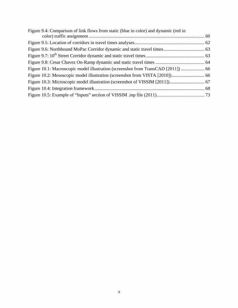
x
Figure 9.4: Comparison of link flows from static (blue in color) and dynamic (red in color) traffic assignment ................................................................................................... 60
Figure 9.5: Location of corridors in travel times analyses............................................................ 62 Figure 9.6: Northbound MoPac Corridor dynamic and static travel times ................................... 63 Figure 9.7: 10th Street Corridor dynamic and static travel times .................................................. 63 Figure 9.8: Cesar Chavez On-Ramp dynamic and static travel times .......................................... 64 Figure 10.1: Macroscopic model illustration (screenshot from TransCAD [2011]) .................... 66 Figure 10.2: Mesoscopic model illustration (screenshot from VISTA [2010]) ............................ 66 Figure 10.3: Microscopic model illustration (screenshot of VISSIM [2011]) .............................. 67 Figure 10.4: Integration framework .............................................................................................. 68 Figure 10.5: Example of “Inputs” section of VISSIM .inp file (2011) ......................................... 73
xi
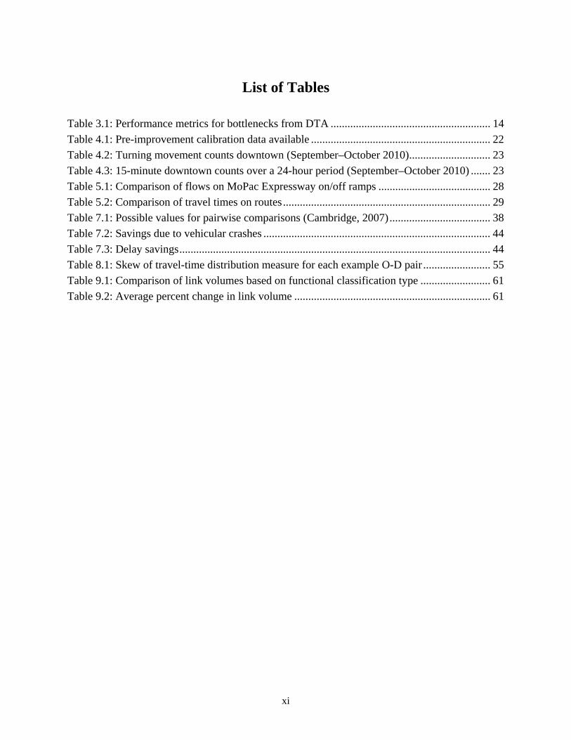
List of Tables
Table 3.1: Performance metrics for bottlenecks from DTA ......................................................... 14 Table 4.1: Pre-improvement calibration data available ................................................................ 22 Table 4.2: Turning movement counts downtown (September–October 2010) ............................. 23 Table 4.3: 15-minute downtown counts over a 24-hour period (September–October 2010) ....... 23 Table 5.1: Comparison of flows on MoPac Expressway on/off ramps ........................................ 28 Table 5.2: Comparison of travel times on routes .......................................................................... 29 Table 7.1: Possible values for pairwise comparisons (Cambridge, 2007) .................................... 38 Table 7.2: Savings due to vehicular crashes ................................................................................. 44 Table 7.3: Delay savings ............................................................................................................... 44 Table 8.1: Skew of travel-time distribution measure for each example O-D pair ........................ 55 Table 9.1: Comparison of link volumes based on functional classification type ......................... 61 Table 9.2: Average percent change in link volume ...................................................................... 61

xii
1
Chapter 1. Introduction to Dynamic Traffic Assignment (DTA)
1.1 Why Consider DTA?
To manage a transportation system or plan for its future, it is necessary to determine the state of the system, current or future. The most fundamental determinant of the state of a roadway network is the vehicular flow pattern on each roadway segment. The pattern forms a basis for subsequent engineering analyses that are used in operational and planning-level decision-making processes. Vehicular flows can be used to study travel times, congestion levels, level of service (LOS), and vehicular emissions. Traditionally, vehicular flows on roadway links are determined by performing a static traffic assignment (STA), which forms the last step in the four-step transportation planning process. The static model of traffic assignment is widely used by planning agencies and traffic management centers. However, the STA model does not account for the time-varying travel conditions of a transportation network. Additionally, STA is unable to model dynamics of traffic flow, such as congestion, queue buildup, bottlenecks, and spillovers in a network.
To fully address complex phenomena such as bottleneck impact, the network-wide evolution of traffic must be represented at a finer resolution than traditional planning tools support. Due to the inability of planning models to fully represent traffic dynamics, operational microscopic models are typically employed to achieve precise time and vehicular movement resolution. However, while microscopic models are capable of capturing these traffic realities, their scope is limited to analyses of corridors or very small sub-areas, as these models lack regional travel behavior models such as equilibrium-based route choice. This limitation demonstrates the need for tools that fill the gap by modeling dynamic traffic at regional scales with expanded and unique functional capabilities. DTA is one such tool that is gaining wide acceptance in the transportation community. DTA has the ability to address realistic transportation planning and operational problems while doing away with the unrealistic assumptions of static approaches (Peeta and Ziliaskopoulos, 2001).
DTA models provide more realistic traffic flow patterns by accounting for changing traffic conditions by time of day. DTA models produce space-time vehicular trajectories consistent with the modeling objective, which is typically one of the following two: minimize total system travel cost or model traffic equilibrium conditions in a network. Vehicular trajectories contain complete information about the state of a transportation system, and form the basis to obtain all other variables characterizing traffic operation in a transportation network.
DTA must be defined as a converged equilibrium solution based on experienced travel costs. Convergence is a critical need for planning applications since a non-converged model cannot be used for project rankings (the model noise/error could easily dominate the impact of scenarios, rendering rankings meaningless). Further, many available DTA tools do not employ experienced travel costs but rather use instantaneous travel costs (Bottom and Chiu, 2011). As noted in the Primer, experienced travel costs are critical and the ideal method of obtaining these metrics is through traffic simulation where rigorous and accepted traffic flow theory is employed, ensuring such realisms as volumes that do not exceed capacity.
For a DTA model to be of value to TxDOT, two additional criteria must be met:
2
1. the ability to model large sub-areas or even regional areas—the area of analysis needs to be large enough to ensure critical traveler behavior, such as changes to route choice and the formation of bottlenecks, is not lost, and
2. the ability to model at a fine time scale—traffic dynamics operate at a very fine time scale (a few seconds) and attempting to aggregate beyond this causes a loss of representation, which negates the benefits of employing DTA.
The following represent the prescribed minimum critical qualities needed by a DTA
model for applications such as system-wide bottleneck analysis:
• Quantifiable convergence based on dynamic user equilibrium
• Regional or large area scope
• Fine time scale (i.e., seconds) used for route choice and simulation
• Mesoscopic simulation approach based on accepted traffic flow theory Put briefly, DTA captures the reality of traffic flows and conditions by accounting for the
time-varying nature of travel times and costs. Each vehicle in the system experiences the travel time/cost that is appropriate given the arrival time of the vehicle on a particular facility. In static assignment, all vehicles experience exactly the same travel time/cost for each facility since travel conditions are assumed to be time invariant. While many operational tools have had these capabilities all along, it must be noted that DTA achieves this correct traffic representation while maintaining accepted travel behavioral models such as regionally equilibrated route choice.
Because of these extensions, DTA models are capable of capturing many realities in the transportation network that static techniques cannot capture, including the following outputs:
1. Vehicle trajectories for every origin-destination (O-D) pair and every time interval.
2. Detailed information characterizing the temporal and spatial dynamics of travel times; traffic counts at specified detector locations; time-varying speed and travel time profiles on links, etc.
3. Congestion indices such as queue lengths; average density and flow; and time-varying density and volume profiles.
Thus, DTA is the ideal tool for modeling bottlenecks at a regional and large sub-area
level. The rest of the chapter is arranged as follows. Section 1.2 describes the procedure for simulation-based DTA. Section 1.3 describes how DTA can be used for bottleneck analysis and a simulation based technique is prescribed for carrying out the proposed plan. A review of available DTA software packages is provided in Section 1.4.
1.2 Simulation-Based DTA
DTA models are divided into analytical and simulation-based models. Since the analytical tools are applicable only for networks consisting of a handful of links and lack traffic flow realism, they are not ready for application to realistic size urban networks. Many analytical models for DTA are often extensions of their static counterparts and are incapable of incorporating rigorous traffic flow models as they model aggregate traffic propagation using
3
link-exit functions. Therefore, these analytical models cannot account for traffic realities like queuing, link spillovers, and shockwave propagation which are common characteristics of congested networks (Waller and Ziliaskopoulos, 2006). Therefore, the present work focuses on the simulation-based DTA models that are able to model realistic networks.
Simulation-based DTA algorithms determine route and link volumes and travel times that satisfy dynamic user equilibrium (DUE) conditions through iterative procedures. Finding a DUE solution (i.e., a set of time-varying link and route volumes and travel costs that satisfy the DUE condition for a given network and time-varying O-D demand pattern) is a non-trivial exercise, because each traveler's best route choice (that is, least experienced travel-cost route) depends on congestion levels throughout the journey. Essentially, the described DTA implementation consists of three critical components: traffic simulation, routing algorithms, and path assignment/optimization. The three steps are described in detail here:
1. Traffic Simulation: This step finds the route travel times from a given set of routes and route choices. There exist a variety of network loading approaches. Simulation-based DTA approaches typically use mesoscopic simulation that simulates changes in traffic flow every ten seconds or less.
2. Routing Algorithms to Update Path Set: Once the network has been loaded, the new shortest paths for every O-D pair are calculated using the new link travel costs. That is, based on the congestion pattern and travel times/costs identified in the network loading step, the routes with the lowest experienced travel-time between every O-D pair, for each departure time period (also called an assignment interval), are found by a time-dependent shortest path (TDSP) algorithm (Ziliaskopoulos and Mahmassani, 1993).
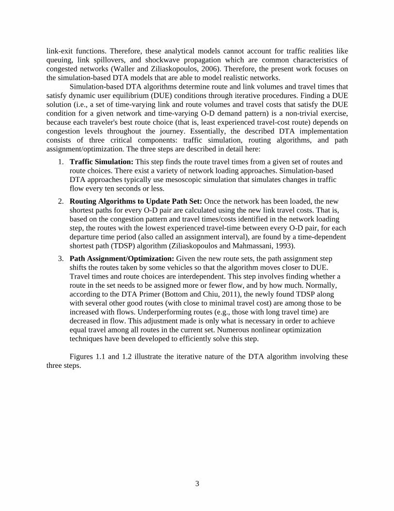
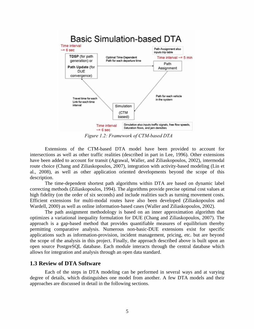
3. Path Assignment/Optimization: Given the new route sets, the path assignment step shifts the routes taken by some vehicles so that the algorithm moves closer to DUE. Travel times and route choices are interdependent. This step involves finding whether a route in the set needs to be assigned more or fewer flow, and by how much. Normally, according to the DTA Primer (Bottom and Chiu, 2011), the newly found TDSP along with several other good routes (with close to minimal travel cost) are among those to be increased with flows. Underperforming routes (e.g., those with long travel time) are decreased in flow. This adjustment made is only what is necessary in order to achieve equal travel among all routes in the current set. Numerous nonlinear optimization techniques have been developed to efficiently solve this step. Figures 1.1 and 1.2 illustrate the iterative nature of the DTA algorithm involving these
three steps.
4
Figure 1.1: DTA algorithmic procedure
These three steps are deployed in a sequential manner till a stopping criterion is met. Figure 1.1 describes the steps involved in such DTA algorithms. Most DTA algorithms use the relative gap, which represents deviation from the ideal DUE condition, as a stopping criterion to measure convergence.
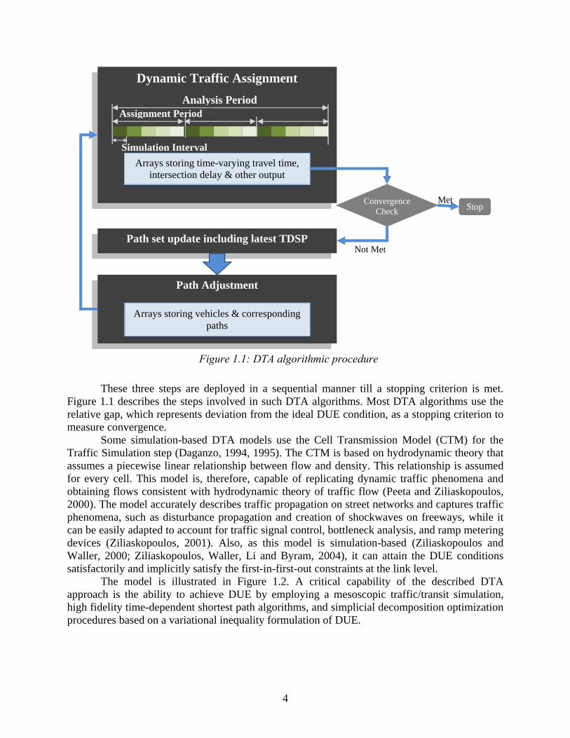
Some simulation-based DTA models use the Cell Transmission Model (CTM) for the Traffic Simulation step (Daganzo, 1994, 1995). The CTM is based on hydrodynamic theory that assumes a piecewise linear relationship between flow and density. This relationship is assumed for every cell. This model is, therefore, capable of replicating dynamic traffic phenomena and obtaining flows consistent with hydrodynamic theory of traffic flow (Peeta and Ziliaskopoulos, 2000). The model accurately describes traffic propagation on street networks and captures traffic phenomena, such as disturbance propagation and creation of shockwaves on freeways, while it can be easily adapted to account for traffic signal control, bottleneck analysis, and ramp metering devices (Ziliaskopoulos, 2001). Also, as this model is simulation-based (Ziliaskopoulos and Waller, 2000; Ziliaskopoulos, Waller, Li and Byram, 2004), it can attain the DUE conditions satisfactorily and implicitly satisfy the first-in-first-out constraints at the link level.
The model is illustrated in Figure 1.2. A critical capability of the described DTA approach is the ability to achieve DUE by employing a mesoscopic traffic/transit simulation, high fidelity time-dependent shortest path algorithms, and simplicial decomposition optimization procedures based on a variational inequality formulation of DUE.
Dynamic Traffic Assignment
Arrays storing time-varying travel time, intersection delay & other output
Path set update including latest TDSP
Path Adjustment
Arrays storing vehicles & corresponding paths
Convergence Check Stop
Assignment Period
Simulation Interval
Analysis Period
Met
Not Met
5
Figure 1.2: Framework of CTM-based DTA
Extensions of the CTM-based DTA model have been provided to account for intersections as well as other traffic realities (described in part in Lee, 1996). Other extensions have been added to account for transit (Agrawal, Waller, and Ziliaskopoulos, 2002), intermodal route choice (Chang and Ziliaskopoulos, 2007), integration with activity-based modeling (Lin et al., 2008), as well as other application oriented developments beyond the scope of this description.
The time-dependent shortest path algorithms within DTA are based on dynamic label correcting methods (Ziliaskopoulos, 1994). The algorithms provide precise optimal cost values at high fidelity (on the order of six seconds) and include realities such as turning movement costs. Efficient extensions for multi-modal routes have also been developed (Ziliaskopoulos and Wardell, 2000) as well as online information-based cases (Waller and Ziliaskopoulos, 2002).
The path assignment methodology is based on an inner approximation algorithm that optimizes a variational inequality formulation for DUE (Chang and Ziliaskopoulos, 2007). The approach is a gap-based method that provides quantifiable measures of equilibrium thereby permitting comparative analysis. Numerous non-basic-DUE extensions exist for specific applications such as information-provision, incident management, pricing, etc. but are beyond the scope of the analysis in this project. Finally, the approach described above is built upon an open source PostgreSQL database. Each module interacts through the central database which allows for integration and analysis through an open data standard.
1.3 Review of DTA Software
Each of the steps in DTA modeling can be performed in several ways and at varying degree of details, which distinguishes one model from another. A few DTA models and their approaches are discussed in detail in the following sections.
6
1.3.1 VISTA (Visual Interactive System for Transportation Algorithms)
VISTA is a DTA software owned by VISTA Transport Group, Inc. (VTG) and operated under a license that allows academics access to the source code. Not only does this access enable a deeper understanding of the algorithms, but it also allows new modeling features and updates to be added to the code as needed. VISTA iterates between two modules: “Path Generation” (PG) and “Dynamic User Equilibrium” (DUE). In the first iteration, PG finds the time-dependent shortest path between each O-D pair at each departure time, assigns all vehicles to their shortest path, and then simulates the vehicle movements to update travel costs. In subsequent iterations of PG, a fixed percentage of vehicles (as opposed to all vehicles) are moved to the shortest path before simulation.
Running an iteration of DUE finds the optimal percentage of vehicles to be shifted from every other path onto the current shortest path. It then simulates these new vehicle trajectories to find new path costs and the new shortest path set. Convergence is measured after both PG and DUE by comparing the travel times across all vehicles with the same origin, destination, and departure time. Convergence is achieved when the travel times are sufficiently close, i.e., the system is in equilibrium.
The simulator is based on the CTM developed by Daganzo (1995). Further refinements were made by Lee (1996) to allow the incorporation of traffic signals and VTG has made many further improvements to, for example, allow for more refined intersection movements, signal optimization, variable message signs, multiple vehicle types including fixed-route transit, and incidents that temporarily reduce capacity.
VISTA can be run from a command line or using the web-based graphical user interface, which includes a geographic information system editor for the purpose of visualizing the network and animating results. More detail on VISTA’s framework can be found in Ziliaskopoulous and Waller (2000). The software has been run successfully on large networks, including the Chicago, Austin, and Dallas/Fort Worth metropolitan planning regions.
1.3.2 Dynameq
Dynameq is a DTA software privately owned by INRO Consultants, Inc. Similar to VISTA, Dynameq is an equilibrium-based model that iterates between finding time-dependent path flows and determining the corresponding path travel times. Vehicles are assigned to paths using the Method of Successive Averages (MSA), which assigns a decreasing fraction of vehicles to the shortest path in subsequent iterations. The fraction is equal to one divided by the current iteration number, so in the first iteration all vehicles are assigned to the shortest path and half of all vehicles are assigned to the shortest path in the second iteration. This differs from the approach taken by VISTA, which is to optimize this fraction in such a way that minimizes the convergence criteria. Vehicles are simulated at a microscopic level to determine path costs. Although Dynameq is an equilibrium-based model (i.e., vehicles do not switch paths en route), lane-changing decisions are made upon entering each new link. Modeling individual lanes has the advantage of explicitly modeling scenarios when certain types of vehicles are restricted from specific lanes (e.g., high occupancy vehicle [HOV] lanes).
To improve computational efficiency and allow for regional-level modeling, Dynameq’s behavioral rules are simplified relative to other microscopic simulators. These simplifications include not allowing vehicles to reconsider their lane choice. Also, the model is updated each time an event occurs, rather than at pre-defined time intervals. Event-based modeling leads to efficiencies, such as when vehicles are waiting at a red light and their position does not need
7
updating at each time interval. The computational effort per link is proportional to the number of vehicles that pass through the link. Dynameq has been successful at modeling medium-sized regions such as Stockholm, Calgary, and San Francisco. More information on Dynameq and its application can be found in Mahut et al. (2004) and Florial et al. (2008).
1.3.3 DynaMIT
DynaMIT (Dynamic Network Assignment for the Management of Information to Travelers) is a DTA model developed at the Massachusetts Institute of Technology. It has an online version that obtains real-time traffic data and predicts network conditions and an offline version mainly used as a planning tool. DyanMIT has two major components—a demand simulator and a supply simulator—that interact with each other to estimate the state of the system.
The demand simulator makes use of historical O-D matrices and generates travelers with certain socio-economic characteristics based on the actual population. Route choice models are then used based on historic travel times to assign a habitual travel behavior for each traveler. In the next step travelers adjust their routes or departure times from their habitual behavior in the presence of network information. This is accomplished by probit or nested logit models using path travel time and cost as trip attributes. The demand is then aggregated and an online calibration model based on an autoregressive process using the Kalman filtering approach adjusts the demands to match real time data. The demand matrices are then disaggregated into individual lists of drivers as in the initial step and are loaded onto the simulator.
The supply simulator captures the behavior of the network using traffic flow models. Links are divided into smaller segments and each segment is divided into a moving part represented by a speed-density relationship and a queuing part. A deterministic queuing model produces the waiting times at queues using the output and acceptance capacities of the segment. Capacities and several other parameters used in the speed-density equations are calibrated both off-line and online. The simulator then updates the speeds and densities by loading the demand on the network in a time-based manner. Vehicles are then advanced to new positions and the process is repeated iteratively.
Most applications of DynaMIT are centered on its predictive abilities and the model was successfully applied to small networks such as Southampton, Lower Westchester County, and Irvine to study various traffic-related problems. More information on DynaMIT can be found in Ben-Akiva et al. (2009).
1.3.4 TRANSIMS
TRANSIMS (Transportation ANalysis and SIMulation System) is an open-source software developed at the Los Alamos National Laboratory to conduct transportation system analysis. It consists of four steps, one of which is an activity-based model to estimate demand, distinguishing it from other assignment models. In the first step, TRANSIMS generates synthetic households and populates them with members using census data. Each member is assigned a vector of socio-demographic characteristics and vehicles are assigned to each household. Based on the land-use data in a given region, the households are placed at appropriate locations in the network.
In the next step, the activities and locations of an individual on a given day are modeled. The start times and end times of different activities are used to determine travel patterns for each individual. Although activity-based models provide disaggregate demands, extensive surveys
8
must be undertaken to estimate such models. This step also models the mode of transport based on survey data. Work locations are obtained using zoning information and gravitational models, while other activities are modeled in such a way that they are close to home or work locations of an individual.
In its third step, TRANSIMS assigns routes to every individual based on his/her activity plans using time-dependent shortest path algorithms. However, very limited dependency between travelers is captured in this stage as the process is interrupted after a few thousand trips and the Bureau of Public Roads functions are used to obtain the link delays. Trips are modeled from activity locations and parking spots, taking into account walking trips for each individual. The process is continued until all trips of every individual are routed.
The last step makes use of a micro-simulator that, working with the route planner, iteratively tries to equilibrate flows. The micro-simulator divides each link into grid cells, each of which is one lane wide and 7.5 meters long. Interactions between vehicles, lane changing, traffic control devices, and queuing are modeled in this step and the average delays for different intervals of time on each link are used to reroute vehicles. A feedback mechanism is used to alter activities in cases where the feasibility of an activity is compromised due to inconsistencies between the arrival time at the destination and the beginning time of the activity. Convergence is tested by comparing the simulated travel times with the best path for each traveler. This path is obtained using an all-or-nothing assignment routing of travelers based on the simulated travel times by day. TRANSIMS has been implemented on large networks such as Dallas and Portland; however, it requires an extensive amount of input data compared to other DTA models. More information about TRANSIMS can be found in Ley (2009).
1.3.5 DYNASMART
DYNASMART (Dynamic Network Assignment-Simulation Model for Advanced Telematics) is a DTA software that employs a simulation-assignment framework to compute transportation network dynamics for different modeling objectives (Mahmassani, 2001). Different modeling objectives use different assignment rules, such as system optimal, user equilibrium, boundedly rational path switching, and current best path assignment.
DYNASMART provides a mesoscopic level of traffic representation, which combines a microscopic level of representation of individual travelers with a macroscopic description of traffic flow. Link movements are calculated using a modified version of Greenshield’s macroscopic speed-density relationship, but vehicular movements are tracked at the level of individual vehicles or groups of vehicles. Delay is computed using node transfers when vehicles transfer between links. The model assumes that O-D demands and departure times are given.
DYNASMART has evolved over more than a decade, extending the first model to include multiple user classes, and various models for information provision and drivers responses to the information provided (Mahmassani and Peeta, 1993, 1995; Mahmassani et al., 1993; Jayakrishnan et al., 1994; Peeta and Mahmassani, 1995). It can model multiple user classes that vary in terms of information availability, information supply strategy, and driver response behavior. DYNASMART can also be used to evaluate the effectiveness of ITS under incident conditions, and for real-time implementation using a rolling horizon framework.
It was tested on the Fort Worth network to evaluate real-time route guidance for incident and non-incident conditions under varying degrees of information supply to different user classes. Additionally, DYNASMART has been tested on the Baltimore and Irvine networks.
9
1.3.6 DynusT
DynusT (Dynamic Urban Systems for Transportation) is an open-source DTA software used for regional operational planning analysis (DynusT, 2011). It uses the Network Explorer for Traffic Analysis (NEXTA) graphical user interface, which provides both data input and simulation animation/data analysis capabilities. DynusT employs a simulation-assignment iterative framework to evaluate long-term impact of altered network conditions, and a one-shot simulation approach for evaluating their short-term impact. It uses the Anisotropic Mesoscopic Simulation (AMS) model for traffic flow propagation, which is a modified version of Greenshield’s model (Chiu et al., 2010). The AMS model defines a speed influencing region (SIR) for each vehicle, and the vehicle’s speed depends upon the average density in its SIR. A vehicle’s SIR consists of a certain specified distance downstream of the vehicle in its lane and the adjacent lanes. In DynustT, the traffic flow model can be specified for each link separately and is chosen from one of two options: single or two regime AMS models.
DynusT defines five user classes (unresponsive, system optimal, user equilibrium, en-route information, and pre-trip information), and their distribution in the traffic stream can be specified as percentages. Its simulation-assignment iterative framework can be run using either the MSA or the gap-function vehicle based assignment algorithm. DynusT provides capability for various modeling applications, such as pricing, work zones, incidents, variable message signs, and ramp metering. It provides an interface to integrate with the VISSIM microscopic simulation model of PTV America. Initial development and testing of the DynusT model were performed on the Phoenix network.

10
11
Chapter 2. DTA for Bottleneck Analysis
2.1 Bottleneck Identification
While DTA represents an emerging transportation modeling tool for numerous potential applications, bottleneck analysis is the quintessential application of DTA for multiple reasons. Two key reasons are that bottleneck analysis requires accurate dynamic traffic representation and that the causes and mitigation for bottlenecks often require a system-wide analysis. The FHWA (2010) recommends the use of mesoscopic tools such as DTA for modeling a series of localized bottlenecks and possibly diversion.
The FHWA defines a bottleneck as a localized constriction of traffic flow—that is, a localized section of highway that experiences reduced speeds and inherent delays due to a recurring operational influence or a nonrecurring impacting event. A bottleneck is different from congestion more generally because bottlenecks usually occur on a section of the parent facility and not along the entire facility. Bottlenecks can be created due to localized incidents that cause the slowing of vehicles. The slowing reduces room to maneuver, which self-perpetuates the shock wave. The problem begins to clear once past the incident, as vehicles begin to accelerate away and maneuvering room downstream of the incident increases (FHWA, 2007). Bottlenecks can also be created at merge points such as intersections or freeway ramps. These types of bottlenecks will be the focus of most of this project since they can be remediated via changes to the roadway geometry.
According to the FHWA, the following conditions typically define the existence of a bottleneck:
• A traffic queue upstream of the bottleneck, wherein speeds are below free-flow conditions present elsewhere on the facility.
• A beginning point for a queue, i.e., a definable point that separates upstream and downstream conditions. The geometry of that point is often coincidently the root cause of the bottleneck.
• Free flow traffic conditions downstream of the bottleneck that have returned to nominal or design conditions.
• Traffic volumes that exceed the capability of the confluence to process traffic. Most bottlenecks can be attributed to the presence of a predictable and recurring cause, as opposed to an amorphous, random event. Therefore, all things being equal, a solution theoretically can be created through correction to the design (FHWA, 2007).
2.2 Modeling of Traffic Bottlenecks Using DTA
Mesoscopic simulation-based DTA models provide vehicle trajectories for every O-D pair for every time-interval. Therefore, it is possible to study queue spillbacks on links and analyze bottlenecks using these models. Bottlenecks can be broadly classified as stationary or moving bottlenecks. Stationary bottlenecks, which are the focus of this research, occur at a specific area due to localized incidents or merging conditions and result in the slowing of vehicles. Some reasons for such bottlenecks include lane drops, lane closures, work zone closures, and minor incidents. One way to evaluate various stationary bottleneck amelioration
12
strategies is through microsimulation, which involves tracking each vehicle in the bottleneck region using car following models (Gentile et al., 2007). These microsimulation models are time-consuming to deploy and evaluate the traffic only in a small region around the bottleneck; network-wide or region-wide impacts cannot be studied using these models. Simulation-based DTA models explicitly account for lanes on the network, and as a result can be used to effectively model a sudden drop in capacity on a particular link. They can also model incidents, queue spillovers due to increased demand at ramps during peak-periods, and various other characteristics that define bottlenecks. Therefore, the effects of stationary bottlenecks can be effectively studied using the proposed DTA models. Moreover, DTA models provide vehicle trajectories for the entire region for the duration of the simulation period. Thus, network-wide impacts of bottlenecks and the various traffic flow parameters that they affect can be thoroughly analyzed. This, in turn, helps in the development and evaluation of amelioration strategies at the network-wide level.
Moving bottlenecks in highway traffic are defined as a situation in which a slow-moving vehicle, be it a truck hauling heavy equipment or an oversized vehicle, or a long convoy, disrupts the continuous flow of the general traffic (Juran et al., 2009). A moving bottleneck is a physical entity that travels through the network, and depending on its position, creates a localized bottleneck in that area. Juran et al. (2009) proposed a mesoscopic simulation-based DTA model that accounts for moving bottlenecks. They proposed a bi-level algorithm to study the moving bottleneck phenomenon. But, their algorithm only accounts for dynamic system optimality and not DUE. The inputs to their model include the traffic network, a time-dependent O-D matrix and one or more bottlenecks with known properties such as the path, physical dimensions and speed. The demands are then distributed in packets which are platoons of vehicles governed by macroscopic traffic flow relationships. At every node a packet is split into smaller packets based on certain splitting ratio.
A key finding in their work is that the impact of a moving bottleneck is a function of average congestion in the network. It was found that in very light and heavy traffic moving bottlenecks had minimal impact on network travel times. The network performance was studied under various scenarios by scaling demands gradually. Additional delays caused due to bottlenecks were found to increase up to a certain point where its effect is greatest. Increasing the demand beyond this point was found to have relatively lesser impact on delays caused due to bottlenecks.
Juran et al. (2009) also explicitly state that relatively few studies examine the behavior of traffic flow around a moving bottleneck on a highway. As of yet no attempt has been made to assess, qualitatively and/or quantitatively, the impact that moving bottlenecks have on the overall performance of a traffic network.
Through this project we will evaluate, using simulation-based DTA models, conditions that cause stationary bottlenecks, their impact on the entire regional transportation network, and strategies to ameliorate these impacts. The research efforts due to this project will result in a comprehensive study of traffic bottleneck phenomena and how they impact the traffic dynamics in a spatio-temporal region-wide network. The team will also develop plans and standards for the potential incorporation of DTA methods into the broader planning process.
13
Chapter 3. Performance Metrics for Bottleneck Mitigation
3.1 Introduction to Performance Measures
Performance measures are quantitative descriptors that allow us to comprehend, manage, and improve various aspects of a transportation network. They help gauge the state of current operational conditions as well as the impacts that changes, such as adding a traffic lane or altering signal timing plans, may have on a transportation network. The careful selection of performance measures is especially critical when analyzing transportation systems since the scenarios being considered for implementation are typically costly.
In the context of transportation networks, performance measures are often characterized by their level of aggregation, i.e., system level, route level, and local level. “System Level” performance measures are aggregated over the region being considered. One example is the average travel time for a vehicle trip in the City of Austin. “Route Level” measures are aggregated over one particular route, usually defined by a corridor. One example is the average delay for a vehicle traveling along IH 35 through downtown Austin. “Local Level” performance measures focus on one link (a network “link” is typically defined as the roadway between two intersections or two ramps) or intersection. Examples include average delay for a particular turning movement at an intersection and the maximum queue on a specified link. Regardless of the scope of the project being evaluated, considering performance measures at all levels is often a good idea since a local improvement to the traffic conditions might not always result in better performance of the system at the network level. In fact, an improvement in one region could worsen the performance of another, resulting in an overall decrease in the system performance. This concern is especially applicable to bottleneck amelioration strategies. For example, even after making improvements to capacities at a bottleneck, the system performance might not improve in cases where the bottleneck shifts to a different location.
As discussed in Chapter 1, DTA models are ideal for studying the system-wide impacts of bottlenecks. Mesoscopic simulation-based DTA models provide vehicle trajectories for every O-D pair for every time-interval. Therefore, these models allow study of queue spillbacks on links and analysis of bottlenecks. DTA models also provide vehicle trajectories for the entire region for the duration of the simulation period. Thus, network-wide impacts of bottlenecks and the various traffic flow parameters that they affect can be thoroughly analyzed. This analysis, in turn, helps in the development and evaluation of amelioration strategies at the network-wide level.
In the following sections we review the literature on performance measures for mitigating bottlenecks, then present some performance measures that can be derived from the outputs of a DTA model and discuss how they can be used to identify bottlenecks and justify strategies proposed to mitigate them.
3.2 Performance Measures for Mitigating Bottlenecks—Review of the Literature
Very few papers in the open literature deal with developing bottleneck-mitigating strategies based on performance measures. Most of the research has concentrated on the evolution of traffic and its behavior at bottlenecks. Gentile et al. (2007), Ben-Akiva et al. (1986), Zhao et al. (2005), Kerner (2002), and Juran et al. (2009) studied traffic bottlenecks within a dynamic framework. Additionally, Ringer (1993) studied three bottlenecks in Texas at the
14
microscopic level, while Berner and Klenov (2003) presented a microscopic theory of how traffic will behave in the presence of highway bottlenecks. The performance measures used by these authors to study traffic behavior will be used in our analysis. Additionally, the performance measures prescribed by the NCHRP Segment 311 report will also be used, but within the context of DTA.
Juran et al. (2009) use the following measures when evaluating moving bottlenecks (e.g., due to a slow moving vehicle) using a DTA model: average trip time, average network speed, percentage additional network travel time (which was observed under varying demands), and the percentage of total trips on certain paths.
Gentile et al. (2007) developed a DTA model that accounts for congestion due to queue spillback. Using this model, they studied traffic behavior in the presence of time-varying bottlenecks. The performance measures that they used to evaluate system and link conditions include link travel times, link exit flow volumes, link inflow volumes, link densities, system travel times, and spillback congestion. A bottleneck is said to propagate when the links with spillback congestion form a loop in the transportation network.
Cassidy and Bertini (1998) studied traffic behavior due to bottlenecks at two highway locations in Toronto, Canada. Some performance measures they used to evaluate the traffic congestion and behavior include average rate of discharge of a queue, evolution of queues over time, total effective capacity due to queues, and flow immediately prior to a queue. They focused on two highway sections and did not study the system-wide effects of these bottlenecks.
In the next section, the outputs pertaining to bottlenecks that are obtained from DTA are described. Most performance measures required for bottleneck analysis, described above, are directly obtained, while others can easily be gleaned by studying some other relevant DTA outputs.
3.3 Performance Measures for Bottlenecks Derived from DTA
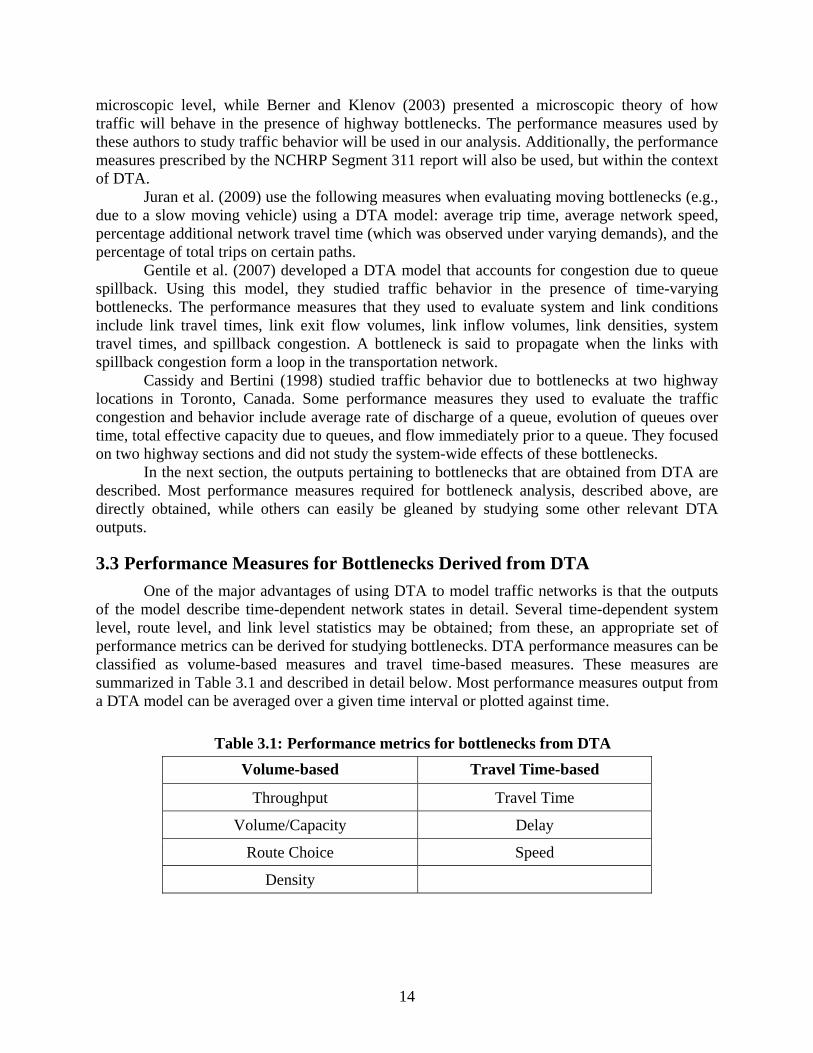
One of the major advantages of using DTA to model traffic networks is that the outputs of the model describe time-dependent network states in detail. Several time-dependent system level, route level, and link level statistics may be obtained; from these, an appropriate set of performance metrics can be derived for studying bottlenecks. DTA performance measures can be classified as volume-based measures and travel time-based measures. These measures are summarized in Table 3.1 and described in detail below. Most performance measures output from a DTA model can be averaged over a given time interval or plotted against time.
Table 3.1: Performance metrics for bottlenecks from DTA
Volume-based Travel Time-based
Throughput Travel Time
Volume/Capacity Delay
Route Choice Speed
Density
15
3.4 Volume-Based Performance Measures
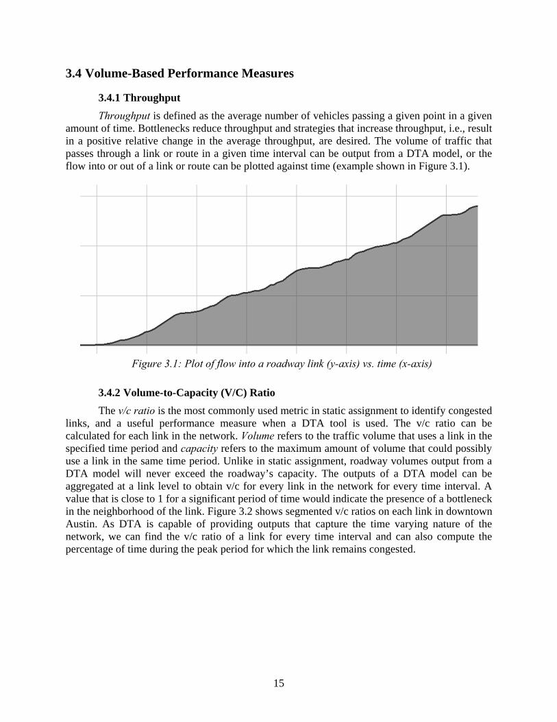
3.4.1 Throughput
Throughput is defined as the average number of vehicles passing a given point in a given amount of time. Bottlenecks reduce throughput and strategies that increase throughput, i.e., result in a positive relative change in the average throughput, are desired. The volume of traffic that passes through a link or route in a given time interval can be output from a DTA model, or the flow into or out of a link or route can be plotted against time (example shown in Figure 3.1).
Figure 3.1: Plot of flow into a roadway link (y-axis) vs. time (x-axis)
3.4.2 Volume-to-Capacity (V/C) Ratio
The v/c ratio is the most commonly used metric in static assignment to identify congested links, and a useful performance measure when a DTA tool is used. The v/c ratio can be calculated for each link in the network. Volume refers to the traffic volume that uses a link in the specified time period and capacity refers to the maximum amount of volume that could possibly use a link in the same time period. Unlike in static assignment, roadway volumes output from a DTA model will never exceed the roadway’s capacity. The outputs of a DTA model can be aggregated at a link level to obtain v/c for every link in the network for every time interval. A value that is close to 1 for a significant period of time would indicate the presence of a bottleneck in the neighborhood of the link. Figure 3.2 shows segmented v/c ratios on each link in downtown Austin. As DTA is capable of providing outputs that capture the time varying nature of the network, we can find the v/c ratio of a link for every time interval and can also compute the percentage of time during the peak period for which the link remains congested.
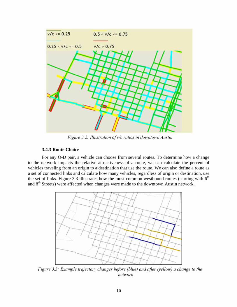
16
Figure 3.2: Illustration of v/c ratios in downtown Austin
3.4.3 Route Choice
For any O-D pair, a vehicle can choose from several routes. To determine how a change to the network impacts the relative attractiveness of a route, we can calculate the percent of vehicles traveling from an origin to a destination that use the route. We can also define a route as a set of connected links and calculate how many vehicles, regardless of origin or destination, use the set of links. Figure 3.3 illustrates how the most common westbound routes (starting with 6th and 8th Streets) were affected when changes were made to the downtown Austin network.
Figure 3.3: Example trajectory changes before (blue) and after (yellow) a change to the
network
17
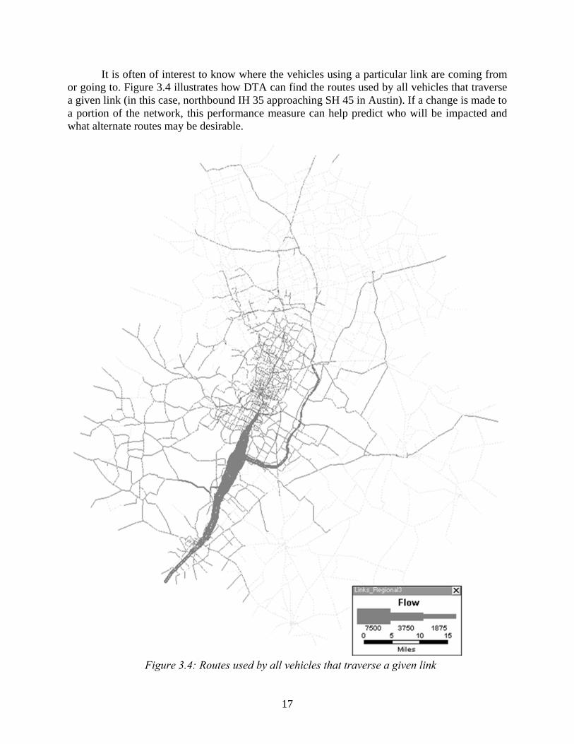
It is often of interest to know where the vehicles using a particular link are coming from or going to. Figure 3.4 illustrates how DTA can find the routes used by all vehicles that traverse a given link (in this case, northbound IH 35 approaching SH 45 in Austin). If a change is made to a portion of the network, this performance measure can help predict who will be impacted and what alternate routes may be desirable.
Figure 3.4: Routes used by all vehicles that traverse a given link
18
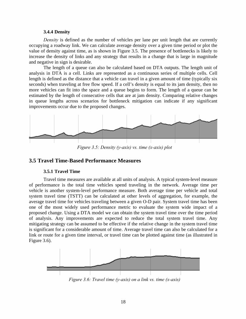
3.4.4 Density
Density is defined as the number of vehicles per lane per unit length that are currently occupying a roadway link. We can calculate average density over a given time period or plot the value of density against time, as is shown in Figure 3.5. The presence of bottlenecks is likely to increase the density of links and any strategy that results in a change that is large in magnitude and negative in sign is desirable.
The length of a queue can also be calculated based on DTA outputs. The length unit of analysis in DTA is a cell. Links are represented as a continuous series of multiple cells. Cell length is defined as the distance that a vehicle can travel in a given amount of time (typically six seconds) when traveling at free flow speed. If a cell’s density is equal to its jam density, then no more vehicles can fit into the space and a queue begins to form. The length of a queue can be estimated by the length of consecutive cells that are at jam density. Comparing relative changes in queue lengths across scenarios for bottleneck mitigation can indicate if any significant improvements occur due to the proposed changes.
Figure 3.5: Density (y-axis) vs. time (x-axis) plot
3.5 Travel Time-Based Performance Measures
3.5.1 Travel Time
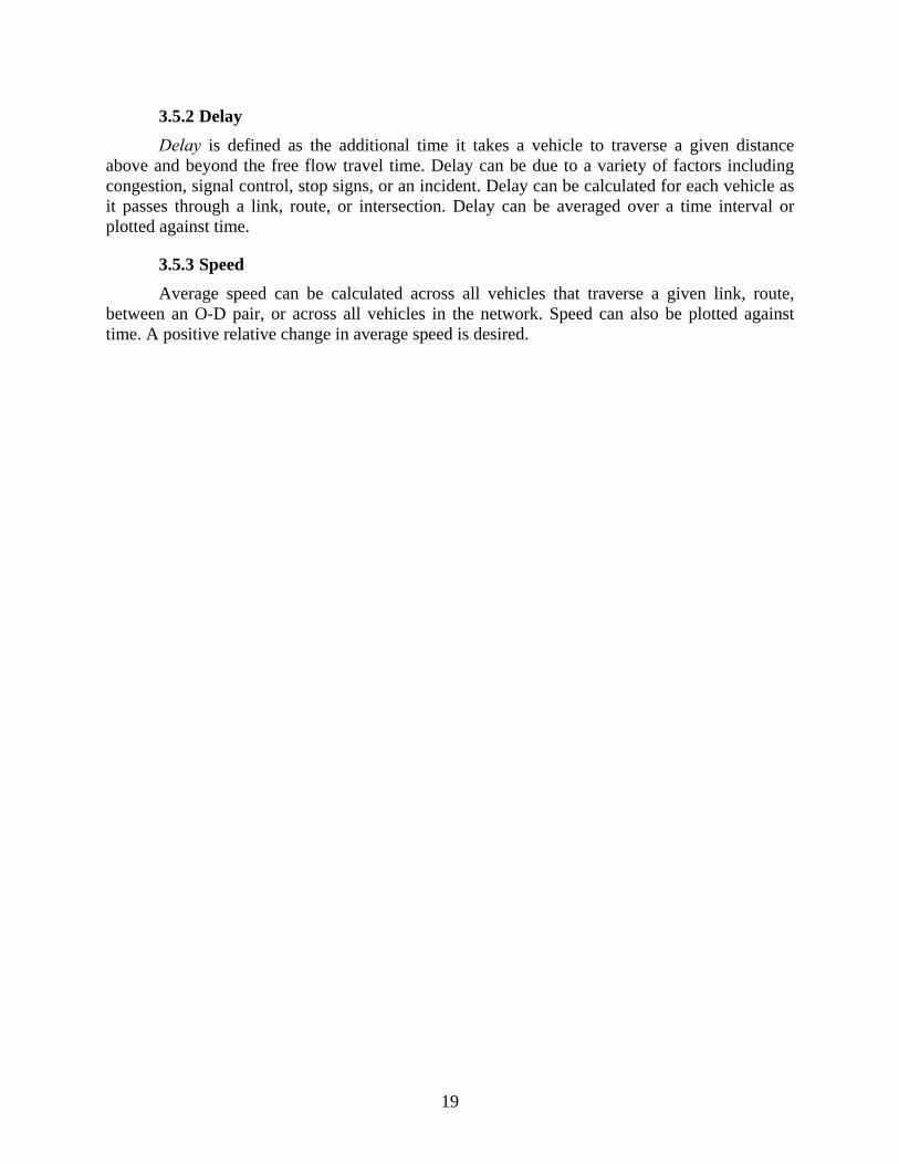
Travel time measures are available at all units of analysis. A typical system-level measure of performance is the total time vehicles spend traveling in the network. Average time per vehicle is another system-level performance measure. Both average time per vehicle and total system travel time (TSTT) can be calculated at other levels of aggregation, for example, the average travel time for vehicles traveling between a given O-D pair. System travel time has been one of the most widely used performance metric to evaluate the system wide impact of a proposed change. Using a DTA model we can obtain the system travel time over the time period of analysis. Any improvements are expected to reduce the total system travel time. Any mitigating strategy can be assumed to be effective if the relative change in the system travel time is significant for a considerable amount of time. Average travel time can also be calculated for a link or route for a given time interval, or travel time can be plotted against time (as illustrated in Figure 3.6).
Figure 3.6: Travel time (y-axis) on a link vs. time (x-axis)
19
3.5.2 Delay
Delay is defined as the additional time it takes a vehicle to traverse a given distance above and beyond the free flow travel time. Delay can be due to a variety of factors including congestion, signal control, stop signs, or an incident. Delay can be calculated for each vehicle as it passes through a link, route, or intersection. Delay can be averaged over a time interval or plotted against time.
3.5.3 Speed
Average speed can be calculated across all vehicles that traverse a given link, route, between an O-D pair, or across all vehicles in the network. Speed can also be plotted against time. A positive relative change in average speed is desired.

20
21
Chapter 4. Test Bed Bottleneck Site
4.1 Selection of a Test Bed Location
Study of the system-wide impact of bottlenecks using DTA involves identification of bottlenecks in a network, and the use of appropriate modeling tools to study the effects of improvements. In this chapter we choose an appropriate DTA model for the analysis of the bottleneck and a test bed location. Analysis using DTA models requires several inputs, such as the network, the test bed location, demand matrices, and various other data discussed in the remainder of this chapter.
Discussions with the Project Monitoring Committee resulted in the decision that the test bed location would be the northbound MoPac Expressway downtown, including the Cesar Chavez Street (aka 1st Street) and 6th Street entrance ramps. In 2010 TxDOT completed a project that resulted in the elimination of a bottleneck in the vicinity of MoPac and 1st/6th Streets. Prior to the project, the number of thru lanes on MoPac was reduced from three to two in the project area. North of the project area, the third lane was reintroduced via an entrance ramp (1st/6th Street) that fed directly into the third lane. To eliminate the bottleneck, it was necessary to reconfigure the mainlanes in a manner that maintained three lanes throughout the corridor. Since the dedicated lane from the entrance ramp was eliminated, traffic entering the expressway must now merge with the mainlane traffic.
The changes included reconfigurations of mainlines, ramps, and acceleration lanes. Two geometric reconfigurations proposed by the TxDOT Austin District were analyzed by the Texas Transportation Institute (TTI), and finally TxDOT adopted Proposal I with changes in the northbound direction only for implementation on the ground (Daganzo, 1994). The geometric changes involved ramp design modifications to allow for three main lanes on MoPac in the northbound direction where only two lanes existed previously. The Enfield Road exit ramp was redesigned such that there is no longer a lane drop from three to two lanes on the mainline. The 1st/6th Street entrance ramp was converted to a merge condition—the ramp was reduced from two lanes to one lane while entering northbound MoPac, and an acceleration lane about 530 feet in length was added. To minimize forced lane-changes ahead of the redesigned single-lane 1st/6th Street entrance ramp, the preceding collector/distributor section on the frontage road was reduced from three to two lanes. These changes were propagated further upstream such that the 1st Street approach reduced from two lanes to one lane before merging with the 6th Street and continuing northbound towards the 1st/6th Street entrance ramp.
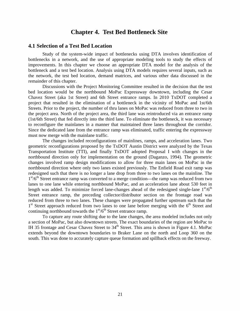
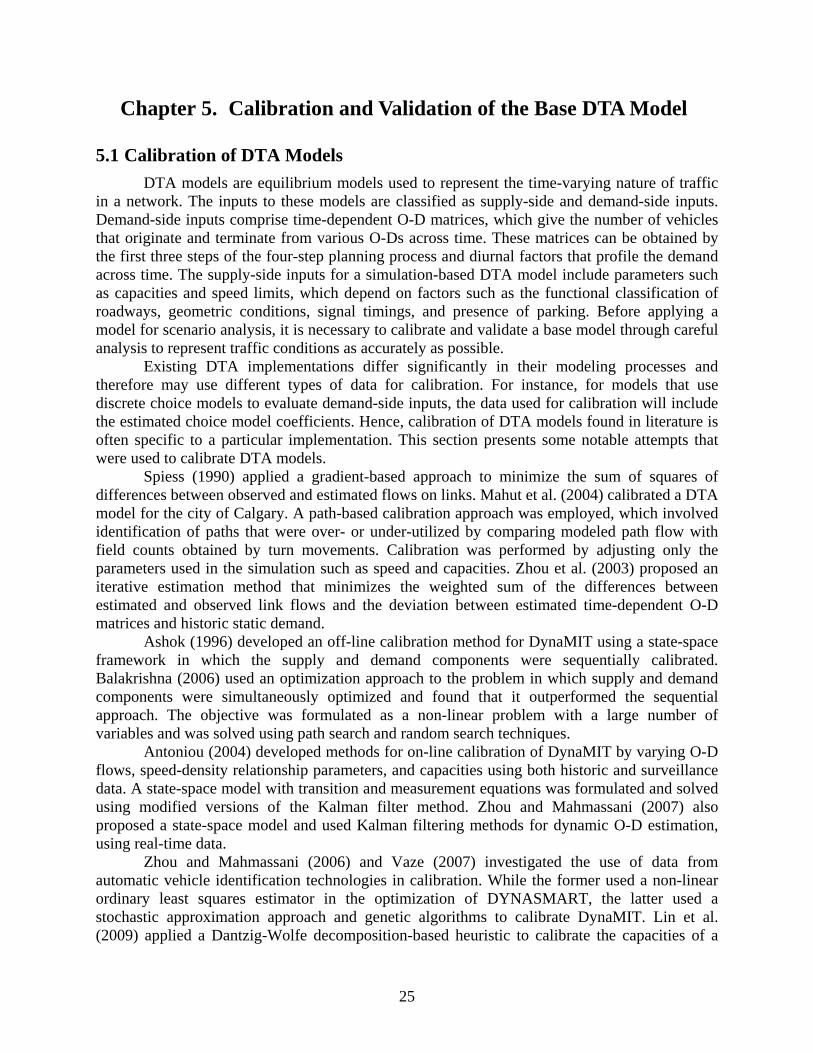
To capture any route shifting due to the lane changes, the area modeled includes not only a section of MoPac, but also downtown streets. The exact boundaries of the region are MoPac to IH 35 frontage and Cesar Chavez Street to 34th Street. This area is shown in Figure 4.1. MoPac extends beyond the downtown boundaries to Braker Lane on the north and Loop 360 on the south. This was done to accurately capture queue formation and spillback effects on the freeway.
22
Figure 4.1: Network for DTA model
4.2 Data Sets
The Capital Area Metropolitan Planning Organization’s (CAMPO) 2010 PM peak demand matrix and the 2010 CAMPO network will be used as the basis for both models. The subnetwork shown in Figure 4.1 is an extraction from the CAMPO regional network, with many refinements made (e.g., adding streets that were missing from the regional model). Adjustments to the demand matrix may be made during calibration. The network used for the post-improvement scenario will also be modified to accurately reflect the improvements.
The research team used the following data for calibrating pre-improvement conditions (see Table 4.1) and post-improvement conditions (see Tables 4.2 and 4.3).
Table 4.1: Pre-improvement calibration data available
Data Type Date Collected
Turning movement counts every 15 minutes at all intersections of MoPac frontage with cross streets (Enfield, Windsor, Westover)
May 2010
Turning movement counts every 15 minutes at southbound MoPac at Lake Austin Blvd.
9/14/10
Speed and travel times between each street crossing MoPac Week of 9/13/10
15-minute counts on MoPac entrance and exit ramps Week of 9/13/10
15-minute counts on MoPac main lanes south of Lake Austin Blvd. (northbound and southbound)
Week of 9/13/10
15-minute downtown cordon counts (IH 35 frontage to Lamar Blvd and Cesar Chavez to approximately 34th St.)
2009
23
Table 4.2: Turning movement counts downtown (September–October 2010)
Turning movement counts
2nd St. at Guadalupe
6th St. at Colorado 9th St. at Lavaca 15th St. at Guadalupe
2nd St. at Lavaca 6th St. at Guadalupe
10th St. at Guadalupe
15th St. at Lavaca
3rd St. at Guadalupe
6th St. at Lavaca 10th St. at Lavaca 15th St. at San Antonio
3rd St. at Lavaca 6th St. at Nueces 11th St. at Guadalupe
Cesar Chavez at Lavaca
4th St. at Guadalupe 7th St. at Guadalupe
11th St. at Lavaca Cesar Chavez at San Antonio
4th St. at Lavaca 7th St. at Lavaca 12th St. at Guadalupe
Congress Ave at MLK
5th St. at Colorado 8th St. at Guadalupe
12th St. at Lavaca Guadalupe at MLK
5th St. at Guadalupe 8th St. at Lavaca 13th St. at Lavaca Lavaca at MLK
5th St. at Lavaca 9th St. at Guadalupe
15th St. at Colorado Nueces at MLK
5th St. at Nueces
Table 4.3: 15-minute downtown counts over a 24-hour period (September–October 2010)
15-minute counts
4th St. at Lavaca 15th St. at Colorado St. Guadalupe at 5th St. Lavaca at 11th St.
4th St. at Guadalupe 15th St. at San Antonio Guadalupe at 6th St. Lavaca at 15th St.
5th St. at Rio Grande
17th St. at Guadalupe Guadalupe at 12th St.
Lavaca at MLK
5th St. at Congress 18th St. at Guadalupe Guadalupe at 16th St.
MLK at Congress
6th St. at Nueces Cesar Chavez at San Antonio
Guadalupe at 20th St.
MLK at Rio Grande
8th St. at Lavaca Cesar Chavez at Congress Lavaca at 5th St. San Antonio at MLK
11th St. at Lavaca Guadalupe at Cesar Chavez Lavaca at 6th St. S. 1st St. Bridge
11th St. at Guadalupe
24
4.3 Selection of a DTA Software
Based on the review of several DTA software and the modeling requirements of this project, VISTA DTA software was chosen for regional DTA modeling for improved bottleneck analysis. This selection was primarily guided by the scope of this study in selecting computationally efficient DTA software: improved bottleneck analysis requires an equilibrium-based DTA model. Travel demand data is given for this study, and the study requires off-line application of the DTA model.
DTA models that estimate travel demand and provide online application features require large amounts of input data and more computational resources. VISTA meets the scope of this project, and its mesoscopic traffic flow model provides an ideal balance between traffic realism and computational efficiency. It employs a traffic flow model based on a CTM, which is consistent with the hydrodynamic model of traffic flow, and models traffic dynamics and shock-wave propagation within a link (Daganzo, 1994). In contrast, most other software models analyze the traffic flows at the link level. Various traffic control systems (stop signs, signal, ramp metering, etc.) can be easily modeled using the cells’ time-dependent parameters. The research team has extensive experience with transportation modeling using VISTA, and the availability of its source code means that new features and updates can be added as needed. Its web-based interface provides flexibility and platform independence. VISTA models can be developed and their results demonstrated on any desktop PC.
25
Chapter 5. Calibration and Validation of the Base DTA Model
5.1 Calibration of DTA Models
DTA models are equilibrium models used to represent the time-varying nature of traffic in a network. The inputs to these models are classified as supply-side and demand-side inputs. Demand-side inputs comprise time-dependent O-D matrices, which give the number of vehicles that originate and terminate from various O-Ds across time. These matrices can be obtained by the first three steps of the four-step planning process and diurnal factors that profile the demand across time. The supply-side inputs for a simulation-based DTA model include parameters such as capacities and speed limits, which depend on factors such as the functional classification of roadways, geometric conditions, signal timings, and presence of parking. Before applying a model for scenario analysis, it is necessary to calibrate and validate a base model through careful analysis to represent traffic conditions as accurately as possible.
Existing DTA implementations differ significantly in their modeling processes and therefore may use different types of data for calibration. For instance, for models that use discrete choice models to evaluate demand-side inputs, the data used for calibration will include the estimated choice model coefficients. Hence, calibration of DTA models found in literature is often specific to a particular implementation. This section presents some notable attempts that were used to calibrate DTA models.
Spiess (1990) applied a gradient-based approach to minimize the sum of squares of differences between observed and estimated flows on links. Mahut et al. (2004) calibrated a DTA model for the city of Calgary. A path-based calibration approach was employed, which involved identification of paths that were over- or under-utilized by comparing modeled path flow with field counts obtained by turn movements. Calibration was performed by adjusting only the parameters used in the simulation such as speed and capacities. Zhou et al. (2003) proposed an iterative estimation method that minimizes the weighted sum of the differences between estimated and observed link flows and the deviation between estimated time-dependent O-D matrices and historic static demand.
Ashok (1996) developed an off-line calibration method for DynaMIT using a state-space framework in which the supply and demand components were sequentially calibrated. Balakrishna (2006) used an optimization approach to the problem in which supply and demand components were simultaneously optimized and found that it outperformed the sequential approach. The objective was formulated as a non-linear problem with a large number of variables and was solved using path search and random search techniques.
Antoniou (2004) developed methods for on-line calibration of DynaMIT by varying O-D flows, speed-density relationship parameters, and capacities using both historic and surveillance data. A state-space model with transition and measurement equations was formulated and solved using modified versions of the Kalman filter method. Zhou and Mahmassani (2007) also proposed a state-space model and used Kalman filtering methods for dynamic O-D estimation, using real-time data.
Zhou and Mahmassani (2006) and Vaze (2007) investigated the use of data from automatic vehicle identification technologies in calibration. While the former used a non-linear ordinary least squares estimator in the optimization of DYNASMART, the latter used a stochastic approximation approach and genetic algorithms to calibrate DynaMIT. Lin et al. (2009) applied a Dantzig-Wolfe decomposition-based heuristic to calibrate the capacities of a
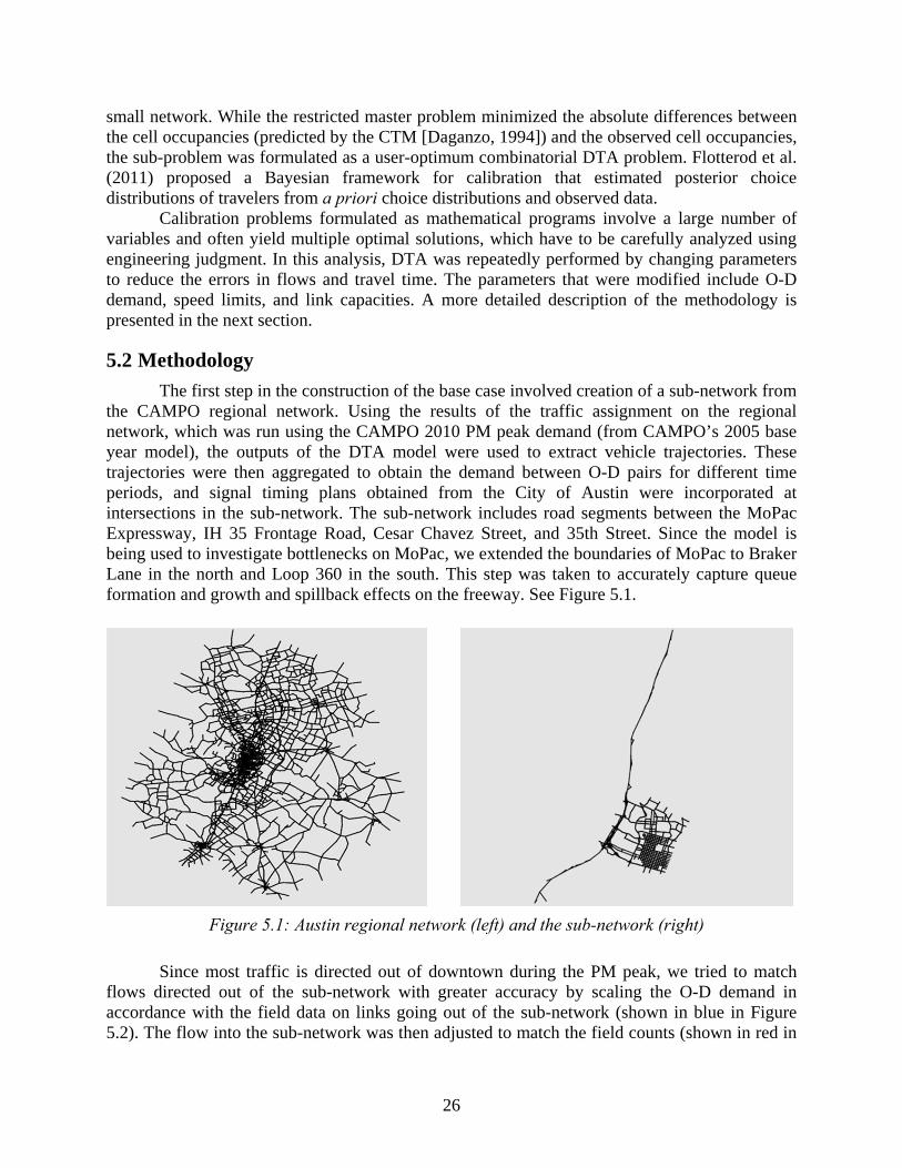
26
small network. While the restricted master problem minimized the absolute differences between the cell occupancies (predicted by the CTM [Daganzo, 1994]) and the observed cell occupancies, the sub-problem was formulated as a user-optimum combinatorial DTA problem. Flotterod et al. (2011) proposed a Bayesian framework for calibration that estimated posterior choice distributions of travelers from a priori choice distributions and observed data.
Calibration problems formulated as mathematical programs involve a large number of variables and often yield multiple optimal solutions, which have to be carefully analyzed using engineering judgment. In this analysis, DTA was repeatedly performed by changing parameters to reduce the errors in flows and travel time. The parameters that were modified include O-D demand, speed limits, and link capacities. A more detailed description of the methodology is presented in the next section.
5.2 Methodology
The first step in the construction of the base case involved creation of a sub-network from the CAMPO regional network. Using the results of the traffic assignment on the regional network, which was run using the CAMPO 2010 PM peak demand (from CAMPO’s 2005 base year model), the outputs of the DTA model were used to extract vehicle trajectories. These trajectories were then aggregated to obtain the demand between O-D pairs for different time periods, and signal timing plans obtained from the City of Austin were incorporated at intersections in the sub-network. The sub-network includes road segments between the MoPac Expressway, IH 35 Frontage Road, Cesar Chavez Street, and 35th Street. Since the model is being used to investigate bottlenecks on MoPac, we extended the boundaries of MoPac to Braker Lane in the north and Loop 360 in the south. This step was taken to accurately capture queue formation and growth and spillback effects on the freeway. See Figure 5.1.
Figure 5.1: Austin regional network (left) and the sub-network (right)
Since most traffic is directed out of downtown during the PM peak, we tried to match flows directed out of the sub-network with greater accuracy by scaling the O-D demand in accordance with the field data on links going out of the sub-network (shown in blue in Figure 5.2). The flow into the sub-network was then adjusted to match the field counts (shown in red in
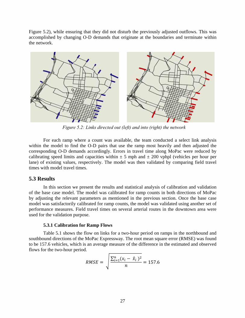
27
Figure 5.2), while ensuring that they did not disturb the previously adjusted outflows. This was accomplished by changing O-D demands that originate at the boundaries and terminate within the network.
Figure 5.2: Links directed out (left) and into (right) the network
For each ramp where a count was available, the team conducted a select link analysis within the model to find the O-D pairs that use the ramp most heavily and then adjusted the corresponding O-D demands accordingly. Errors in travel time along MoPac were reduced by calibrating speed limits and capacities within ± 5 mph and ± 200 vphpl (vehicles per hour per lane) of existing values, respectively. The model was then validated by comparing field travel times with model travel times.
5.3 Results
In this section we present the results and statistical analysis of calibration and validation of the base case model. The model was calibrated for ramp counts in both directions of MoPac by adjusting the relevant parameters as mentioned in the previous section. Once the base case model was satisfactorily calibrated for ramp counts, the model was validated using another set of performance measures. Field travel times on several arterial routes in the downtown area were used for the validation purpose.
5.3.1 Calibration for Ramp Flows
Table 5.1 shows the flow on links for a two-hour period on ramps in the northbound and southbound directions of the MoPac Expressway. The root mean square error (RMSE) was found to be 157.6 vehicles, which is an average measure of the difference in the estimated and observed flows for the two-hour period. = ∑ ( − ) = 157.6
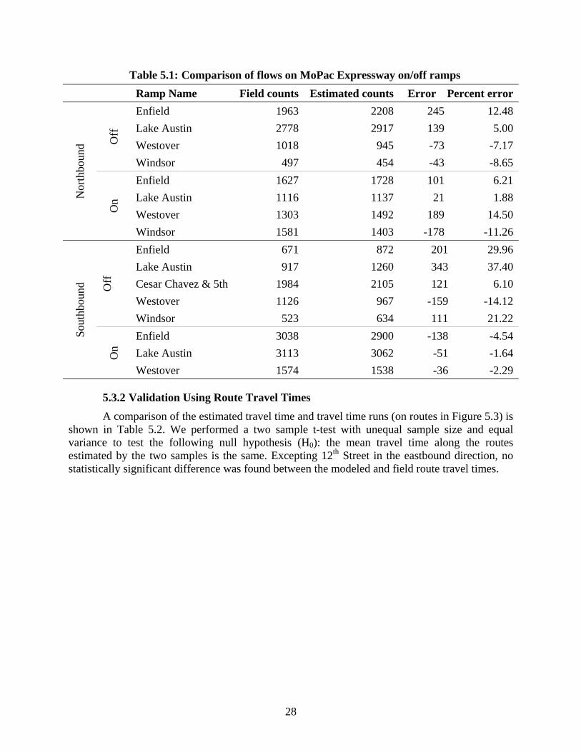
28
Table 5.1: Comparison of flows on MoPac Expressway on/off ramps
Ramp Name Field counts Estimated counts Error Percent errorN
orth
boun
d Off
Enfield 1963 2208 245 12.48
Lake Austin 2778 2917 139 5.00
Westover 1018 945 -73 -7.17
Windsor 497 454 -43 -8.65
On
Enfield 1627 1728 101 6.21
Lake Austin 1116 1137 21 1.88
Westover 1303 1492 189 14.50
Windsor 1581 1403 -178 -11.26
Sou
thbo
und Off
Enfield 671 872 201 29.96
Lake Austin 917 1260 343 37.40
Cesar Chavez & 5th 1984 2105 121 6.10
Westover 1126 967 -159 -14.12
Windsor 523 634 111 21.22
On
Enfield 3038 2900 -138 -4.54
Lake Austin 3113 3062 -51 -1.64
Westover 1574 1538 -36 -2.29
5.3.2 Validation Using Route Travel Times
A comparison of the estimated travel time and travel time runs (on routes in Figure 5.3) is shown in Table 5.2. We performed a two sample t-test with unequal sample size and equal variance to test the following null hypothesis (H0): the mean travel time along the routes estimated by the two samples is the same. Excepting 12th Street in the eastbound direction, no statistically significant difference was found between the modeled and field route travel times.
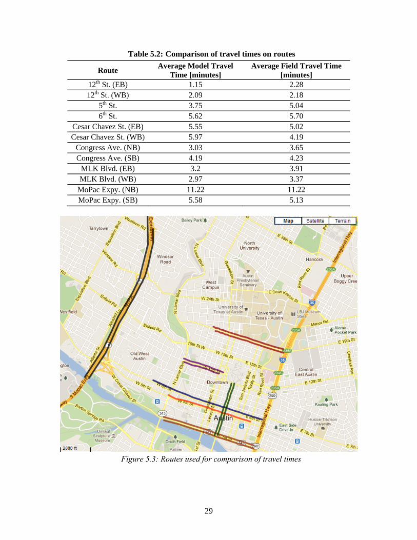
29
Table 5.2: Comparison of travel times on routes
Route Average Model Travel
Time [minutes] Average Field Travel Time
[minutes] 12th St. (EB) 1.15 2.28 12th St. (WB) 2.09 2.18
5th St. 3.75 5.04 6th St. 5.62 5.70
Cesar Chavez St. (EB) 5.55 5.02 Cesar Chavez St. (WB) 5.97 4.19
Congress Ave. (NB) 3.03 3.65 Congress Ave. (SB) 4.19 4.23
MLK Blvd. (EB) 3.2 3.91 MLK Blvd. (WB) 2.97 3.37
MoPac Expy. (NB) 11.22 11.22 MoPac Expy. (SB) 5.58 5.13
Figure 5.3: Routes used for comparison of travel times

30
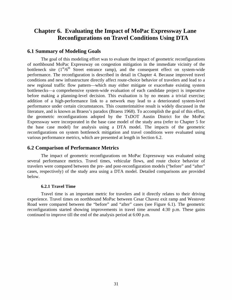
31
Chapter 6. Evaluating the Impact of MoPac Expressway Lane Reconfigurations on Travel Conditions Using DTA
6.1 Summary of Modeling Goals
The goal of this modeling effort was to evaluate the impact of geometric reconfigurations of northbound MoPac Expressway on congestion mitigation in the immediate vicinity of the bottleneck site (1st/6th Street entrance ramp), and the consequent effect on system-wide performance. The reconfiguration is described in detail in Chapter 4. Because improved travel conditions and new infrastructure directly affect route-choice behavior of travelers and lead to a new regional traffic flow pattern—which may either mitigate or exacerbate existing system bottlenecks—a comprehensive system-wide evaluation of each candidate project is imperative before making a planning-level decision. This evaluation is by no means a trivial exercise; addition of a high-performance link to a network may lead to a deteriorated system-level performance under certain circumstances. This counterintuitive result is widely discussed in the literature, and is known as Braess’s paradox (Braess 1968). To accomplish the goal of this effort, the geometric reconfigurations adopted by the TxDOT Austin District for the MoPac Expressway were incorporated in the base case model of the study area (refer to Chapter 5 for the base case model) for analysis using a DTA model. The impacts of the geometric reconfigurations on system bottleneck mitigation and travel conditions were evaluated using various performance metrics, which are presented at length in Section 6.2.
6.2 Comparison of Performance Metrics
The impact of geometric reconfigurations on MoPac Expressway was evaluated using several performance metrics. Travel times, vehicular flows, and route choice behavior of travelers were compared between the pre- and post-reconfiguration models (“before” and “after” cases, respectively) of the study area using a DTA model. Detailed comparisons are provided below.
6.2.1 Travel Time
Travel time is an important metric for travelers and it directly relates to their driving experience. Travel times on northbound MoPac between Cesar Chavez exit ramp and Westover Road were compared between the “before” and “after” cases (see Figure 6.1). The geometric reconfigurations started showing improvements in travel time around 4:30 p.m. These gains continued to improve till the end of the analysis period at 6:00 p.m.
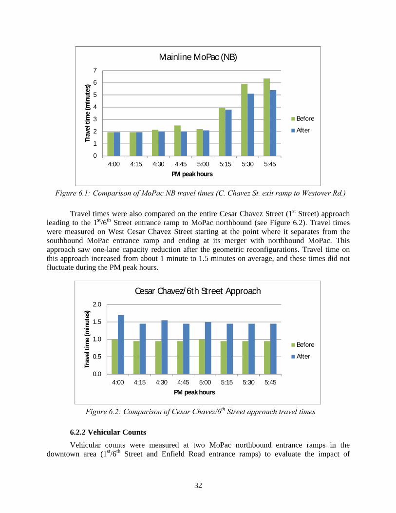
32
Figure 6.1: Comparison of MoPac NB travel times (C. Chavez St. exit ramp to Westover Rd.)
Travel times were also compared on the entire Cesar Chavez Street (1st Street) approach leading to the 1st/6th Street entrance ramp to MoPac northbound (see Figure 6.2). Travel times were measured on West Cesar Chavez Street starting at the point where it separates from the southbound MoPac entrance ramp and ending at its merger with northbound MoPac. This approach saw one-lane capacity reduction after the geometric reconfigurations. Travel time on this approach increased from about 1 minute to 1.5 minutes on average, and these times did not fluctuate during the PM peak hours.
Figure 6.2: Comparison of Cesar Chavez/6th Street approach travel times
6.2.2 Vehicular Counts
Vehicular counts were measured at two MoPac northbound entrance ramps in the downtown area (1st/6th Street and Enfield Road entrance ramps) to evaluate the impact of
0
1
2
3
4
5
6
7
4:00 4:15 4:30 4:45 5:00 5:15 5:30 5:45
Trav
el ti
me
(min
utes
)
PM peak hours
Mainline MoPac (NB)
Before
After
0.0
0.5
1.0
1.5
2.0
4:00 4:15 4:30 4:45 5:00 5:15 5:30 5:45
Trav
el ti
me
(min
utes
)
PM peak hours
Cesar Chavez/6th Street Approach
Before
After
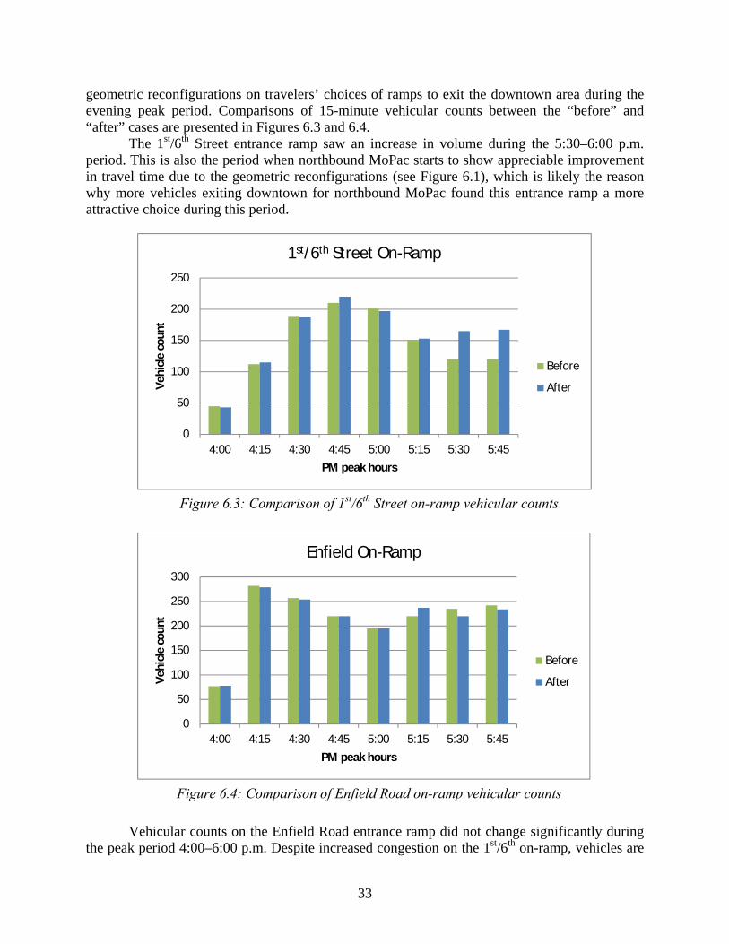
33
geometric reconfigurations on travelers’ choices of ramps to exit the downtown area during the evening peak period. Comparisons of 15-minute vehicular counts between the “before” and “after” cases are presented in Figures 6.3 and 6.4.
The 1st/6th Street entrance ramp saw an increase in volume during the 5:30–6:00 p.m. period. This is also the period when northbound MoPac starts to show appreciable improvement in travel time due to the geometric reconfigurations (see Figure 6.1), which is likely the reason why more vehicles exiting downtown for northbound MoPac found this entrance ramp a more attractive choice during this period.
Figure 6.3: Comparison of 1st/6th Street on-ramp vehicular counts
Figure 6.4: Comparison of Enfield Road on-ramp vehicular counts
Vehicular counts on the Enfield Road entrance ramp did not change significantly during the peak period 4:00–6:00 p.m. Despite increased congestion on the 1st/6th on-ramp, vehicles are
0
50
100
150
200
250
4:00 4:15 4:30 4:45 5:00 5:15 5:30 5:45
Vehi
cle
coun
t
PM peak hours
1st/6th Street On-Ramp
Before
After
0
50
100
150
200
250
300
4:00 4:15 4:30 4:45 5:00 5:15 5:30 5:45
Vehi
cle
coun
t
PM peak hours
Enfield On-Ramp
Before
After
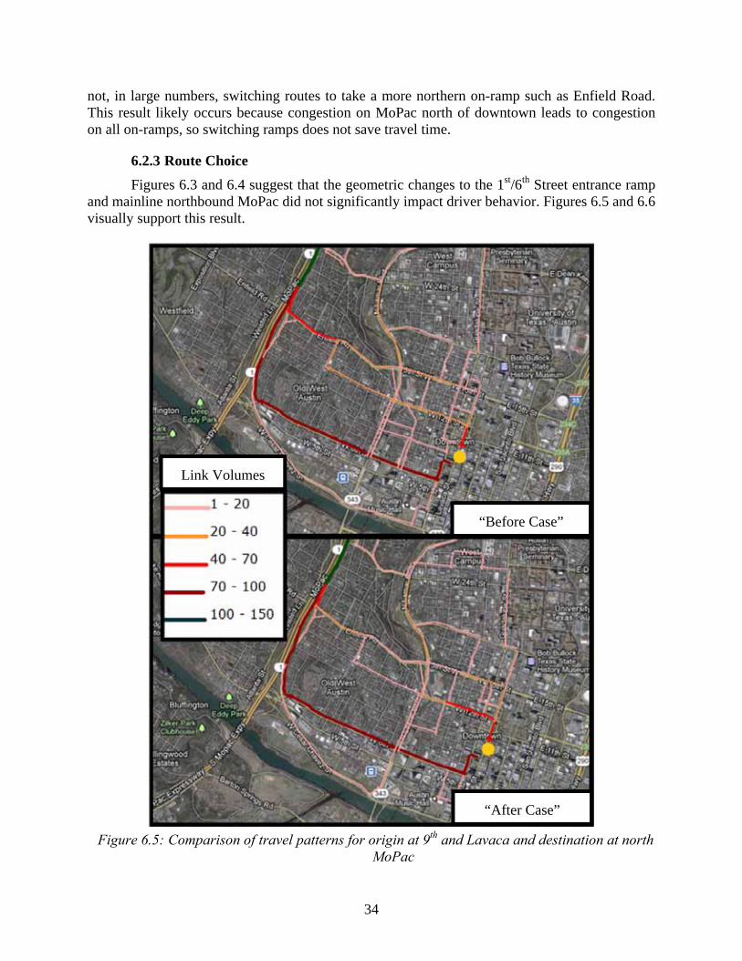
34
not, in large numbers, switching routes to take a more northern on-ramp such as Enfield Road. This result likely occurs because congestion on MoPac north of downtown leads to congestion on all on-ramps, so switching ramps does not save travel time.
6.2.3 Route Choice
Figures 6.3 and 6.4 suggest that the geometric changes to the 1st/6th Street entrance ramp and mainline northbound MoPac did not significantly impact driver behavior. Figures 6.5 and 6.6 visually support this result.
Figure 6.5: Comparison of travel patterns for origin at 9th and Lavaca and destination at north
MoPac
Link Volumes
“Before Case”
“After Case”
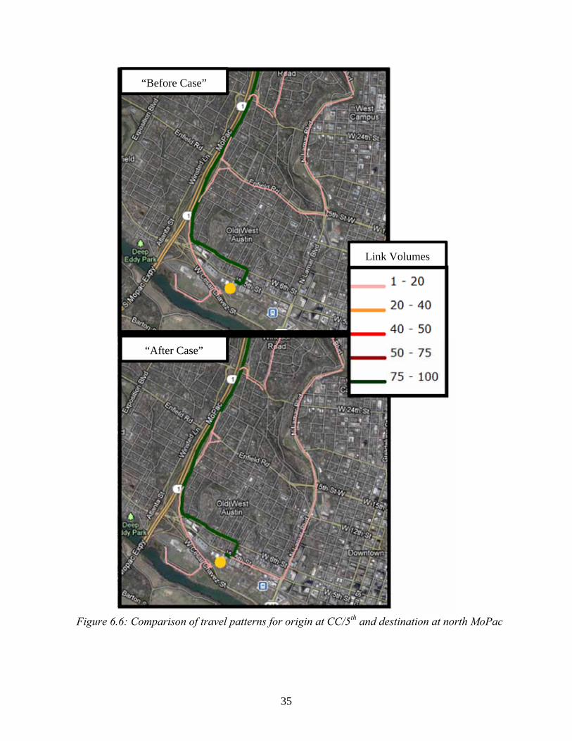
35
Figure 6.6: Comparison of travel patterns for origin at CC/5th and destination at north MoPac
“After Case”
“Before Case”
Link Volumes
36
As shown in Figures 6.5 and 6.6, the travel patterns in the “before” and the “after” cases are essentially the same. Drivers did not switch their route away from the 1st/6th Street ramp and onto other ramps, such as the Enfield Road entrance ramp.
6.3 Summary of Findings
The geometric reconfigurations on northbound MoPac Expressway resulted in a small improvement in travel time during the evening peak period. The 1st/6th Street entrance ramp to northbound MoPac saw a small increase in volume towards the end of the peak period, but there were no major shifts in travel patterns of the commuters leaving downtown in the evening. Overall, no major route switching behavior was observed in the network.
37
Chapter 7. A Framework to Rank Potential Improvement Projects Using a Simplified Analytical Hierarchy Process
7.1 Introduction to Project Ranking
Transportation planning and project evaluation techniques have been a subject of extensive study for many years and provide an essential instrument to transportation agencies across the country. Many agencies have developed their own project evaluation framework; other research entities have created frameworks and guidelines as well. One of the most used planning guidelines in public transportation is A Guidebook for Performance-Based Transportation Planning developed by the National Cooperative Highway Research Program (NCHRP) (Cambridge Systematics, Inc.). Motivation for performance-based planning has increased in the last 15 years and comes from a variety of sources: ISTEA and subsequent federal legislation, heightened concern over the effective use of scarce funding, social and equity concerns, and environmental regulations. Performance-based planning requires agencies to (1) develop goals, (2) subdivide those broad goals into more specific, and more tangible, objectives, and (3) evaluate projects and alternatives based on performance measures, which quantify how well each project satisfies a given objective—and therefore, the goals of the agency. Standard practice is to convert all performance measures into a single unit: capital. Then a cost-benefit ratio is calculated, and the projects are ranked accordingly. The decision-making framework developed for this project combines elements from the typical cost-benefit analysis and the Analytical Hierarchy Process described below.
7.2 The Analytical Hierarchy Process
The Analytical Hierarchy Process (AHP) is primarily used for complicated decision-making that involves both qualitative and quantitative elements. It requires significant user input, having the user or multiple users determine which aspects of the project are most important in completing a set goal or objective. For evaluating transportation alternatives, the qualitative portion consists of users determining the weights of each objective or criterion based on their knowledge and background (i.e., how important the subcategory is to accomplishing the predefined goal). The quantitative aspect involves measuring how well each alternative accomplishes an objective (using measures such as total system travel time, average speed, density, etc.).
As the name suggests, AHP entails the creation of a hierarchy. This hierarchy consists of the main goals at the top tier, potentially more objectives/goals underneath that, then performance measures to estimate the objectives, and finally the alternatives. Figure 7.1 on the next page shows an example hierarchy structure. It is based on TxDOT’s main goals and is the initial hierarchy structure employed for this project.
In a true AHP, evaluators would need to conduct pairwise comparisons of every element in levels (1) and (2). For example, using the structure in Figure 7.1, evaluators would compare the importance of each goal in Tier 2 with every other goal in Tier 2 using the weightings illustrated in Table 7.1. For example, if the main purpose of the project involved preventing bottleneck formation on MoPac, the pairing value of Promote Congestion Relief versus Enhance Safety could be “9” (indicating extreme importance) for the focus area. This comparison could
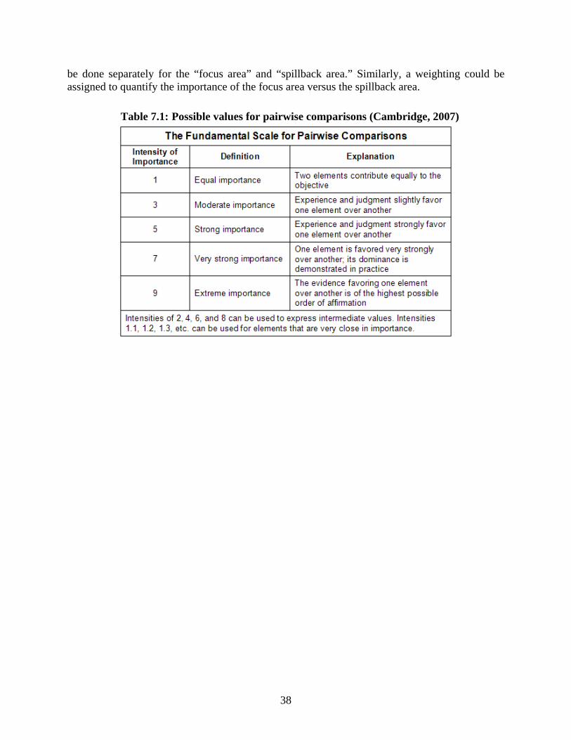
38
be done separately for the “focus area” and “spillback area.” Similarly, a weighting could be assigned to quantify the importance of the focus area versus the spillback area.
Table 7.1: Possible values for pairwise comparisons (Cambridge, 2007)
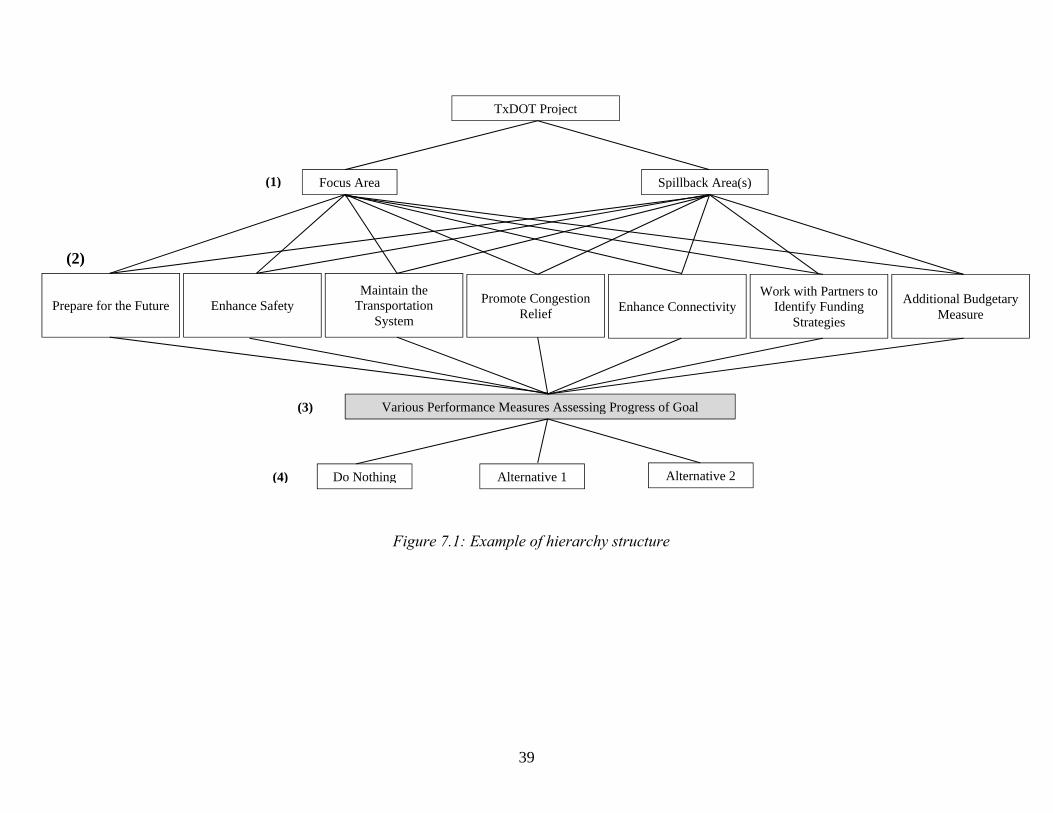
39
Figure 7.1: Example of hierarchy structure
TxDOT Project
Focus Area Spillback Area(s)
Prepare for the Future Enhance Safety Maintain the
Transportation System
Promote Congestion Relief Enhance Connectivity
Work with Partners to Identify Funding
Strategies
Additional Budgetary Measure
Various Performance Measures Assessing Progress of Goal
Do Nothing Alternative 1 Alternative 2
(1)
(3)
(4)
(2)
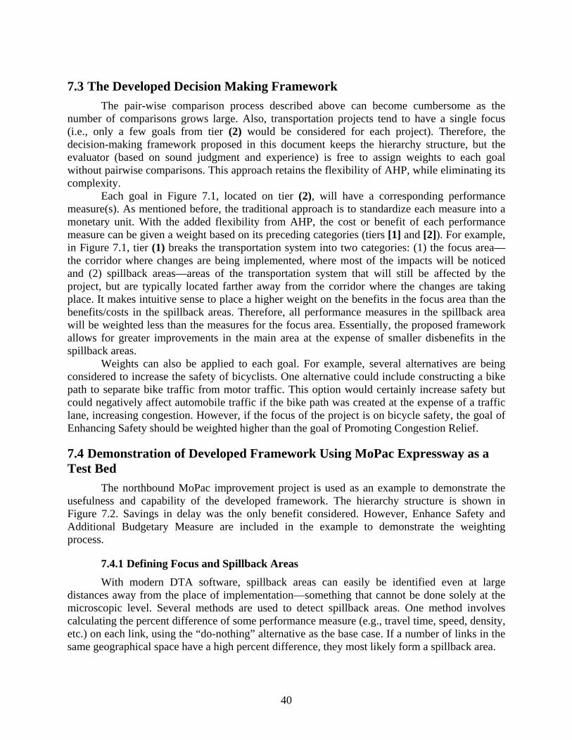
40
7.3 The Developed Decision Making Framework
The pair-wise comparison process described above can become cumbersome as the number of comparisons grows large. Also, transportation projects tend to have a single focus (i.e., only a few goals from tier (2) would be considered for each project). Therefore, the decision-making framework proposed in this document keeps the hierarchy structure, but the evaluator (based on sound judgment and experience) is free to assign weights to each goal without pairwise comparisons. This approach retains the flexibility of AHP, while eliminating its complexity.
Each goal in Figure 7.1, located on tier (2), will have a corresponding performance measure(s). As mentioned before, the traditional approach is to standardize each measure into a monetary unit. With the added flexibility from AHP, the cost or benefit of each performance measure can be given a weight based on its preceding categories (tiers [1] and [2]). For example, in Figure 7.1, tier (1) breaks the transportation system into two categories: (1) the focus area—the corridor where changes are being implemented, where most of the impacts will be noticed and (2) spillback areas—areas of the transportation system that will still be affected by the project, but are typically located farther away from the corridor where the changes are taking place. It makes intuitive sense to place a higher weight on the benefits in the focus area than the benefits/costs in the spillback areas. Therefore, all performance measures in the spillback area will be weighted less than the measures for the focus area. Essentially, the proposed framework allows for greater improvements in the main area at the expense of smaller disbenefits in the spillback areas.
Weights can also be applied to each goal. For example, several alternatives are being considered to increase the safety of bicyclists. One alternative could include constructing a bike path to separate bike traffic from motor traffic. This option would certainly increase safety but could negatively affect automobile traffic if the bike path was created at the expense of a traffic lane, increasing congestion. However, if the focus of the project is on bicycle safety, the goal of Enhancing Safety should be weighted higher than the goal of Promoting Congestion Relief.
7.4 Demonstration of Developed Framework Using MoPac Expressway as a Test Bed
The northbound MoPac improvement project is used as an example to demonstrate the usefulness and capability of the developed framework. The hierarchy structure is shown in Figure 7.2. Savings in delay was the only benefit considered. However, Enhance Safety and Additional Budgetary Measure are included in the example to demonstrate the weighting process.
7.4.1 Defining Focus and Spillback Areas
With modern DTA software, spillback areas can easily be identified even at large distances away from the place of implementation—something that cannot be done solely at the microscopic level. Several methods are used to detect spillback areas. One method involves calculating the percent difference of some performance measure (e.g., travel time, speed, density, etc.) on each link, using the “do-nothing” alternative as the base case. If a number of links in the same geographical space have a high percent difference, they most likely form a spillback area.

41
For the MoPac improvement project, the focus and spillback areas were defined before any detailed analysis was conducted. The focus area contains the northbound mainline of MoPac near the downtown area. The spillback areas include the Cesar Chavez/6th Street entrance ramp and the Enfield Road on-ramp. The secondary spillback area encompasses the downtown region between 6th Street and the bridges over Lady Bird Lake. Based on our model results (see Chapter 5), there was minimal route-changing behavior—thus limiting the effects of the project to the focus and spillback areas only (i.e., few if any changes occurred between the “before case” and “after case” in the secondary spillback area). Therefore, the secondary spillback area will not be included in the project selection process demonstration. The focus area (highlighted in purple), the spillback area (highlighted in green), and the secondary spillback areas are shown in Figure 7.3.
The authors believe the limited variation in travel patterns was caused by a large bottleneck that formed far north of the focus area. During the modeled time period (4:00–6:00 p.m.), the bottleneck steadily migrated backward, causing the majority of northbound MoPac to become congested. Therefore, switching routes would not save the user travel time—no matter what on-ramp is being used, the traveler would still experience the same congestion on MoPac.
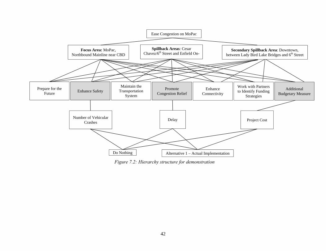
42
Figure 7.2: Hierarchy structure for demonstration
Ease Congestion on MoPac
Focus Area: MoPac, Northbound Mainline near CBD
Spillback Areas: Cesar Chavez/6th Street and Enfield On-
Prepare for the Future
Enhance Safety Maintain the
Transportation System
Promote Congestion Relief
Enhance Connectivity
Work with Partners to Identify Funding
Strategies
Additional Budgetary Measure
Number of Vehicular Crashes
Do Nothing Alternative 1 – Actual Implementation
Delay Project Cost
Secondary Spillback Area: Downtown, between Lady Bird Lake Bridges and 6th Street
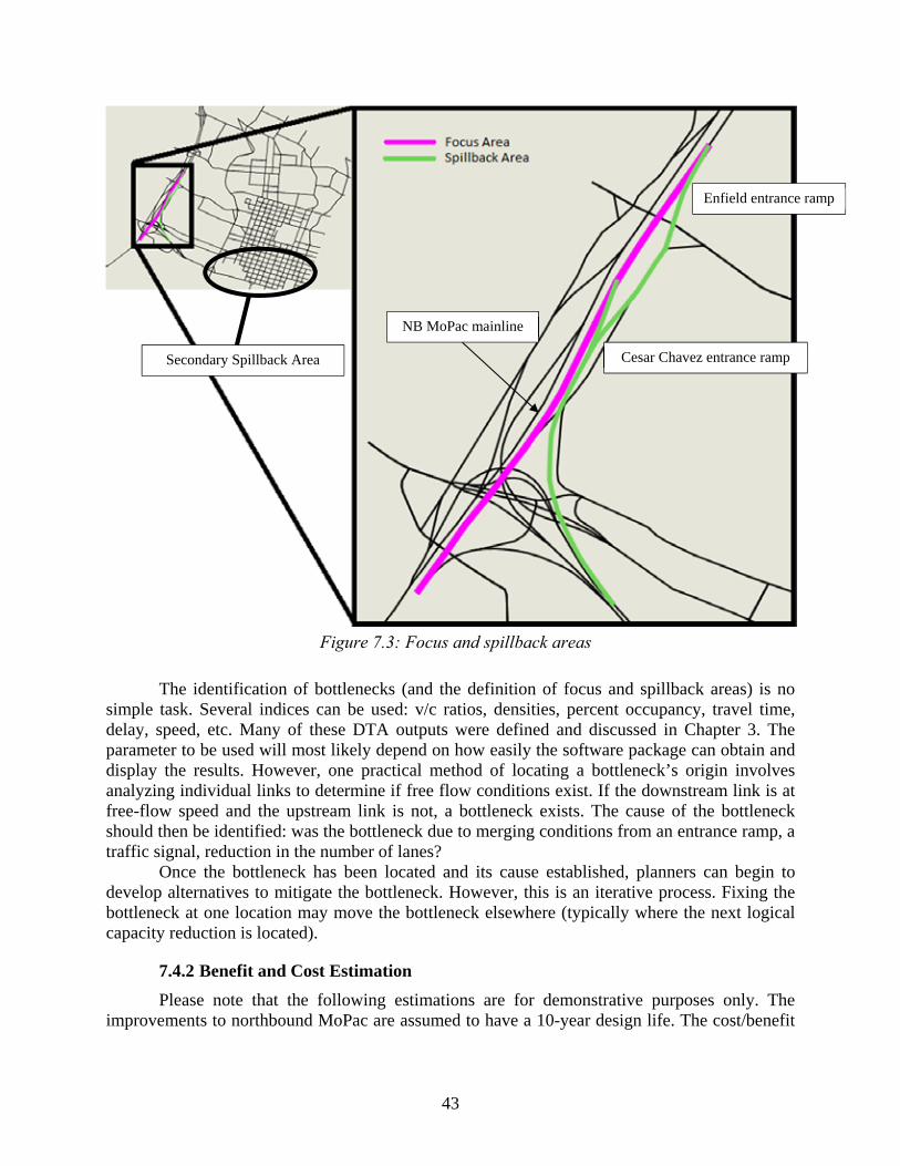
43
Figure 7.3: Focus and spillback areas
The identification of bottlenecks (and the definition of focus and spillback areas) is no simple task. Several indices can be used: v/c ratios, densities, percent occupancy, travel time, delay, speed, etc. Many of these DTA outputs were defined and discussed in Chapter 3. The parameter to be used will most likely depend on how easily the software package can obtain and display the results. However, one practical method of locating a bottleneck’s origin involves analyzing individual links to determine if free flow conditions exist. If the downstream link is at free-flow speed and the upstream link is not, a bottleneck exists. The cause of the bottleneck should then be identified: was the bottleneck due to merging conditions from an entrance ramp, a traffic signal, reduction in the number of lanes?
Once the bottleneck has been located and its cause established, planners can begin to develop alternatives to mitigate the bottleneck. However, this is an iterative process. Fixing the bottleneck at one location may move the bottleneck elsewhere (typically where the next logical capacity reduction is located).
7.4.2 Benefit and Cost Estimation
Please note that the following estimations are for demonstrative purposes only. The improvements to northbound MoPac are assumed to have a 10-year design life. The cost/benefit
Enfield entrance ramp
Cesar Chavez entrance ramp
NB MoPac mainline
Secondary Spillback Area
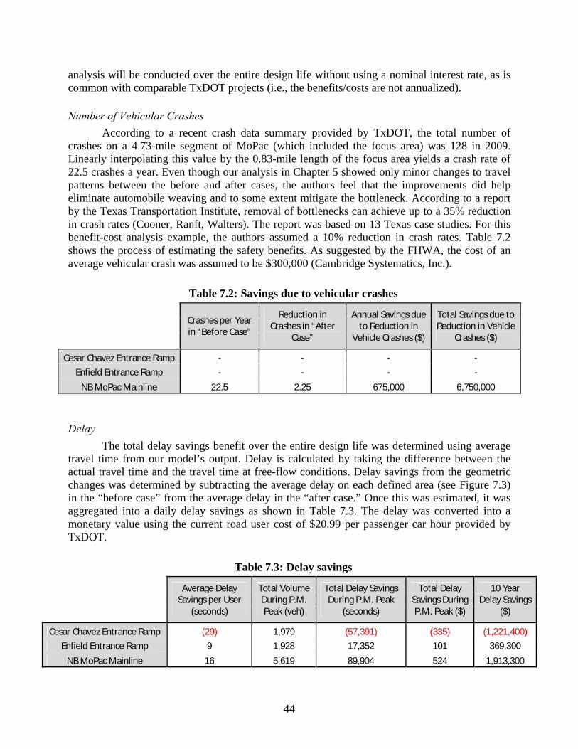
44
analysis will be conducted over the entire design life without using a nominal interest rate, as is common with comparable TxDOT projects (i.e., the benefits/costs are not annualized).
Number of Vehicular Crashes
According to a recent crash data summary provided by TxDOT, the total number of crashes on a 4.73-mile segment of MoPac (which included the focus area) was 128 in 2009. Linearly interpolating this value by the 0.83-mile length of the focus area yields a crash rate of 22.5 crashes a year. Even though our analysis in Chapter 5 showed only minor changes to travel patterns between the before and after cases, the authors feel that the improvements did help eliminate automobile weaving and to some extent mitigate the bottleneck. According to a report by the Texas Transportation Institute, removal of bottlenecks can achieve up to a 35% reduction in crash rates (Cooner, Ranft, Walters). The report was based on 13 Texas case studies. For this benefit-cost analysis example, the authors assumed a 10% reduction in crash rates. Table 7.2 shows the process of estimating the safety benefits. As suggested by the FHWA, the cost of an average vehicular crash was assumed to be $300,000 (Cambridge Systematics, Inc.).
Table 7.2: Savings due to vehicular crashes
Crashes per Year in “Before Case”
Reduction in Crashes in “After
Case”
Annual Savings due to Reduction in
Vehicle Crashes ($)
Total Savings due to Reduction in Vehicle
Crashes ($)
Cesar Chavez Entrance Ramp - - - - Enfield Entrance Ramp - - - -
NB MoPac Mainline 22.5 2.25 675,000 6,750,000
Delay
The total delay savings benefit over the entire design life was determined using average travel time from our model’s output. Delay is calculated by taking the difference between the actual travel time and the travel time at free-flow conditions. Delay savings from the geometric changes was determined by subtracting the average delay on each defined area (see Figure 7.3) in the “before case” from the average delay in the “after case.” Once this was estimated, it was aggregated into a daily delay savings as shown in Table 7.3. The delay was converted into a monetary value using the current road user cost of $20.99 per passenger car hour provided by TxDOT.
Table 7.3: Delay savings
Average Delay Savings per User
(seconds)
Total Volume During P.M. Peak (veh)
Total Delay Savings During P.M. Peak
(seconds)
Total Delay Savings During P.M. Peak ($)
10 Year Delay Savings
($)
Cesar Chavez Entrance Ramp (29) 1,979 (57,391) (335) (1,221,400) Enfield Entrance Ramp 9 1,928 17,352 101 369,300
NB MoPac Mainline 16 5,619 89,904 524 1,913,300
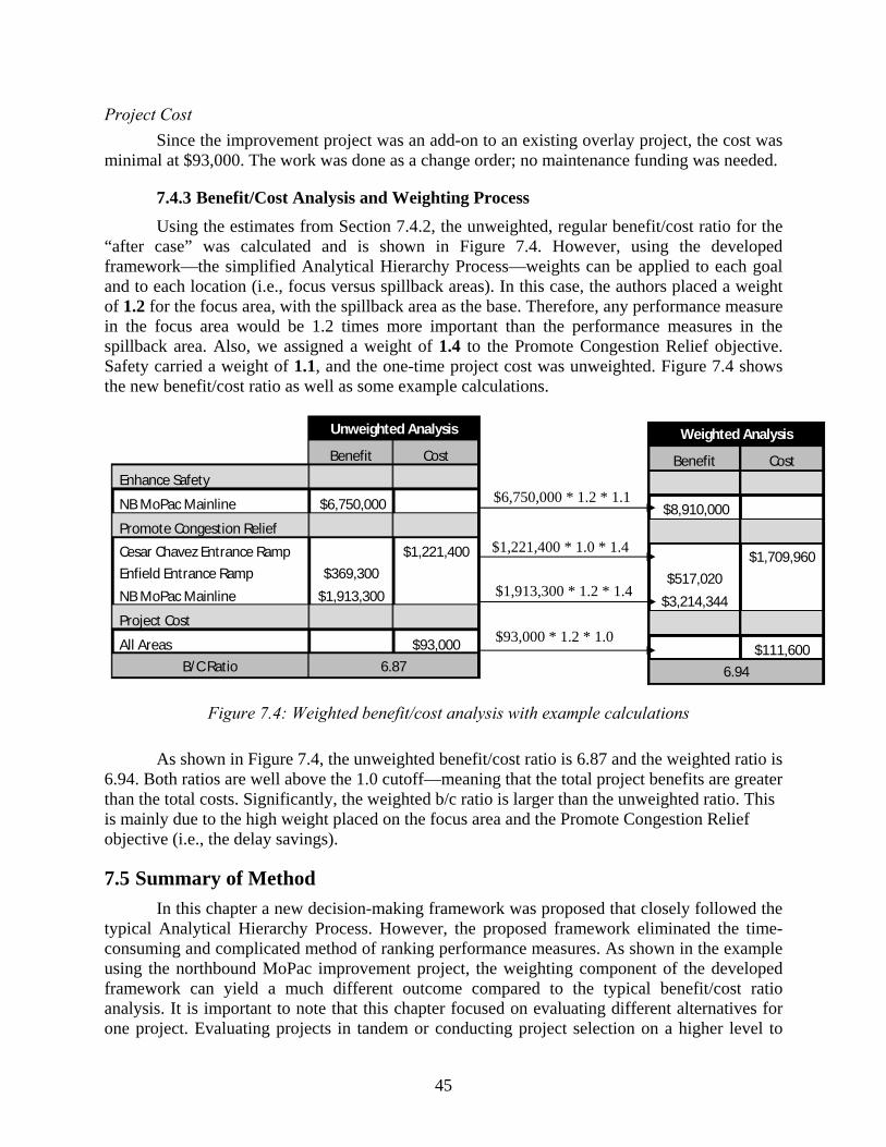
45
Project Cost
Since the improvement project was an add-on to an existing overlay project, the cost was minimal at $93,000. The work was done as a change order; no maintenance funding was needed.
7.4.3 Benefit/Cost Analysis and Weighting Process
Using the estimates from Section 7.4.2, the unweighted, regular benefit/cost ratio for the “after case” was calculated and is shown in Figure 7.4. However, using the developed framework—the simplified Analytical Hierarchy Process—weights can be applied to each goal and to each location (i.e., focus versus spillback areas). In this case, the authors placed a weight of 1.2 for the focus area, with the spillback area as the base. Therefore, any performance measure in the focus area would be 1.2 times more important than the performance measures in the spillback area. Also, we assigned a weight of 1.4 to the Promote Congestion Relief objective. Safety carried a weight of 1.1, and the one-time project cost was unweighted. Figure 7.4 shows the new benefit/cost ratio as well as some example calculations.
Figure 7.4: Weighted benefit/cost analysis with example calculations
As shown in Figure 7.4, the unweighted benefit/cost ratio is 6.87 and the weighted ratio is 6.94. Both ratios are well above the 1.0 cutoff—meaning that the total project benefits are greater than the total costs. Significantly, the weighted b/c ratio is larger than the unweighted ratio. This is mainly due to the high weight placed on the focus area and the Promote Congestion Relief objective (i.e., the delay savings).
7.5 Summary of Method
In this chapter a new decision-making framework was proposed that closely followed the typical Analytical Hierarchy Process. However, the proposed framework eliminated the time-consuming and complicated method of ranking performance measures. As shown in the example using the northbound MoPac improvement project, the weighting component of the developed framework can yield a much different outcome compared to the typical benefit/cost ratio analysis. It is important to note that this chapter focused on evaluating different alternatives for one project. Evaluating projects in tandem or conducting project selection on a higher level to
Unweighted Analysis
Benefit Cost
Enhance Safety
NB MoPac Mainline $6,750,000
Promote Congestion Relief
Cesar Chavez Entrance Ramp $1,221,400 Enfield Entrance Ramp $369,300 NB MoPac Mainline $1,913,300
Project Cost
All Areas $93,000 B/C Ratio 6.87
Weighted Analysis
Benefit Cost
$8,910,000
$1,709,960 $517,020
$3,214,344
$111,600 6.94
$6,750,000 * 1.2 * 1.1
$1,221,400 * 1.0 * 1.4
$1,913,300 * 1.2 * 1.4
$93,000 * 1.2 * 1.0

46
take advantage of synergy effects between different projects is important and should be considered at any public transportation agency.
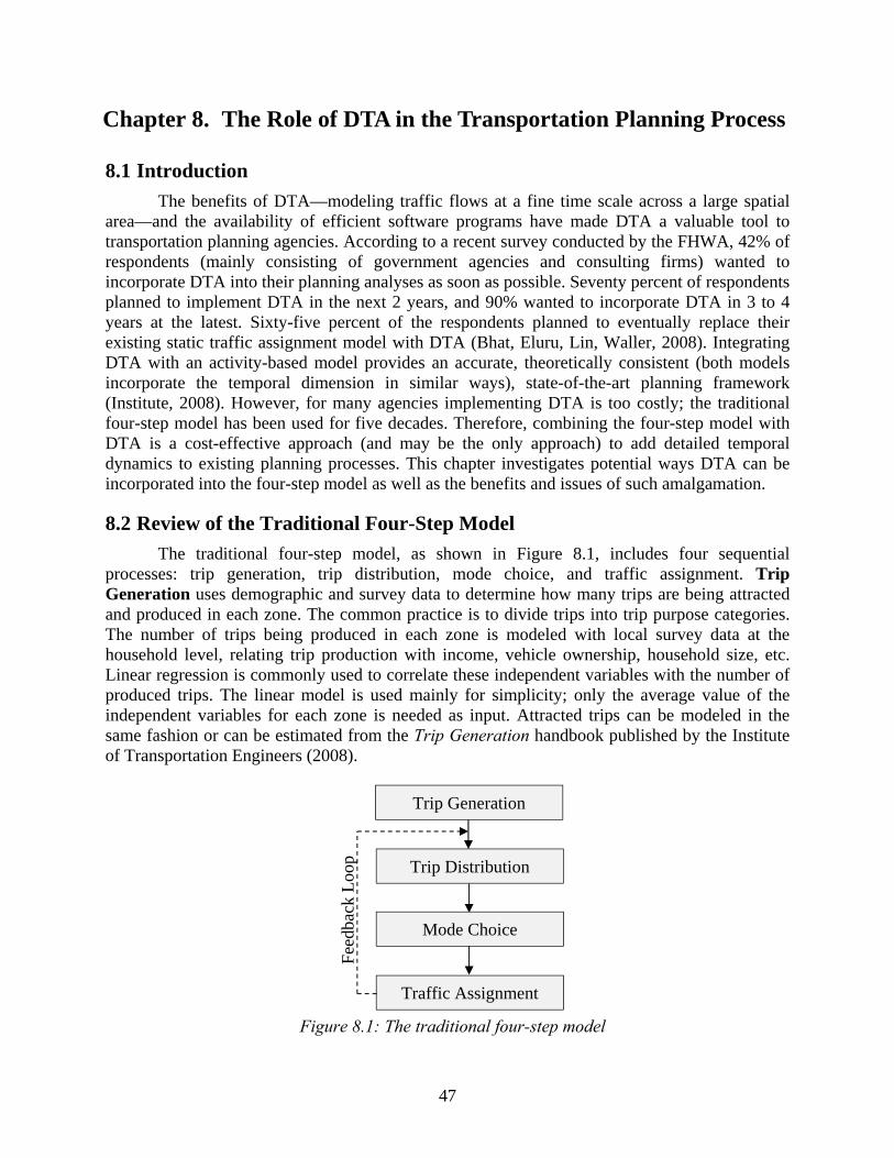
47
Chapter 8. The Role of DTA in the Transportation Planning Process
8.1 Introduction
The benefits of DTA—modeling traffic flows at a fine time scale across a large spatial area—and the availability of efficient software programs have made DTA a valuable tool to transportation planning agencies. According to a recent survey conducted by the FHWA, 42% of respondents (mainly consisting of government agencies and consulting firms) wanted to incorporate DTA into their planning analyses as soon as possible. Seventy percent of respondents planned to implement DTA in the next 2 years, and 90% wanted to incorporate DTA in 3 to 4 years at the latest. Sixty-five percent of the respondents planned to eventually replace their existing static traffic assignment model with DTA (Bhat, Eluru, Lin, Waller, 2008). Integrating DTA with an activity-based model provides an accurate, theoretically consistent (both models incorporate the temporal dimension in similar ways), state-of-the-art planning framework (Institute, 2008). However, for many agencies implementing DTA is too costly; the traditional four-step model has been used for five decades. Therefore, combining the four-step model with DTA is a cost-effective approach (and may be the only approach) to add detailed temporal dynamics to existing planning processes. This chapter investigates potential ways DTA can be incorporated into the four-step model as well as the benefits and issues of such amalgamation.
8.2 Review of the Traditional Four-Step Model
The traditional four-step model, as shown in Figure 8.1, includes four sequential processes: trip generation, trip distribution, mode choice, and traffic assignment. Trip Generation uses demographic and survey data to determine how many trips are being attracted and produced in each zone. The common practice is to divide trips into trip purpose categories. The number of trips being produced in each zone is modeled with local survey data at the household level, relating trip production with income, vehicle ownership, household size, etc. Linear regression is commonly used to correlate these independent variables with the number of produced trips. The linear model is used mainly for simplicity; only the average value of the independent variables for each zone is needed as input. Attracted trips can be modeled in the same fashion or can be estimated from the Trip Generation handbook published by the Institute of Transportation Engineers (2008).
Figure 8.1: The traditional four-step model
Trip Generation
Trip Distribution
Mode Choice
Traffic Assignment
Fee
dbac
k L
oop
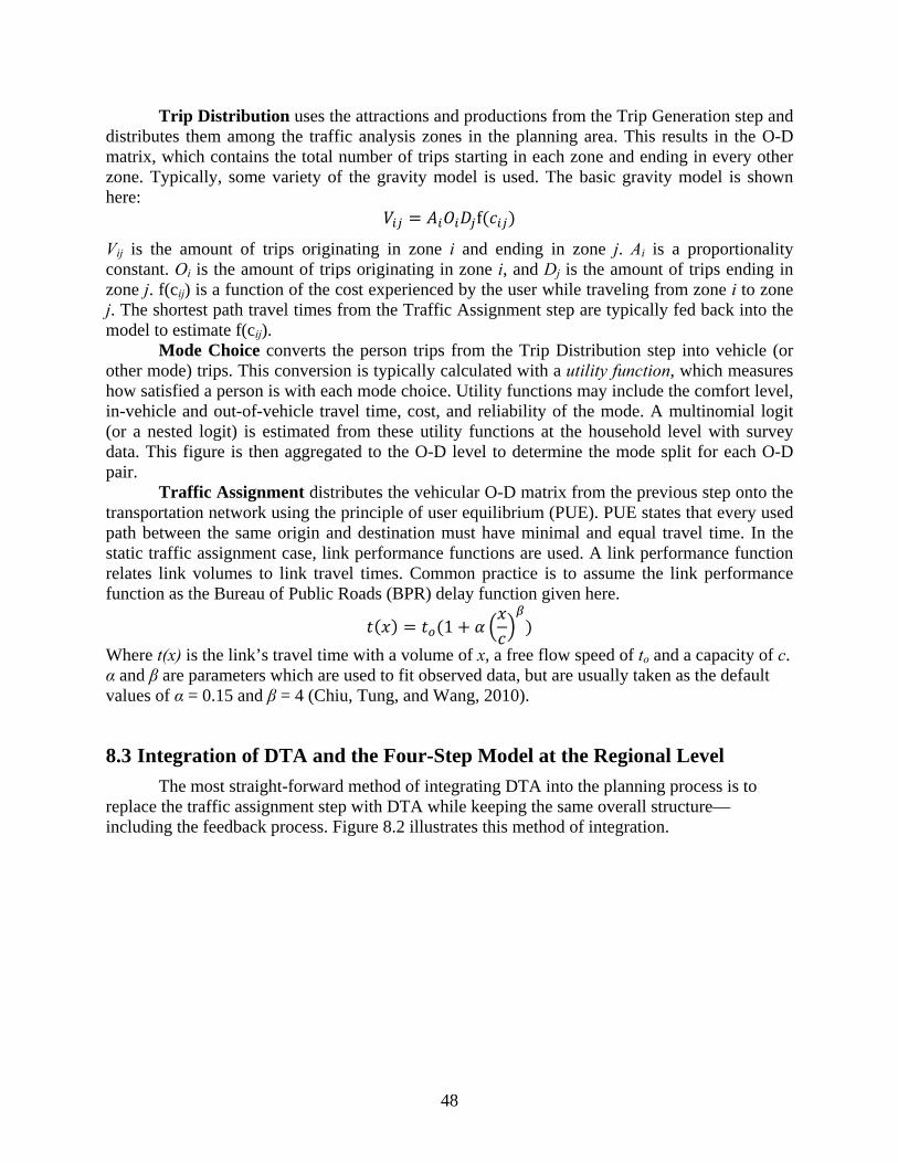
48
Trip Distribution uses the attractions and productions from the Trip Generation step and distributes them among the traffic analysis zones in the planning area. This results in the O-D matrix, which contains the total number of trips starting in each zone and ending in every other zone. Typically, some variety of the gravity model is used. The basic gravity model is shown here: = f( ) Vij is the amount of trips originating in zone i and ending in zone j. Ai is a proportionality constant. Oi is the amount of trips originating in zone i, and Dj is the amount of trips ending in zone j. f(cij) is a function of the cost experienced by the user while traveling from zone i to zone j. The shortest path travel times from the Traffic Assignment step are typically fed back into the model to estimate f(cij).
Mode Choice converts the person trips from the Trip Distribution step into vehicle (or other mode) trips. This conversion is typically calculated with a utility function, which measures how satisfied a person is with each mode choice. Utility functions may include the comfort level, in-vehicle and out-of-vehicle travel time, cost, and reliability of the mode. A multinomial logit (or a nested logit) is estimated from these utility functions at the household level with survey data. This figure is then aggregated to the O-D level to determine the mode split for each O-D pair.
Traffic Assignment distributes the vehicular O-D matrix from the previous step onto the transportation network using the principle of user equilibrium (PUE). PUE states that every used path between the same origin and destination must have minimal and equal travel time. In the static traffic assignment case, link performance functions are used. A link performance function relates link volumes to link travel times. Common practice is to assume the link performance function as the Bureau of Public Roads (BPR) delay function given here. ( ) = (1 + ) Where t(x) is the link’s travel time with a volume of x, a free flow speed of to and a capacity of c. α and β are parameters which are used to fit observed data, but are usually taken as the default values of α = 0.15 and β = 4 (Chiu, Tung, and Wang, 2010).
8.3 Integration of DTA and the Four-Step Model at the Regional Level
The most straight-forward method of integrating DTA into the planning process is to replace the traffic assignment step with DTA while keeping the same overall structure—including the feedback process. Figure 8.2 illustrates this method of integration.
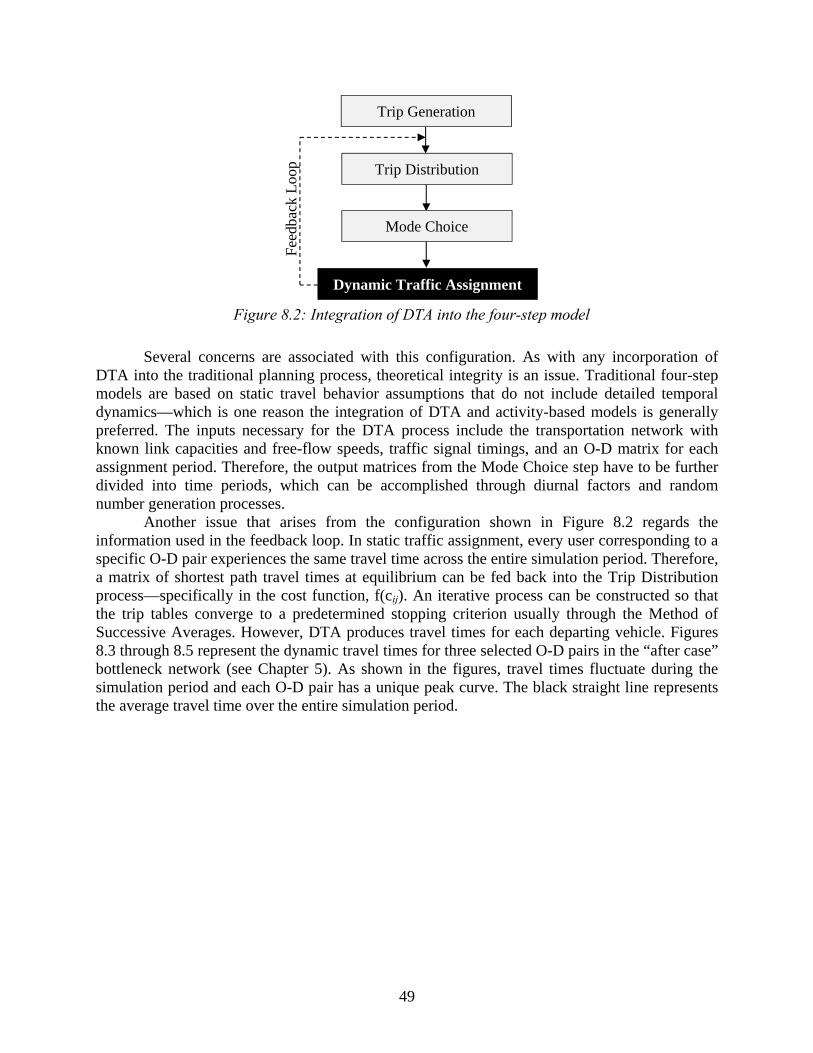
49
Figure 8.2: Integration of DTA into the four-step model
Several concerns are associated with this configuration. As with any incorporation of DTA into the traditional planning process, theoretical integrity is an issue. Traditional four-step models are based on static travel behavior assumptions that do not include detailed temporal dynamics—which is one reason the integration of DTA and activity-based models is generally preferred. The inputs necessary for the DTA process include the transportation network with known link capacities and free-flow speeds, traffic signal timings, and an O-D matrix for each assignment period. Therefore, the output matrices from the Mode Choice step have to be further divided into time periods, which can be accomplished through diurnal factors and random number generation processes.
Another issue that arises from the configuration shown in Figure 8.2 regards the information used in the feedback loop. In static traffic assignment, every user corresponding to a specific O-D pair experiences the same travel time across the entire simulation period. Therefore, a matrix of shortest path travel times at equilibrium can be fed back into the Trip Distribution process—specifically in the cost function, f(cij). An iterative process can be constructed so that the trip tables converge to a predetermined stopping criterion usually through the Method of Successive Averages. However, DTA produces travel times for each departing vehicle. Figures 8.3 through 8.5 represent the dynamic travel times for three selected O-D pairs in the “after case” bottleneck network (see Chapter 5). As shown in the figures, travel times fluctuate during the simulation period and each O-D pair has a unique peak curve. The black straight line represents the average travel time over the entire simulation period.
Trip Generation
Trip Distribution
Mode Choice
Dynamic Traffic Assignment F
eedb
ack
Loo
p
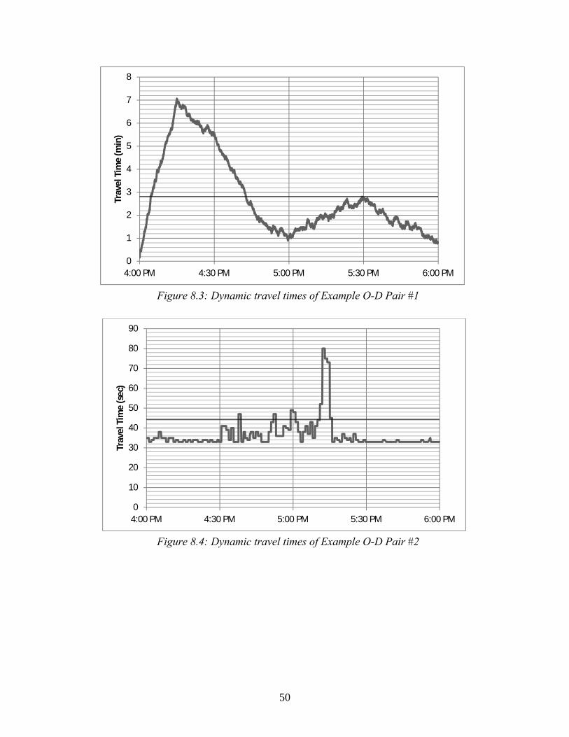
50
Figure 8.3: Dynamic travel times of Example O-D Pair #1
Figure 8.4: Dynamic travel times of Example O-D Pair #2
0
1
2
3
4
5
6
7
8
4:00 PM 4:30 PM 5:00 PM 5:30 PM 6:00 PM
Trav
el T
ime
(min
)
0
10
20
30
40
50
60
70
80
90
4:00 PM 4:30 PM 5:00 PM 5:30 PM 6:00 PM
Trav
el T
ime
(sec
)
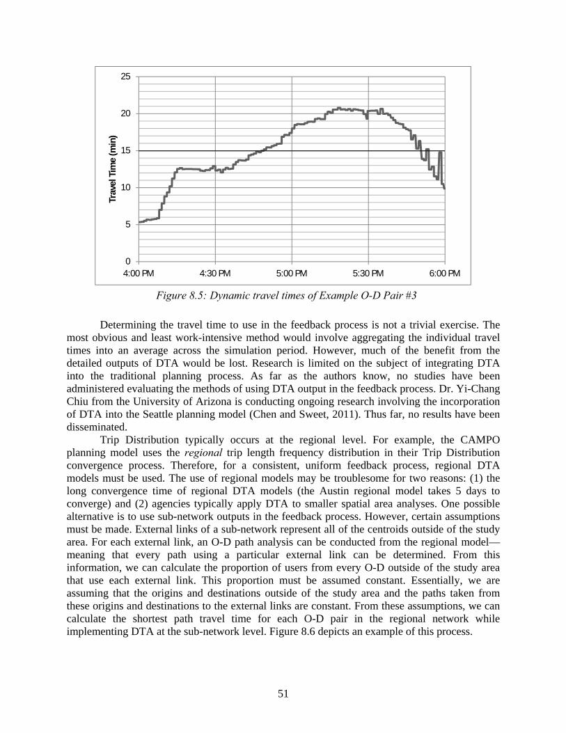
51
Figure 8.5: Dynamic travel times of Example O-D Pair #3
Determining the travel time to use in the feedback process is not a trivial exercise. The most obvious and least work-intensive method would involve aggregating the individual travel times into an average across the simulation period. However, much of the benefit from the detailed outputs of DTA would be lost. Research is limited on the subject of integrating DTA into the traditional planning process. As far as the authors know, no studies have been administered evaluating the methods of using DTA output in the feedback process. Dr. Yi-Chang Chiu from the University of Arizona is conducting ongoing research involving the incorporation of DTA into the Seattle planning model (Chen and Sweet, 2011). Thus far, no results have been disseminated.
Trip Distribution typically occurs at the regional level. For example, the CAMPO planning model uses the regional trip length frequency distribution in their Trip Distribution convergence process. Therefore, for a consistent, uniform feedback process, regional DTA models must be used. The use of regional models may be troublesome for two reasons: (1) the long convergence time of regional DTA models (the Austin regional model takes 5 days to converge) and (2) agencies typically apply DTA to smaller spatial area analyses. One possible alternative is to use sub-network outputs in the feedback process. However, certain assumptions must be made. External links of a sub-network represent all of the centroids outside of the study area. For each external link, an O-D path analysis can be conducted from the regional model—meaning that every path using a particular external link can be determined. From this information, we can calculate the proportion of users from every O-D outside of the study area that use each external link. This proportion must be assumed constant. Essentially, we are assuming that the origins and destinations outside of the study area and the paths taken from these origins and destinations to the external links are constant. From these assumptions, we can calculate the shortest path travel time for each O-D pair in the regional network while implementing DTA at the sub-network level. Figure 8.6 depicts an example of this process.
0
5
10
15
20
25
4:00 PM 4:30 PM 5:00 PM 5:30 PM 6:00 PM
Trav
el T
ime
(min
)
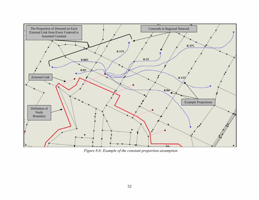
52
Figure 8.6: Example of the constant proportion assumption
External Link
Definition of Study
Boundary
Centroids in Regional Network The Proportion of Demand on Each External Link from Every Centroid is
Assumed Constant
0.25
0.125
0.125
0.375
0.04
0.02
0.065
Example Proportions
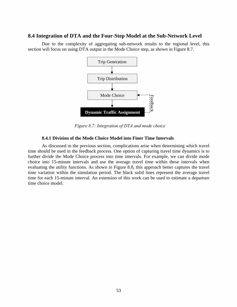
53
8.4 Integration of DTA and the Four-Step Model at the Sub-Network Level
Due to the complexity of aggregating sub-network results to the regional level, this section will focus on using DTA output in the Mode Choice step, as shown in Figure 8.7.
Figure 8.7: Integration of DTA and mode choice
8.4.1 Division of the Mode Choice Model into Finer Time Intervals
As discussed in the previous section, complications arise when determining which travel time should be used in the feedback process. One option of capturing travel time dynamics is to further divide the Mode Choice process into time intervals. For example, we can divide mode choice into 15-minute intervals and use the average travel time within these intervals when evaluating the utility functions. As shown in Figure 8.8, this approach better captures the travel time variation within the simulation period. The black solid lines represent the average travel time for each 15-minute interval. An extension of this work can be used to estimate a departure time choice model.
Trip Generation
Trip Distribution
Mode Choice
Dynamic Traffic Assignment
Feedback
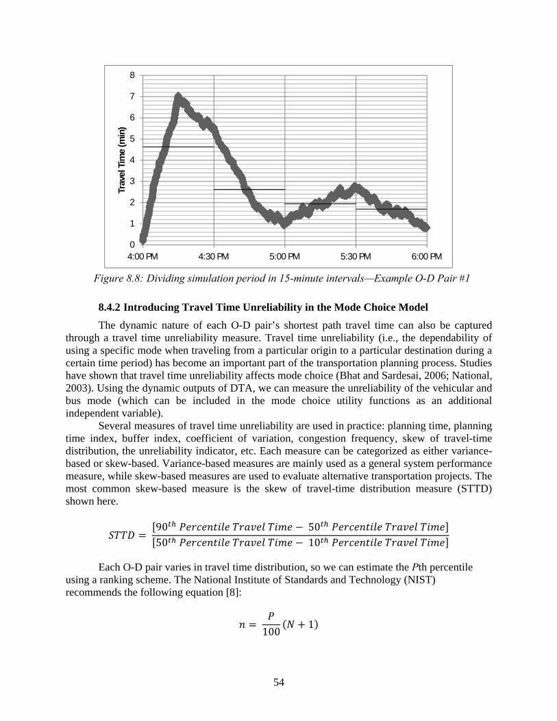
54
Figure 8.8: Dividing simulation period in 15-minute intervals—Example O-D Pair #1
8.4.2 Introducing Travel Time Unreliability in the Mode Choice Model
The dynamic nature of each O-D pair’s shortest path travel time can also be captured through a travel time unreliability measure. Travel time unreliability (i.e., the dependability of using a specific mode when traveling from a particular origin to a particular destination during a certain time period) has become an important part of the transportation planning process. Studies have shown that travel time unreliability affects mode choice (Bhat and Sardesai, 2006; National, 2003). Using the dynamic outputs of DTA, we can measure the unreliability of the vehicular and bus mode (which can be included in the mode choice utility functions as an additional independent variable).
Several measures of travel time unreliability are used in practice: planning time, planning time index, buffer index, coefficient of variation, congestion frequency, skew of travel-time distribution, the unreliability indicator, etc. Each measure can be categorized as either variance-based or skew-based. Variance-based measures are mainly used as a general system performance measure, while skew-based measures are used to evaluate alternative transportation projects. The most common skew-based measure is the skew of travel-time distribution measure (STTD) shown here.
= 90 −50 50 −10
Each O-D pair varies in travel time distribution, so we can estimate the Pth percentile
using a ranking scheme. The National Institute of Standards and Technology (NIST) recommends the following equation [8]:
=100 ( + 1)
0
1
2
3
4
5
6
7
8
4:00 PM 4:30 PM 5:00 PM 5:30 PM 6:00 PM
Trav
el T
ime
(min
)
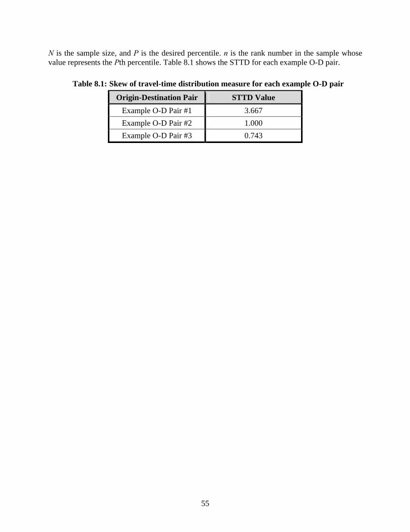
55
N is the sample size, and P is the desired percentile. n is the rank number in the sample whose value represents the Pth percentile. Table 8.1 shows the STTD for each example O-D pair.
Table 8.1: Skew of travel-time distribution measure for each example O-D pair
Origin-Destination Pair STTD Value
Example O-D Pair #1 3.667
Example O-D Pair #2 1.000
Example O-D Pair #3 0.743

56
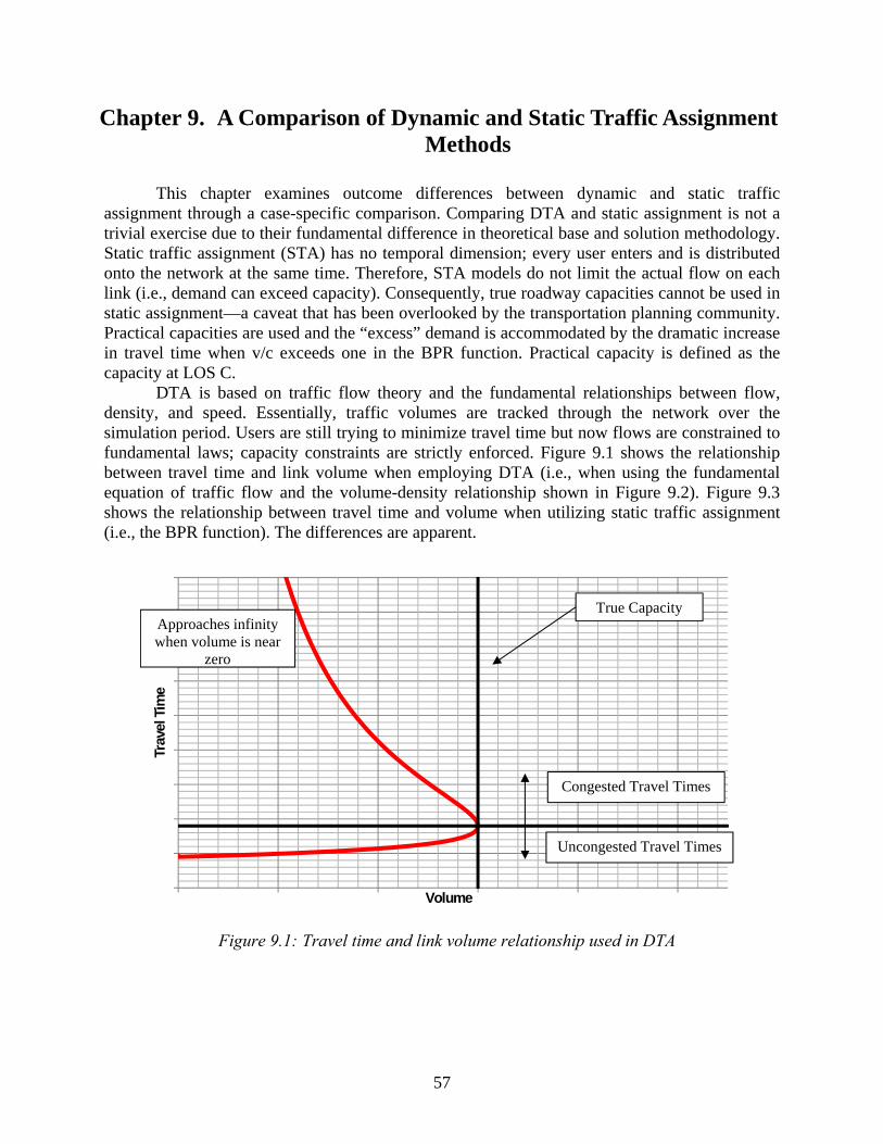
57
Chapter 9. A Comparison of Dynamic and Static Traffic Assignment Methods
This chapter examines outcome differences between dynamic and static traffic assignment through a case-specific comparison. Comparing DTA and static assignment is not a trivial exercise due to their fundamental difference in theoretical base and solution methodology. Static traffic assignment (STA) has no temporal dimension; every user enters and is distributed onto the network at the same time. Therefore, STA models do not limit the actual flow on each link (i.e., demand can exceed capacity). Consequently, true roadway capacities cannot be used in static assignment—a caveat that has been overlooked by the transportation planning community. Practical capacities are used and the “excess” demand is accommodated by the dramatic increase in travel time when v/c exceeds one in the BPR function. Practical capacity is defined as the capacity at LOS C.
DTA is based on traffic flow theory and the fundamental relationships between flow, density, and speed. Essentially, traffic volumes are tracked through the network over the simulation period. Users are still trying to minimize travel time but now flows are constrained to fundamental laws; capacity constraints are strictly enforced. Figure 9.1 shows the relationship between travel time and link volume when employing DTA (i.e., when using the fundamental equation of traffic flow and the volume-density relationship shown in Figure 9.2). Figure 9.3 shows the relationship between travel time and volume when utilizing static traffic assignment (i.e., the BPR function). The differences are apparent.
Figure 9.1: Travel time and link volume relationship used in DTA
Trav
el T
ime
Volume
True Capacity
Congested Travel Times
Uncongested Travel Times
Approaches infinity when volume is near
zero
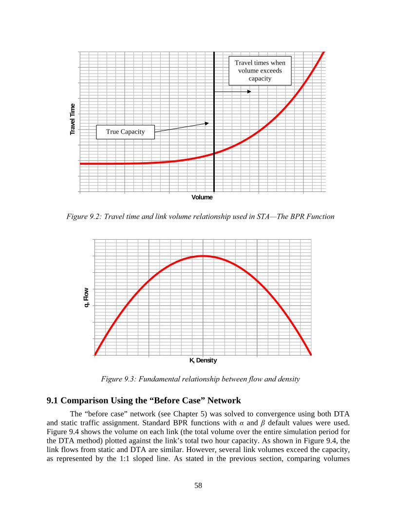
58
Figure 9.2: Travel time and link volume relationship used in STA—The BPR Function
Figure 9.3: Fundamental relationship between flow and density
9.1 Comparison Using the “Before Case” Network
The “before case” network (see Chapter 5) was solved to convergence using both DTA and static traffic assignment. Standard BPR functions with α and β default values were used. Figure 9.4 shows the volume on each link (the total volume over the entire simulation period for the DTA method) plotted against the link’s total two hour capacity. As shown in Figure 9.4, the link flows from static and DTA are similar. However, several link volumes exceed the capacity, as represented by the 1:1 sloped line. As stated in the previous section, comparing volumes
Trav
el T
ime
Volume
True Capacity
Travel times when volume exceeds
capacityq,
Flo
w
K, Density

59
between the two assignment methods is difficult, since vehicular flow from STA represents link demand (the number of vehicles wishing to use the link), not necessarily the number of vehicles actually forecasted to use the link.
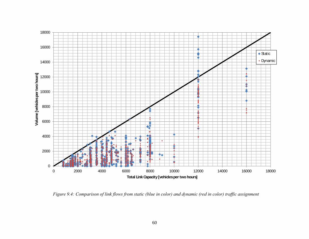
60
Figure 9.4: Comparison of link flows from static (blue in color) and dynamic (red in color) traffic assignment
0
2000
4000
6000
8000
10000
12000
14000
16000
18000
0 2000 4000 6000 8000 10000 12000 14000 16000 18000
Volu
me
[veh
icle
s per
two
hour
s]
Total Link Capacity [vehicles per two hours]
Static
Dynamic
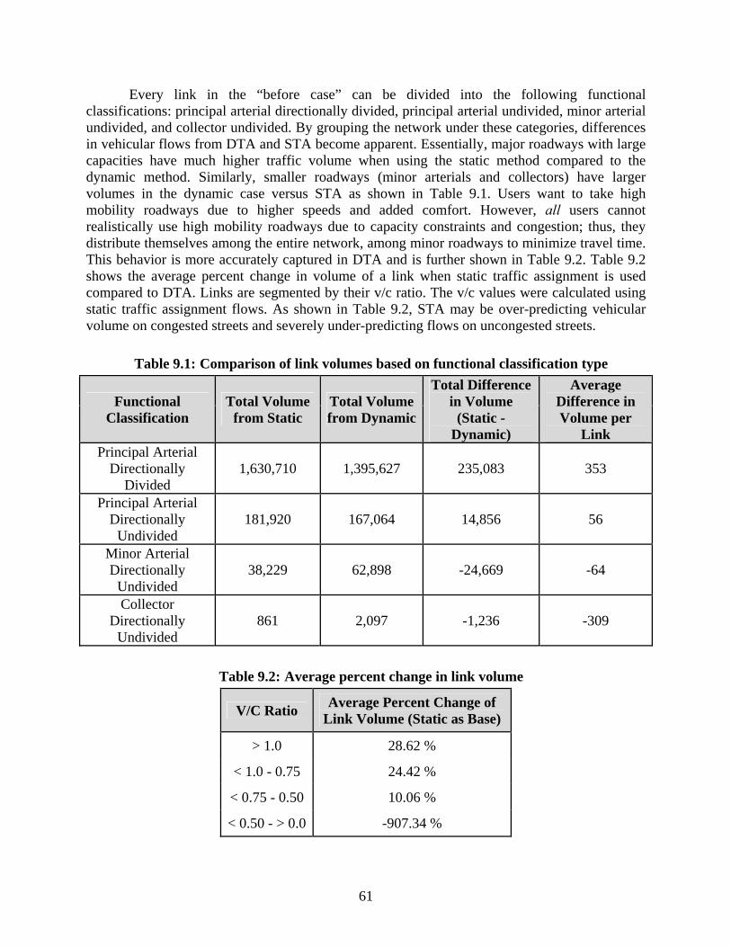
61
Every link in the “before case” can be divided into the following functional classifications: principal arterial directionally divided, principal arterial undivided, minor arterial undivided, and collector undivided. By grouping the network under these categories, differences in vehicular flows from DTA and STA become apparent. Essentially, major roadways with large capacities have much higher traffic volume when using the static method compared to the dynamic method. Similarly, smaller roadways (minor arterials and collectors) have larger volumes in the dynamic case versus STA as shown in Table 9.1. Users want to take high mobility roadways due to higher speeds and added comfort. However, all users cannot realistically use high mobility roadways due to capacity constraints and congestion; thus, they distribute themselves among the entire network, among minor roadways to minimize travel time. This behavior is more accurately captured in DTA and is further shown in Table 9.2. Table 9.2 shows the average percent change in volume of a link when static traffic assignment is used compared to DTA. Links are segmented by their v/c ratio. The v/c values were calculated using static traffic assignment flows. As shown in Table 9.2, STA may be over-predicting vehicular volume on congested streets and severely under-predicting flows on uncongested streets.
Table 9.1: Comparison of link volumes based on functional classification type
Functional Classification
Total Volume from Static
Total Volume from Dynamic
Total Difference in Volume
(Static - Dynamic)
Average Difference in Volume per
Link Principal Arterial
Directionally Divided
1,630,710 1,395,627 235,083 353
Principal Arterial Directionally
Undivided 181,920 167,064 14,856 56
Minor Arterial Directionally
Undivided 38,229 62,898 -24,669 -64
Collector Directionally
Undivided 861 2,097 -1,236 -309
Table 9.2: Average percent change in link volume
V/C Ratio Average Percent Change of
Link Volume (Static as Base)
> 1.0 28.62 %
< 1.0 - 0.75 24.42 %
< 0.75 - 0.50 10.06 %
< 0.50 - > 0.0 -907.34 %
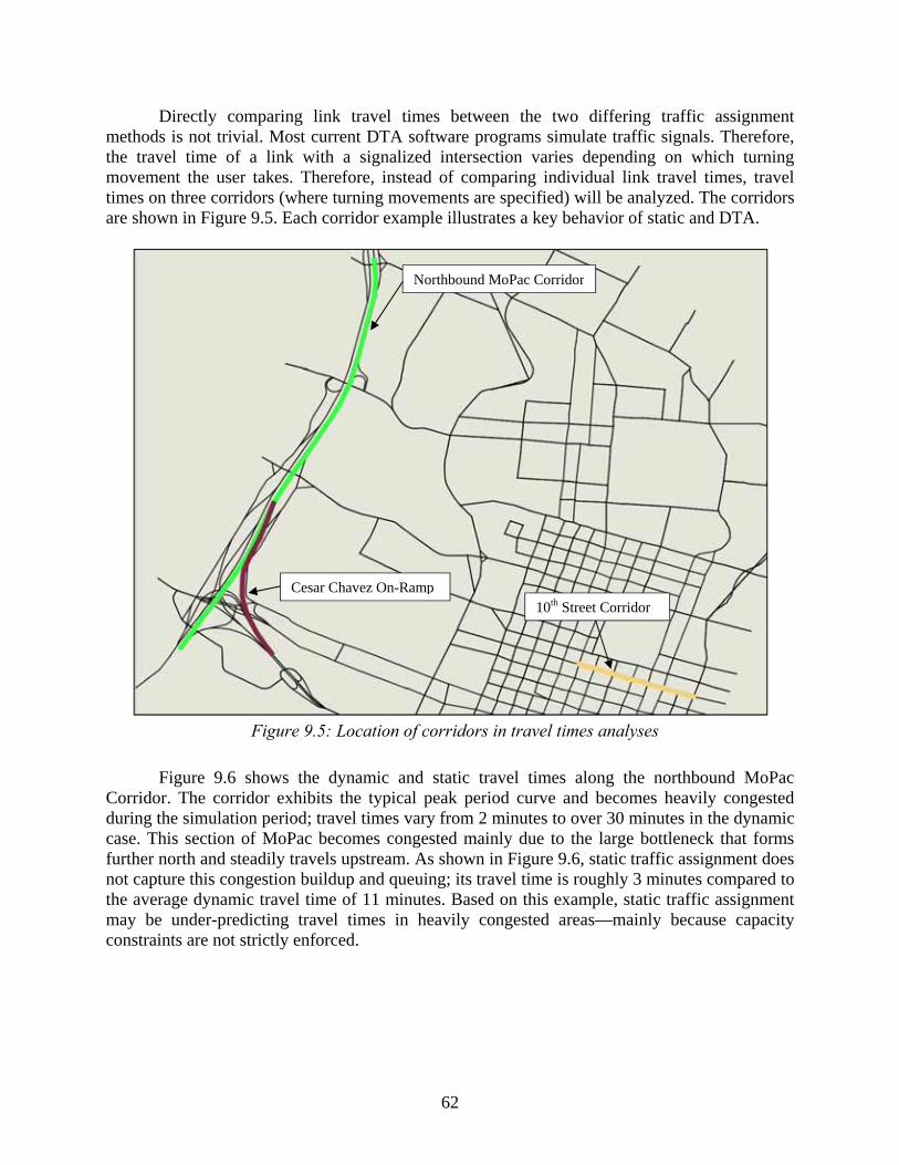
62
Directly comparing link travel times between the two differing traffic assignment methods is not trivial. Most current DTA software programs simulate traffic signals. Therefore, the travel time of a link with a signalized intersection varies depending on which turning movement the user takes. Therefore, instead of comparing individual link travel times, travel times on three corridors (where turning movements are specified) will be analyzed. The corridors are shown in Figure 9.5. Each corridor example illustrates a key behavior of static and DTA.
Figure 9.5: Location of corridors in travel times analyses
Figure 9.6 shows the dynamic and static travel times along the northbound MoPac Corridor. The corridor exhibits the typical peak period curve and becomes heavily congested during the simulation period; travel times vary from 2 minutes to over 30 minutes in the dynamic case. This section of MoPac becomes congested mainly due to the large bottleneck that forms further north and steadily travels upstream. As shown in Figure 9.6, static traffic assignment does not capture this congestion buildup and queuing; its travel time is roughly 3 minutes compared to the average dynamic travel time of 11 minutes. Based on this example, static traffic assignment may be under-predicting travel times in heavily congested areas—mainly because capacity constraints are not strictly enforced.
Northbound MoPac Corridor
Cesar Chavez On-Ramp10th Street Corridor
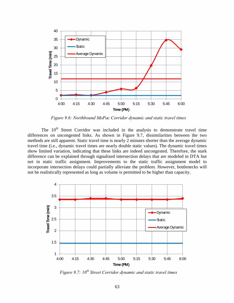
63
Figure 9.6: Northbound MoPac Corridor dynamic and static travel times
The 10th Street Corridor was included in the analysis to demonstrate travel time differences on uncongested links. As shown in Figure 9.7, dissimilarities between the two methods are still apparent. Static travel time is nearly 2 minutes shorter than the average dynamic travel time (i.e., dynamic travel times are nearly double static values). The dynamic travel times show limited variation, indicating that these links are indeed uncongested. Therefore, the stark difference can be explained through signalized intersection delays that are modeled in DTA but not in static traffic assignment. Improvements to the static traffic assignment model to incorporate intersection delays could partially alleviate the problem. However, bottlenecks will not be realistically represented as long as volume is permitted to be higher than capacity.
Figure 9.7: 10th Street Corridor dynamic and static travel times
0
5
10
15
20
25
30
35
40
4:00 4:15 4:30 4:45 5:00 5:15 5:30 5:45 6:00
Trav
el T
ime
(min
)
Time (PM)
Dynamic
Static
Average Dynamic
1
1.5
2
2.5
3
3.5
4
4:00 4:15 4:30 4:45 5:00 5:15 5:30 5:45 6:00
Trav
el T
ime
(min
)
Time (PM)
Dynamic
Static
Average Dynamic
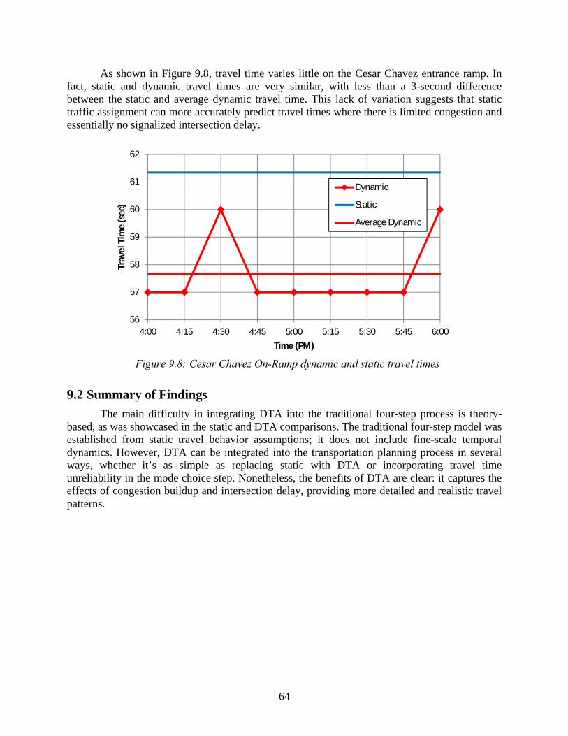
64
As shown in Figure 9.8, travel time varies little on the Cesar Chavez entrance ramp. In fact, static and dynamic travel times are very similar, with less than a 3-second difference between the static and average dynamic travel time. This lack of variation suggests that static traffic assignment can more accurately predict travel times where there is limited congestion and essentially no signalized intersection delay.
Figure 9.8: Cesar Chavez On-Ramp dynamic and static travel times
9.2 Summary of Findings
The main difficulty in integrating DTA into the traditional four-step process is theory-based, as was showcased in the static and DTA comparisons. The traditional four-step model was established from static travel behavior assumptions; it does not include fine-scale temporal dynamics. However, DTA can be integrated into the transportation planning process in several ways, whether it’s as simple as replacing static with DTA or incorporating travel time unreliability in the mode choice step. Nonetheless, the benefits of DTA are clear: it captures the effects of congestion buildup and intersection delay, providing more detailed and realistic travel patterns.
56
57
58
59
60
61
62
4:00 4:15 4:30 4:45 5:00 5:15 5:30 5:45 6:00
Trav
el T
ime
(sec
)
Time (PM)
Dynamic
Static
Average Dynamic
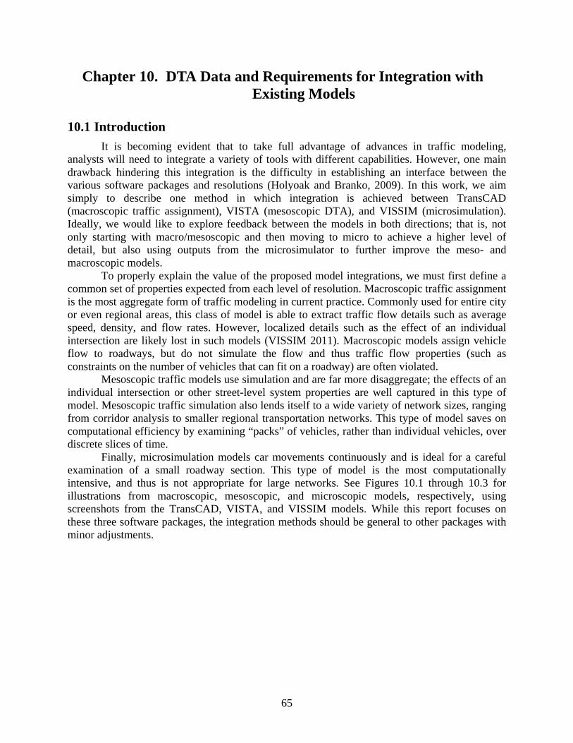
65
Chapter 10. DTA Data and Requirements for Integration with Existing Models
10.1 Introduction
It is becoming evident that to take full advantage of advances in traffic modeling, analysts will need to integrate a variety of tools with different capabilities. However, one main drawback hindering this integration is the difficulty in establishing an interface between the various software packages and resolutions (Holyoak and Branko, 2009). In this work, we aim simply to describe one method in which integration is achieved between TransCAD (macroscopic traffic assignment), VISTA (mesoscopic DTA), and VISSIM (microsimulation). Ideally, we would like to explore feedback between the models in both directions; that is, not only starting with macro/mesoscopic and then moving to micro to achieve a higher level of detail, but also using outputs from the microsimulator to further improve the meso- and macroscopic models.
To properly explain the value of the proposed model integrations, we must first define a common set of properties expected from each level of resolution. Macroscopic traffic assignment is the most aggregate form of traffic modeling in current practice. Commonly used for entire city or even regional areas, this class of model is able to extract traffic flow details such as average speed, density, and flow rates. However, localized details such as the effect of an individual intersection are likely lost in such models (VISSIM 2011). Macroscopic models assign vehicle flow to roadways, but do not simulate the flow and thus traffic flow properties (such as constraints on the number of vehicles that can fit on a roadway) are often violated.
Mesoscopic traffic models use simulation and are far more disaggregate; the effects of an individual intersection or other street-level system properties are well captured in this type of model. Mesoscopic traffic simulation also lends itself to a wide variety of network sizes, ranging from corridor analysis to smaller regional transportation networks. This type of model saves on computational efficiency by examining “packs” of vehicles, rather than individual vehicles, over discrete slices of time.
Finally, microsimulation models car movements continuously and is ideal for a careful examination of a small roadway section. This type of model is the most computationally intensive, and thus is not appropriate for large networks. See Figures 10.1 through 10.3 for illustrations from macroscopic, mesoscopic, and microscopic models, respectively, using screenshots from the TransCAD, VISTA, and VISSIM models. While this report focuses on these three software packages, the integration methods should be general to other packages with minor adjustments.
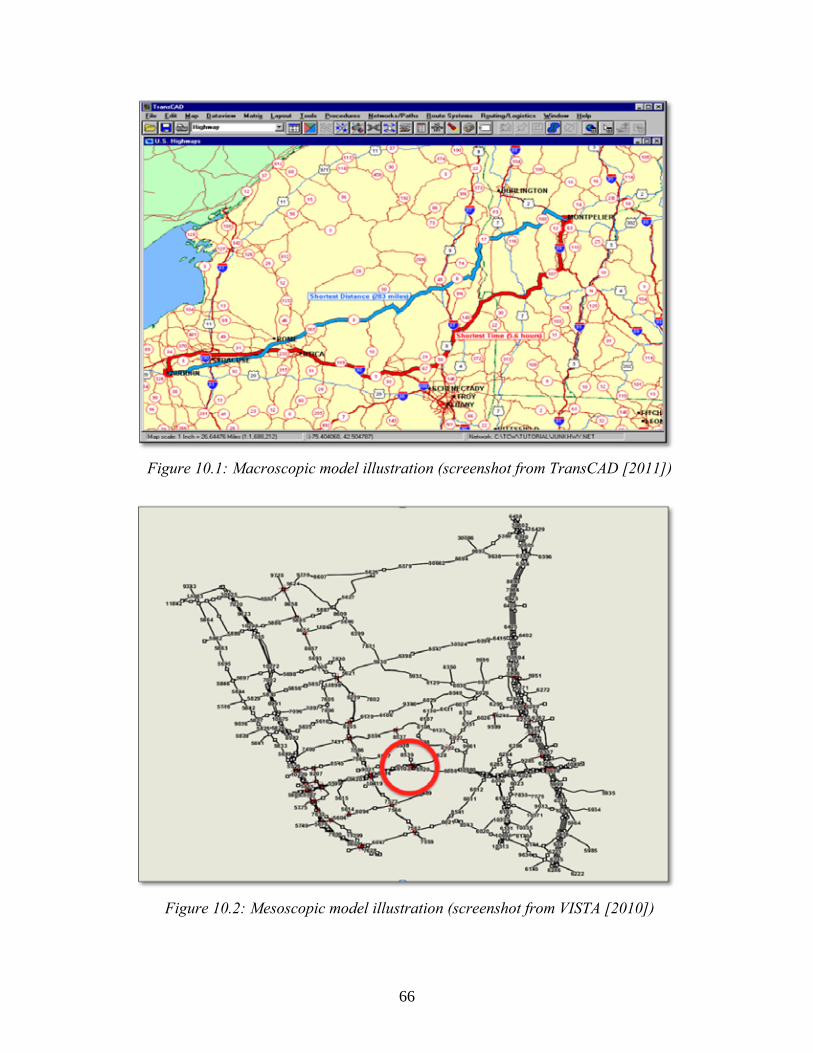
66
Figure 10.1: Macroscopic model illustration (screenshot from TransCAD [2011])
Figure 10.2: Mesoscopic model illustration (screenshot from VISTA [2010])
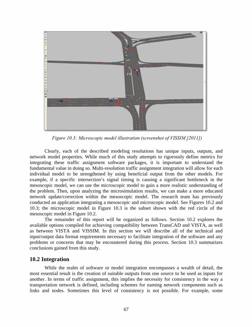
67
Figure 10.3: Microscopic model illustration (screenshot of VISSIM [2011])
Clearly, each of the described modeling resolutions has unique inputs, outputs, and network model properties. While much of this study attempts to rigorously define metrics for integrating these traffic assignment software packages, it is important to understand the fundamental value in doing so. Multi-resolution traffic assignment integration will allow for each individual model to be strengthened by using beneficial output from the other models. For example, if a specific intersection’s signal timing is causing a significant bottleneck in the mesoscopic model, we can use the microscopic model to gain a more realistic understanding of the problem. Then, upon analyzing the microsimulation results, we can make a more educated network update/correction within the mesoscopic model. The research team has previously conducted an application integrating a mesoscopic and microscopic model. See Figures 10.2 and 10.3; the microscopic model in Figure 10.3 is the subset shown with the red circle of the mesoscopic model in Figure 10.2.
The remainder of this report will be organized as follows. Section 10.2 explores the available options compiled for achieving compatibility between TransCAD and VISTA, as well as between VISTA and VISSIM. In this section we will describe all of the technical and input/output data format requirements necessary to facilitate integration of the software and any problems or concerns that may be encountered during this process. Section 10.3 summarizes conclusions gained from this study.
10.2 Integration
While the realm of software or model integration encompasses a wealth of detail, the most essential result is the creation of suitable outputs from one source to be used as inputs for another. In terms of traffic assignment, this implies the necessity for consistency in the way a transportation network is defined, including schemes for naming network components such as links and nodes. Sometimes this level of consistency is not possible. For example, some
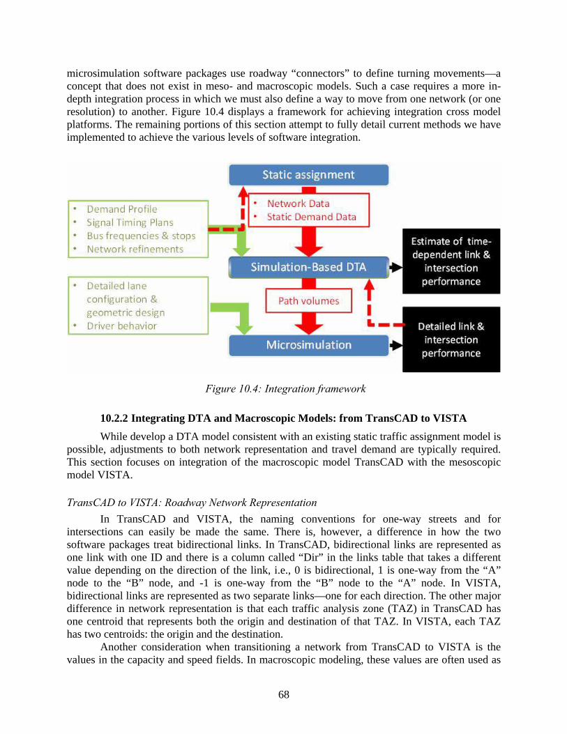
68
microsimulation software packages use roadway “connectors” to define turning movements—a concept that does not exist in meso- and macroscopic models. Such a case requires a more in- depth integration process in which we must also define a way to move from one network (or one resolution) to another. Figure 10.4 displays a framework for achieving integration cross model platforms. The remaining portions of this section attempt to fully detail current methods we have implemented to achieve the various levels of software integration.
Figure 10.4: Integration framework
10.2.2 Integrating DTA and Macroscopic Models: from TransCAD to VISTA
While develop a DTA model consistent with an existing static traffic assignment model is possible, adjustments to both network representation and travel demand are typically required. This section focuses on integration of the macroscopic model TransCAD with the mesoscopic model VISTA.
TransCAD to VISTA: Roadway Network Representation
In TransCAD and VISTA, the naming conventions for one-way streets and for intersections can easily be made the same. There is, however, a difference in how the two software packages treat bidirectional links. In TransCAD, bidirectional links are represented as one link with one ID and there is a column called “Dir” in the links table that takes a different value depending on the direction of the link, i.e., 0 is bidirectional, 1 is one-way from the “A” node to the “B” node, and -1 is one-way from the “B” node to the “A” node. In VISTA, bidirectional links are represented as two separate links—one for each direction. The other major difference in network representation is that each traffic analysis zone (TAZ) in TransCAD has one centroid that represents both the origin and destination of that TAZ. In VISTA, each TAZ has two centroids: the origin and the destination.
Another consideration when transitioning a network from TransCAD to VISTA is the values in the capacity and speed fields. In macroscopic modeling, these values are often used as
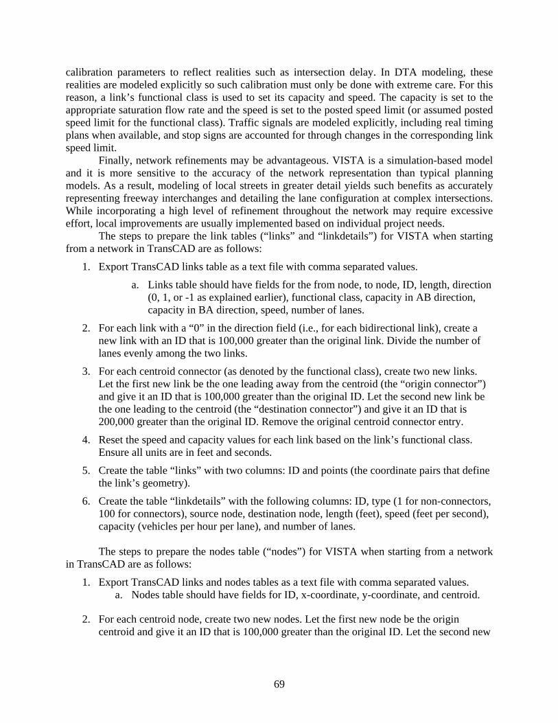
69
calibration parameters to reflect realities such as intersection delay. In DTA modeling, these realities are modeled explicitly so such calibration must only be done with extreme care. For this reason, a link’s functional class is used to set its capacity and speed. The capacity is set to the appropriate saturation flow rate and the speed is set to the posted speed limit (or assumed posted speed limit for the functional class). Traffic signals are modeled explicitly, including real timing plans when available, and stop signs are accounted for through changes in the corresponding link speed limit.
Finally, network refinements may be advantageous. VISTA is a simulation-based model and it is more sensitive to the accuracy of the network representation than typical planning models. As a result, modeling of local streets in greater detail yields such benefits as accurately representing freeway interchanges and detailing the lane configuration at complex intersections. While incorporating a high level of refinement throughout the network may require excessive effort, local improvements are usually implemented based on individual project needs.
The steps to prepare the link tables (“links” and “linkdetails”) for VISTA when starting from a network in TransCAD are as follows:
1. Export TransCAD links table as a text file with comma separated values.
a. Links table should have fields for the from node, to node, ID, length, direction (0, 1, or -1 as explained earlier), functional class, capacity in AB direction, capacity in BA direction, speed, number of lanes.
2. For each link with a “0” in the direction field (i.e., for each bidirectional link), create a new link with an ID that is 100,000 greater than the original link. Divide the number of lanes evenly among the two links.
3. For each centroid connector (as denoted by the functional class), create two new links. Let the first new link be the one leading away from the centroid (the “origin connector”) and give it an ID that is 100,000 greater than the original ID. Let the second new link be the one leading to the centroid (the “destination connector”) and give it an ID that is 200,000 greater than the original ID. Remove the original centroid connector entry.
4. Reset the speed and capacity values for each link based on the link’s functional class. Ensure all units are in feet and seconds.
5. Create the table “links” with two columns: ID and points (the coordinate pairs that define the link’s geometry).
6. Create the table “linkdetails” with the following columns: ID, type (1 for non-connectors, 100 for connectors), source node, destination node, length (feet), speed (feet per second), capacity (vehicles per hour per lane), and number of lanes. The steps to prepare the nodes table (“nodes”) for VISTA when starting from a network
in TransCAD are as follows:
1. Export TransCAD links and nodes tables as a text file with comma separated values. a. Nodes table should have fields for ID, x-coordinate, y-coordinate, and centroid.
2. For each centroid node, create two new nodes. Let the first new node be the origin centroid and give it an ID that is 100,000 greater than the original ID. Let the second new
70
node be the destination centroid and give it an ID that is 200,000 greater than the original ID. Remove the original centroid node entry.
3. The final table should have columns for ID, type (1 for non-centroids and 100 for centroids), x-coordinate, and y-coordinate.
TransCAD to VISTA: Demand Specification
The demand in static models is specified using a single O-D matrix, which represents the travel demand between TAZs throughout the considered assignment period. The former is consistent with the static modeling approach, which assumes that drivers will choose their routes based on the average conditions during the considered period. Dynamic models consider several assignment intervals within the assignment period. Both the travel demand and drivers’ route choices may vary across intervals. In order to allow for this flexibility, dynamic models require specifying a demand profile, describing how demand changes during the considered period. This profile can be uniform, implying a stable inflow of vehicles into the network throughout the analyzed hours, or have a specific shape based on available data. Another consequence of the use of simulation is that different vehicle types may be considered, each with specific properties.
The steps to prepare the demand table (“static_od”) for VISTA when starting from a network in TransCAD are as follows:
1. Export TransCAD demand matrix to a text file for each vehicle type that will be assigned to the network.
2. Update the centroid numbers to add 100,000 to each origin centroid ID and add 200,000 to each destination centroid ID.
3. Add a column to designate the vehicle type and give a unique number to each vehicle type.
4. Concatenate the demand tables into one table containing the demand for each type.
5. Add a column, “ID,” with a unique identifier for each row. The final table should have the following columns: ID, Type, Origin, Destination, Demand.
TransCAD to VISTA: Transit
In the context of VISTA, transit vehicles are represented using a specific vehicle class. These vehicles are assigned to fixed routes defined by the transit authority and are assigned stop locations and dwell times consistent with real bus stops.
Five tables are needed to define transit operations in VISTA:
1. Bus Route: Includes a unique ID per route and the corresponding name.
2. Bus Route Link: Lists the links defining each route, and the order in which they’re traversed. Links on which bus stops are present are also identified in this table.
3. Bus frequency: Defines the frequency at which buses depart, per route. The frequency may vary throughout the assignment period.
4. Bus period: Defines periods during which the frequency of one or more routes remains constant.
71
5. Bus stop: Assigns a unique ID to every physical bus stop, and includes a description if desired. Part of the information required to build the transit network may be exported from the
macroscopic model. The bus route link table may be obtained using GISDK macros, and the bus route table may be built based on the appropriate dataview in TransCAD. However, bus frequency information, and route-specific stops are typically not available in an easily transferable form from the macroscopic model. For bus stops, researchers have explored the use of Google’s GTFS (Generalized Transit Feed Spec) files. GTFS files may be processed using Excel and simple codes in C++.
TransCAD to VISTA: Other Needed Tables
VISTA inputs several other tables. Many of these are optional and problem-specific. The following two tables are required.
1. Vehicleclass: columns for ID for vehicle type, title of class, description of class.
2. Demand_profile: columns for ID (consecutive number for each time slice), weight (weight assigned to each time slice), starttime (seconds), duration (seconds).
a. The weights are applied to the demand in the static_od table to create the total demand in each time slice. Random number generation is then used within VISTA to assign vehicles to random times within their assigned time slice.
If diurnal factors are available from the static model, these can be used to inform the
demand profile. These factors are often useful for running DTA at a regional level. When running a subnetwork, the demand profile is created when the DTA regional path flows, which are inherently dynamic and have a profile over time, are extracted to create a subnetwork demand.
10.2.3 Integrating DTA and Microsimulation: from VISTA to VISSIM
VISTA model outputs consist of individual vehicle trajectories. From these we can compute a variety of time-dependent network performance measures, including intersection delay and link- or route-based travel time. However, due to the limitations of the traffic simulator implemented within the DTA framework, the resulting performance metrics do not explicitly take into account the friction introduced by weaving maneuvers or the impacts of lane widths and other intersection design characteristics. The latter may be relevant for some applications, including those concerning intersection improvements, freeway ramp design, and work-zone traffic control planning. In such cases, DTA outputs may be used to support the development of a microsimulation model, which can provide more refined performance metrics.
While microsimulation models representing present conditions may be built based on field data, the analysis of future year scenarios requires estimates of traffic volumes and turning movements, which can be obtained through DTA. Further, DTA outputs may be used to reduce the data collection needs for present year microsimulation analyses.
For this project, researchers developed a process to generate VISSIM (microsimulation) inputs from VISTA vehicle trajectory data. While the process details are specific to these software packages, the general method should be applicable to other packages such as CORSIM.
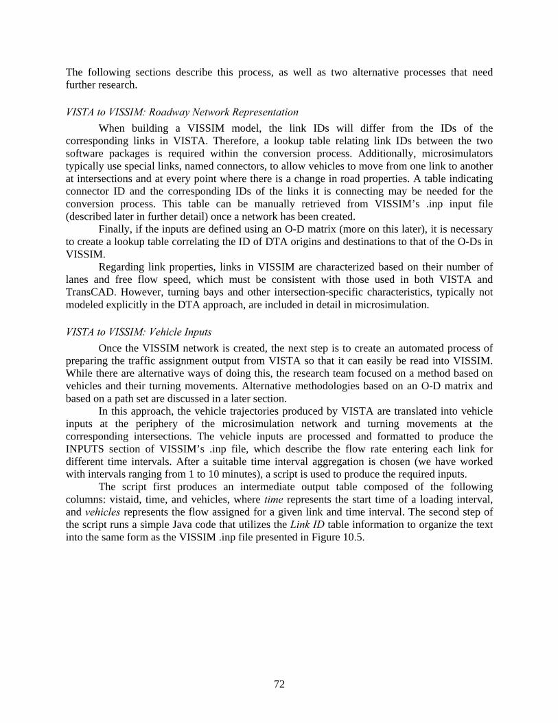
72
The following sections describe this process, as well as two alternative processes that need further research.
VISTA to VISSIM: Roadway Network Representation
When building a VISSIM model, the link IDs will differ from the IDs of the corresponding links in VISTA. Therefore, a lookup table relating link IDs between the two software packages is required within the conversion process. Additionally, microsimulators typically use special links, named connectors, to allow vehicles to move from one link to another at intersections and at every point where there is a change in road properties. A table indicating connector ID and the corresponding IDs of the links it is connecting may be needed for the conversion process. This table can be manually retrieved from VISSIM’s .inp input file (described later in further detail) once a network has been created.
Finally, if the inputs are defined using an O-D matrix (more on this later), it is necessary to create a lookup table correlating the ID of DTA origins and destinations to that of the O-Ds in VISSIM.
Regarding link properties, links in VISSIM are characterized based on their number of lanes and free flow speed, which must be consistent with those used in both VISTA and TransCAD. However, turning bays and other intersection-specific characteristics, typically not modeled explicitly in the DTA approach, are included in detail in microsimulation.
VISTA to VISSIM: Vehicle Inputs
Once the VISSIM network is created, the next step is to create an automated process of preparing the traffic assignment output from VISTA so that it can easily be read into VISSIM. While there are alternative ways of doing this, the research team focused on a method based on vehicles and their turning movements. Alternative methodologies based on an O-D matrix and based on a path set are discussed in a later section.
In this approach, the vehicle trajectories produced by VISTA are translated into vehicle inputs at the periphery of the microsimulation network and turning movements at the corresponding intersections. The vehicle inputs are processed and formatted to produce the INPUTS section of VISSIM’s .inp file, which describe the flow rate entering each link for different time intervals. After a suitable time interval aggregation is chosen (we have worked with intervals ranging from 1 to 10 minutes), a script is used to produce the required inputs.
The script first produces an intermediate output table composed of the following columns: vistaid, time, and vehicles, where time represents the start time of a loading interval, and vehicles represents the flow assigned for a given link and time interval. The second step of the script runs a simple Java code that utilizes the Link ID table information to organize the text into the same form as the VISSIM .inp file presented in Figure 10.5.
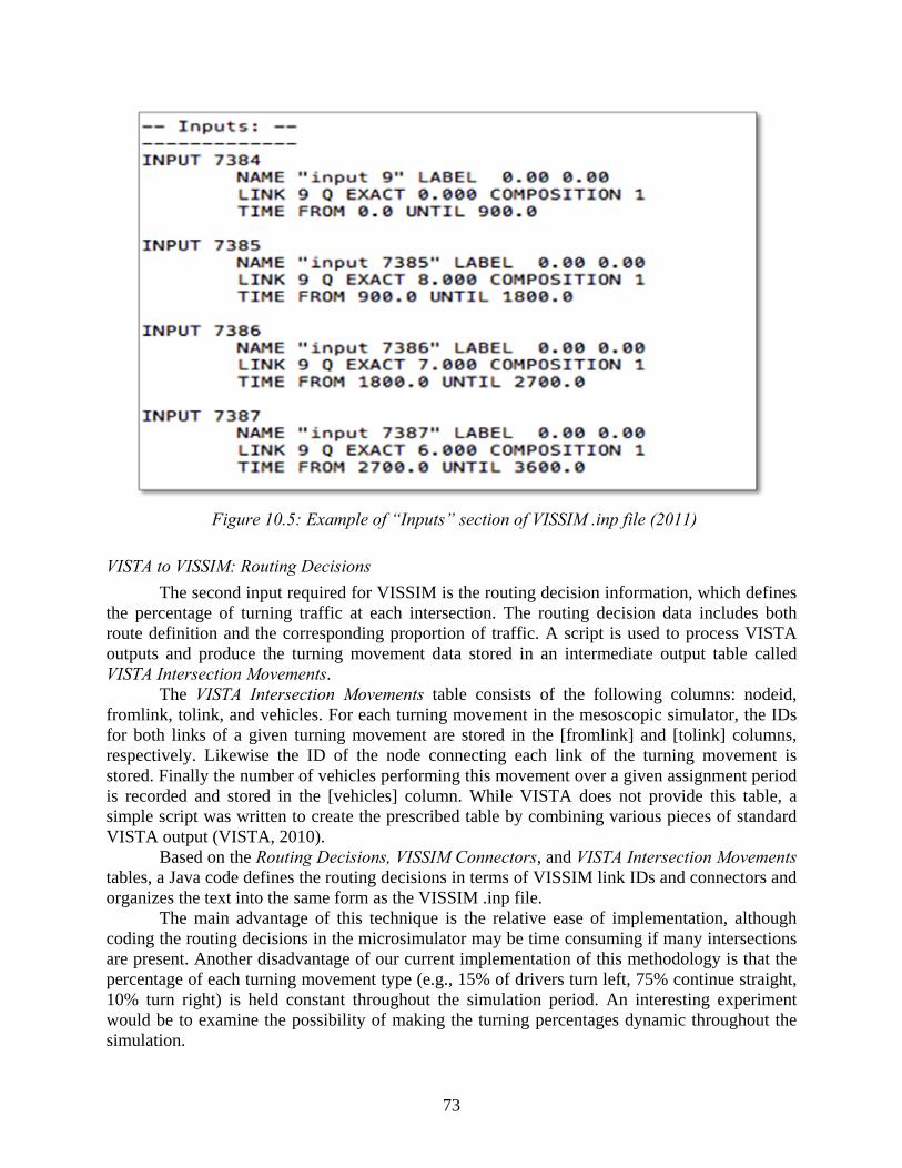
73
Figure 10.5: Example of “Inputs” section of VISSIM .inp file (2011)
VISTA to VISSIM: Routing Decisions
The second input required for VISSIM is the routing decision information, which defines the percentage of turning traffic at each intersection. The routing decision data includes both route definition and the corresponding proportion of traffic. A script is used to process VISTA outputs and produce the turning movement data stored in an intermediate output table called VISTA Intersection Movements.
The VISTA Intersection Movements table consists of the following columns: nodeid, fromlink, tolink, and vehicles. For each turning movement in the mesoscopic simulator, the IDs for both links of a given turning movement are stored in the [fromlink] and [tolink] columns, respectively. Likewise the ID of the node connecting each link of the turning movement is stored. Finally the number of vehicles performing this movement over a given assignment period is recorded and stored in the [vehicles] column. While VISTA does not provide this table, a simple script was written to create the prescribed table by combining various pieces of standard VISTA output (VISTA, 2010).
Based on the Routing Decisions, VISSIM Connectors, and VISTA Intersection Movements tables, a Java code defines the routing decisions in terms of VISSIM link IDs and connectors and organizes the text into the same form as the VISSIM .inp file.
The main advantage of this technique is the relative ease of implementation, although coding the routing decisions in the microsimulator may be time consuming if many intersections are present. Another disadvantage of our current implementation of this methodology is that the percentage of each turning movement type (e.g., 15% of drivers turn left, 75% continue straight, 10% turn right) is held constant throughout the simulation period. An interesting experiment would be to examine the possibility of making the turning percentages dynamic throughout the simulation.
74
VISTA to VISSIM: Alternative Methods for Transferring Vehicle Data
One alternative approach uses the vehicle trajectories produced by VISTA to generate an O-D matrix for the network area modeled in the microsimulator. The O-D ID table is then used within a script to format the VISTA O-D matrix for the considered subnetwork and generate the tables required by VISSIM. Given that no path information is provided, the microsimulator has to choose the routes for all assigned vehicles. To maintain consistency with the assignment software, this approach should only be applied when a corridor-type network is modeled in the micro simulator such that there is only one possible path connecting every specified O-D pair. This methodology requires minimum data processing but can only be applied to corridor analyses.
A second alternative approach directly feeds vehicle paths from VISTA into VISSIM, which makes it the most accurate way to integrate both models. The main challenge in implementing this technique is the lack of a one-to-one correspondence between VISTA links and VISSIM links/connectors. Further research is needed to develop methods to automatically convert VISTA paths into valid VISSIM paths.
10.3 Summary of Approach
This technical memorandum detailed methods for integrating macroscopic, mesoscopic, and microscopic models using the TransCAD, VISTA, and VISSIM software, respectively. The integration described herein goes from the less coarse to the more coarse models and the process typically involves adding detail. Further research is needed to determine whether fine-grained models can be used to inform coarse models and if so, how this should be done. While the details provided are particular to the three software packages mentioned, the methods described are more generally applicable to other packages such as the CORSIM microsimulation tool.
75
Chapter 11. Conclusions
This report described a research effort employing DTA modeling for improved bottleneck analysis at a regional scale. The study established the suitability of DTA models for such analysis. DTA models provide an ideal balance between the macroscopic and microscopic models for studying the impact of bottlenecks on regional traffic flow pattern at a sufficiently fine resolution that models the behavior of individual vehicles in response to bottlenecks and congestion.
After a review of relevant simulation-based DTA models, VISTA software was selected for performing this research study. VISTA meets the scope of this project, and its mesoscopic traffic flow model provides an ideal balance between traffic realism and computational efficiency. The research team has extensive experience with transportation modeling using VISTA, and the availability of its source code means that new features and updates can be added as needed. Its web-based interface provides flexibility and platform independence. VISTA models can be developed and their results demonstrated on any desktop PC.
In consultation with the Project Monitoring Committee, the researchers selected a test bed location that constituted MoPac Expressway in downtown Austin, including the Cesar Chavez Street (aka 1st Street) and 6th Street on-ramps. TxDOT made geometric changes to the MoPac Expressway near downtown Austin area in September 2010 to improve travel conditions for commuters traveling to and from downtown during peak periods. A bottleneck previously existed on this segment where the number of lanes was reduced from three to two. To capture any route switching due to the geometric reconfiguration, the test bed network was expanded to included downtown streets. The boundaries of the test bed were MoPac to IH 35 frontage and Cesar Chavez Street to 34th Street. To accurately capture queue formation and spillback effects on MoPac Expressway, the boundaries of MoPac were extended to Braker Lane in the north and Loop 360 in the south.
Various performance metrics at different levels of aggregation were selected to calibrate and validate a base case model and to evaluate the impact of geometric reconfiguration on travel condition. DTA produces several performance metrics that can be broadly classified in two categories: (1) volume-based measures, such as throughput, volume-to-capacity ratio, density, route choice, etc., and (2) travel time-based measures, such as travel time, delay, speed, etc. A base case DTA model was satisfactorily calibrated and validated using flow and travel time measures, respectively. This step produced a robust base case model for performing subsequent analyses, and for creating an “after” case model by making appropriate modifications in the network.
The geometric changes made by TxDOT to the MoPac Expressway near downtown led to a small improvement in northbound MoPac travel time during the latter half of the 4:00–6:00 p.m. peak period. The new lane configuration also drew more northbound vehicles to MoPac through the Cesar Chavez/6th Street approach and lead to a small increase in travel time on this ramp. Vehicular counts on the Enfield Road on-ramp did not change significantly. There were no major shifts in travel patterns of the commuters leaving downtown in the evening. Overall, no major route-switching behavior was observed in the network.
The research team supplemented the core bottleneck analysis using DTA with additional tools to help transportation planning decision-makers. A simplified Analytical Hierarchy Process was developed to rank potential improvement projects as part of the decision-making framework. An example cost-benefit analysis using reasonable assumptions demonstrated the benefit of the
76
geometric reconfiguration, primarily due to decreased crash likelihood. Guidelines were provided to incorporate DTA into the traditional four-step planning model at the regional and sub-network levels. This is an ongoing research effort and an open research problem with great potential because more transportation agencies are using DTA or showing inclination to do so in their planning process and traffic operations.
The adoption of DTA by transportation agencies also presents new challenges in integratating DTA with existing traffic models currently in use. In order to take full advantage of DTA, traffic analysts will need to integrate a variety of tools with different capabilities operating at varying degree of resolutions, and establish standardized interfaces between such software packages. The final sections of the report are dedicated to providing guidelines for such integration by drawing a sample software from each degree of resolution (macroscopic, mesoscopic, and microscopic).
77
References
Agrawal, B. B., and S. T. Waller, et al. (2002). "Modeling approach for transit signal preemption." Transportation Research Record: Journal of the Transportation Research Board. 1791: 13-20.
Ben-Akiva, M., Palma, A.D., and Kanaroglou, P. (1986). “Dynamic model of peak period traffic with elastic arrival rates.” Transportation Science, Vol.20 (3), pp.164-181.
Bhat, C.R. and R. Sardesai. “The Impact of Stop-Making and Travel Time Reliability on Commute Mode Choice.” Transportation Research Part B, Vol. 40, No. 9, 2006, pp. 709 – 730.
Bhat, C.R., N. Eluru, D.Y. Lin, and S.T. Waller. “Integration of Activity-Based Modeling and Dynamic Traffic Assignment.” Transportation Research Record: Journal of the Transportation Research Board, No. 2076, Transportation Research Board of the National Academies, Washington, D.C., 2008, pp. 52–61.
Birge, J. R., and J. K. Ho (1993). "Optimal flows in stochastic dynamic networks with congestion." Operations Research, 41(1): 203-216.
Bottom, J., Y. Chiu, et al. (2011). Dynamic Traffic Assignment: A Primer, Transportation Research Circular Number E-C153, Transportation Research Board, Washington, D.C. Available online at http://onlinepubs.trb.org/onlinepubs/circulars/ec153.pdf
Boyce, D. E., B. Ran, et al. (1995). "Solving an instantaneous dynamic user-optimal route choice model." Transportation Science, 29(2): 128-142.
Braess, D., “Über ein Paradoxon aus der Verkehrsplanung,” Unternehmensforschung 12, pp. 258-268, 1968.
Brown, C.M. “Dynamic Traffic Assignment and Mesoscopic Simulation with Cube Avenue.”Presented at the SEFL FSUTMS User Group July 8 Meeting. www.fsutmsonline.net%2Fimages%2Fuploads%2Fsoutheastfloridafsutms%2FDTA_Meso-Citilabs.pdf Accessed August 2012.
Bureau of Public Roads. Traffic Assignment Manual. Office of Planning, Urban Planning Division, Washington, D.C., 1964.
Cambridge Systematics, Inc. NCHRP Report 446: A Guidebook for Performance-Based Transportation Planning. TRB, National Research Council, Washington, D.C., 2001.
Cambridge Systematics, Inc. Report prepared for Austin-San Antonio Intermunicipal Commuter Rail District. Final Report: Financial & Economic Benefits Study. Austin, TX. March 2007.
Carey, M. (1986). "A constraint qualification for a dynamic traffic assignment model." Transportation Science, 20(1): 55.
78
Carey, M. (1987). "Optimal time-varying flows on congested networks." Operations Research 35(1): 58-69.
Carey, M. (1992). "Nonconvexity of the dynamic traffic assignment problem." Transportation Research Part B: Methodological, 26(2): 127-133.
Carey, M. and E. Subrahmanian (2000). "An approach to modelling time-varying flows on congested networks." Transportation Research Part B: Methodological, 34(3): 157-183.
Cassidy, M.J., and Bertini, R.L. (1999). “Some traffic features at freeway bottlenecks.” Transportation Research Part B, Vol. 33(1), pp. 25-42.
Chang, E. and A. Ziliaskopoulos (2007). "A simulation-based dynamic intermodal network equilibrium algorithm." Network Science, Nonlinear Science and Infrastructure Systems: 201-222.
Chen, M., and M.N. Sweet. “Does Regional Travel Time Unreliability Influence Mode Choice?” Transportation, Vol. 38, 2011, pp. 625 – 642.
Chiu, Y.-C., Zhou, L., and Song, H. (2010). “Development and calibration of the Anisotropic Mesoscopic Simulation model for uninterrupted flow facilities.” Transportation Research Part B: Methodological, Elsevier Ltd, 44(1), 152-174.
Chiu, Y.C., R. Tung, and Z. Wang. “Integration of Dynamic Traffic Assignment in a Four-Step Model Framework – A Deployment Case Study in Seattle Model.” Presented at the 3rd Conference on Innovations in Travel Modeling, 2010.
Cooner, S.A., and Ranft, S.E., and Walters, C.H.. “Reconsidering Freeway Bottlenecks: Case Studies of Bottleneck Removal Projects in Texas.” Transportation Research Record: Journal of the Transportation Research Board, No. 1925, Transportation Research Board of the National Academies, Washington, D.C., 2005, pp. 66–75.
Daganzo, C. F. (1994). "The cell transmission model: A dynamic representation of highway traffic consistent with the hydrodynamic theory." Transportation Research Part B: Methodological, 28(4): 269-287.
Daganzo, C. F. (1995). "The cell transmission model, part II: Network traffic." Transportation Research Part B: Methodological, 29(2): 79-93.
FHWA. (2007). "Traffic Bottlenecks." from http://ops.fhwa.dot.gov/bn/index.htm.
FHWA (2010) Traffic Analysis Toolbox Volume X: Localized Bottleneck Congestion Analysis. Publication No. FHWA-HOP-09-042, March 2010.
Florian, M., Mahut. M., and Tremblay, N. (2008). “Application of a simulation-based dynamic traffic assignment model.” European Journal of Operations Research. 189(3),1381–1392.
79
Gentile, G., L. Meschini, et al. (2007). "Spillback congestion in dynamic traffic assignment: A macroscopic flow model with time-varying bottlenecks." Transportation Research Part B: Methodological, 41(10): 1114-1138.
Holyoak, Nocholas and Branko Stazic. “Benefits of Linking Macro-Demand Forecasting Models and Microsimulations Models.” ITE Journal, Voume 79, Issue 10 (2009): pp 30-39.
Institute of Transportation Engineers. Trip Generation: An ITE Information Report (8th Edition). Institute of Transportation Engineers, Washington, D.C., 2008.
Janson, B. (1991). "Convergent algorithm for dynamic traffic assignment." Transportation Research Record 1328: 69-80.
Janson, B. N. (1991). "Dynamic traffic assignment for urban road networks." Transportation Research Part B: Methodological, 25(2-3): 143-161.
Juran, I., Prashker, J.N., Bekhor, S., and I. Ishai (2009). “A dynamic traffic assignment model for the assessment of moving bottlenecks.” Transportation Research Part C, Vol. 17(3), pp. 240-258.
Kerner, B.S. (2002). “Empirical macroscopic features of spatial-temporal traffic patterns at highway bottlenecks.” Physical Review E, Vol. 65(4).
Kerner, B.S., and Klenov, S.L. (2003). “Microscopic theory of spatial-temporal congested traffic patterns at highway bottlenecks.” Physical Review E, Vol. 68(3).
Lee, S., (1996). “A cell transmission based assignment-simulation model for integrated freeway/ surface street systems.” Master Thesis, Ohio State University.
Lighthill, M. J. and G. B. Whitham (1955). "On kinematic waves. II. A theory of traffic flow on long crowded roads." Proceedings of the Royal Society of London. Series A, Mathematical and Physical Sciences 229(1178): 317-345.
Mahut, M., Florian, M., Tremblay, N., Campbell, M., Patman, D., and Mcdaniel, Z. K. (2004.). “Calibration and Application of a Simulation-Based Dynamic Traffic Assignment Model.” Transportation Research Record, 101-111.
Merchant, D. K. and G. L. Nemhauser (1978). "A model and an algorithm for the dynamic traffic assignment problems." Transportation Science, 12(3): 183-199.
Merchant, D. K. and G. L. Nemhauser (1978). "Optimality conditions for a dynamic traffic assignment model." Transportation Science, 12(3): 200-207.
National Institute of Standards and Technology. Engineering Statistics Handbook. National Institute of Standards and Technology, Technology Administration, U.S. Department of Commerce, Washington, D.C., 2003.
Peeta, S. and A. Ziliaskopoulos (2001). "Foundations of dynamic traffic assignment: the past, the present and the future." Networks and Spatial Economics 1(3): 233-265.
80
“Proposed Lane Reconfiguration along Loop 1 North of Lady Bird Lake,” Texas Transportation Institute, April 16, 2010.
Ran, B., D. E. Boyce, et al. (1993). "A new class of instantaneous dynamic user-optimal traffic assignment models." Operations Research, 41(1): 192-202.
Ran, B. and T. Shimazaki (1989). Dynamic user equilibrium traffic assignment for congested transportation networks. Fifth World Conference on Transport Research, Yokohama, Japan.
Ran, B. and T. Shimazaki (1989). A general model and algorithm for the dynamic traffic assignment problems. Fifth World Conference on Transport Research, Yokohama, Japan.
Saaty, T.L., and Vargas, L.G.. “The Logic of Priorities, Applications in Business, Energy, Health and Transportation.” Boston: Kluwer-Nijhoff Publishing, 1982. Print.
Shaw, T. (2003). “Performance measures of operational effectiveness for highway segments and systems.” NCHRP synthesis of Highway Practice Issue No. 311, Transportation Research Record.
TransCAD 5.0, Caliper Corporation, 2011.
VISSIM 5.40-01 – User Manual. PTV Karlsruhe, Germany, 2011.
VISTA User Guide. Vista Transport Group, Inc., 2010.
Waller, S.T., and A. Ziliaskopoulos (2006). "A combinatorial user optimal dynamic traffic assignment algorithm." Annals of Operations Research, 144(1): 249-261.
Waller, S. T. and A. K. Ziliaskopoulos (2002). "On the online shortest path problem with limited arc cost dependencies." Networks, 40(4): 216-227.
Wardell, W. and A. Ziliaskopoulos. (2000). "An intermodal optimum path algorithm for multimodal networks with dynamic arc travel times and switching delays." European Journal of Operational Research, 125(3): 486-502.
Zhao, X., and Gao, Z. (2006). “A control method for congested traffic induced by bottlenecks in the coupled map car-following model.” Physica A: Statistical Mechanics and its Applications, Vol. 366, pp. 513-522.
Ziliaskopoulos, A. (1994). Optimum path algorithms on multidimensional networks: Analysis, design, implementation and computational experience, University of Texas at Austin. Ph.D.
Ziliaskopoulos, A. K. (2000). "A linear programming model for the single destination system optimum dynamic traffic assignment problem." Transportation Science, 34(1): 37-49.
81
Ziliaskopoulos, A. K. and H. S. Mahmassani (1993). "Time-dependent, shortest-path algorithm for real-time intelligent vehicle highway system applications." Transportation Research Record 1408: 94–100.
Ziliaskopoulos, A. K. and S. T. Waller (2000). "An Internet-based geographic information system that integrates data, models and users for transportation applications." Transportation Research Part C: Emerging Technologies, 8(1-6): 427-444.
Ziliaskopoulos, A. K., S. T. Waller, et al. (2004). "Large-scale dynamic traffic assignment: implementation issues and computational analysis." Journal of Transportation Engineering, 130(5): 585-593.