investigate the appropriateness of several tests of

DOCUMENT RESUME

ED 067 401 TM 001 796

AUTHOR Sween, Joyce; Campbell, Donald T.TITLE A Study of the Effect of Proximally Autocorrelated

Error on Tests of Significance for the InterruptedTime Series Quasi-Experimental Design.

INSTITUTION Northwestern Univ., Evanston, Ill.SPONS AGENCY Office of Education (DREW), Washington, D.C.

Educational Media Branch.REPORT NO Pro j-C998PUB DATE Aug 65CONTRACT 4EC-3-20-001NOTE 43p.

EDRS PRICE MF-$0.65 HC-$3.29DESCRIPTORS *Correlation; *Data Analysis; *Mathematical Models;

*Measurement Techniques; Statistics; Tests; *Tests ofSignificance

IDENTIFIERS Double Extrapolation Technique; Mood Test; Walker LevTest 3

ABSTRACTThe primary purpose of the present study was to

investigate the appropriateness of several tests of significance foruse with interrupted time series data. The second purpose was todetermine what effect the violation of the assumption of uncorrelatederror would have on the three tests of significance. The three testswere the Mood test, Walker-Lev Test 3, and Double ExtrapolationTechnique. The procedure was basically that of generating a largenumber of time series having specified characteristics and performingthe tests of significance on each generated time series. The resultsof the study indicated that the three tests of significance areappropriate for use on data of interrupted time series form. Tablesand figures illustrate the text. (Author/DB)

U.S. DEPARTMENT OF HEALTH.EDUCATION 8 WELFAREOFFICE OF EDUCATION

THIS DOCUMENT HAS BEEN REPRO.OUCED EXACTLY AS RECEIVED FROM

4THE PERSON OR ORGANIZATION ORIG-e- INATING IT POINTS OF VIEW OR OPIN

C) IONS STATED 00 NOT NECESSARILYREPRESENT OFFICIAL OFFICE OF EDUCATION POSITION OR POLICY

A STUDY OF THE EFFECT OF PROXIMALLY AUTOCORRELATELD ERRORON TESTS OF SIGNIFICANCE FOR THE INTERRUPTED

TIME SERIES QUASIEXPFILImENIAL DESIGN*

Joyce Sween and Donald T. Campbell

August 1965

Northwestern university

*Supported by Project C998, Contract 3-20-001, Educational MediaBranch, Office of Education, U.S. Department of Health, Education, andWelfare, under provisions of Title VII of the National Defense EducationAct.

FILMED FROM BEST AVAILABLE COPY

A Study of the Effect of Proximally Autocorrelated Error

on Teats of Significance for the Interrupted

Time-Series Quasi-Experimental Design

Joyce Sween and Donald T. Campbell

Northwestern University

The time series experiment has long been a common research design in

the biological and physical sciences. However, with psychological and soci-

ological data certain problems of analysis and interpretation occur when the

interrupted time series design is employed (Campbell, 1963; Campbell &

Stanley, 1962; Holtzman, 1963).

One of the problems which is of particular concern to the social

scientist (for whom the magnitude and clarity of effects is not always as

clear-cut as in the biological and physical sciences) is testing for the

significance of the change, X. It is desired to have some statistical test

of significance that would distinguish the effect of an intervening event or

experimental variable from purely random fluctuation. Although there are no

tests of significance that are completely suitable to the time series,situa-

tion, several possibilities for such a test do exist and merit consideration

(Campbell, 1963; Campbell & Stanley, 1962).

Another problem of fundamental concern to the social scientist is the

possibility of sequential dependency in successive observations of the time

series. Measurements made at time points which are closer together may be

more strongly related than measurements made farther apart in time. Statis-

tical models on which the tests of significance are based generally assume

that the observed values exhibit independent error. Thus, the significant

1

2

autocorrelation which exists when a given observation is dependent upon the

observations prOcedime it violates the assumption of independence in these

tests. Although this circumstance does not prevent estimation (by least

square methods) of the regression tocificients which the various tests of

significance use, as classical formulae for the mean errors of the estimated

coefficients are in actuality no longer valid. When successive observations

through time are correlated, perhaps, to a lag of several points, use of

existing tests of significance may be inappropriate.

The primary purpose of the present study was to investigate the appro-

priateness of several tests of significance for use with interrupted time

series data. The three main tests were those described by Mood (1950, pp.

297-298; pp. 350-358) and Walker and Lev (1953, pp. 390-395; pp. 399-400).

The interrupted time series experiment as considered in the present

study consists of a finite sequence of observations which are real-valued

measurements of some individual or group obtained at n successive eg_ually

spaced points in time. An experimental change is then introduced or a major

change of conditions occurs at some point in the time series. In the pres-

ent study, the experimental change or treatment is assumed to occur midway

between two consecutive measurements. It can be diagrammed as follows:

Interrupted Time Series DesigB

Observation at time t1:

Time:

Yl Y2 ' Ym Ym+1 Ym+2

t1 t2 ... tm itm+1 tm+2

experimentalchange

. . .n

to

The yi are the measurements recorded as time ti. The values yi(i /11 1,2, ...m)

obtained prior to the treatment are referred to as pre - change values. The

3

3

values yi (i m 1, m 2,...n) obtained after the treatment are post-

claws values. If the treatment has produced an effect, a discontinuity of

measurements is recorded in the time series. The statistical tests of sig-

nificance which were investigated in the present study as possible techniques

for distinguishing such a treatment effect from purely random fluctuation

are described in detail below:

(a) Mood Test. This is a t teat (Mood, 1950, pp. 297-298) for the sig-

nificance of the first post-change observation from a value predicted by a

linear fit of the pre-change observations. The fomala for t is

( Y. 7 ) /644.

A m 75a /6'1 4)6AThe estimate, yo , of the first post-change value is obtained from the pre-

change regression estimates .1,

(11164 44

t-L.,

A

Olk

where m a. number pre-change points

E hntVot

tz,The difference between the estimated value and the obtained first post-change

value, x, , is used in the t teat. Since and anInv 2(t; -i)aop,a urn,/,, AA

estimate, se , of 6'4 is given by evi 0#-or...) , the computation

formula for the t test of the difference between the obtained and predicted

post-change point is given by

k- ;%idi

iffriti .f. (1-6-E ).?' i t(YL"--:4-15i-zr( rn

ovi-a.'I4

The denominator is the standard error of the difference for t. The df for

t is (m-2). The significance of the obtained t is evaluated by reference to

a standard t table.

(b) Walker-Lev Tests. Walker and Lev (1953, pp. 390-395) provide the

following tests of significance. These tests are useful in determining

whether differences exist between the regression equations for pre- and post-

change groups.

Test One.

This is a test of the hypothesis of common slope. The F ratio is

F-S.

. (N-4)

where Si sum of squares of the common within groups regressionestimates from the separate group regression estimatesA

Liy ]*j al

S2 sum of squares of the obtained occasion values from theseparate group regression estimates

> [ x 614 t.01.2.Jz

N s total number of occasions in time seriesi =1, 2 11=prechange group; 2= postchange group]

given by

j 1, 2, ...Nt

Formulas for the common within groups slope and intercept are

EMI ryt.4Jc. T,A)

t7(1,,,. _ BW 2-z

Formulas for the separate4Aroup slopes and intercepts are

jr. IA

=

The computational formulae for the numerator and denominator sum of squares

for the F ratio are

5.=CTI*ta

where

z C )(Yu, eTT,:

40:

N,

C. TTe Zizja4=0

GY>:, =2_ x;'

=

c7-7-44=

Y>14 d1

CT re

f./

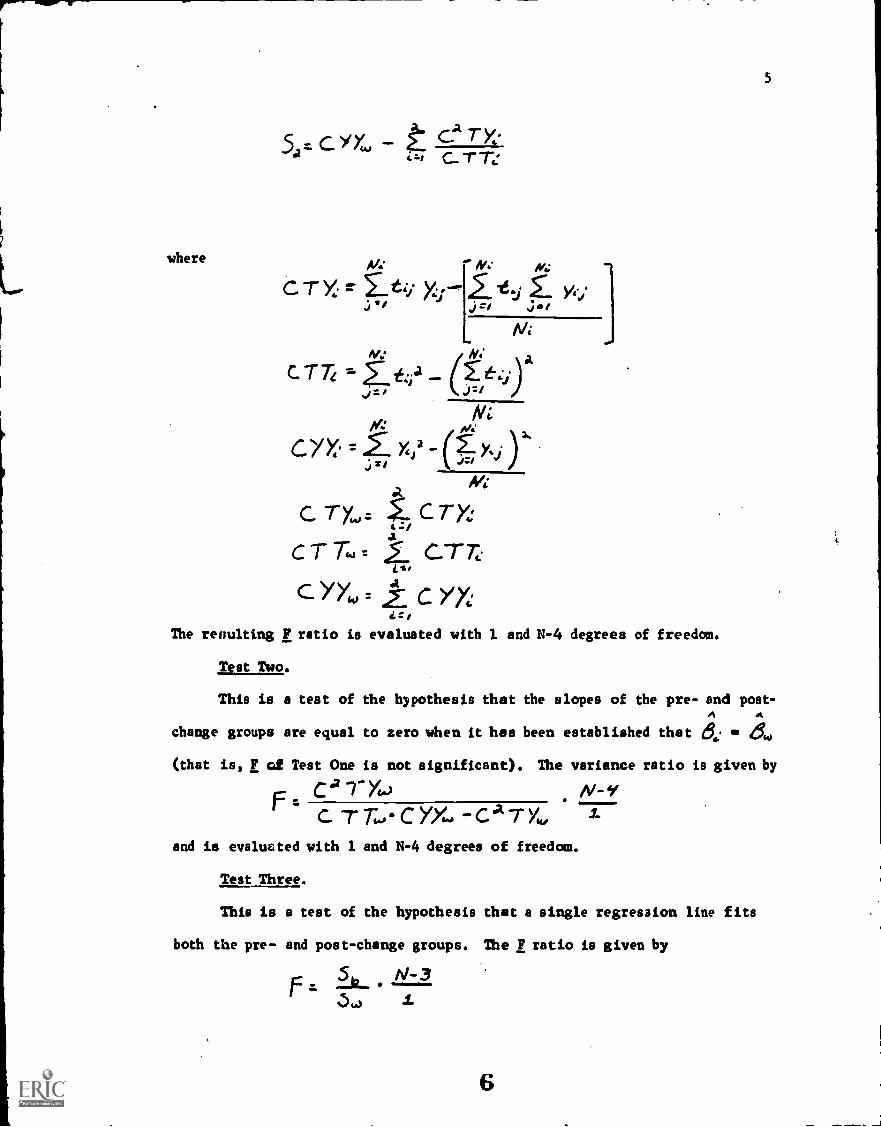
5

The renulting F ratio is evaluated with 1 and N-4 degrees of freedom.

Test Two.

This is a test of the hypothesis that the slopes of the pre- and post-A A

change groups are equal to zero when it has been established that 45,.. - Bw

(that is, F of Test One is not significant). The variance ratio is given by

C' 77t.)F C Trt.JCYX,and is evaluated with 1 and N-4 degrees of freedom.

Test Three.

This is a test of the hypothesis

both the pre- and post-change groups.

F . N-s3

N-

that a single regression line fits

The F ratio is given by

6

where Sb

6

sum of squares of common within groups regression estimates fromthe total series regression estimates

Sy sum of squares of obtained ;ma s ion values from the common withingroups regression estimates

A Aft: ACC

IA)jFormulas for the total series slope and intercept are

C. YT

C -r Tr

;(T.' i-8-rF

The computational formulae for the numerator and denominator sum of squares

for the F ratio are

= C Y * CITY& 7 YTCTTw CTTT

where

Sw ir So st

A Ni

CT YT Z

Ni A N4.

a A

Ygli) N

A N4,*

C T TT _pit, ( t1)/N1

CYY,atCYYT-C>'n,

'7

7

The resulting F ratio is evaluated with 1 and N-3 degrees of freedom.

(c) "Double Extrapolation" Tee/m.1mm. This test is concerned with the

significance of the difference between two separate regression estimates of

the y-value for time to which lies midway between the last pre-change point

and the first post-change point. Reference to the Interrupted Time Series

Design diagramed on page 2 will indicate that this point lies midway

between to and too.. Assuming that the points are equally spaced in time,

to is equal to tig..5 4,

The first regression estimate for yo is obtained from the pre-change

values; the second regression estimate for yo, from the post-change values.

The formulas for the two regression estimates aretie

64 'et/ t'vg YO/M:J=1

Jzi

A

where i se 1,2 [1 on prechange group; 2 as postchenge group]number occasions in group i1,2,...Ni

Thus , the two estimates for yo ere given by Y.:A

between these two estimates can be evaluated by the t-ratio t

The difference

190,- 90J

and its significance determined by reference to a t table with N1 N2 4

degrees of freedom. The stsudard error of the difference for j depends upon

the variability of the pre- and post-change values, Ni and N2, the relation

between t and y, and the distance of to from t1 and t2. The formula for S.,

is given in Walker and Lev (p. 400) as

(cyye-c-a---;:4 1[6, *A (t. 1

t a/

/V, t /VA i I

c iii C T T:

where

cTT =

cry,

Wd

ZA4 6.-jz (4, iv )71,k 1

L /Ytj ytsd

Jzi

The second purpose of the present study w;a to determine what effect

8

the violation of the assumption of uncorrelAed error would have on the

three tests of significance. Do the tests become inappropriate when there

is positive autocorrelation between points?

The scientist usually does not have knowledge of the degree of sequen-

tial dependency which exists in a given time series. The first serial cor-

relation coefficient (of lag one) is used to determine whether the observa-

tions of a given time series can be regarded as consisting of independent

error only (measures not correlated). The serial correlation coefficient

tests the hypothesis that the order of dependence in the time series is zero

against the alternative that it is one. Serial correlation coefficients of

lags higher than one can also be considered. (If the serial correlation is

that of a variable with itself, it may be referred to as an auto-correlation

coefficient.)

A serial correlation coefficient of lag one, r1, is obtained by pair-

ing observations one time unit apart; that is, the first observation is

paired with the secon4, the second with the third, etc., throughout the

9

9

entire time series until the last observation is reached. The product-moment

correlation is computed using the resulting pairs of observations. In a

similar manner, the second serial correlation coefficient, r2i is obtained

by pairing successive observations two time units apart and rm is obtained

by pairing observations si units apart. The basic formula for ra is givenel

below: .n w

Y;14 -(1 `Ata

/ I=

where N a= total number of occasions in the time seriesn N-a

1,2,...n

The model of autocorrelation used in the present study is basically

one of proximity, namely, it was assumed that measurements made closer

together in time would be more strongly related than measurements made fur-

ther apart in time. This means that in instances where a significant auto-

correlation ra exists, increasingly larger autocorrelations should exist for

ra_1, ra_2, .... and r1, respectively.

Since the slope of the line contributes to serial dependency between

points, interest in the present study is in the autocorrelations of depart-

ures from the line of beat fSt for the total series. However, because true

effects increase proximal autocorrelation, differences from the separate

pre- and post-change regression lines give better estimates of existing auto-

correlations in instances of true effects. So as not to penalise true

effects in the data version of the program (a computer program which performs

the tests of significance on input data of interrupted time series form is

10

10

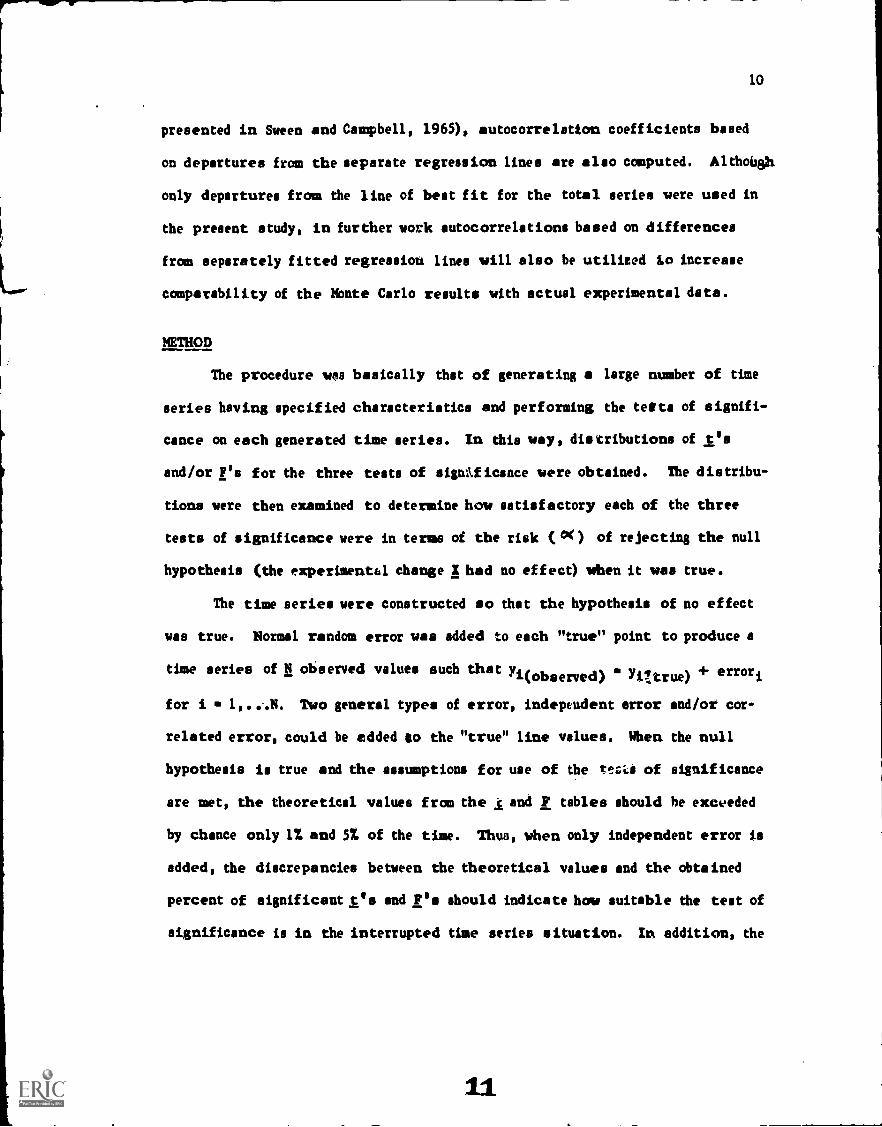
presented in Sween and Campbell, 1965), autocorrelation coefficients based

on departures from the separate regression lines are also computed. Although

only departures from the line of best fit for the total series were used in

the present study, in further work autocorrelations based on differences

from separately fitted regression lines will also be utilized is increase

comparability of the Monte Carlo results with actual experimental data.

METHOD

The procedure was basically that of generating a large number of time

series having specified characteristics and performing the tests of signifi-

cance on each generated time series. In this way, distributions of isand/or F's for the three tests of sigmlficance were obtained. The distribu-

tions were then examined to determine how satisfactory each of the three

tests of significance were in terms of the risk (*() of rejecting the null

hypothesis (the experimental change N had no effect) when it was true.

The time series were constructed so that the hypothesis of no effect

was true. Normal random error was added to each "true" point to produce a

time series of N observed values such that vwi(observed) yiltrue) + errori

for i 1,....N. Two general types of error, indeptudent error and/or cor-

related error, could be added so the "true" line values. When the null

hypothesis is true and the assumptions for use of the te;Li of significance

are met, the theoretical values from the and F tables should he exceeded

by chance only 1% and 5% of the time. Thus, when only independent error is

added, the discrepancies between the theoretical values and the obtained

percent of significant is and F's should indicate haw suitable the test of

significance is in the interrupted time series situation. In addition, the

ii

11

obtained percentage of is and F's which exceed the theoretical values when

sequential dependency between points is built in should indicate how the

violation of the assumption of independence of error may further restrict

the usefulness of the tests.

Each generated time series could be varied with respect to (a) the

number of pre- and post-change occasion values,(b) the slope of the "true"

line, (c) the degree of autocorrelation between points, and (d) the total

error variance about the true line values. In the present study the follow-

ing combinations of pre- and post-change occasion values, "true" line slopes,

autocorrelated error, and error variance were used:

(a) Pre- and post- change sample sizes of 10, 20, and 100 were used toyield time series with the following number of total occasion values:

Total Occasions, N 20 (pre 10; post 10)Total Occasions, N 40 (pre - 20; poet a 20)Total Occasions, N 2W.;'(pre 100; post -100)

In the presentation of the results these three conditions of sampl-ing are referred to in terms of the total occasions in the series asN 20, N 40, and.N 200. The degrees of freedom and criticalvalues for the Mood test of significance are, however, based onlyupon the pre-change points of 10, 20, and 100. For the Walker-LevTest 3 and Double Extrapolation Technique the total series points of20, 40, and 200 are used.

(b) The slope of the true line was specified as 0..0, 1.0, and 20.0.

(c) The degree of autocorrelated error was specified se zero (independ-ent error only), one, two, and three (correlated error for measure-ments one, two, and three time lags apart).

(d) Total error variance about the true line was specified at 1.00 and5.00 and normal random error was drawn from Gaussian distributionsof zero mean and appropriate standard deviations to yield equalerror variance about the true line for all degrees of autocorrelatederror.

For the total error variance specified as 1.00, the standard devia-tions of the normal distributions from which the normal randomerrors were drawn would be

12

1.00 (unique error only).58 (unique plus error of lag 1).50 (unique plus error of lag 27.45 (unique plus error of lag 3)

For a total error variance specified as 5.00, the standard deviationsof the norms/ distributions from which the normal random errors weredrawn would be

2.24 (unique error only)1.29 (unique plus error of lag 1)1.12 (unique plus error of lag 2)1.00 (unique plus error of lag 3)

One thousand sets of time series were generated for each type of auto-

correlated error in various combinations with the options of sample size,

true line slope, and total error variance listed in a, b, and d above. The

following tests of significance were performed on each of the 1000 sets of

generated data: Mood test, Walker-Lev Test 3, Double Extrapolation tech-

nique. .The Walker -Lev Tests 1 and 2 and a test proposed by Clayton and

described by Campbell (1963, p. 225) were performed on a smaller sample of

100 sets of generated time series.]i

For each test of significance, the percent of I's or F's which exceeded

the theoretical 1% and 57. values was determined. The complete sequence of

operations was performed internally on the IBM 709 computer proteviprogram-

med to perform the necessary operations. The basic steps in the computation

procedures are summarized below:

(1) The "true" line pre- and post-X occasion values were determined onthe basis of desired slope. Normal random errors yielding specifiedautocorrelation were added to the "true" line points to form the setof time series data. (A binary subprogram from the Vogelback com-puting center (NU-0044) was used for the generation of normal randomnumbers. The mean of the Gaussian distribution approximates zero;the standard deviation was specified as described in (d) above).The program generated 1000 sets of time series for each type oferror fluctuation specified.

(2) F and t values for the Mood, Walker-Lev 3, and Double Extrapolationtests of significance and serial correlation coefficients r(1), r(2),

13

13

r(3), and r(4) were computed for each of the 1000 sets of generatedtime series data. A data plot of the time series could also beobtained for each set.

(3) The 1000; to il.F values for the Mood, Walker-Lev 3, and Double Extrap-olation/were Sorted on the basis of magnitude. The ordered t and Fvalues and/or the percents of is and F's above the tabled criticalvalues were printed out. The correlations between the t and Fvalues and the autocorrelation coefficients were determined.

RESULTS

The results of the present study indicated that the three main tests

of significance (Mood test, Walker-Lev Test 3, and Double Extrapolation Tech-

nique) are appropriate for use on data of interrupted time series form. How-

ever, the results also indicated that when statistical dependency between

measurements exists use of these tests with the tabled critical values will

yield significant results by chance alone more than the expected one percent

and five percent of the time. This was particularly true for the Walker-Lev

Teat 3 and the Double Extrapolation Technique. ,

These results are summarized in Table 1 where the percent of F's and

t's above the tabled 1% and 57. critical values are given for the three sta-

tistical tests of significance. These percent values were obtained from the

Insert Table 1 about here

number of instances of significance in 1000 sets of generated Monte Carlo

time series. Four degrees of dependency between points and total numbers of

time series occasion values of 20, 40, and 200 are represented in Table 1

(for a total N of 200, only the independent error and the lag three corre-

lated error Monte Carlo generations were available). As indicated in Table

1, when no significant autocorrelation exists between points, that is, the

errors are independent, the alpha values ate alliptalmatoll the theoretical

14

Supplementary Note:

Since the research reported herein was done, a highly relevant

test of significance has been reported:

G. E. P. Box and George C. Tiao, "A change in level of a non-stationary

time series," Biometrika, 1965, 52, 181-192.

In particular, the Box and Tiao approach avoids the assumption of linearity,

in exchange for other, probably more reasonable, assumptions. What is

needed is a computer program for the exact distribution computation by

numerical methods for their test when 6 and yo are unknown (pp. 189-191),

plus a testing of the formula against null models such as those used here,

plus a testing of our linear formulas against the null data generated

according to the Box and Tiao assumptions.

Table 1

Percent of F's and t's Above One and Five Percent Critical Values as a

Function of Degree of Correlated Error

One Percent

Five Percent

Total Occasions

Independent

--1

Correlated Error

Independent

Correlated Error

Test of Si-nificance

in Time Series

Error

La_ 1

La: 2

La: 3

Error

La_ 1: Lam 21 Lag 3

Mood Test

N =

20

1.10*

1.20

2.00

2.10

5.30

5.40

7.00

9.50

N =

40

1.00

1.50

1.901

1.70

5.80

5.50

5.90

9.10

N = 200

.90

m.

.90

5.20

--

5.80

Walker-Lev Test 3

N =

20

1.10

2.80

5.90

9.20

5.60

9.60

17.30

19.80

N =

40

1.40

3.30

8.50

13.20

5.20

11.50

20.20

25.30

N = 200

1.40

--

--

17.50

5.90

--

--

28.80

Double

N ...

20

1.10

2.90

7.40

11.10

5.30

11.10

19.20

23.40

Extrapolation

N I.

40

1.50

3.60

9.50

15.10

5.00

11.60

20.60

27.10

N = 200

1.40

--

--

17.70

5.70

--

--

28.40

*Each percent based on number of significant instances in 1000 sets of generated time series of true

line slope = 1.00 and total error variance = 5.00.

15

values expected. When the assumption of independence is not met (correlated

error), the percent of significant time series exceeds the expected one per-

cent and five percent values. The percent of significant instances increases

with increasing autocorrelation between points, particularly for the Walker-

Lev Test 3 and Double Extrapolation Technique.

The slope of the true line and the total error variance about the true

line had no effect on the percent of F's and Os above the tabled critical

values. The percents of lase-positives were similar for true line slopes

of 0, 1, and 20 and for total error variances of 1.00 and 5.00. These

results were obtained for all, three tests of significance.

Although the true line elope and total error variance had no effect on

the number of false-positives, the total number of occasions in the time

series did produce an effect. As can be observed in Table 1, the percent of

significant instances tends to vary with the total N of the series. This is

particularly evident for the Walker-Lev Test 3 and Double Extrapolation Tech-

nique performed on time series with correlated error for three lags. The

greater error in regression estimates with smaller N's is most likely the

crucial factor in this effect.

The effect of the total number of occasion values in the time series

was also evident in departures of the obtained average autocorrelation coef-

ficients from their expected values. The expected values Pa of ra is given

by AZ vi Cow- x.1-0:// 1:5;t 46;Tto, and the standard error of rs, by O I.

/- /e IVs -1 where Ns refers to the sample size of 1000 in the present

study. When expected values were compared with the obtained averages (over

1000 seta of generated time aeries) the obtained averages were less than the

expected values for the smaller N's of 20 and 40. The obtained averages

16

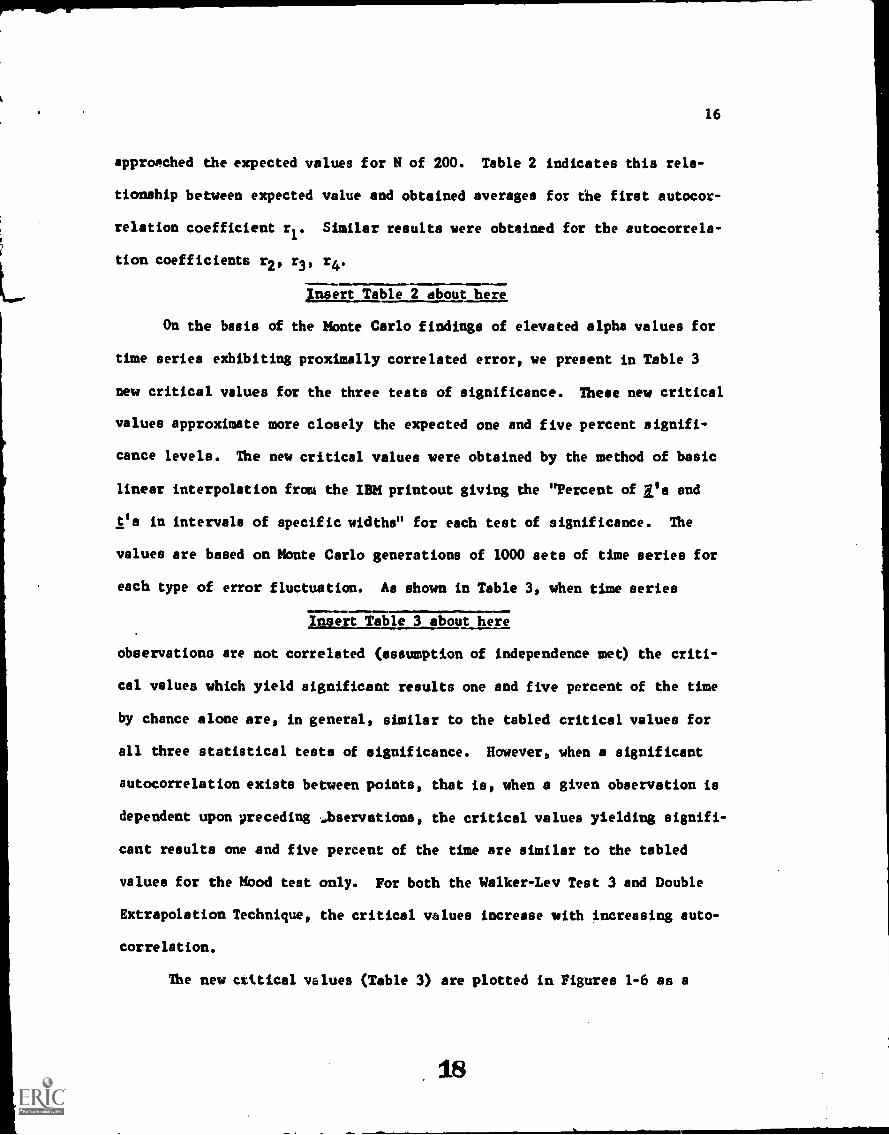
approached the expected values for N of 200. Table 2 indicates this rela-

tionship between expected value and obtained averages for the first autocor-

relation coefficient r1.

Similar results were obtained for the autocorrela-

tion coefficients r2, r3, r4.


On the basis of the Monte Carlo findings of elevated alpha values for

time series exhibiting proximally correlated error, we present in Table 3

new critical values for the three tests of significance. These new critical

values approximate more closely the expected one and five percent signifi-

cance levels. The new critical values were obtained by the method of basic

linear interpolation from the IBM printout giving the "Percent of W's and

is in intervals of specific widths" for each test of significance. The

values are based on Monte Carlo generations of 1000 sets of time series for

each type of error fluctuation. As shown in Table 3, when time series


observations are not correlated (assumption of independence met) the criti-

cal values which yield significant results one and five percent of the time

by chance alone are, in general, similar to the tabled critical values for

all three statistical tests of significance. However, when a significant

autocorrelation exists between points, that is, when a given observation is

dependent upon ,receding ..bservations, the critical values yielding signifi-

cant results one and five percent of the time are similar to the tabled

values for the Mood test only. For both the Walker-Lev Test 3 and Double

Extrapolation Technique, the critical values increase with increasing auto-

correlation.

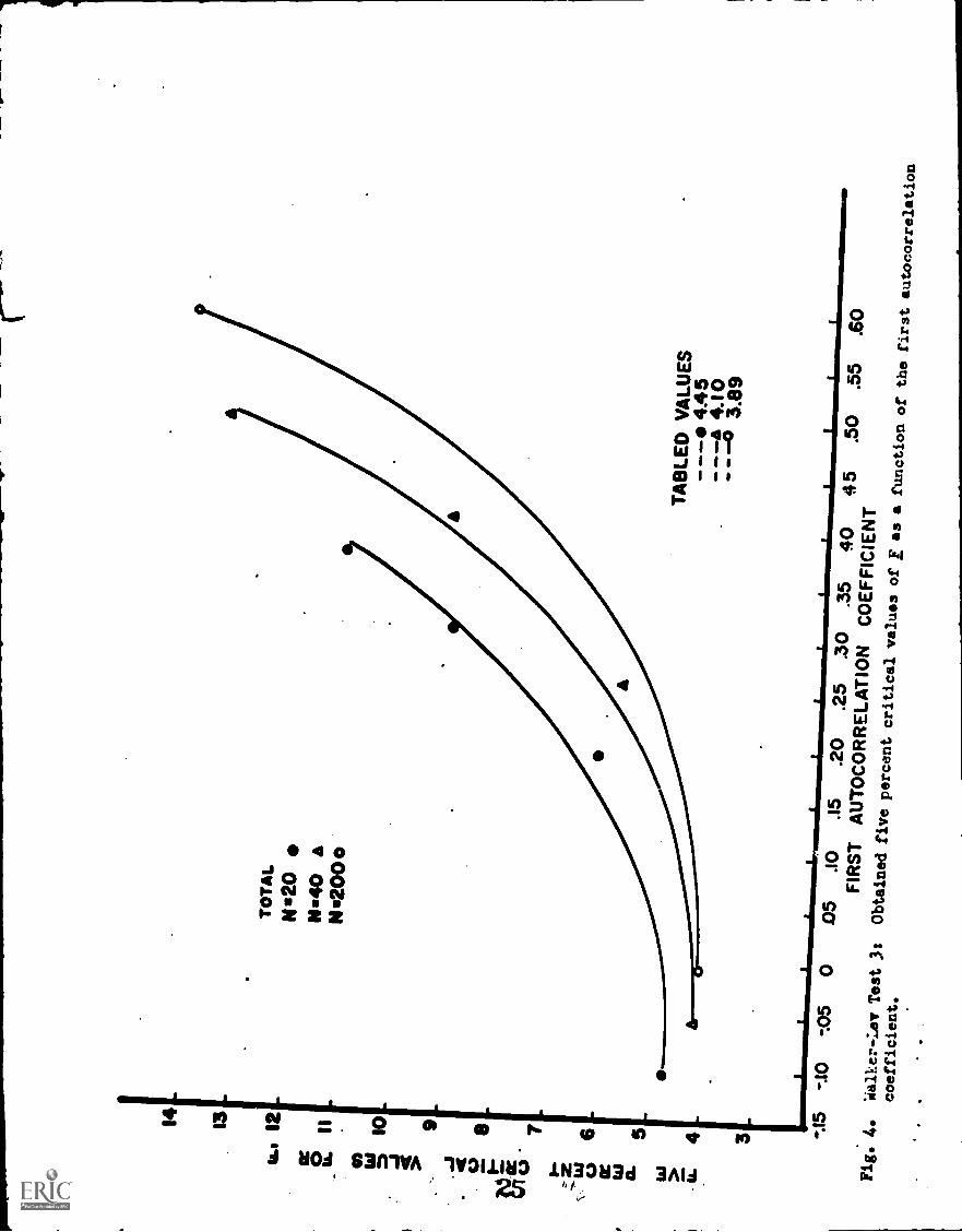
The new cxttical values (Table 3) are plotted in Figures 1-6 as a

is

Table 2

Means and Standard Deviations of the First

Autocorrelation Coefficient r1

Obtained VaJuea Expected Values

Error Type N is 20 N m 40 N 200

Independent x -.11 -.05 -.01 .00SD .21 .16 .07 .03

CorrelatedLag 1 x .18 .26 ..... .33

SD .20 .13 .... .03

CorrelatedLag 2 .x .31 .41 -- .50

SD .22 .14 .... .02

CorrelatedLag 3 x .37 .49 .58 .60

SD .24 .14

1

.06 .02

19

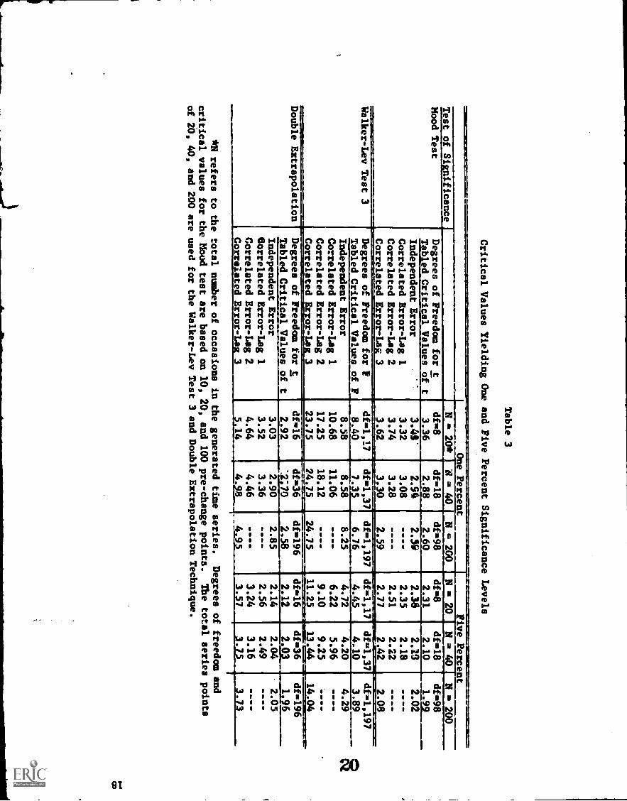
Table 3

Critical Values Yielding One and Five Percent Significance Levels

One Percent

Five Percent

Test of Significance

N = 2017' A = 40

N = 200

N = 20

N .7-45-' N = 200

Mood Test

Degrees of Freedom for t

df=8

df=18

df=98

df=8

df=18

df=98

Tabled Critical Values of t

3.36

2.88

2.60

2.31

2.10

1.99

Independent Error

3.49

2.54

2.39

2.38

2.19

2.02

Correlated Error-Lag 1

3.32

3.08

2.35

2.18

- - --


3.74

3.28

----

2.51

2.22

- - --

Correlated Error-Leg 3

3.62

3.30

2.59

2.77

2.42

2.08

Walker-Lev Test 3

Degrees of Freedom for I

ip==df=1,17

df=1,37

df=1,197

df=1,17

df=1,37

df=1,197

Tabled Critical Values of F

8.40

7.35

6.76

4.45

4.10

3.89

Independent Error

8.58

18.58

8.25

4.72

4.20

4.29

Correlated Error -Lag 1

10.68

11.06

----

6.22

5.96

- - --


17.25

18.12

----

9.10

9.25

1=0,M

ID

Correlated Error-La

323.75

74.75

24.75

11.25

13.44

14.04

Double Extrapolation

Degrees of Freedom for t

df=16

df=36

df=196

df=16

."711-=36

df=196 -...

Tabled Critical Values of t

2.92

.2:70

2.58

2.12

_242_

1.96

Independent Error

3.03

2.90

2.85

2.14

2.04

2.05


3.52

3.36

2.56

2.49


4.64

4.46

- - --

3.24

3.16

.....

Corrdiated Error-Lax 3

5.14

4. 8

4,153a57,3.75

321._

*N refers to the total number of occasions in the generated time series.

Degrees of freedom and

critical values for the Mood test are based on 10, 20, and 100 pre-change points.

The total series points

of 20, 40, and 200 are used for the Walker-Lev Test 3 and Double ExtrapolationTechnique.

19

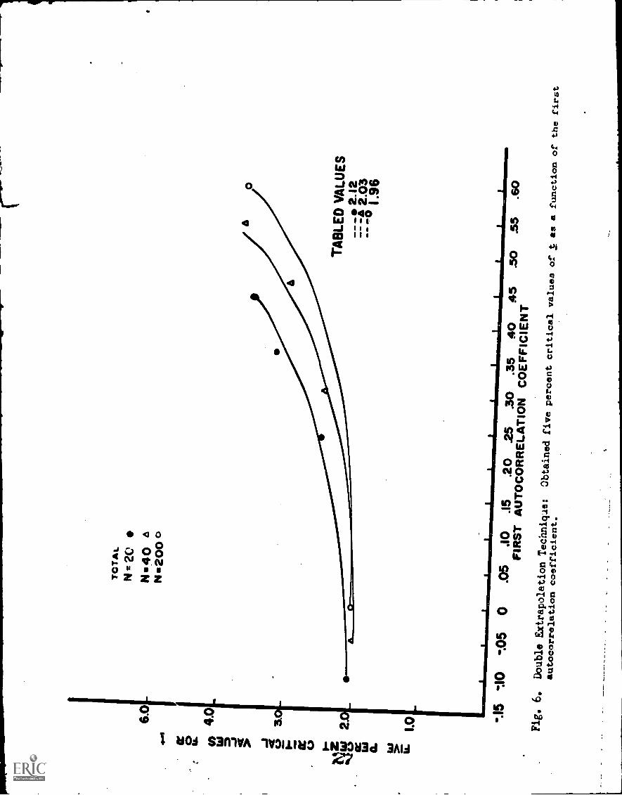
function of the obtained autocorrelation coefficient. As discussed above,

the obtained average r1 is less than the expected value due to greater error

in regression estimates with small N. Figures 1-6 may be used to obtain

approximate one percent and five percent critical values when correlated

error exists between points. The new critical values are found by interpo-

lating on the abscissa using the obtained first autocorrelation coefficient

and on the face of the graph using N. For the Mood test N refers to the

number of pre-change points; for the Walker-Lev Test 3 and Double Extrapola-

tion Technique N refers to the total number of occasions in the time series.

The new critical value is read from the ordinate.

Insert here

Some Utilizations

The tests of significance which we are offering are being applied in

situations in which the visual impression is the usual basis of interpreta-

tion. In some sense, the tests are designed to imitate such judgments, mak-

ing more precise and rationalizing the criteria involved. Thus, the more

variable tha pre-change points, the larger the cross-treatment change must

be to "appear" significant. And holding this constant at a small wriabil-

ity, the longer the :sampling of pre- and post-change observations, the more

confident we are that a given trans-treatment shift is truly exceptional, is

more than a coincidence. These ingredients feature prominently in the tests

we have examined.

In the present study, we have examined only linear hypotheses. Many

times a significant effect in terms of linear hypotheses will appear upon

graphic inspection to be a homogenous curvilinear process with no discontinuity

21

6.0

5.0..0U

.

ta4.0

4It

-J

.t3.0

Er-

i-z2.0

taa.Laz0

1.0

1

PR

E-C

HA

NG

E

Ns 10

N=

20 aN

mo

0

TA

BLE

D V

ALU

ES

-3.36R

I

0

11

11

11

_11

Ii

I

411110 al=

et 2.88- --o 2.60

-.15-JO

-.050

.05.10

.15.20

25.30

.35.40

45.50

.55.60

FIR

ST

AU

TO

CO

RR

ELA

TIO

NC

OE

FF

ICIE

NT

-Fig. 1.

Mbod tests

Obtained one percent criticalvalues of t as a function of the first

autocorrelation coefficient.

6.0

5.0ac

C)

N.

(o)bi3 4.041(

F.: 3.0

ac

z:2 2.0a.I'.

1.0

PRE-CHANG E

Na 10

Ns 20

A

Na 100 0

a0

TA

BLE

D V

ALU

ES

:-

0

-.15-.10

-.050

.05.10

.15.20

.25.30

35.40

45.50

.55.60

FIR

ST

AU

TO

CO

RR

ELA

TIO

N C

OE

FF

ICIE

NT

Fig. 2.

1bod tests Obtained five percent critical values of t as a function of the first autocorrelation coefficient.

26.

24.

IAA

22 20.

18

ot16

F-

4.)

14 12-

tt a.10

_

8 6.

TO

TA

LN

*20

N.4

0N

*200

0

TA

BLE

D V

ALU

ES

....A

I 8.4

07.

356.

76

-.15

-.10

-.05

0

Fig. 3.

.05

.10

.15

.20

.25

.30

.35

.40

.45

.50

.55

.60

FIR

ST

AU

TO

CO

RR

ELA

TIO

NC

OE

FF

ICIE

NT

WalkerLev Test 3:

Obtained one

percent critical values of Fas a function of the first

autocorrelation

coefficient.

14 13

ILI 1

2

10 9

3

TO

TA

LN

20

N.4

0N

u20

0

TA

BLE

D V

ALU

ES

-4.

45--

64.

104"

3.8

9

-.15

-.10

-.05

05.1

0.1

5.2

0.2

5.3

0.3

540

45.5

0.5

5.6

0F

IRS

TA

UT

OC

OR

RE

LAT

ION

CO

EF

FIC

IEN

TFig. 4.

'sialker-Lev Test 3:

Obtained fivepercent criticalvalues of Fas a function of

the firstautocorreletion

coefficient.

6.0

5.0

C)66 Id" 0 4

-J 4 °

3.0

CI wej

2.0

W a. O1.

0

TO

TA

LN

a20

Pi 4

0 es

Na2

00o

TA

BLE

D V

ALU

ES

2.92

---

a 2.

70--

-o 2

.58

.15

JO.0

50

.05

.10

.15

.20

25.3

0.3

540

45.5

0.5

5.6

0F

IRS

T A

UT

OC

OR

RE

LAT

ION

CO

EF

FIC

IEN

TFig. 5.


Technique:

Obtained one

percent critical values of t

as a function of the first


6.0

*el

gt (0)

4.0

W Ea 0 3. 2

ac ta a.

TO

TA

LN

2C

N40

aN

=20

00

TA

BLE

D V

ALU

ES

___

2.12

-* 2

.03

1.96

-.15

10

-.05

0.0

5.1

0.1

5.2

0.2

5.3

0.3

540

45.5

0.5

5.6

0F

IRS

T A

UT

OC

OR

RE

LAT

ION

CO

EF

FIC

IEN

TFig. 6.


Technique:

Obtained fivepercent critical valuesof t as a function of

the first


26

at the treatment point. Usually one will not have sufficient degrees of

freedom to test curvilinear hypotheses. For these and other reasons, it

seems best to accompany tests of significance with graphic presentations.

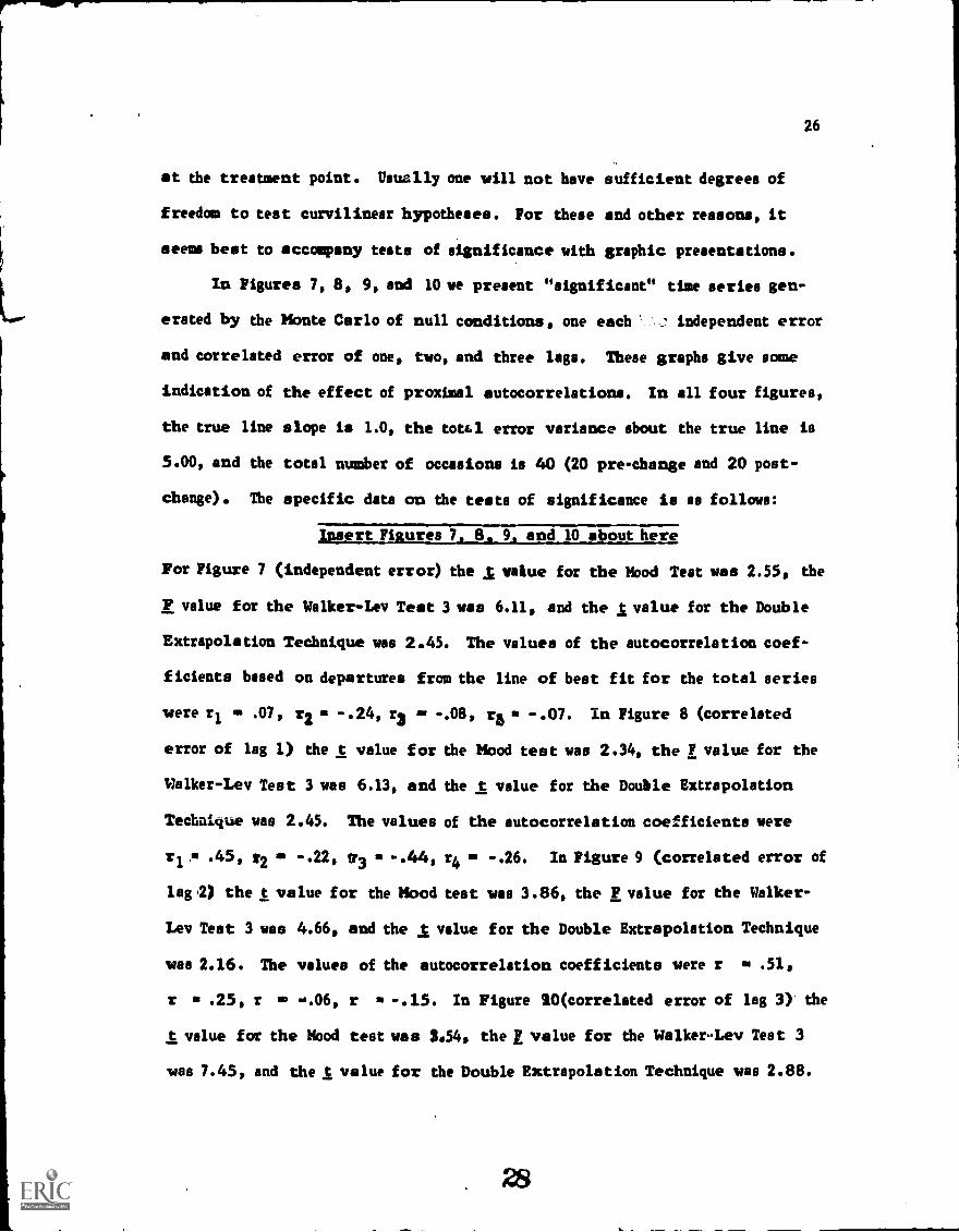
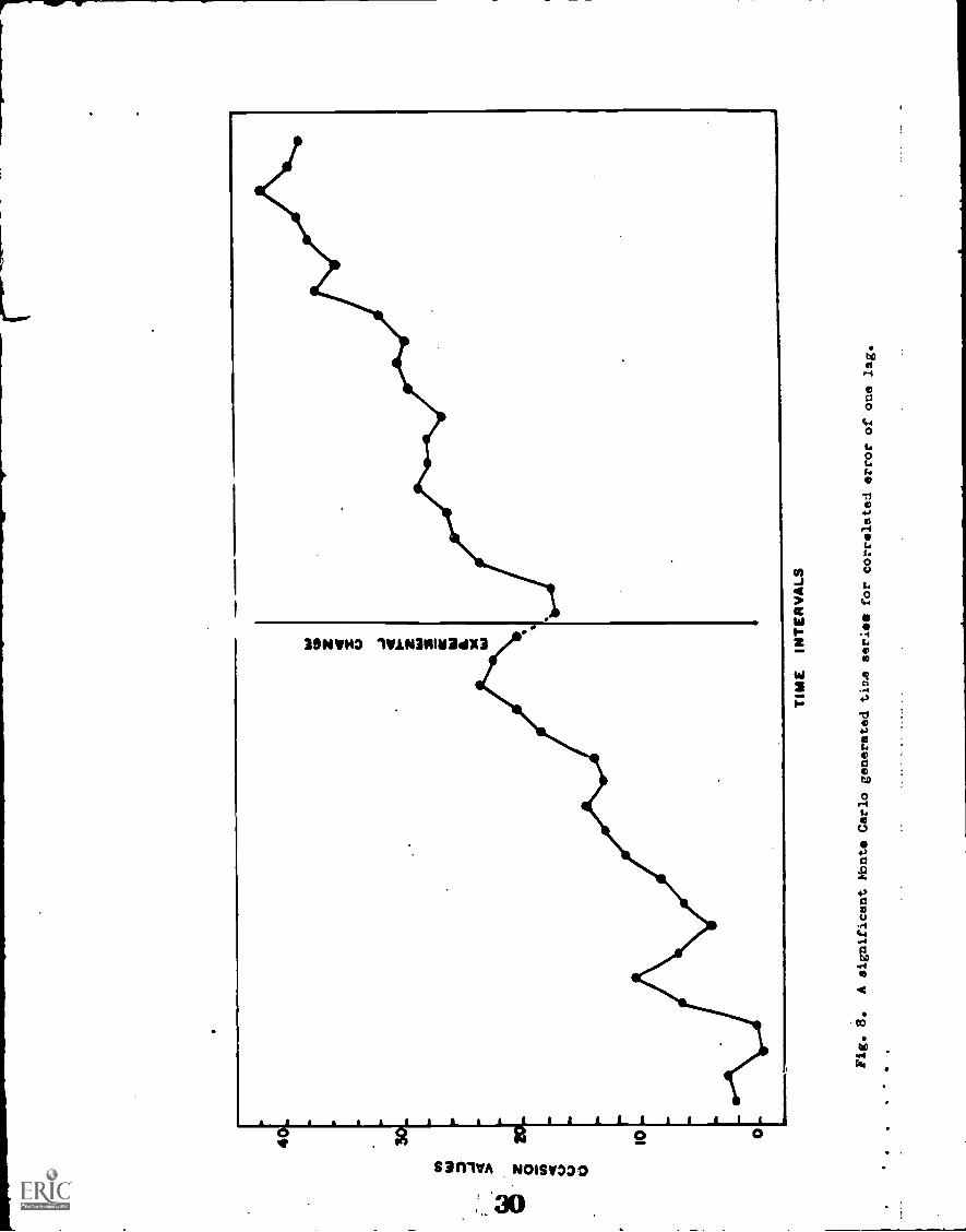
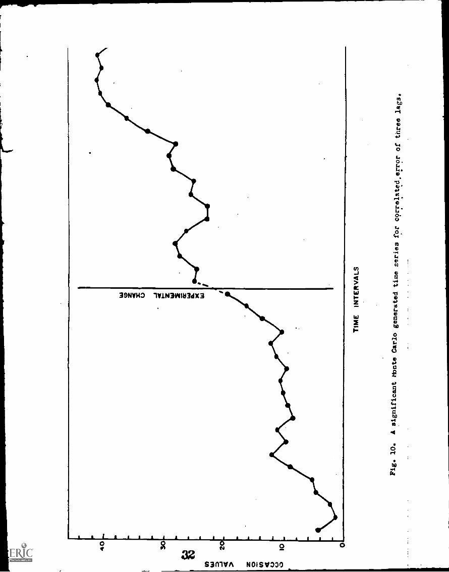
In Figures 7, 8, 9, and 10 we present "significant" time series gen-

erated by the Monte Carlo of null conditions, one each independent error

and correlated error of one, two, and three lags. These graphs give some

indication of the effect of proximal autocorrelationa. In all four figures,

the true line slope is 1.0, the total error variance about the true line is

5.00, and the total number of occasions is 40 (20 pre-change and 20 post-

change). The specific data on the teats of significance is as follows:

Insert Fi urea 7 8 9 and 10 about here

For Figure 7 (independent error) the Imbue for the Mood Teat wee 2.55, the

F value for the Walker-Lev Test 3 was 6.11, and the t value for the Double

Extrapolation Technique was 2.45. The values of the autocorrelation coef-

ficients based on departures from the line of best fit for the total series

were r1 as .07, r2 -.24, r3 -.08, re, -.07. In Figure 8 (correlated

error of lag 1) the t value for the Mood teat was 2.34, the F value for the

Walker-Lev Teat 3 was 6.13, and the t value for the Double Extrapolation

Technique was 2.45. The values of the autocorrelation coefficients were

r1 .45, x2 a. -.22, 73 -.44, r4 al -.26. In Figure 9 (correlated error of

lag .2) the t value for the Mood test was 3.86, the F value for the Walker-

Lev Test 3 was 4.66, and the I value for the Double Extrapolation Technique

was 2.16. The values of the autocorrelation coefficients were r .51,

r .25, r x.06, r -.15. In Figure 20(correlated error of lag 3) the

t value for the Mood teat was 3.54, the F value for the Walker-Lev Test 3

was 7.45, and the t value for the Double Extrapolation Technique was 2.88.

10

TIN

E IN

TE

RV

ALS

Mg. 7. A significant !bate Carlogenerated time series for independenterror.

2

TIM

E IN

TE

RV

ALS

Fig. 8.

A significant Niante Carlo generated time series forcorrelated error of one lag.

40

.

2 O.

I

TIME INTERVALS

Pig. 9.

A significant Monte Carlo generated time series for correlated error of two lags.

40 30

2 I0 0

I

TIME INTERVALS

Fig, 10.

A significant Mbnte Carlo

generated time series for correlated

error of three lags.

..

.

31

The values of the autocorrelation coefficients were r1 .76, r2 gm .50,

r3 .20, r4 v.14.

To further illustrate utilizations of these tests of significance,

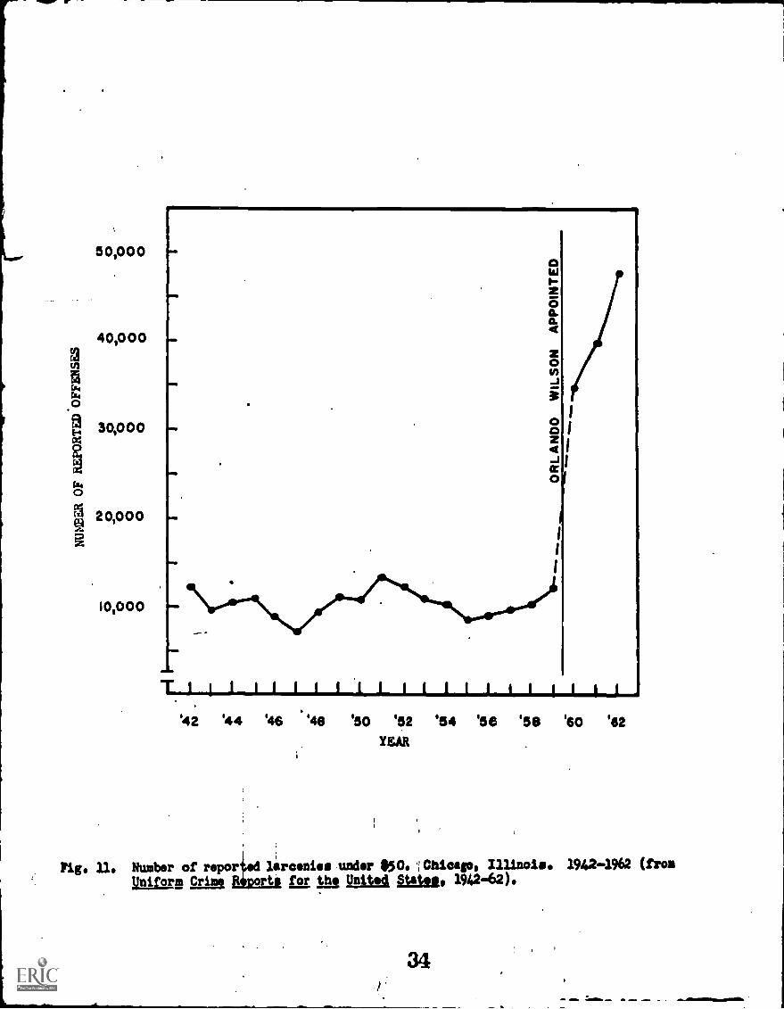
in Figure 11, 12, 13, and 14 we present actual data. In general, these

figures represent instances in which the tests of significance confirm judg-

ments of effect which had been made on the basis of visual inspection alone.

Insert Fissures 11 1213. and 14 about here

Figures 11 and 12 represent Chicago crime rate statistics for the

categories of "Larceny under $50" and "Murder and non-negligent manslaughter,"

respectively (from Uniform Crime Reports for the U.S., 1942-1962). On Febru-

ary 22, 1960, it was announced that Orlando Wilson had been selected as

Superintendent of the Chicago Police Force (New York Times, February 23,

1960, page 1). He became acting commissioner on March 2, 1960. It was sub-

sequently reported that "Recorded crime in Chicago increased 83.7% in the

first 10 months of 1960, police statistics indicated today. The officials

refused to say how much of the increase was due to a higher crime rate and

how much to improved record keeping by police" (New York Times, December 17,

1960, page 34). In Figure 11, all statistical tests indicate that the

observed increase in recorded "Larceny under $50" was significant. The t

value for the Mood teat was 12.54, the F value for the Walker-Lev Test 1 was

51.59, the F value for the Walker-Lev Test 3 was 157.76, and the t value for

the Double Extrapolation Technique was 9.12. The value of the first auto-

correlation coefficient based on departures from separate pre- and post-

change regression lines was .43. However, in Figure 12 where the effect

seems to start several observations before Orlando Wilson's appointment,

none of the statistical tests' were significant. The t value for the Mood

33

50,000

40,000

O

30,000oC

fl 20,000

10,000

'42 '44 '46 '46 '50 '52 '54 '56 '58 '60 '62

YEAR

Fig. 11. Number of repotied larcenies under $50. .:Chloago, Illinois. 1942-1962 (fromUniform Crime ft ports for the Unite4 States, 1942 -62).

400

350

tal

C.44 300

250

200

150

z0- J

0Oz4- JCZ0

'42 '44 '46 '48 '50 '52 '54 '56 '59 '60 '82YEAR

Fig. 12. Number of reported murders and nonnegligent mouselaUghters.. Chicago, Illinois.1942-1962 (from Uniform caw Report/ ar kg Unites* states, 1942-62).

2

U.0

560

550

540

530

520

510

Ti'50 .52 '54 '56

YEAR

'S

Fig. 13. Number of hospitalised mental patients in the United States before and afterthe advent of tranquilizing drugs (from Britannia& Book at gs ha, 3.2f1).

s--

.10

.60

.70

.60

.50

40

.30

.20

-.10

s

164I

a 3 4 5

MINIS@ SESSIONS

Fig. 14. Reliability 'coefficients for the struotiure dissension of the Leadership OpinionQuestionnaire for training sessions before and after the assassination ofPresident Kennedy (from Ayers; 1964).

test was 1.10, the F valuea,fbr the Walker-Lev tests 1 and 3 were .03 and

2.69, respectively, and the t value for the Double Extrapolation Technique

was .82. The value of the first autocorrelation coefficient based on

departures from the total series regression line was .15.

Figure 11 represents the number of hospitalized mental patients in the

United States before and after the advent of the use of tranquilizing drugs

(from Britannic. Book of the Year, 1965). The significant statistical tests

were the Walker-Lev Test 2 (F gm 213.75) and the Mood test (t 7.40). The F

value for the Walker-Lev test 3 was .26 and the t value for the Double Extra-

polation technique was 1.38. The value of the first autocorrelation coeffi-

cient based on differences from the separate pre- and post-change regression

lines was .52.

Figure 14 represents reliability coefficients for the Structure Dimen-

sion of a Leadership Opinion Questionnaire which was administered at the

beginning and end of each of eight week-long training sessions. The train-

ing session groups ranged in size from 22 to 55 participants. Classes for

the week-long sessions were given in the Spring and Autumn months of 19163

and are indicated in chronological order on the abscissa of the graph. For

the eighth training session, pretesting took place on Noveraber 18, 1963,

whereas posttesting occurred on Friday afternoon, November 22, at the close

of the session. During the lunch period, 1:30-2:30 P.M., the participants

had watched and listened to the memorable events being reported from Dallas,

Texas (from Ayers, 1966). Since only one post-change point is given, only

the Mood teat of significance is applicable. The obtained t value for the MAL.

teat was 6.24 with 5 df, thus, confirming the impression of effect. The

value of the first autocorrelation coefficient based on differences from the

38

37

separate pre- and post-change regression lines was .12.

As the above examples of actual time series illustrate, the tests of

significance are not equally applicable to all time series data. The several

possible time series of Figure 15 indicate this. The time series of Al and

Insert 11146.1e151il t heree

A2 are instances of sustained post-change effect involving a change in inter-

cept; whereas, 111 and B2 show an initial jump and subsequent return to pre-

change conditions. If theoretical expectations are appropriate to using a

series of points in the post-change period (as they would be in Al and A2)

the Walker-Lev Test 3 and Double Extrapolation Technique would be most suit-

able. These two tests would not be used in instances of theoretical, expects.

tiona similar to Ill and B2 where only the Mood Test of the significance of

the first-post change observation from a trend extrapolated from the pre-

change observations would be appropriate.

A times series analysis seems most suitable in instances discussed

above. In Cl, C2, and C3 where the post-treatment effect involves a change

in slope and, generally, of intercept, the possibility of a curvilinear rela-

tionship or cyclical trend is more difficult to rule out. A large number of

pre- and post-treatment observations would be helpful in eliminating these

possibilities. All three statistical testa and, in particular, the Walker-

Lev Test 1, may be used, but they may yield conflicting results. For example,

the double extrapolation technique can be used to indicate if the pre- and

post-regression lines coincide at time to midway between the last pre-change

and first post-change point. However, extension of the regression lines of

C2 will show that the two lines coincide at time to, although pre- and post-

regression lines are dissimilar.

ik.4041"1""I\

At

A2

el

82

1410"'"'".°

se/C3

CI

tm:3 in;-2 tre;1 an trilui In;2 tn;3 tnti.40

DI

EXPERIMENTAL CHANGE

Fig. 15. Soros possible outcome patterns for the interrupted time aeriesexperiment.

I4)

39

Similarly, the first post-change point may not differ greatly from

that predicted by the pre-change values, yet a continuing and substantial

increase or decrease in subsequent post-change values may suggest an effect.

In instances of delayed effect, such as Dl, ambiguity is introduced

into the interpretation of significance (as the time interval between the

treatment and its effect increases the plausibility of rival hypotheses also

increases). However, if the experimenter specifies in advance the exact

relationship between the introduction of the treatment and the manifestation

of its effect, the pattern indicated by time-series Dl could be almost as

definitive as that in which immediate effect is expected.

41

40

References

Ayers, Arthur (Westinghouse Electric Corporation). Letter in American

atchol., 19, 1964, p. 353.

Britannica Book of the Year, 1965. Chicago, Encyclopedia Brittanica, 1965,

p. 626.

Campbell, D. T. From description to experimentation. In C. W. Harris (Ed.),

Problems in measuring change, Madison, Wis.: University of Wisconsin

Press, 1963, pp. 212-242.

Campbell, D. T., and Stanley, J. S. Experimental and quasi-experimental

designs for research on teaching. In N. L. Gage (Ed.), Handbook of

research on teaching. Chicago: Rand McNally, 1963, pp. 171-246.

Holtzman, W. H. Statistical models for the study of change in the single

case. In C. W. Harris (Ed.), Problems in measuring change, Madison,

Wis.: University of Wisconsin Press, 1963, pp. 199-211.

Mod, A. F. Introduction to the theory of statistics. New York: McGraw-

Hill, 1950.

Sween, Joyce A., and Campbell, D. T. The interrupted time series as quasi-

experiment: three tests of significance. Northwestern 1niversity,1965.

Uniform Crime Reports for the United States. Issued by the Federal Bureau

of Investigation, United States Dept. of Justice, Washington, D.C.

Walker, Helen IC, and Lev, J. Statistical inference. New York: molt, 1953.

42

41

Footnotes

lA preliminary Investigation of the Clayton Test using 100 sets of gen-

erated time series (total fi 40, true line-slope - 1.00, total error vari-

ance - 5.00) yielded alpha values greater than the expected one and five per-

cents when no dependency between points was built in (independent error).

The percents of significant instances exceeding the five percent tabled crit-

ical value of F were 17%, 36%, 5314 and 61% for independent error, lag 1,

lag 2, and lag 3 correlated errors, respectively. In lieu of this prelimin-

ary finding, the Clayton test was not considered a useful significance test

in the interrupted time series situation and it was eliminated from further

Monte Carlo investigation.

In a similar preliminary investigation, the Walker-Lev Test 1 yielded

4% (independent error), 16% (lag 1 error), 26% (lag 2 error), and 34% (lag 3

error) false-positive instances above the five percent tabled critical value

of F. Although the Walker-Lev Teat 1 yielded results similar to those

obtained in a preliminary investigation of the Walker-Lev Test 3, it was

eliminated in the final 1000 set investigation. Preference was given to the

Walker-Lev Test 3 because of the more restricted usefulness of Test 1. Since

the Walker-Lev Test 1 is a test of slope differences only it is more diffi-

cult to rule out rival curvilinear hypothesis in cases of significance.

The Walker-Lev Test 2 was not used because a test of the null hypothe-

sis of zero slope is not of general interest as a test of significance in

the time series situation.

Documents

investigate the appropriateness of several tests of