Embed Size (px)
Citation preview

INVERTED INDEX CONSTRUCTION
Dr. Gjergji Kasneci | Introduction to Information Retrieval | WS 2012-13 1

Outline
Intro
Basics of probability and information theory
Retrieval models
Retrieval evaluation
Link analysis
From queries to top-k results Query processing
Index construction
Top-k search
Social search
Dr. Gjergji Kasneci | Introduction to Information Retrieval | WS 2012-13 2
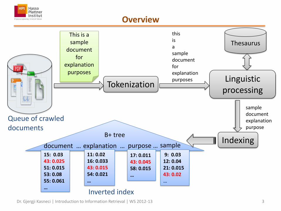
Overview
Dr. Gjergji Kasneci | Introduction to Information Retrieval | WS 2012-13 3
Tokenization Linguistic
processing
Indexing
Inverted index
This is a sample
document for
explanation purposes
this is a sample document for explanation purposes
sample document explanation purpose
B+ tree
document … 15: 0.03 43: 0.025 51: 0.015 53: 0.08 55: 0.061 …
explanation … 11: 0.02 16: 0.033 43: 0.015 54: 0.021 …
purpose … sample
17: 0.011 43: 0.045 58: 0.015 …
9: 0.03 12: 0.04 21: 0.015 43: 0.02 …
Thesaurus
Queue of crawled documents
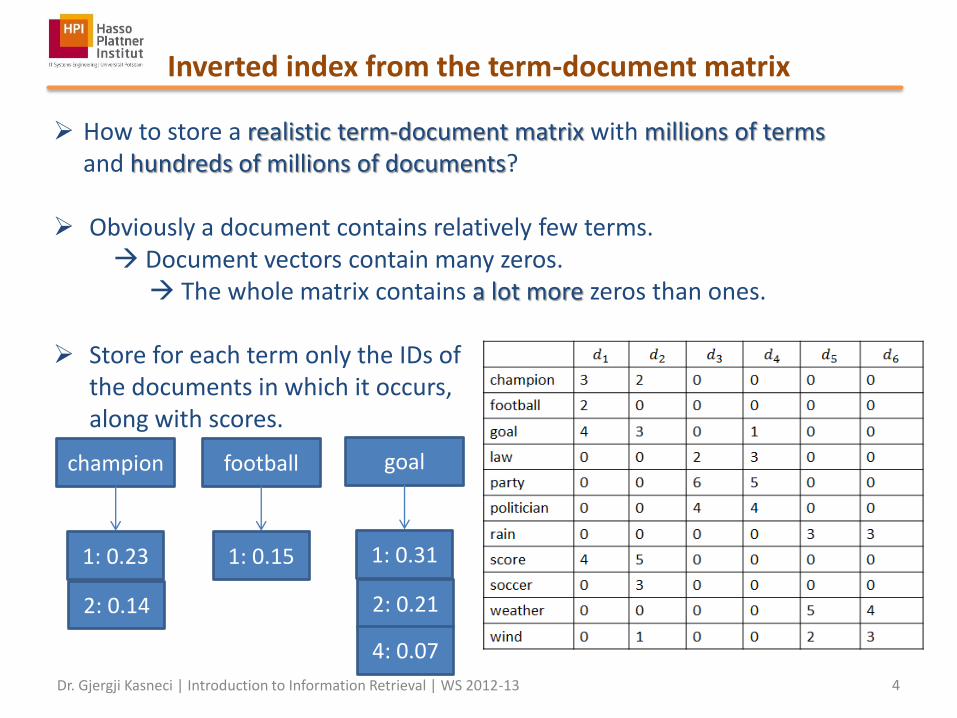
Inverted index from the term-document matrix
Dr. Gjergji Kasneci | Introduction to Information Retrieval | WS 2012-13 4
How to store a realistic term-document matrix with millions of terms and hundreds of millions of documents? Obviously a document contains relatively few terms. Document vectors contain many zeros. The whole matrix contains a lot more zeros than ones. Store for each term only the IDs of the documents in which it occurs, along with scores.
champion
1: 0.23
2: 0.14
football
1: 0.15
goal
1: 0.31
2: 0.21
4: 0.07

Important steps for index constructions
Sort documents by terms.
Merge multiple term occurrences in a single document but maintain position information and add frequency information.
Construct corpus vocabulary with entries of the form 𝑡𝑒𝑟𝑚, #𝑑𝑜𝑐𝑠, 𝑐𝑜𝑟𝑝𝑢𝑠_𝑐𝑜𝑢𝑛𝑡
Construct for every term postings with entries of the form
𝑑𝑜𝑐𝐼𝐷, 𝑐𝑜𝑢𝑛𝑡, 𝑙𝑖𝑠𝑡[pos1, offsets. . ]
Why are position-based postings better than postings that store biwords or longer phrases (e.g., ‘stanford university’ or ‘hasso plattner institute’)?
All steps involve distributed computations (e.g., through MapReduce methods)
Dr. Gjergji Kasneci | Introduction to Information Retrieval | WS 2012-13 5

Example
Dr. Gjergji Kasneci | Introduction to Information Retrieval | WS 2012-13 6
term #docs #
champion 2 5
football 1 2
goal 3 8
law 2 5
party 2 11
politician 2 8
rain 2 6
score 2 9
soccer 1 3
weather 2 9
wind 3 6
docID freq
1 3
2 2
1 2
1 4
2 3
4 1
3 2
4 3
3 6
4 5
.
.
.
.
.
.
Vocabulary Frequency-based postings (offsets omitted) Pointers
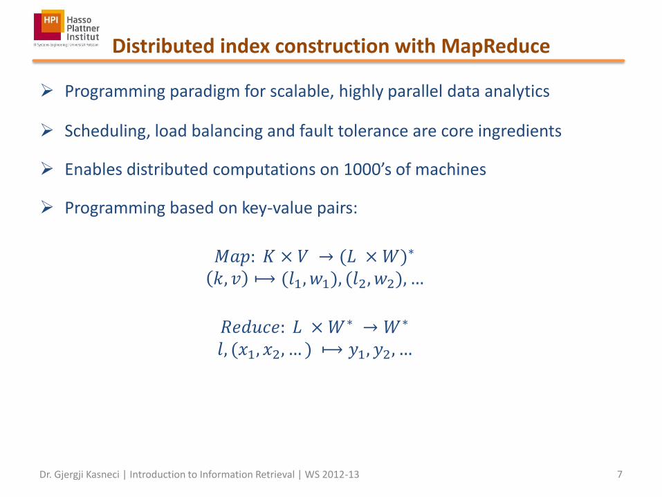
Distributed index construction with MapReduce
Programming paradigm for scalable, highly parallel data analytics
Scheduling, load balancing and fault tolerance are core ingredients
Enables distributed computations on 1000’s of machines
Programming based on key-value pairs:
𝑀𝑎𝑝: 𝐾 × 𝑉 → (𝐿 × 𝑊)∗ 𝑘, 𝑣 ⟼ (𝑙1, 𝑤1), (𝑙2, 𝑤2), …
𝑅𝑒𝑑𝑢𝑐𝑒: 𝐿 × 𝑊∗ → 𝑊∗ 𝑙, (𝑥1, 𝑥2, … ) ⟼ 𝑦1, 𝑦2, …
Dr. Gjergji Kasneci | Introduction to Information Retrieval | WS 2012-13 7

MapReduce implementations: PIG (Yahoo), Hadoop (Apache), DryadLinq (Microsoft),
Facebook Corona
Possible MapReduce Infrastructure for Indexing
Dr. Gjergji Kasneci | Introduction to Information Retrieval | WS 2012-13 8
Source: Introduction to Information Retrieval
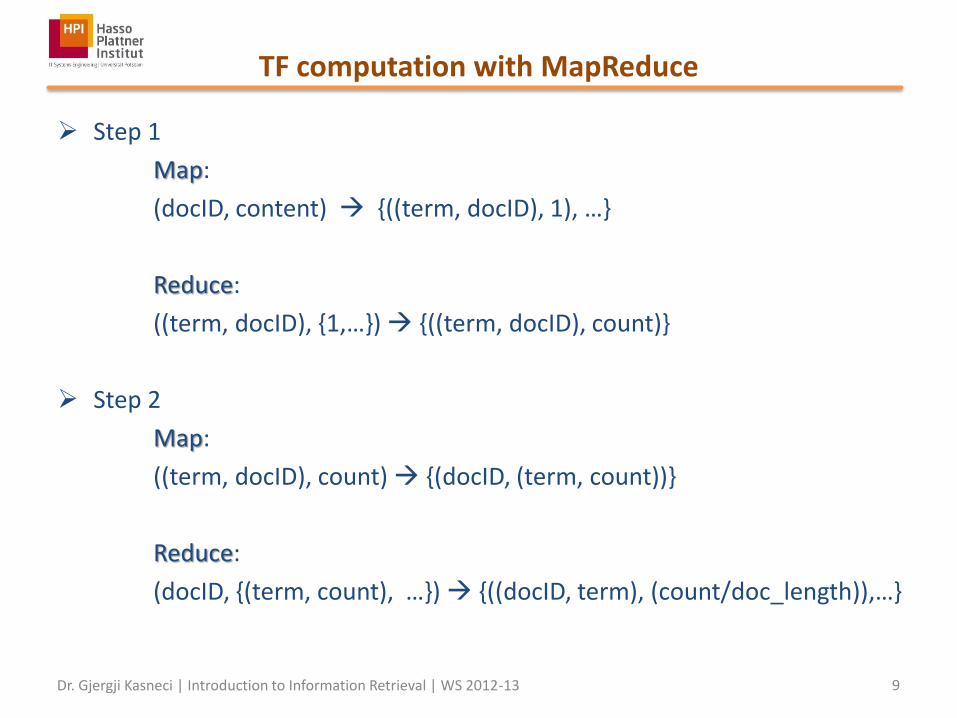
TF computation with MapReduce
Step 1
Map:
(docID, content) {((term, docID), 1), …}
Reduce:
((term, docID), {1,…}) {((term, docID), count)}
Step 2
Map:
((term, docID), count) {(docID, (term, count))}
Reduce:
(docID, {(term, count), …}) {((docID, term), (count/doc_length)),…}
Dr. Gjergji Kasneci | Introduction to Information Retrieval | WS 2012-13 9
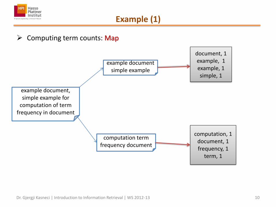
Example (1)
Computing term counts: Map
Dr. Gjergji Kasneci | Introduction to Information Retrieval | WS 2012-13 10
example document, simple example for
computation of term frequency in document
example document simple example
computation term frequency document
document, 1 example, 1 example, 1 simple, 1
computation, 1 document, 1 frequency, 1
term, 1

Example (2)
Computing term counts: Reduce
Dr. Gjergji Kasneci | Introduction to Information Retrieval | WS 2012-13 11
document, 1 example, 1 example, 1 simple, 1
computation, 1 document, 1 frequency, 1
term, 1
example, {1, 1}
simple, {1}
computation, {1}
frequency, {1}
term, {1}
document, {1,1}
example, 2
simple, 1
computation, 1
frequency, 1
term, 1
document, 2
document, 2 example, 2
simple, 1 computation, 1
frequency, 1 term, 1
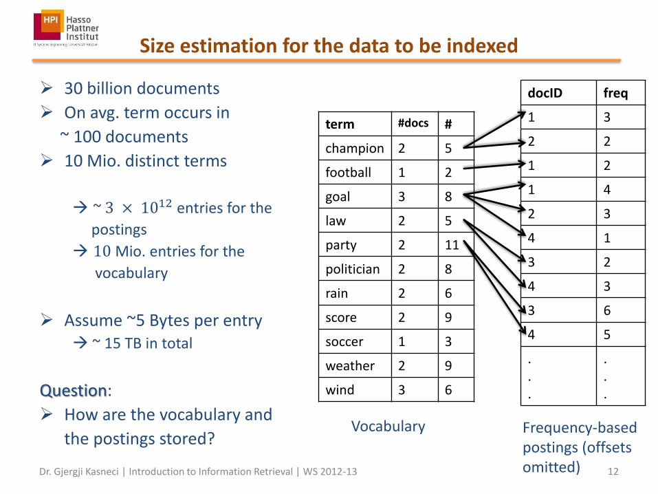
Size estimation for the data to be indexed
30 billion documents
On avg. term occurs in
~ 100 documents
10 Mio. distinct terms
~ 3 × 10¹² entries for the
postings
10 Mio. entries for the
vocabulary
Assume ~5 Bytes per entry ~ 15 TB in total
Question:
How are the vocabulary and
the postings stored?
Dr. Gjergji Kasneci | Introduction to Information Retrieval | WS 2012-13 12
term #docs #
champion 2 5
football 1 2
goal 3 8
law 2 5
party 2 11
politician 2 8
rain 2 6
score 2 9
soccer 1 3
weather 2 9
wind 3 6
docID freq
1 3
2 2
1 2
1 4
2 3
4 1
3 2
4 3
3 6
4 5
.
.
.
.
.
.
Vocabulary Frequency-based postings (offsets omitted)
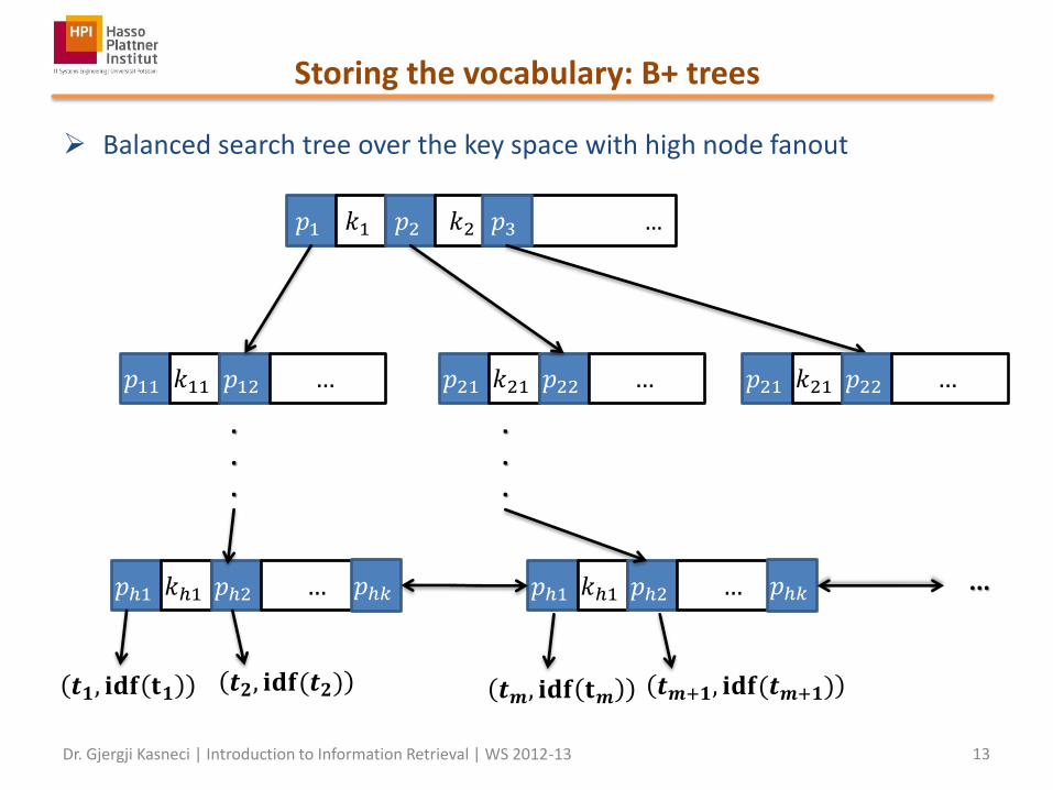
Storing the vocabulary: B+ trees
Balanced search tree over the key space with high node fanout
Dr. Gjergji Kasneci | Introduction to Information Retrieval | WS 2012-13 13
𝑝1 𝑘1 𝑝2 𝑘2 … 𝑝3
𝑝11 𝑘11 𝑝12 … 𝑝21 𝑘21 𝑝22 …
.
.
.
𝑝21 𝑘21 𝑝22 …
𝑝ℎ1 𝑘ℎ1 𝑝ℎ2 … 𝑝ℎ𝑘 𝑝ℎ1 𝑘ℎ1 𝑝ℎ2 … 𝑝ℎ𝑘
.
.
.
...
𝒕𝟏, 𝐢𝐝𝐟 𝐭𝟏 𝒕𝟐, 𝐢𝐝𝐟(𝒕𝟐) 𝒕𝒎, 𝐢𝐝𝐟 𝐭𝒎 𝒕𝒎+𝟏, 𝐢𝐝𝐟(𝒕𝒎+𝟏)
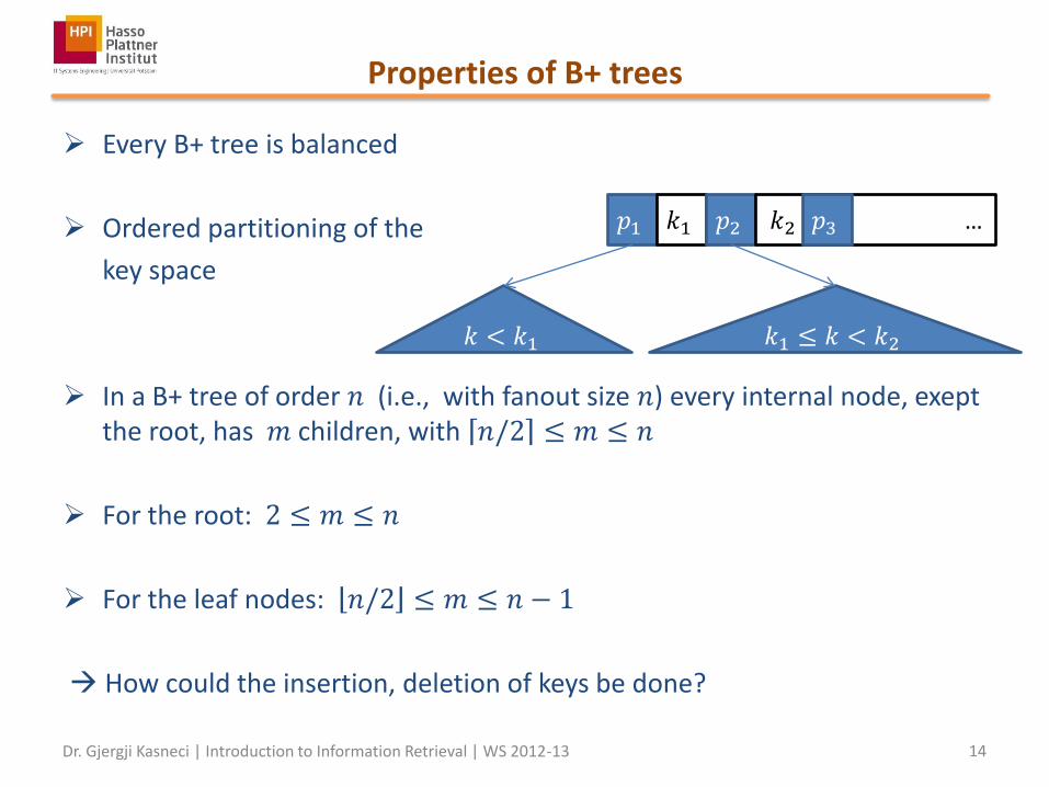
Properties of B+ trees
Every B+ tree is balanced
Ordered partitioning of the
key space
In a B+ tree of order 𝑛 (i.e., with fanout size 𝑛) every internal node, exept the root, has 𝑚 children, with 𝑛/2 ≤ 𝑚 ≤ 𝑛
For the root: 2 ≤ 𝑚 ≤ 𝑛
For the leaf nodes: 𝑛/2 ≤ 𝑚 ≤ 𝑛 − 1
How could the insertion, deletion of keys be done?
Dr. Gjergji Kasneci | Introduction to Information Retrieval | WS 2012-13 14
𝑝1 𝑘1 𝑝2 𝑘2 … 𝑝3
𝑘 < 𝑘1 𝑘1 ≤ 𝑘 < 𝑘2
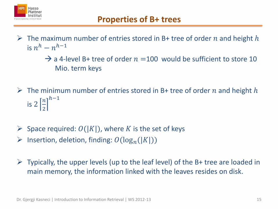
Properties of B+ trees
The maximum number of entries stored in B+ tree of order 𝑛 and height ℎ is 𝑛ℎ − 𝑛ℎ−1
a 4-level B+ tree of order 𝑛 =100 would be sufficient to store 10 Mio. term keys
The minimum number of entries stored in B+ tree of order 𝑛 and height ℎ
is 2𝑛
2
ℎ−1
Space required: 𝑂(|𝐾|), where 𝐾 is the set of keys
Insertion, deletion, finding: 𝑂(log𝑛(|𝐾|))
Typically, the upper levels (up to the leaf level) of the B+ tree are loaded in main memory, the information linked with the leaves resides on disk.
Dr. Gjergji Kasneci | Introduction to Information Retrieval | WS 2012-13 15
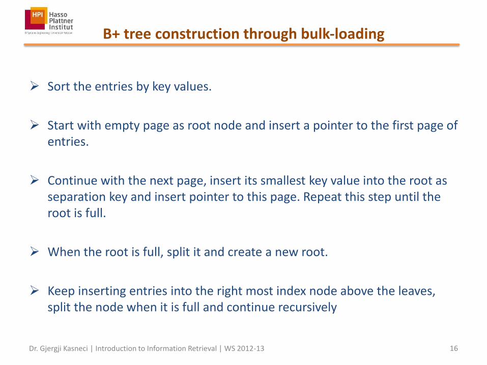
B+ tree construction through bulk-loading
Sort the entries by key values.
Start with empty page as root node and insert a pointer to the first page of entries.
Continue with the next page, insert its smallest key value into the root as separation key and insert pointer to this page. Repeat this step until the root is full.
When the root is full, split it and create a new root.
Keep inserting entries into the right most index node above the leaves, split the node when it is full and continue recursively
Dr. Gjergji Kasneci | Introduction to Information Retrieval | WS 2012-13 16

Index merging
Dr. Gjergji Kasneci | Introduction to Information Retrieval | WS 2012-13 17
Source: Modern Information Retrieval
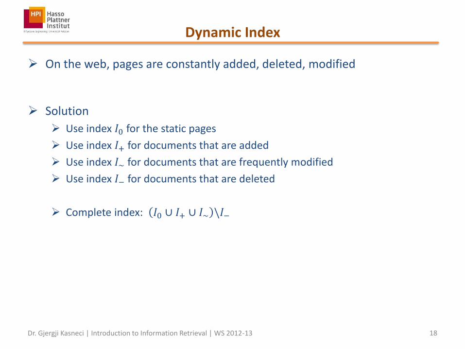
Dynamic Index
On the web, pages are constantly added, deleted, modified
Solution
Use index 𝐼0 for the static pages
Use index 𝐼+ for documents that are added
Use index 𝐼~ for documents that are frequently modified
Use index 𝐼− for documents that are deleted
Complete index: 𝐼0 ∪ 𝐼+ ∪ 𝐼~ \𝐼−
Dr. Gjergji Kasneci | Introduction to Information Retrieval | WS 2012-13 18
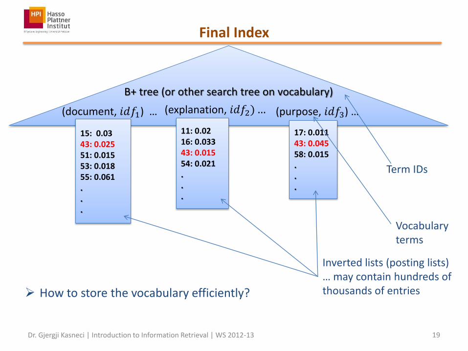
Final Index
Dr. Gjergji Kasneci | Introduction to Information Retrieval | WS 2012-13 19
B+ tree (or other search tree on vocabulary)
(document, 𝑖𝑑𝑓1) …
15: 0.03 43: 0.025 51: 0.015 53: 0.018 55: 0.061 . . .
(explanation, 𝑖𝑑𝑓2) …
11: 0.02 16: 0.033 43: 0.015 54: 0.021 . . .
(purpose, 𝑖𝑑𝑓3) …
17: 0.011 43: 0.045 58: 0.015 . . .
Inverted lists (posting lists) … may contain hundreds of thousands of entries
Term IDs
Vocabulary terms
How to store the vocabulary efficiently?
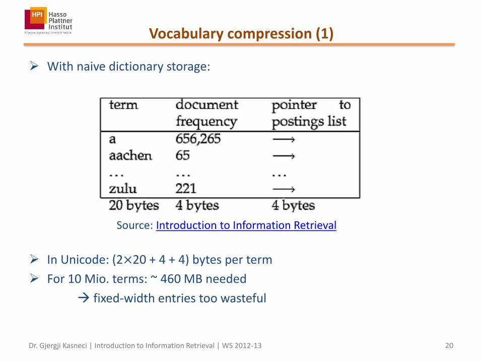
Vocabulary compression (1)
With naive dictionary storage:
In Unicode: (2×20 + 4 + 4) bytes per term
For 10 Mio. terms: ~ 460 MB needed
fixed-width entries too wasteful
Dr. Gjergji Kasneci | Introduction to Information Retrieval | WS 2012-13 20
Source: Introduction to Information Retrieval
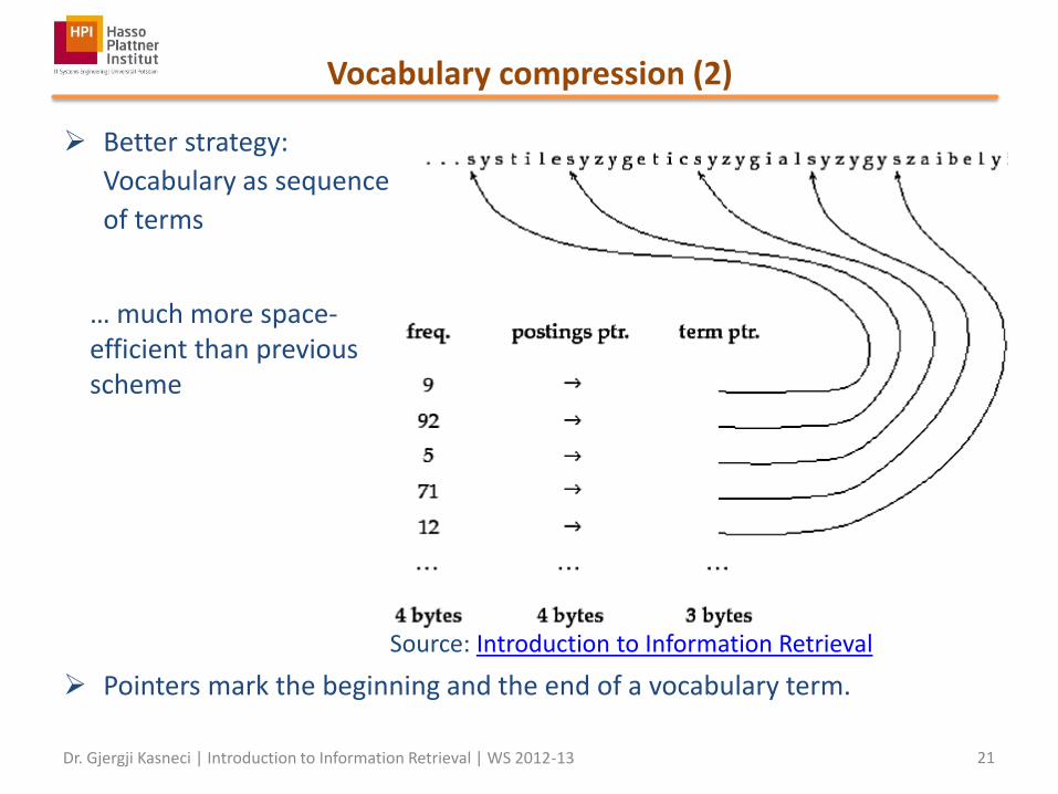
Vocabulary compression (2)
Better strategy:
Vocabulary as sequence
of terms
Pointers mark the beginning and the end of a vocabulary term.
Dr. Gjergji Kasneci | Introduction to Information Retrieval | WS 2012-13 21
… much more space-efficient than previous scheme
Source: Introduction to Information Retrieval
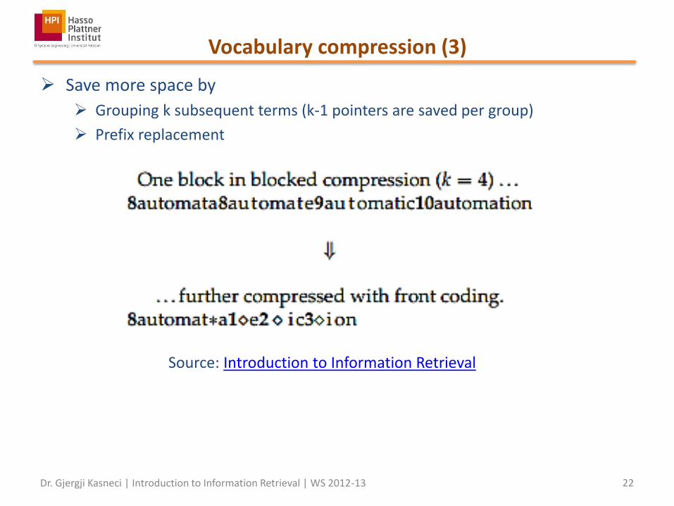
Save more space by
Grouping k subsequent terms (k-1 pointers are saved per group)
Prefix replacement
Vocabulary compression (3)
Dr. Gjergji Kasneci | Introduction to Information Retrieval | WS 2012-13 22
Source: Introduction to Information Retrieval
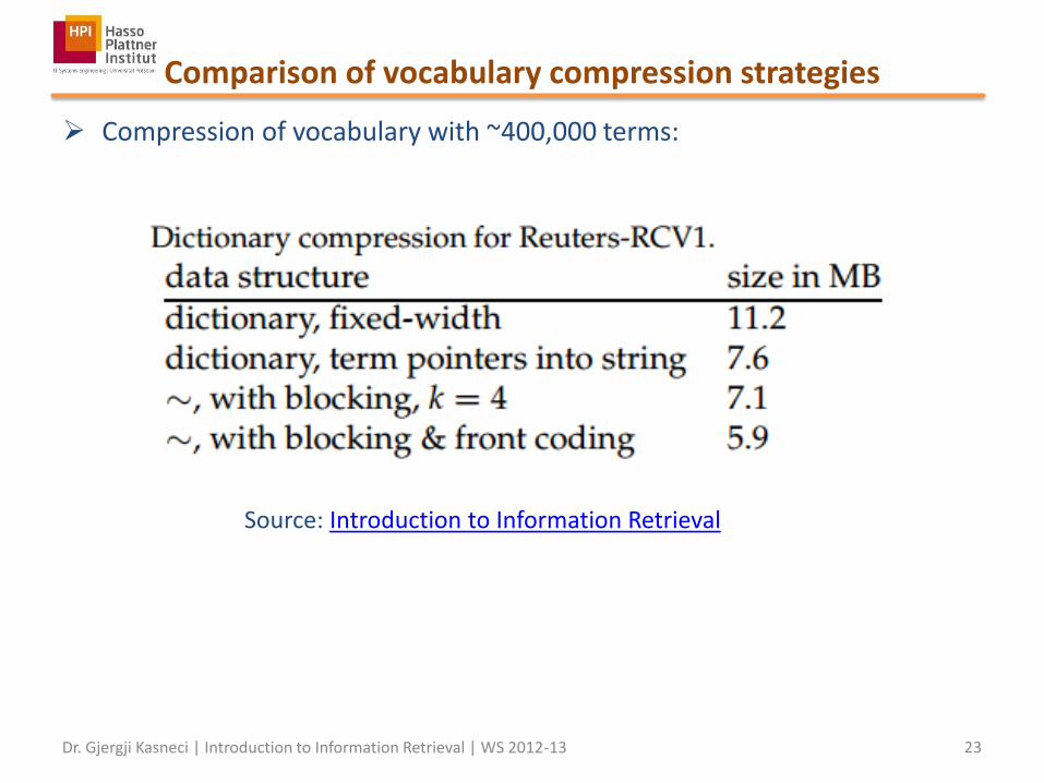
Comparison of vocabulary compression strategies
Dr. Gjergji Kasneci | Introduction to Information Retrieval | WS 2012-13 23
Source: Introduction to Information Retrieval
Compression of vocabulary with ~400,000 terms:

Vocabulary compression with prefix trees
For vocabularies of moderate size (e.g., for in-memory processable size) use tries (conceptually the same as the previous scheme)
Dr. Gjergji Kasneci | Introduction to Information Retrieval | WS 2012-13 24
This is a text. This text has many letters. Terms are made of letters.
d1 d2 d3
letters: (d2, 1, [5]), (d3, 1, [5])
m a d
n
made: (d3, 1, [3])
many: (d2, 1, [4]) t
e text: (d1, 1, [4]), (d2, 1, [2])
terms: (d3, 1, [1])
x
r
l

Tries vs. hash tables
Dr. Gjergji Kasneci | Introduction to Information Retrieval | WS 2012-13 25
Source: Wikipedia
Tries
Hash tables
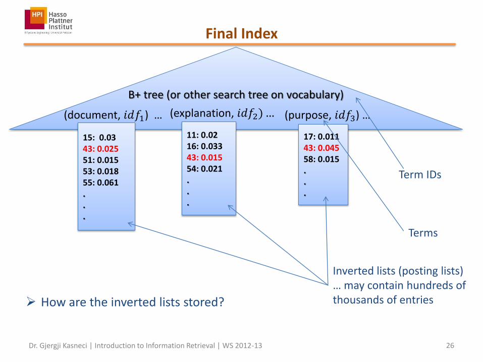
Final Index
Dr. Gjergji Kasneci | Introduction to Information Retrieval | WS 2012-13 26
B+ tree (or other search tree on vocabulary)
(document, 𝑖𝑑𝑓1) …
15: 0.03 43: 0.025 51: 0.015 53: 0.018 55: 0.061 . . .
(explanation, 𝑖𝑑𝑓2) …
11: 0.02 16: 0.033 43: 0.015 54: 0.021 . . .
(purpose, 𝑖𝑑𝑓3) …
17: 0.011 43: 0.045 58: 0.015 . . .
Inverted lists (posting lists) … may contain hundreds of thousands of entries
Term IDs
Terms
How are the inverted lists stored?
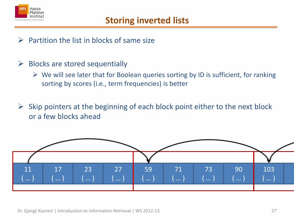
Storing inverted lists
Dr. Gjergji Kasneci | Introduction to Information Retrieval | WS 2012-13 27
11 ( … )
17 ( … )
23 ( … )
27 ( … )
59 ( … )
71 ( … )
73 ( … )
90 ( … )
103 ( … )
Partition the list in blocks of same size
Blocks are stored sequentially
We will see later that for Boolean queries sorting by ID is sufficient, for ranking sorting by scores (i.e., term frequencies) is better
Skip pointers at the beginning of each block point either to the next block or a few blocks ahead
103 ( … )
Compressing inverted lists
Given a Zipf-distribution of terms over the indexed documents, the lengths of the inverted lists will follow the same distribution.
Unbalanced latencies for reading lists of highly varying sizes from disk
Is it possible to mitigate these latencies?
Effective compression needed
Could we apply Ziv-Lempel compression to inverted list entries?
Ziv-Lempel is good for continuous text but not for postings
For inverted lists, gaps between successive doc IDs are encoded
Dr. Gjergji Kasneci | Introduction to Information Retrieval | WS 2012-13 28
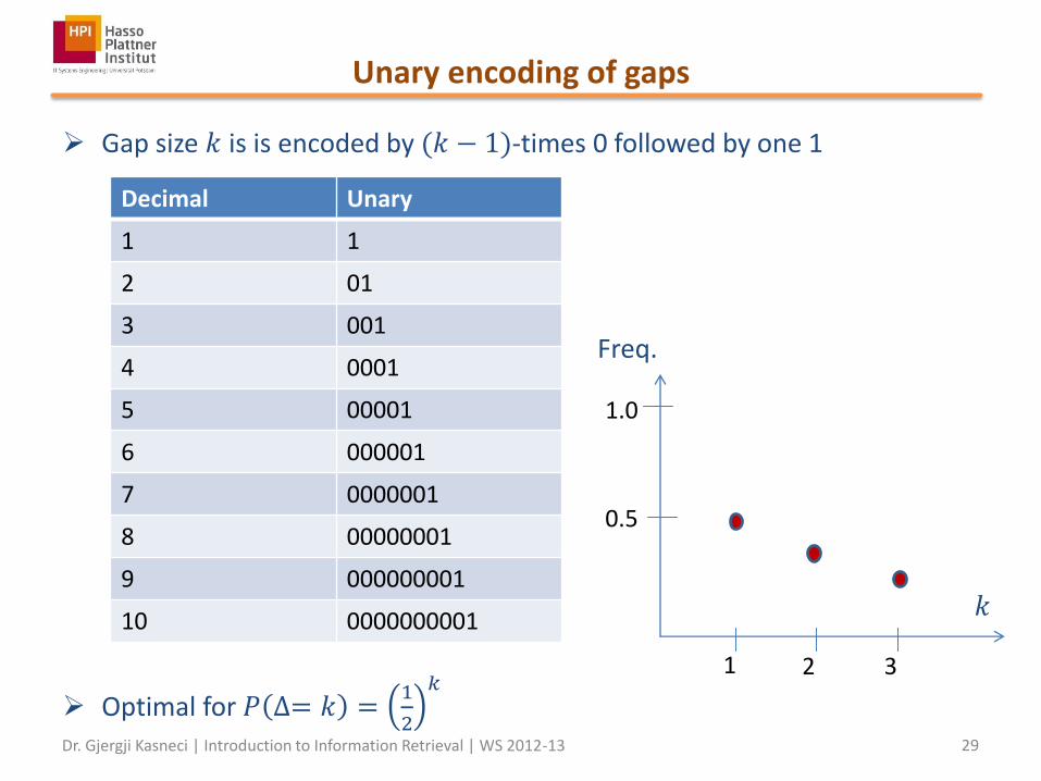
Unary encoding of gaps
Gap size 𝑘 is is encoded by (𝑘 − 1)-times 0 followed by one 1
Optimal for 𝑃 ∆= 𝑘 =1
2
𝑘
Dr. Gjergji Kasneci | Introduction to Information Retrieval | WS 2012-13 29
Decimal Unary
1 1
2 01
3 001
4 0001
5 00001
6 000001
7 0000001
8 00000001
9 000000001
10 0000000001 𝑘
Freq.
1.0
0.5
1 2 3
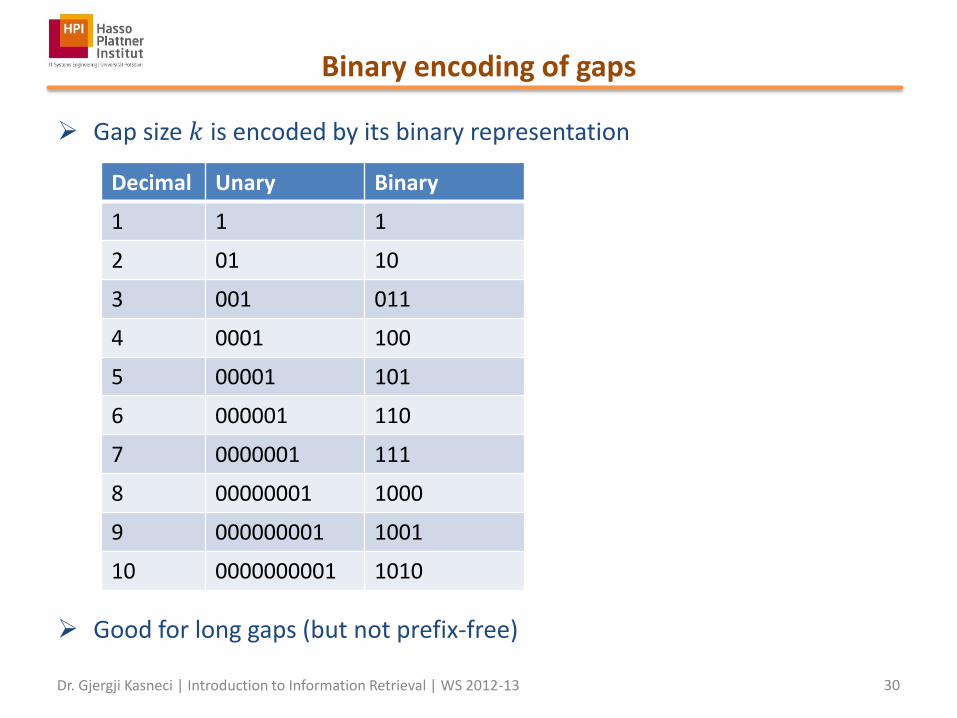
Binary encoding of gaps
Gap size 𝑘 is encoded by its binary representation
Good for long gaps (but not prefix-free)
Dr. Gjergji Kasneci | Introduction to Information Retrieval | WS 2012-13 30
Decimal Unary Binary
1 1 1
2 01 10
3 001 011
4 0001 100
5 00001 101
6 000001 110
7 0000001 111
8 00000001 1000
9 000000001 1001
10 0000000001 1010
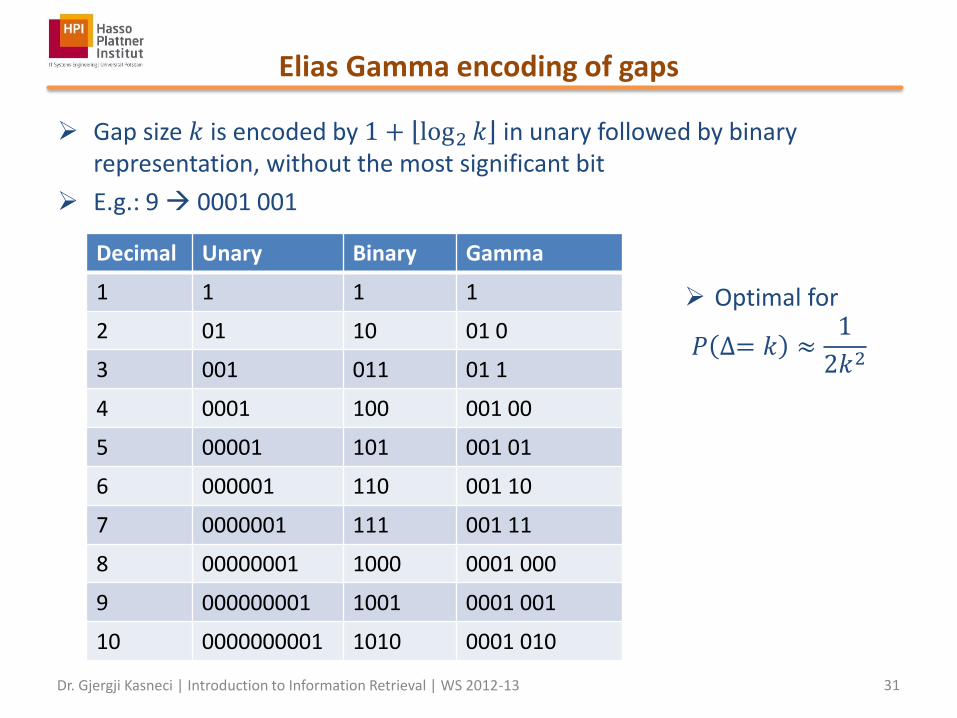
Elias Gamma encoding of gaps
Gap size 𝑘 is encoded by 1 + log2 𝑘 in unary followed by binary representation, without the most significant bit
E.g.: 9 0001 001
Dr. Gjergji Kasneci | Introduction to Information Retrieval | WS 2012-13 31
Decimal Unary Binary Gamma
1 1 1 1
2 01 10 01 0
3 001 011 01 1
4 0001 100 001 00
5 00001 101 001 01
6 000001 110 001 10
7 0000001 111 001 11
8 00000001 1000 0001 000
9 000000001 1001 0001 001
10 0000000001 1010 0001 010
Optimal for
𝑃 ∆= 𝑘 ≈1
2𝑘2
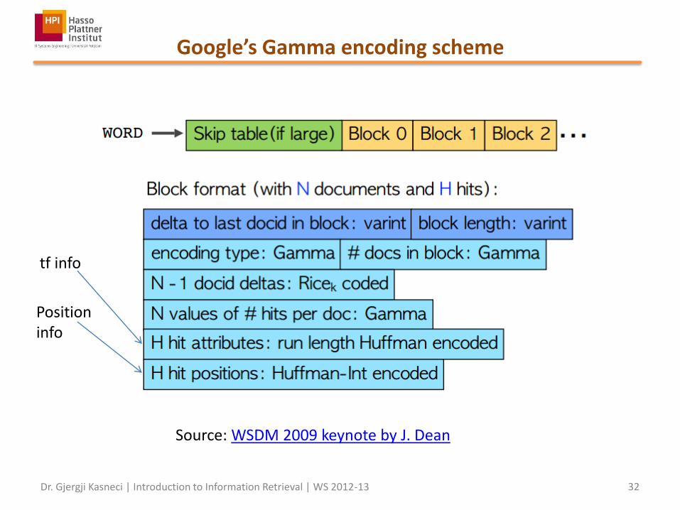
Google’s Gamma encoding scheme
Dr. Gjergji Kasneci | Introduction to Information Retrieval | WS 2012-13 32
Source: WSDM 2009 keynote by J. Dean
tf info
Position info
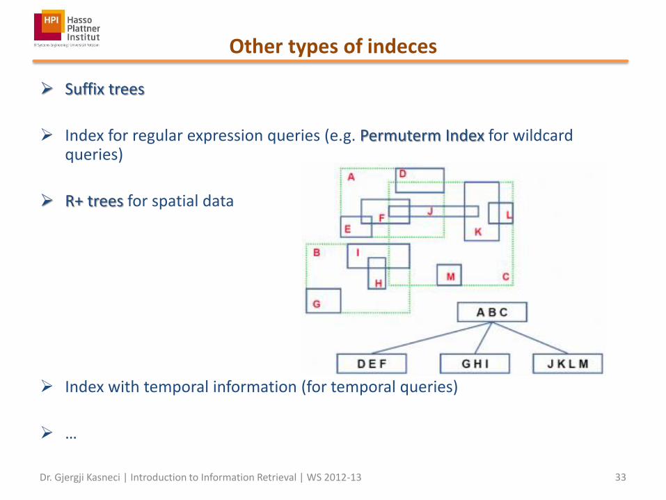
Other types of indeces
Suffix trees
Index for regular expression queries (e.g. Permuterm Index for wildcard queries)
R+ trees for spatial data
Index with temporal information (for temporal queries)
…
Dr. Gjergji Kasneci | Introduction to Information Retrieval | WS 2012-13 33
Summary
Steps to index construction
Sorting docs by terms
vocabulary construction
postings construction
(Parallelization through MapReduce)
Making the vocabulary efficiently searchable with B+ trees
Vocabulary compression (sequential term storage with blocking and prefix replacement)
Prefix trees for maintaining vocabulary of moderate size in main memory
Storing and compressing inverted lists
Equal-size blocks with pointers between subsequent blocks
Gap-based encoding within blocks (Unary, Gamma, Rice, …)
Dr. Gjergji Kasneci | Introduction to Information Retrieval | WS 2012-13 34