Embed Size (px)
Citation preview
INVERTED INDEX COMPRESSION BASEDON TERM AND DOCUMENT IDENTIFIER
REASSIGNMENT
A THESIS
SUBMITTED TO THE DEPARTMENT OF COMPUTER ENGINEERING
AND THE INSTITUTE OF ENGINEERING AND SCIENCE
OF BILKENT UNIVERSITY
IN PARTIAL FULFILLMENT OF THE REQUIREMENTS
FOR THE DEGREE OF
MASTER OF SCIENCE
By
Izzet Cagrı Baykan
September, 2008
I certify that I have read this thesis and that in my opinion it is fully adequate,
in scope and in quality, as a thesis for the degree of Master of Science.
Prof. Dr. Cevdet Aykanat(Advisor)
I certify that I have read this thesis and that in my opinion it is fully adequate,
in scope and in quality, as a thesis for the degree of Master of Science.
Prof. Dr. A. Enis Cetin
I certify that I have read this thesis and that in my opinion it is fully adequate,
in scope and in quality, as a thesis for the degree of Master of Science.
Asst. Prof. Dr. Ilyas Cicekli
Approved for the Institute of Engineering and Science:
Prof. Dr. Mehmet B. BarayDirector of the Institute
ii
ABSTRACT
INVERTED INDEX COMPRESSION BASED ON TERMAND DOCUMENT IDENTIFIER REASSIGNMENT
Izzet Cagrı Baykan
M.S. in Computer Engineering
Supervisor: Prof. Dr. Cevdet Aykanat
September, 2008
Compression of inverted indexes received great attention in recent years. An
inverted index consists of lists of document identifiers, also referred as posting
lists, for each term. Compressing an inverted index reduces the size of the index,
which also improves the query performance due to the reduction on disk access
times.
In recent studies, it is shown that reassigning document identifiers has great
effect in compression of an inverted index. In this work, we propose a novel
technique that reassigns both term and document identifiers of an inverted index
by transforming the matrix representation of the index into a block-diagonal
form, which improves the compression ratio dramatically. We adapted row-net
hypergraph-partitioning model for the transformation into block-diagonal form,
which improves the compression ratio by as much as 50%. To the best of our
knowledge, this method performs more effectively than previous inverted index
compression techniques.
Keywords: inverted index, inverted index compression, block-diagonal form, doc-
ument identifier reassignment, hypergraph partitioning.
iii
OZET
DOKUMAN NUMARALARINI YENIDEN ATAMAYOLU ILE TERS INDEKS SIKISTIRMA
Izzet Cagrı Baykan
Bilgisayar Muhendisligi, Yuksek Lisans
Tez Yoneticisi: Prof. Dr. Cevdet Aykanat
Eylul, 2008
Ters indekslerin sıkıstırılması konusuna son yıllarda oldukca ilgi duyulmustur.
Ters indeks yapısında, her terim icin bir dokuman numara listesi tutulur. Ters
indeksin sıkıstırılması, indeksin boyutunu azaltır ve bu da disk ulasım suresini
azaltacagından dolayı sorgu suresinin azalmasını saglar.
Son calısmalarda, dokuman numaralarının yeniden atanmasının, ters indeks
sıkıstırılmasında oldukca fazla etkili olabilecegi gosterilmistir. Bu calısmamızda,
ters indekslerdeki terim ve dokuman numaralarını, indeksin matris gosterimini
kosegensel blok formuna donusturerek yeniden atamaya yarayan ve boylelikle
sıkıstırma oranında oldukca fazla artıs saglayan bir yontem oneriyoruz. Bu
donusum icin sıkıstırma oranını %50’lere kadar artıran bir ”row-net” hipergraf
parcalama modeli kullanıyoruz. Bildigimiz kadarıyla, bu yontem bundan once
onerilen butun yontemlerden daha etkili sıkıstırma oranları saglamaktadır.
Anahtar sozcukler : Ters indeks, ters indeks sıkıstırma, kosegensel blok formu,
dokuman numarası yeniden atama, hipergraf parcalama.
iv

Acknowledgement
I would like to express my gratitude to my supervisor Prof. Dr. Cevdet Aykanat
for his valuable help, guidance, and trust throughout the study.
I am grateful to Prof. Dr. Cevdet Aykanat, Prof. Dr. Enis Cetin and Asst. Prof.
Dr. Ilyas Cicekli for reading and commenting on my thesis.
I also thank my colleagues Ata, Tayfun, Aylin, Ozlem, Erkan and Enver for
making our office a better place to study. I am grateful to Ata, Tayfun and
Sengor for their valuable help and our great discussions.
I would also like to thank my company, Central Bank of the Republic of Turkey,
for their support and patience throughout the study.
I also want to thank The Scientific and Technological Research Council of Turkey
for their support.
I would like to express my gratitude to my parents for their persistent support
and love.
v
Contents
1 Introduction 1
1.1 Overview . . . . . . . . . . . . . . . . . . . . . . . . . . . . . . . . 1
1.2 Motivation . . . . . . . . . . . . . . . . . . . . . . . . . . . . . . . 2
1.3 Outline of the Thesis . . . . . . . . . . . . . . . . . . . . . . . . . 2
2 Inverted Indexes 4
2.1 Inverted Index Structure & Index Compression . . . . . . . . . . . 4
2.1.1 Related Works on Index Compression . . . . . . . . . . . . 6
2.1.2 Document Identifier Reassignment Problem . . . . . . . . 13
2.1.3 Hypergraph Partitioning . . . . . . . . . . . . . . . . . . . 19
3 Term and Document Id Reassignment 22
4 Implementation & Experimental Results 36
5 Conclusion & Future Work 42
vi
List of Figures
2.1 BDD Encoding - Binary Decision Diagram . . . . . . . . . . . . . 11
3.1 K-way Singly Bordered Block-Diagonal Form (SB Form) . . . . . 23
3.2 Term-Document Matrix Representation of the Sample Inverted Index 25
3.3 Block-Diagonal Forms of a Matrix . . . . . . . . . . . . . . . . . . 26
3.4 Partition Tree Example . . . . . . . . . . . . . . . . . . . . . . . . 27
3.5 Hypergraph Representation of the Sample Inverted Index . . . . . 30
3.6 Matrix Representation After First Bipartitioning . . . . . . . . . . 31
3.7 Hypergraph Representation After First Bipartitioning . . . . . . . 32
3.8 Matrix Representation After Second Bipartitioning . . . . . . . . 33
3.9 Hypergraph Representation After Second Bipartitioning . . . . . . 34
3.10 Partition Trees of Each Bipartitioning Phase . . . . . . . . . . . . 35
4.1 Interrelations of Modules used in Experimental Analysis . . . . . 37
vii
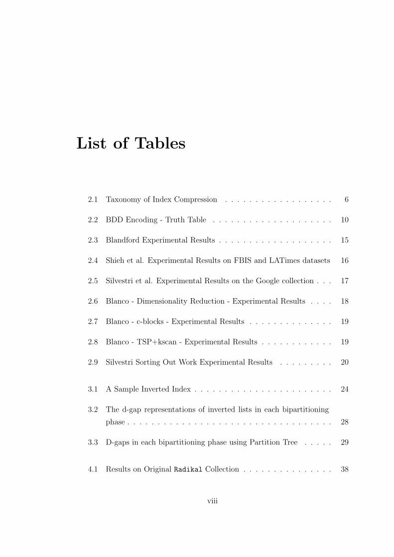
List of Tables
2.1 Taxonomy of Index Compression . . . . . . . . . . . . . . . . . . 6
2.2 BDD Encoding - Truth Table . . . . . . . . . . . . . . . . . . . . 10
2.3 Blandford Experimental Results . . . . . . . . . . . . . . . . . . . 15
2.4 Shieh et al. Experimental Results on FBIS and LATimes datasets 16
2.5 Silvestri et al. Experimental Results on the Google collection . . . 17
2.6 Blanco - Dimensionality Reduction - Experimental Results . . . . 18
2.7 Blanco - c-blocks - Experimental Results . . . . . . . . . . . . . . 19
2.8 Blanco - TSP+kscan - Experimental Results . . . . . . . . . . . . 19
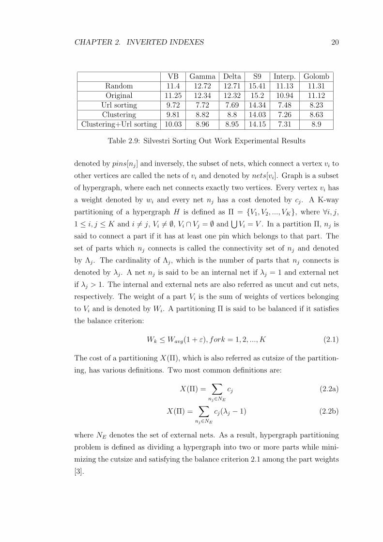
2.9 Silvestri Sorting Out Work Experimental Results . . . . . . . . . 20
3.1 A Sample Inverted Index . . . . . . . . . . . . . . . . . . . . . . . 24
3.2 The d-gap representations of inverted lists in each bipartitioning
phase . . . . . . . . . . . . . . . . . . . . . . . . . . . . . . . . . . 28
3.3 D-gaps in each bipartitioning phase using Partition Tree . . . . . 29
4.1 Results on Original Radikal Collection . . . . . . . . . . . . . . . 38
viii

LIST OF TABLES ix
4.2 Results on Randomized Radikal Collection . . . . . . . . . . . . . 38
4.3 Results on Original Google-plus Collection . . . . . . . . . . . . 39
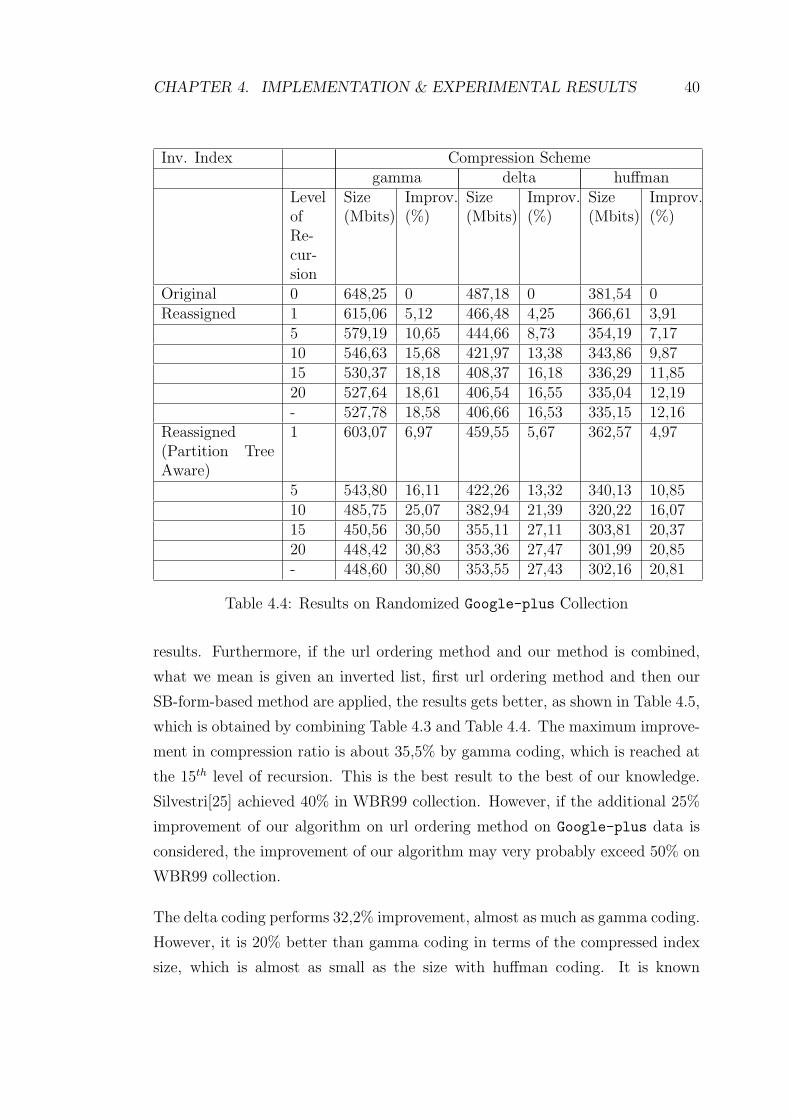
4.4 Results on Randomized Google-plus Collection . . . . . . . . . . 40
4.5 Results combination of Url Ordering and Our Technique . . . . . 41
Chapter 1
Introduction
The available data on the Internet have been growing astronomically. Web Search
Engines (WSE) have also been providing more eligible techniques since it is get-
ting harder to find what you are looking for with the increase in the available
data. This whole data on the Internet would be nothing but garbage without
good searching facilities.
1.1 Overview
A WSE mainly consists of three distinct modules. The Crawler gathers the data
available and stores it in a huge repository. The Indexer constructs an index
by abstracting the data in the repository in order to provide fast access to the
data content. Finally, the searcher accepts queries and returns references to the
documents that matches best to the query. The most commonly used index
structure is Inverted Index, which is also referred as Inverted File, which, for
each term, keeps a list of document identifiers that the term appears.
1
CHAPTER 1. INTRODUCTION 2
1.2 Motivation
The size of an inverted index can vary from 50% to 100% of the size of data in
the repository [31], which makes the compression of inverted indexes a critical
issue. Compression of inverted indexes decreases not only the space required to
store the index but also the query response time due to the reduction in disk
access times. Different compression schemes are proposed in order to compress
an inverted index. These schemes include the well-known global coding schemes
such as elias gamma, elias delta and variable coding as well as those, which were
proposed specifically for inverted indexes. The most common technique that is
used together with these schemes is the d-gap value representation, in which
the document identifiers in each posting list is sorted in increasing order and
the successive differences are stored instead of the identifiers themselves. In this
representation, the numbers in posting lists becomes smaller, which results in
better compression ratio.
It can intuitively be observed that any reassignment of the document iden-
tifiers will effect the compression ratio due to the change in the d-gap values,
either positively or negatively. Clustering the documents and assigning closer
identifiers to documents that are in the same cluster will definitely increase the
compression ratio. We propose a novel technique that exploits the one-to-one
correspondance between inverted indexes and their matrix representations, and
uses the tranformation of the matrices into singly bordered block-diagonal form
[4]. To the best of our knowledge, this method performs more effectively than
previously proposed techniques.
1.3 Outline of the Thesis
Chapter 2 gives a short explanation of the compression schemes that are com-
monly used in the compression of inverted indexes as well as schemes that are
recently proposed, and it also presents a couple of categorizations over these
CHAPTER 1. INTRODUCTION 3
schemes. The chapter also includes previous works on document identifier re-
assignment along with their performance analyses. The final part of Chapter 2
presents a brief introduction to the hypergraph-partitioning concept used in this
work. Chapter 3 presents the model in details: The one-to-one mapping between
an inverted index and its matrix representation, how a matrix is tranformed into
its singly bordered block-diagonal form, how a matrix can be represented by a
hypergraph, etc. After the experimental results of the model in Chapter 4, final
chapter of the thesis provides a summary of this work and suggestions for future
work.
Chapter 2
Inverted Indexes
Due to the astronomic increase on the available data on the Internet, the speed
and the accuracy of Web Search Engines (WSE) have become much more impor-
tant than it has ever been. Basically, what is performed by a WSE is selecting
up a subset of the available documents based on a user’s query, which may be
composed of terms or phrases. In order to reach acceptable response times, an
indexing mechanism, usually the Inverted Index data structure, is used.
2.1 Inverted Index Structure & Index Compres-
sion
An Inverted index is a commonly used data structure in efficient text search. An
inverted index of a set of documents consists of two elements: the lexicon and the
posting list. Lexicon is the list of terms, each appearing in at least one of the docu-
ments in the collection. Each term in the lexicon has a list of postings, which rep-
resents information about the occurrence of the term. In a boolean inverted index,
a posting represents only a document identifier. Let ti be a term in the lexicon and
pi =< fti ; dti1 , dti2 , ..., dfti> be its posting list. Here ft is the frequency of ti in the
document set, which is the number of documents that ti appears in and following
4
CHAPTER 2. INVERTED INDEXES 5
dtij ’s are the identifiers of those documents. For example, pi =< 4; 2, 7, 15, 32 >
shows that ti appears in four documents, which are identified by 2,7,15,32. In
a ranked inverted index, in addition to a boolean inverted index, a posting list
pi =< fti ; (dti1 , w(dti1 , ti)), (dti2 , w(dti2 , ti)), ..., (dfti, w(dfti
, ti)) > represents also
w(dtij , ti)’s, which is the frequency of the term ti in document dtij . For example,
pi =< 4; < 2, 3 >,< 7, 1 >,< 15, 2 >,< 32, 7 >> shows that ti appears three
times in document 2, once in document 7, twice in document 15, seven times in
document 32 and totally in 4 different documents. In some cases, the positions
of the term in the document are also stored in the index. Since our work focuses
on compressing document identifiers, we will use the term “inverted index“ for
“boolean inverted index“, but we will also show that it also applies to ranked
inverted indexes.
The size of an inverted index can vary from 50% to 100% of the size of the original
text [31]. This size can grow according to the granularity of an index. Here the
granularity of the index defines the level of detail stored in the index. In a coarse-
grain index, a single pointer or identifier can be used for a group of documents,
whereas in a moderate-grain index, an identifier for each document can be used,
and in a fine-grain index the paragraph or the sentence number, or even the
exact position of the term can be stored in addition to the document identifier
[31]. Therefore, compression of the inverted index for huge document collections
is crucial. Compression of the inverted index also affects the query evaluation
time because when a query is submitted, the posting lists of each query term is
retrieved from the disk and retrieving compressed posting lists will require less
time because of their smaller size. A common strategy for compression of inverted
indexes is the d-gap representation of posting lists. The d-gap representation of
a posting list is obtained by sorting document id’s in increasing order and for
each document id, storing the successive differences. More precisely, instead of
storing < 4; 2, 7, 15, 32 >, < 4; 2, 7− 2, 15− 7, 32− 15 > which is < 4; 2, 5, 8, 17 >
is stored. Obviously, the first id is stored as is.
CHAPTER 2. INVERTED INDEXES 6
2.1.1 Related Works on Index Compression
Research on compression of inverted indexes can be grouped into two categories:
global codes, in which all the posting lists are compressed with the same com-
pression scheme and local codes, in which the compression scheme is modified
for each posting list. Another categorization can be done according to whether
they exploit clustering property or not. Lastly, the compression of indexes can be
grouped by whether they favor compression ratio or decompression performance.
According to these three categories, a classification of the research on this area
is shown in Table 2.1.
With Clustering W/out ClusteringGlobal Local Global Local
Comp. RatioGamma Interpolative, Golomb GolombDelta k-base gamma/k-
flat binary,g-binary g-binary
d-gap pattern sigma BDD
Decoding Perf.Unary Word-Aligned
Binary,BDD
Variable Byte Fixed Binary,Hybrid bitvector
Table 2.1: Taxonomy of Index Compression
Unary coding represents a positive integer x by (x-1) zeros followed by a one [13].
For example, the unary coding of 4 is 0001. As anyone can notice, encoding with
unary code is expensive except very small numbers. In a 32-bit integer system,
encoding numbers larger than 32 with unary codes is not meaningful. However,
unary coding is used effectively in some other encoding schemes such as gamma
coding.
Elias Gamma coding is a little more complicated than unary coding. In gamma
coding, a positive integer x is firstly written as x = 2⌊log x⌋ + (x − 2⌊log x⌋). After
that, 1+⌊log x⌋ is encoded by unary codes and x−2⌊log x⌋ is encoded by ⌊log x⌋ bits
binary representation [13]. For example, let x = 25, ⌊log 25⌋ = 4 and 25−2⌊log 25⌋
= 9. Unary encoding of 1+⌊log 25⌋ = 1+4 = 5 is 00001 and 4 bit representation of
9 is 1001. So, gamma encoding of x=25 is 000011001. Gamma coding is efficient
CHAPTER 2. INVERTED INDEXES 7
for small integers.
Elias Delta coding is very much like gamma coding. A positive integer x is
firstly written as x = 2⌊log x⌋ + (x − 2⌊log x⌋). After that 1 + ⌊log x⌋ is encoded
by gamma codes instead of unary codes and the remaining x− 2⌊log x⌋ is encoded
by ⌊log x⌋ bits binary representation [13]. On the contrary of gamma encoding,
delta encoding is efficient for large integers.
Golomb coding is like elias coding. A positive integer x is firstly divided into two
parts. Unlike elias coding, this division is performed based on some parameter
b. First part q+1 is encoded by unary codes, where q= ⌊(x− 1)/b⌋ and then the
remainder r=x-qb-1 is encoded by ⌊log b⌋ or ⌈log b⌉ bits binary representation.
More precisely, when r < p the number is encoded as q+1 in unary code and r in
⌊log b⌋ bits binary code. Otherwise, it is encoded as q+1 in unary code and r+p in
⌈log b⌉ bits binary code, where p=2⌊log b⌋+1−b [27]. For example, let x=9 and b=3.
Calculations lead to q=2, r=2 and p=1. Then q+1 is encoded by unary code and
r+p is encoded in ⌈log b⌉ bits binary code. So the encoded string is 00111. The
way of choosing b is critical. Global or Local Bernoulli Model can be used to
choose b effectively. Global Bernoulli method uses the assumption that terms are
uniformly distributed among all documents, which makes the probability of a ran-
domly selected term to appear in a randomly selected document be p = f/(N ·n),
where N is number of documents and n is the number of terms. Local Bernoulli
method, uses a slightly different assumption that each selected term is uniformly
distributed among all documents, which makes the probability of a selected term
appear in a randomly selected document be p = f/N . In both methods, b is
chosen as b = ⌈ log(2−p)− log(1−p)
⌉ [21]. The major difference in Local Bernoulli method
is that for each inverted list, a different b value is used. In addition, localized
Golomb code achieves better compression by using the local information of each
posting list[27]. However, it does not adapt well to the clustering property of
inverted indexes [1]. In recent years, some techniques are proposed, which use
clustering property to enhance the compressibility. Interpolative coding is such
an example, which outperforms Golomb coding for typical document sets [20].
CHAPTER 2. INVERTED INDEXES 8
Interpolative coding is proposed by Moffat et al. in 2000 [20]. A monotoni-
cally increasing list of positive integers can be encoded by the idea that if the
even indexed numbers are known, then the odd indexed can be encoded with
predictable-length binary codes. For example, let pi0 =< 5; 2, 7, 10, 13, 15 > be
a posting list in a collection of 18 documents. If pi1 =< 2; 7, 13 > is already
encoded, then the ranges of the first, third and fifth numbers are in the ranges
(1,6), (8,12) and (14,17) inclusive and can be encoded by (3,3,2)-bits binary rep-
resentations, respectively. This idea is improved by the same method used in
encoding of the second part in Golomb code, such as for some x be in the range
(lo, hi), some values of x can be encoded by ⌊log(hi − lo + 1)⌋ bits instead of
⌈log(hi − lo + 1)⌉ bits.
The technique proposed by Chen et al. [11] also uses cluster property of in-
verted indexes, which is inspired by the idea that terms in a document collec-
tion are not uniformly distributed. In a clustered inverted index, many fre-
quent d-gap patterns may exist. Every pattern that exist multiple times in
the document is assigned a pattern-id. After this operation, any posting list
pi =< fti ; dti1 , dti2 , ..., dfti> is transformed to p′i =< f ′
ti; gti1 , gti2 , ..., gfti
> where
gi is either a pattern-id or a d-gap. In order to decide whether a gi is a d-
gap or pattern-id, for every inverted list, number of patterns and their positions
are encoded by gamma code. After that, d-gap’s are encoded by gamma code,
whereas the pattern-id’s are encoded with Huffman code. For example, let pi =<
9; 5, 2, 3, 3, 5, 4, 6, 4, 4 > be a posting list and si =< 5, 2, 3 > andsj =< 5, 4, 6, 4 >
be two d-gap sequence patterns, which are assigned pattern-ids 4 and 2, respec-
tively. Then the transformed inverted index is < 4; 4, 3, 2, 4 > with an additional
information < 2; 1, 3 > (number of pattern-ids and their positions) encoded by
gamma code.
Mixed k-base Gamma/k-flat Binary Code [12] is another technique, which uses
the cluster property. In this model, for an inverted list < f ; d1, d2, ..., df >,
where f is the document frequency of the term, di is the ith document id in the
inverted list; any segment < di, di+1, ..., dj >, where i ≤ j, every id in the seg-
ment is less than 2k for some predetermined k, and no adjacent id is less than
CHAPTER 2. INVERTED INDEXES 9
2k is considered to be a cluster and encoded by different scheme. More pre-
cisely, a posting list pi =< fti ; dti1 , dti2 , ..., dtifti> is transformed to its cluster
representation as < f ′ti; gti1 , gti2 , ..., gtifti
′ >, where gtij is either a cluster or a non-
clustered d-gap. After transformation, every non-clustered d-gap x is encoded
as x/2k with gamma code and the remainder with k-bit binary representation.
The d-gaps in the clusters are encoded by k-bit binary representation. For ex-
ample, let k=2 and p =< 17; 6, 15, 5, 4, 2, 3, 2, 1, 25, 32, 21, 7, 3, 2, 5, 4, 3 > be an
inverted list. Then the transformation leads to the cluster representation p as
p′ =< 13; 6, 15, 5, 4, (2, 3, 2, 1), 25, 32, 21, 7, (3, 2), 5, 4, (3) >. Every non-clustered
id x is encoded by x/4 with gamma code and the remainder r with two bit rep-
resentation, for instance 21 is encoded by 5 with gamma code and 1 with two bit
binary representation; and every clustered id 2 is encoded with two bit binary
representation. Here the major issue is how to determine the start and end points
of the clusters. Two categories of methods are suggested, one with a header which
stores the start position and the size of each cluster, the other one which stores
dedicated bits at the start and end points of each cluster.
In Binary decision diagram encoding [18], as revealed by the name, a data struc-
ture called binary decision diagram (BDD) is used. A BDD is an acyclic, directed
graph, which has two types of nodes: decision nodes and terminal nodes. A de-
cision node stores a variable and for each two possible values (0 or 1), it has an
outgoing edge that connects it to either a decision or terminal node. A terminal
node stores a value (0 or 1) and does not have any outgoing edges. Given a combi-
nation of values of the variables, a traverse from the root node leads to a terminal
node, which is so called the result. Constructing the BDD of an inverted list is
performed as follows: All the bits from least significant to most significant is as-
signed to a variable ij, where j=0,1,..,⌊log N⌋ and N is the number of documents
in the document collection. After that, the truth table of ⌊log N⌋+ 1 variables is
generated. This truth table should result true if that document id exists in the
list and false otherwise. For example, let pi =< 8 : 0, 2, 5, 6, 8, 11, 12, 14 > be a
posting list. The truth table and corresponding BDD are shown in Table 2.2 and
Figure 2.1, respectively. The binary representation of a BDD consists of two parts.
The types of the nodes in breadth-first traversal order are stored in the first part
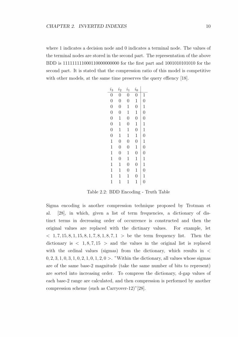
CHAPTER 2. INVERTED INDEXES 10
where 1 indicates a decision node and 0 indicates a terminal node. The values of
the terminal nodes are stored in the second part. The representation of the above
BDD is 111111111000110000000000 for the first part and 1001010101010 for the
second part. It is stated that the compression ratio of this model is competitive
with other models, at the same time preserves the query effiency [18].
i3 i2 i1 i00 0 0 0 10 0 0 1 00 0 1 0 10 0 1 1 00 1 0 0 00 1 0 1 10 1 1 0 10 1 1 1 01 0 0 0 11 0 0 1 01 0 1 0 01 0 1 1 11 1 0 0 11 1 0 1 01 1 1 0 11 1 1 1 0
Table 2.2: BDD Encoding - Truth Table
Sigma encoding is another compression technique proposed by Trotman et
al. [28], in which, given a list of term frequencies, a dictionary of dis-
tinct terms in decreasing order of occurrence is constructed and then the
original values are replaced with the dictinary values. For example, let
< 1, 7, 15, 8, 1, 15, 8, 1, 7, 8, 1, 8, 7, 1 > be the term frequency list. Then the
dictionary is < 1, 8, 7, 15 > and the values in the original list is replaced
with the ordinal values (sigmas) from the dictionary, which results in <
0, 2, 3, 1, 0, 3, 1, 0, 2, 1, 0, 1, 2, 0 >. ”Within the dictionary, all values whose sigmas
are of the same base-2 magnitude (take the same number of bits to represent)
are sorted into increasing order. To compress the dictionary, d-gap values of
each base-2 range are calculated, and then compression is performed by another
compression scheme (such as Carryover-12)”[28].
CHAPTER 2. INVERTED INDEXES 11
Figure 2.1: BDD Encoding - Binary Decision Diagram
Beside these compression schemes, some hybrid schemes are also proposed. One of
them is Evangilidis’ g-binary method [21]. G-binary is a hybrid between Golomb
code and binary representation of numbers. For a positive number x, the encoding
consists of two parts. First part is the minimum number of bits needed for the
representation of x, which is encoded by Golomb code and the second part is
the binary representation of x except the most significant bit, which is always
1. Total number of bits required for the encoding of x by g-binary is at most
⌊⌊log(x)⌋/b⌋ + 1 + ⌈log(b)⌉ + ⌊log(x)⌋, where b is the parameter for Golomb
coding.
Another hybrid scheme is hybrid bitvector scheme, which is a hybrid between
bitvector code and byte code [19]. For an inverted list of a document collection
with N documents, bitvector code is a list of N numbers < b1, b2, ..., bN >, where
bi=0 or 1 indicating whether the term exists in documenti. The inverted list of
a term with document frequency f > N/8 occupies less space if it is compressed
CHAPTER 2. INVERTED INDEXES 12
by bitvector code than byte code, since byte code will cost at least 8f bits. One
major difference between hybrid bitvector and the previous encoding schemes
is that the primary objective of hybrid bitvector is the decoding performance,
whereas compression ratio it is for the previous ones’. Variable byte code, word
aligned binary code and fixed binary code are the significant compression schemes,
whose primary objective are also decoding performance.
In variable byte code, an integer x is encoded by one or more bytes, The most
significant bit of every byte is used as a flag, where a 1 represents the last byte
and a 0 represents that there are more bytes. The remaining seven bits of each
byte are used for the data. For example, 260 is encoded as 00000010 10000100.
A slightly different implementation suggests that if a number x is represented by
2 bytes, then it means that it cannot be represented by 1 byte. So, x ≥ 27. As a
result, encoding x as (x− 27) in 2 bytes will be more logical because by this way
a number x, where 27 ≤ x < 214 + 27 can be encoded in 2 bytes. More generally,
a number x, where∑
27(y−1) ≤ x <∑
27y can be represented by y bytes.
Word aligned binary code is a hybrid between bit-aligned and byte-aligned codes
[2]. It is not as good as the best models in terms of compression rate but it
has exceptionally low decoding time. The idea is to assign maximum number of
integers into each word. The integers in different words can be represented by
different number of bits, but those in the same word is represented with same
number of bits. Three variants of this approach is stated. In Simple-9 scheme,
every first four bits are used as selectors, and the remaining 28 bits are used to
store the data. Data can be either one 28-bits, two 14-bits, three 9-bits, four
7-bits, five 5-bits, seven 4-bits, nine 3-bits, fourteen 2-bits or twenty eight 1-bit
data. The selector bits have a value from 1 to 9 respectively. In Relative-10
scheme, the number of selector bits is reduced to 2 and the remaining bits are
used to store data. However, number of combinations of the data increased. So,
2-bits selector bits are not enough to represent every combination. Instead, it is
used as follows: Each combination has an identity number from 1 to 10. For any
word in the sequence, let r be the identity number of the combination used in
the previous word, the selector bits indicate either one of (r − 1)th, rth, (r + 1)th
or last identity numbers. If previous selector indicates the last identity number,
CHAPTER 2. INVERTED INDEXES 13
then the fourth of the previous choices becomes the first identity number. In
some combinations of the Relative-10 scheme, there are two unused bits at the
end. In Carryover-12, those bits are used to be the selector of the next word. If
the selector of a word is placed in the previous word, then 32 bits are used to
store the data. Otherwise, as in Relative-10 30 bits are used. Whenever a word
can store the selector of the next one, it does.
In Fixed Binary codewords, each posting list is splitted into multi-
ple posting lists, in which every document identifier is represented with
the same number of bits. (w, s; d1, d2, ..., ds) indicates that this split
has s documents each represented by w-bit binary code. For exam-
ple, let pi =< 15; 10, 5, 14, 8, 35, 25, 32, 26, 7, 15, 18, 13, 20, 25, 30 >, then <
15; (4, 4; 10, 5, 14, 8), (6, 4; 35, 25, 32, 26), (5, 7; 7, 15, 18, 13, 20, 25, 30) > is an ex-
ample split. The number of bits used for every identifier in a split is determined by
the minimum number of bits required for the representation of the maximum val-
ued identifier. For example, the maximum valued identifier in (6, 4; 35, 25, 32, 26)
is 35, and it requires at least 6 bits for binary representation. So, every iden-
tifier is encoded by 6 bits. This simplest case of this model requires five bits
for representing the length of each identifier, and additional bits for representing
the number of postings considering that the document collection can contain as
many as 230 documents. To reduce number of selector bits, a technique similar
to the one used in word aligned binary codes is adapted. In this technique, there
are 16 different possibilities for (w,s) values which are relative to the previous
(w, s) value. There are three predetermined s values: s1, s2ands3. For example,
if the value of the selector bits is 5 (among the 16 possibilities), then (wi+1, si+1)
is (wi − 1, s3). In this case number of bits required to represent both w and s is
reduced to 4.
2.1.2 Document Identifier Reassignment Problem
As mentioned, one of the categorization of index compression schemes is whether
a scheme exploits clustering property of inverted indexes. Among these schemes,
there are continuing research on improving the clustering property of inverted
CHAPTER 2. INVERTED INDEXES 14
indexes, by this way enhancing better compression.
2.1.2.1 Problem Definition
For a term ti, if it appears in a document dj in a context ck; then it is likely to
happen that ti appears in some other documents in the same context. For this
reason, assigning closer identifiers to documents in similar contexts will reduce
the d-gap values, which will result in better compression. Consequently, the doc-
ument identifier reassignment problem can be defined as mapping each document
identifier into a different identifier (as well as the same identifier) in order to
improve the compression ratio.
2.1.2.2 Related Works on Document Identifier Reassignment
The Document Identifier Reassignment is a new approach to improve the clus-
tering property of inverted indexes. The first work was proposed by Blandford
et al. [8] in 2002. In this technique, firstly Document Similarity Graph of the
inverted index is built. Before giving the details of the graph, let us define what
document similarity is. Let Di = {ti,1, ti,2, ..., ti,m} be a document in the collec-
tion, where m is the number of terms and ti,j = 0, 1 indicates whether tj appears
in Di. Document similarity is between two documents is calculated based on some
metric on the common terms of these documents. In Blandford’s work, the cosine
measure is used to determine the pairwise similarity of documents such as Di and
Dj being two documents in the collection, Si,j = cos(Di, Dj) =Di·Dj√
(Di·Di)(Dj ·Dj).
Building document similarity graph starts with the calculation of pairwise simi-
larities of all documents. For each document Di, a vertex vi is added to the graph.
After that, for each document Di, an edge (i, j) is added to the graph only if the
documents Di and Dj have at least one common term which is not a stopword,
where j = 1..|D|, j 6= i. Stopwords are the terms like ”the”, ”a”, ”any”, whose
frequency in the collection is more than a threshold value and can be ommitted
since they are not significant in query results and they do increase complexity
of calculations. After building the graph, a hierarchical clustering is applied. At
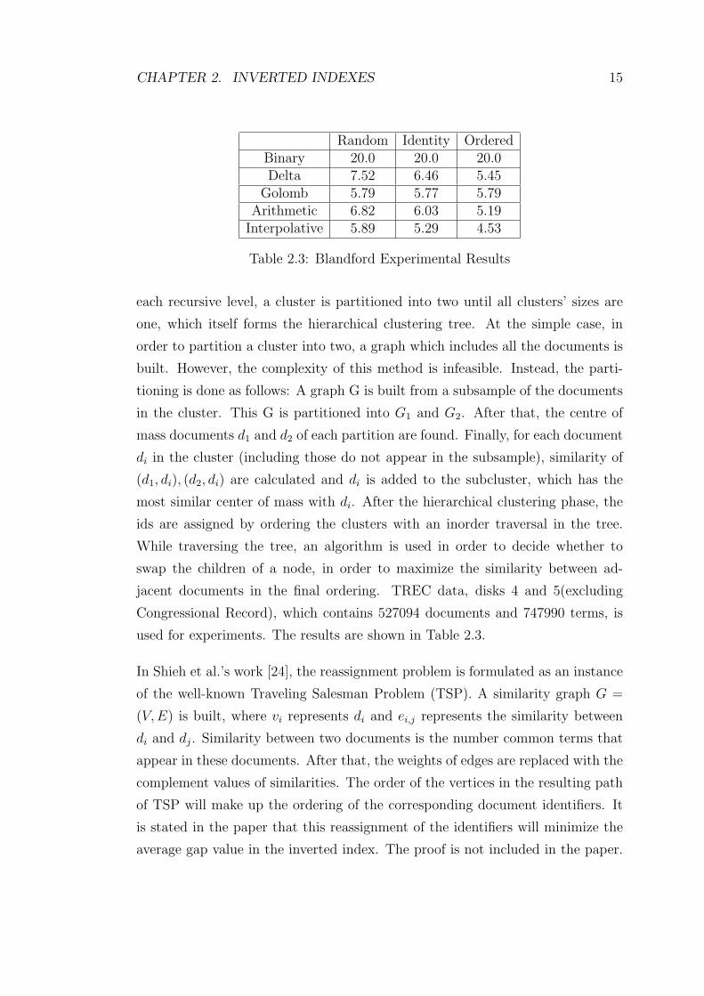
CHAPTER 2. INVERTED INDEXES 15
Random Identity OrderedBinary 20.0 20.0 20.0Delta 7.52 6.46 5.45
Golomb 5.79 5.77 5.79Arithmetic 6.82 6.03 5.19
Interpolative 5.89 5.29 4.53
Table 2.3: Blandford Experimental Results
each recursive level, a cluster is partitioned into two until all clusters’ sizes are
one, which itself forms the hierarchical clustering tree. At the simple case, in
order to partition a cluster into two, a graph which includes all the documents is
built. However, the complexity of this method is infeasible. Instead, the parti-
tioning is done as follows: A graph G is built from a subsample of the documents
in the cluster. This G is partitioned into G1 and G2. After that, the centre of
mass documents d1 and d2 of each partition are found. Finally, for each document
di in the cluster (including those do not appear in the subsample), similarity of
(d1, di), (d2, di) are calculated and di is added to the subcluster, which has the
most similar center of mass with di. After the hierarchical clustering phase, the
ids are assigned by ordering the clusters with an inorder traversal in the tree.
While traversing the tree, an algorithm is used in order to decide whether to
swap the children of a node, in order to maximize the similarity between ad-
jacent documents in the final ordering. TREC data, disks 4 and 5(excluding
Congressional Record), which contains 527094 documents and 747990 terms, is
used for experiments. The results are shown in Table 2.3.
In Shieh et al.’s work [24], the reassignment problem is formulated as an instance
of the well-known Traveling Salesman Problem (TSP). A similarity graph G =
(V,E) is built, where vi represents di and ei,j represents the similarity between
di and dj. Similarity between two documents is the number common terms that
appear in these documents. After that, the weights of edges are replaced with the
complement values of similarities. The order of the vertices in the resulting path
of TSP will make up the ordering of the corresponding document identifiers. It
is stated in the paper that this reassignment of the identifiers will minimize the
average gap value in the inverted index. The proof is not included in the paper.
CHAPTER 2. INVERTED INDEXES 16
Besides, it is clear that minimum average gap value does not necessarily lead to
the minimum compression ratio. Since the TSP is an NP-Complete problem, a
couple of heuristics are adapted to the implementation of this work. FBIS and
LATimes datasets are used for experiments. The best results are observed with
delta encoding and the heuristic called Greedy-NN. The results are shown in
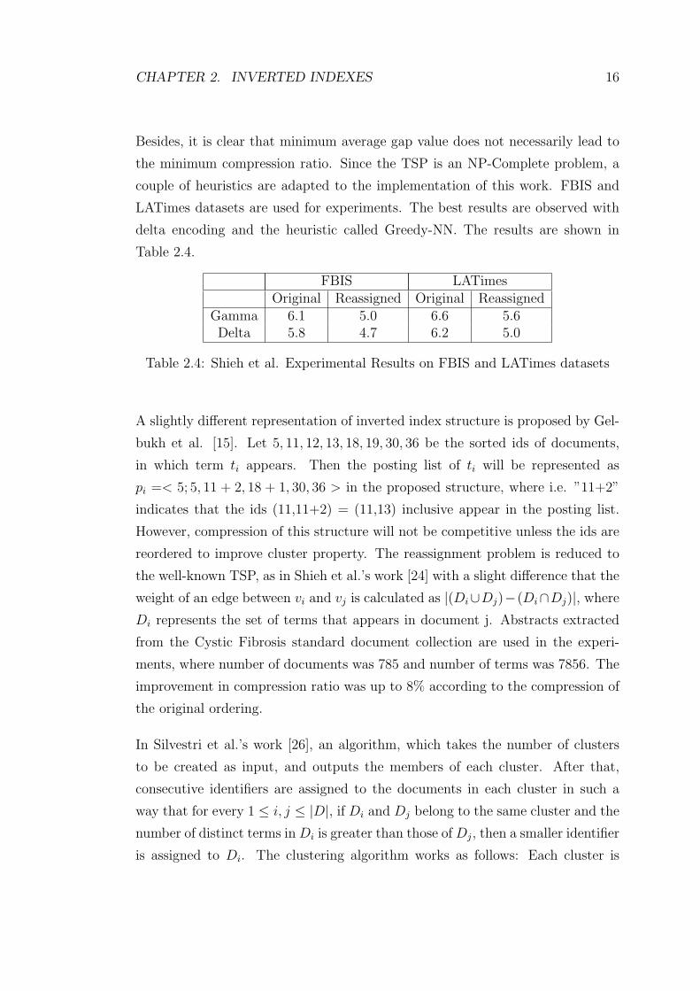
Table 2.4.
FBIS LATimesOriginal Reassigned Original Reassigned
Gamma 6.1 5.0 6.6 5.6Delta 5.8 4.7 6.2 5.0
Table 2.4: Shieh et al. Experimental Results on FBIS and LATimes datasets
A slightly different representation of inverted index structure is proposed by Gel-
bukh et al. [15]. Let 5, 11, 12, 13, 18, 19, 30, 36 be the sorted ids of documents,
in which term ti appears. Then the posting list of ti will be represented as
pi =< 5; 5, 11 + 2, 18 + 1, 30, 36 > in the proposed structure, where i.e. ”11+2”
indicates that the ids (11,11+2) = (11,13) inclusive appear in the posting list.
However, compression of this structure will not be competitive unless the ids are
reordered to improve cluster property. The reassignment problem is reduced to
the well-known TSP, as in Shieh et al.’s work [24] with a slight difference that the
weight of an edge between vi and vj is calculated as |(Di∪Dj)−(Di∩Dj)|, where
Di represents the set of terms that appears in document j. Abstracts extracted
from the Cystic Fibrosis standard document collection are used in the experi-
ments, where number of documents was 785 and number of terms was 7856. The
improvement in compression ratio was up to 8% according to the compression of
the original ordering.
In Silvestri et al.’s work [26], an algorithm, which takes the number of clusters
to be created as input, and outputs the members of each cluster. After that,
consecutive identifiers are assigned to the documents in each cluster in such a
way that for every 1 ≤ i, j ≤ |D|, if Di and Dj belong to the same cluster and the
number of distinct terms in Di is greater than those of Dj, then a smaller identifier
is assigned to Di. The clustering algorithm works as follows: Each cluster is
CHAPTER 2. INVERTED INDEXES 17
created successively, one after the other. At each clustering, the longest document
among the documents which are not already assigned to a cluster is selected.
After that, (|D|/k) − 1 documents that are most similar to the that document
are selected, in which these |D|/k documents together form a new cluster. Jaccard
measure is used for similarity metric, where similarity between two documents
Di and Dj is calculated by|Di∩Dj |
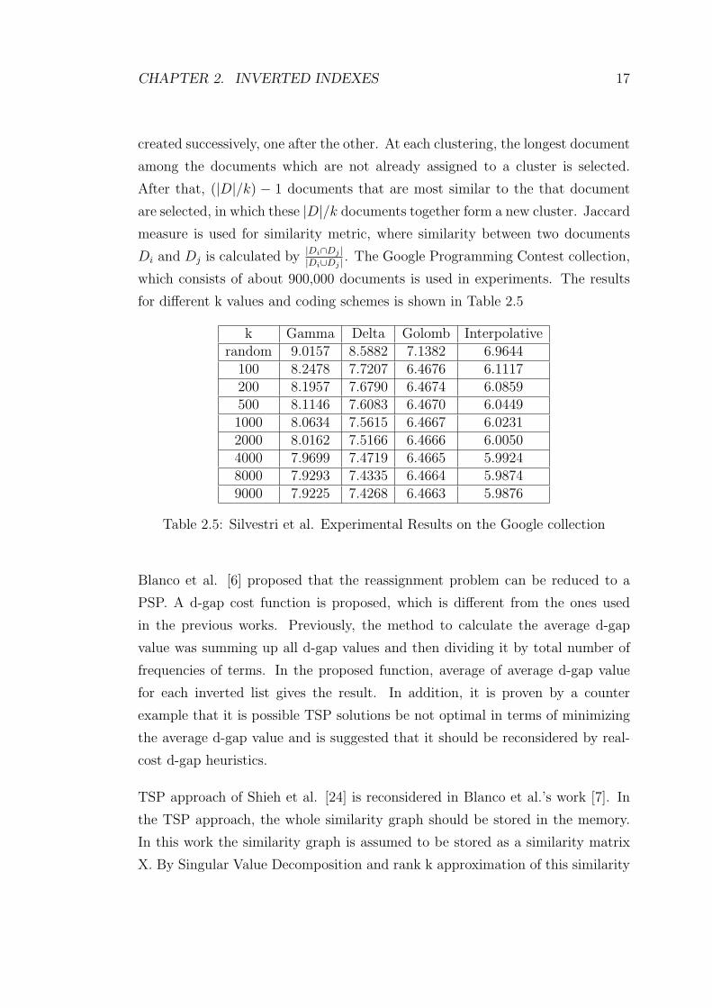
|Di∪Dj |. The Google Programming Contest collection,
which consists of about 900,000 documents is used in experiments. The results
for different k values and coding schemes is shown in Table 2.5
k Gamma Delta Golomb Interpolativerandom 9.0157 8.5882 7.1382 6.9644
100 8.2478 7.7207 6.4676 6.1117200 8.1957 7.6790 6.4674 6.0859500 8.1146 7.6083 6.4670 6.04491000 8.0634 7.5615 6.4667 6.02312000 8.0162 7.5166 6.4666 6.00504000 7.9699 7.4719 6.4665 5.99248000 7.9293 7.4335 6.4664 5.98749000 7.9225 7.4268 6.4663 5.9876
Table 2.5: Silvestri et al. Experimental Results on the Google collection
Blanco et al. [6] proposed that the reassignment problem can be reduced to a
PSP. A d-gap cost function is proposed, which is different from the ones used
in the previous works. Previously, the method to calculate the average d-gap
value was summing up all d-gap values and then dividing it by total number of
frequencies of terms. In the proposed function, average of average d-gap value
for each inverted list gives the result. In addition, it is proven by a counter
example that it is possible TSP solutions be not optimal in terms of minimizing
the average d-gap value and is suggested that it should be reconsidered by real-
cost d-gap heuristics.
TSP approach of Shieh et al. [24] is reconsidered in Blanco et al.’s work [7]. In
the TSP approach, the whole similarity graph should be stored in the memory.
In this work the similarity graph is assumed to be stored as a similarity matrix
X. By Singular Value Decomposition and rank k approximation of this similarity
CHAPTER 2. INVERTED INDEXES 18
matrix, the need of storing the whole similarity matrix is avoided and only the
rank k approximation of the matrix is stored. What is more, calculating the
similarity between two documents costs k operations instead of —D—. LATimes
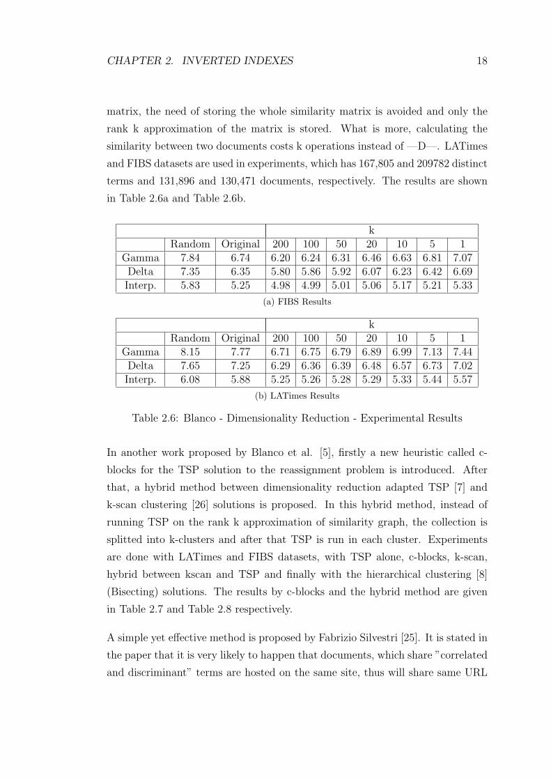
and FIBS datasets are used in experiments, which has 167,805 and 209782 distinct
terms and 131,896 and 130,471 documents, respectively. The results are shown
in Table 2.6a and Table 2.6b.
kRandom Original 200 100 50 20 10 5 1
Gamma 7.84 6.74 6.20 6.24 6.31 6.46 6.63 6.81 7.07Delta 7.35 6.35 5.80 5.86 5.92 6.07 6.23 6.42 6.69Interp. 5.83 5.25 4.98 4.99 5.01 5.06 5.17 5.21 5.33
(a) FIBS Results
kRandom Original 200 100 50 20 10 5 1
Gamma 8.15 7.77 6.71 6.75 6.79 6.89 6.99 7.13 7.44Delta 7.65 7.25 6.29 6.36 6.39 6.48 6.57 6.73 7.02Interp. 6.08 5.88 5.25 5.26 5.28 5.29 5.33 5.44 5.57
(b) LATimes Results
Table 2.6: Blanco - Dimensionality Reduction - Experimental Results
In another work proposed by Blanco et al. [5], firstly a new heuristic called c-
blocks for the TSP solution to the reassignment problem is introduced. After
that, a hybrid method between dimensionality reduction adapted TSP [7] and
k-scan clustering [26] solutions is proposed. In this hybrid method, instead of
running TSP on the rank k approximation of similarity graph, the collection is
splitted into k-clusters and after that TSP is run in each cluster. Experiments
are done with LATimes and FIBS datasets, with TSP alone, c-blocks, k-scan,
hybrid between kscan and TSP and finally with the hierarchical clustering [8]
(Bisecting) solutions. The results by c-blocks and the hybrid method are given
in Table 2.7 and Table 2.8 respectively.
A simple yet effective method is proposed by Fabrizio Silvestri [25]. It is stated in
the paper that it is very likely to happen that documents, which share ”correlated
and discriminant” terms are hosted on the same site, thus will share same URL
CHAPTER 2. INVERTED INDEXES 19
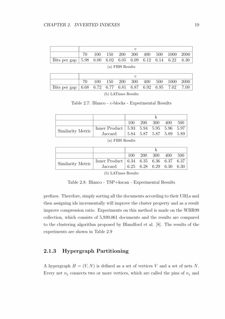
c70 100 150 200 300 400 500 1000 2000
Bits per gap 5.98 6.00 6.02 6.05 6.09 6.12 6.14 6.22 6.30
(a) FIBS Results
c70 100 150 200 300 400 500 1000 2000
Bits per gap 6.68 6.72 6.77 6.81 6.87 6.92 6.95 7.02 7.09
(b) LATimes Results
Table 2.7: Blanco - c-blocks - Experimental Results
k100 200 300 400 500
Similarity MetricInner Product 5.93 5.94 5.95 5.96 5.97
Jaccard 5.84 5.87 5.87 5.89 5.89
(a) FIBS Results
k100 200 300 400 500
Similarity MetricInner Product 6.34 6.35 6.36 6.37 6.37
Jaccard 6.25 6.28 6.29 6.30 6.30
(b) LATimes Results
Table 2.8: Blanco - TSP+kscan - Experimental Results
prefixes. Therefore, simply sorting all the documents according to their URLs and
then assigning ids incrementally will improve the cluster property and as a result
improve compression ratio. Experiments on this method is made on the WBR99
collection, which consists of 5,939,061 documents and the results are compared
to the clustering algorithm proposed by Blandford et al. [8]. The results of the
experiments are shown in Table 2.9
2.1.3 Hypergraph Partitioning
A hypergraph H = (V,N) is defined as a set of vertices V and a set of nets N .
Every net nj connects two or more vertices, which are called the pins of nj and
CHAPTER 2. INVERTED INDEXES 20
VB Gamma Delta S9 Interp. GolombRandom 11.4 12.72 12.71 15.41 11.13 11.31Original 11.25 12.34 12.32 15.2 10.94 11.12
Url sorting 9.72 7.72 7.69 14.34 7.48 8.23Clustering 9.81 8.82 8.8 14.03 7.26 8.63
Clustering+Url sorting 10.03 8.96 8.95 14.15 7.31 8.9
Table 2.9: Silvestri Sorting Out Work Experimental Results
denoted by pins[nj] and inversely, the subset of nets, which connect a vertex vi to
other vertices are called the nets of vi and denoted by nets[vi]. Graph is a subset
of hypergraph, where each net connects exactly two vertices. Every vertex vi has
a weight denoted by wi and every net nj has a cost denoted by cj. A K-way
partitioning of a hypergraph H is defined as Π = {V1, V2, ..., VK}, where ∀i, j,
1 ≤ i, j ≤ K and i 6= j, Vi 6= ∅, Vi ∩ Vj = ∅ and⋃
Vi = V . In a partition Π, nj is
said to connect a part if it has at least one pin which belongs to that part. The
set of parts which nj connects is called the connectivity set of nj and denoted
by Λj. The cardinality of Λj, which is the number of parts that nj connects is
denoted by λj. A net nj is said to be an internal net if λj = 1 and external net
if λj > 1. The internal and external nets are also referred as uncut and cut nets,
respectively. The weight of a part Vi is the sum of weights of vertices belonging
to Vi and is denoted by Wi. A partitioning Π is said to be balanced if it satisfies
the balance criterion:
Wk ≤ Wavg(1 + ε), fork = 1, 2, ..., K (2.1)
The cost of a partitioning X(Π), which is also referred as cutsize of the partition-
ing, has various definitions. Two most common definitions are:
X(Π) =∑
nj∈NE
cj (2.2a)
X(Π) =∑
nj∈NE
cj(λj − 1) (2.2b)
where NE denotes the set of external nets. As a result, hypergraph partitioning
problem is defined as dividing a hypergraph into two or more parts while mini-
mizing the cutsize and satisfying the balance criterion 2.1 among the part weights
[3].
CHAPTER 2. INVERTED INDEXES 21
2.1.3.1 Related Works based on Hypergraph Partitioning
Hypergraph partitioning models have gained great attention because it can be
adapted to many problems. A very famous example is the sparse-matrix par-
titioning problem. Many problems in parallel computing have been reduced to
the partitioning of sparse-matrices and solved by adapting hypergraph partition-
ing based models [3, 23, 10, 30, 29]. Hypergraph partitioning models are also
adapted to task scheduling in master-slave environments [17], data-pattern-based
clustering [16, 22] and direct volume rendering problems [9].
Chapter 3
Inverted Index Compression
Based on Term and Document
Identifier Reassignment
As stated in Aykanat et al.’s paper [4], block-diagonal structure of sparse matrices
has been exploited for parallelization of various algorithms such as decomposition
methods for linear programming, LU factorization and QR factorization. In Fig-
ure 3.1, a K-way singly bordered block-diagonal form, also referred to as SB form,
of an M × N sparse matrix is illustrated, which consists of K + 1 submatrices
including the border R = (R1R2...RK). Each row in the border has nonzeros in
the columns of at least two of K diagonal blocks.
The transformation of a matrix into its block-diagonal form is a recent problem.
Ferris et al. [14] proposed a two-phase approach for this problem, where in the
first phase the matrix is transformed into an intermediate form and then in the
second phase the intermediate form of the matrix is transformed into a block-
diagonal form. Aykanat et al. [4] proposed two models. In one model, the sparse
matrix is represented as a graph and the transformation problem is reduced to
the graph partitioning by vertex seperator (GPVS) problem whereas in the other
model the matrix is represented as a hypergraph and the transformation problem
22
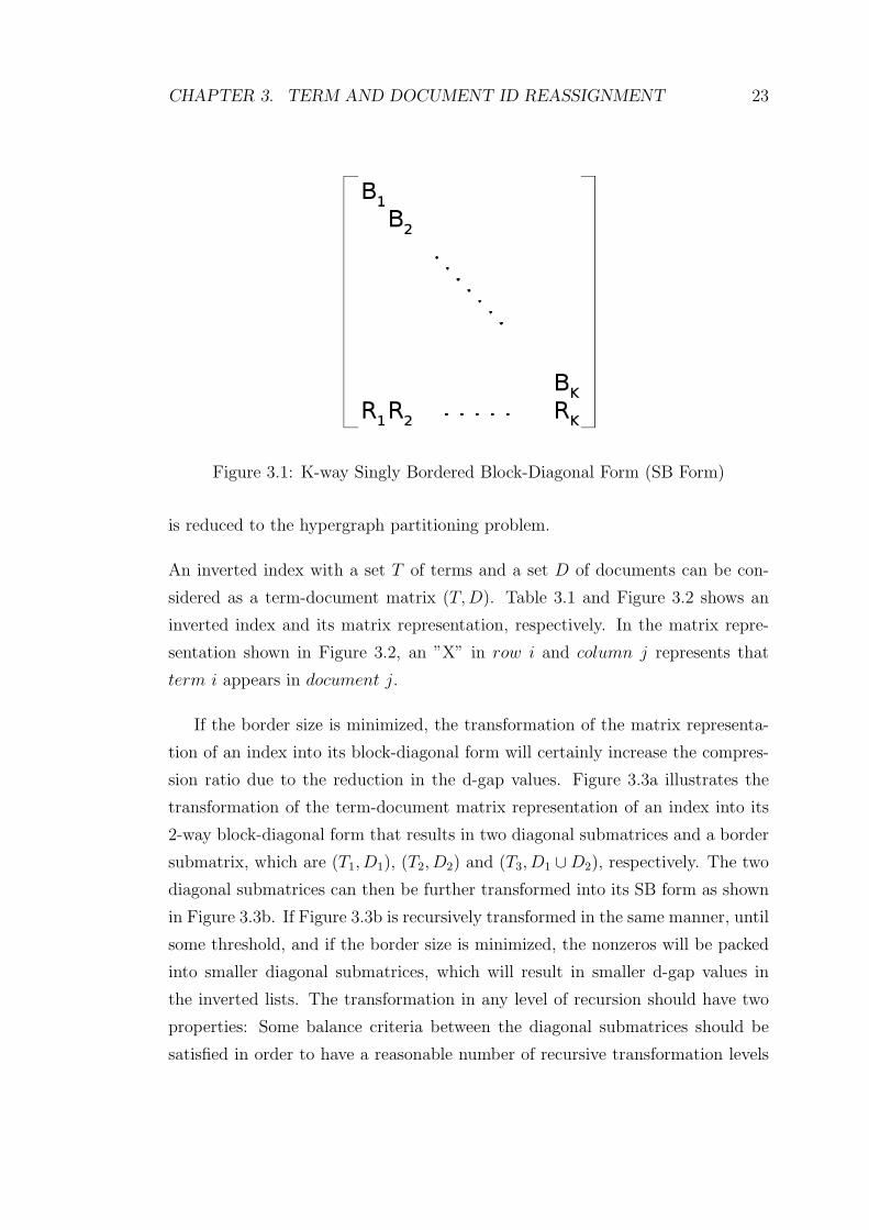
CHAPTER 3. TERM AND DOCUMENT ID REASSIGNMENT 23
Figure 3.1: K-way Singly Bordered Block-Diagonal Form (SB Form)
is reduced to the hypergraph partitioning problem.
An inverted index with a set T of terms and a set D of documents can be con-
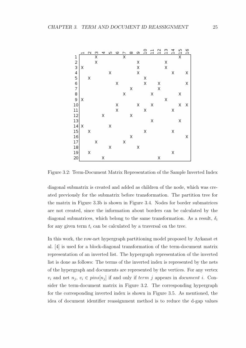
sidered as a term-document matrix (T,D). Table 3.1 and Figure 3.2 shows an
inverted index and its matrix representation, respectively. In the matrix repre-
sentation shown in Figure 3.2, an ”X” in row i and column j represents that
term i appears in document j.
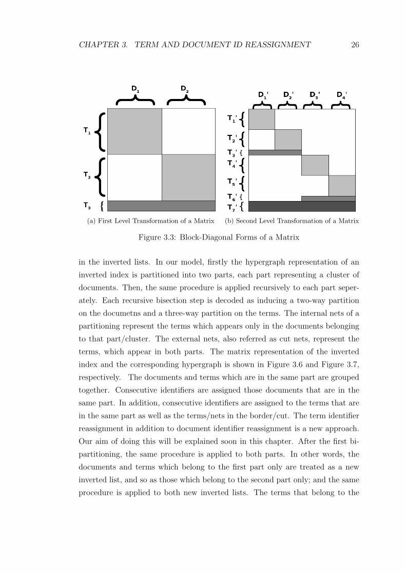
If the border size is minimized, the transformation of the matrix representa-
tion of an index into its block-diagonal form will certainly increase the compres-
sion ratio due to the reduction in the d-gap values. Figure 3.3a illustrates the
transformation of the term-document matrix representation of an index into its
2-way block-diagonal form that results in two diagonal submatrices and a border
submatrix, which are (T1, D1), (T2, D2) and (T3, D1 ∪ D2), respectively. The two
diagonal submatrices can then be further transformed into its SB form as shown
in Figure 3.3b. If Figure 3.3b is recursively transformed in the same manner, until
some threshold, and if the border size is minimized, the nonzeros will be packed
into smaller diagonal submatrices, which will result in smaller d-gap values in
the inverted lists. The transformation in any level of recursion should have two
properties: Some balance criteria between the diagonal submatrices should be
satisfied in order to have a reasonable number of recursive transformation levels
CHAPTER 3. TERM AND DOCUMENT ID REASSIGNMENT 24
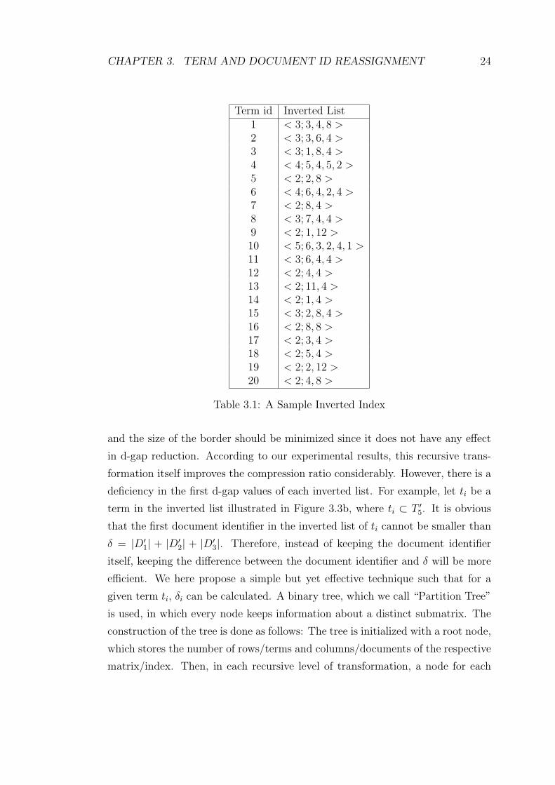
Term id Inverted List1 < 3; 3, 4, 8 >2 < 3; 3, 6, 4 >3 < 3; 1, 8, 4 >4 < 4; 5, 4, 5, 2 >5 < 2; 2, 8 >6 < 4; 6, 4, 2, 4 >7 < 2; 8, 4 >8 < 3; 7, 4, 4 >9 < 2; 1, 12 >10 < 5; 6, 3, 2, 4, 1 >11 < 3; 6, 4, 4 >12 < 2; 4, 4 >13 < 2; 11, 4 >14 < 2; 1, 4 >15 < 3; 2, 8, 4 >16 < 2; 8, 8 >17 < 2; 3, 4 >18 < 2; 5, 4 >19 < 2; 2, 12 >20 < 2; 4, 8 >
Table 3.1: A Sample Inverted Index
and the size of the border should be minimized since it does not have any effect
in d-gap reduction. According to our experimental results, this recursive trans-
formation itself improves the compression ratio considerably. However, there is a
deficiency in the first d-gap values of each inverted list. For example, let ti be a
term in the inverted list illustrated in Figure 3.3b, where ti ⊂ T ′5. It is obvious
that the first document identifier in the inverted list of ti cannot be smaller than
δ = |D′1| + |D′
2| + |D′3|. Therefore, instead of keeping the document identifier
itself, keeping the difference between the document identifier and δ will be more
efficient. We here propose a simple but yet effective technique such that for a
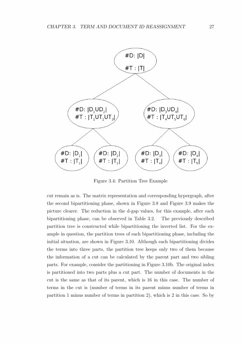
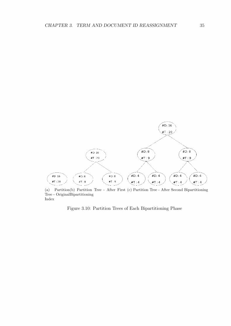
given term ti, δi can be calculated. A binary tree, which we call “Partition Tree”
is used, in which every node keeps information about a distinct submatrix. The
construction of the tree is done as follows: The tree is initialized with a root node,
which stores the number of rows/terms and columns/documents of the respective
matrix/index. Then, in each recursive level of transformation, a node for each
CHAPTER 3. TERM AND DOCUMENT ID REASSIGNMENT 25
Figure 3.2: Term-Document Matrix Representation of the Sample Inverted Index
diagonal submatrix is created and added as children of the node, which was cre-
ated previously for the submatrix before transformation. The partition tree for
the matrix in Figure 3.3b is shown in Figure 3.4. Nodes for border submatrices
are not created, since the information about borders can be calculated by the
diagonal submatrices, which belong to the same transformation. As a result, δi
for any given term ti can be calculated by a traversal on the tree.
In this work, the row-net hypergraph partitioning model proposed by Aykanat et
al. [4] is used for a block-diagonal transformation of the term-document matrix
representation of an inverted list. The hypergraph representation of the inverted
list is done as follows: The terms of the inverted index is represented by the nets
of the hypergraph and documents are represented by the vertices. For any vertex
vi and net nj, vi ∈ pins[nj] if and only if term j appears in document i. Con-
sider the term-document matrix in Figure 3.2. The corresponding hypergraph
for the corresponding inverted index is shown in Figure 3.5. As mentioned, the
idea of document identifier reassignment method is to reduce the d-gap values
CHAPTER 3. TERM AND DOCUMENT ID REASSIGNMENT 26
(a) First Level Transformation of a Matrix (b) Second Level Transformation of a Matrix
Figure 3.3: Block-Diagonal Forms of a Matrix
in the inverted lists. In our model, firstly the hypergraph representation of an
inverted index is partitioned into two parts, each part representing a cluster of
documents. Then, the same procedure is applied recursively to each part seper-
ately. Each recursive bisection step is decoded as inducing a two-way partition
on the documetns and a three-way partition on the terms. The internal nets of a
partitioning represent the terms which appears only in the documents belonging
to that part/cluster. The external nets, also referred as cut nets, represent the
terms, which appear in both parts. The matrix representation of the inverted
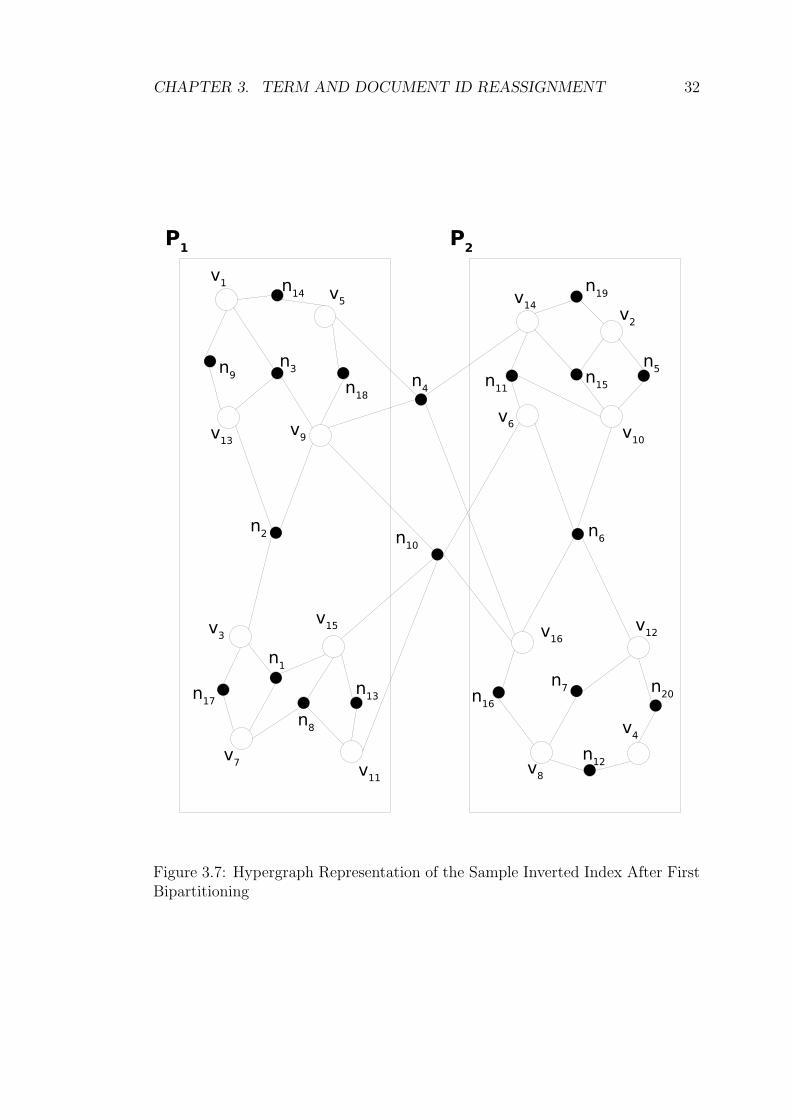
index and the corresponding hypergraph is shown in Figure 3.6 and Figure 3.7,
respectively. The documents and terms which are in the same part are grouped
together. Consecutive identifiers are assigned those documents that are in the
same part. In addition, consecutive identifiers are assigned to the terms that are
in the same part as well as the terms/nets in the border/cut. The term identifier
reassignment in addition to document identifier reassignment is a new approach.
Our aim of doing this will be explained soon in this chapter. After the first bi-
partitioning, the same procedure is applied to both parts. In other words, the
documents and terms which belong to the first part only are treated as a new
inverted list, and so as those which belong to the second part only; and the same
procedure is applied to both new inverted lists. The terms that belong to the
CHAPTER 3. TERM AND DOCUMENT ID REASSIGNMENT 27
Figure 3.4: Partition Tree Example
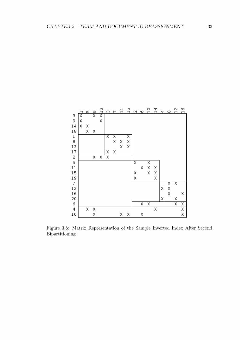
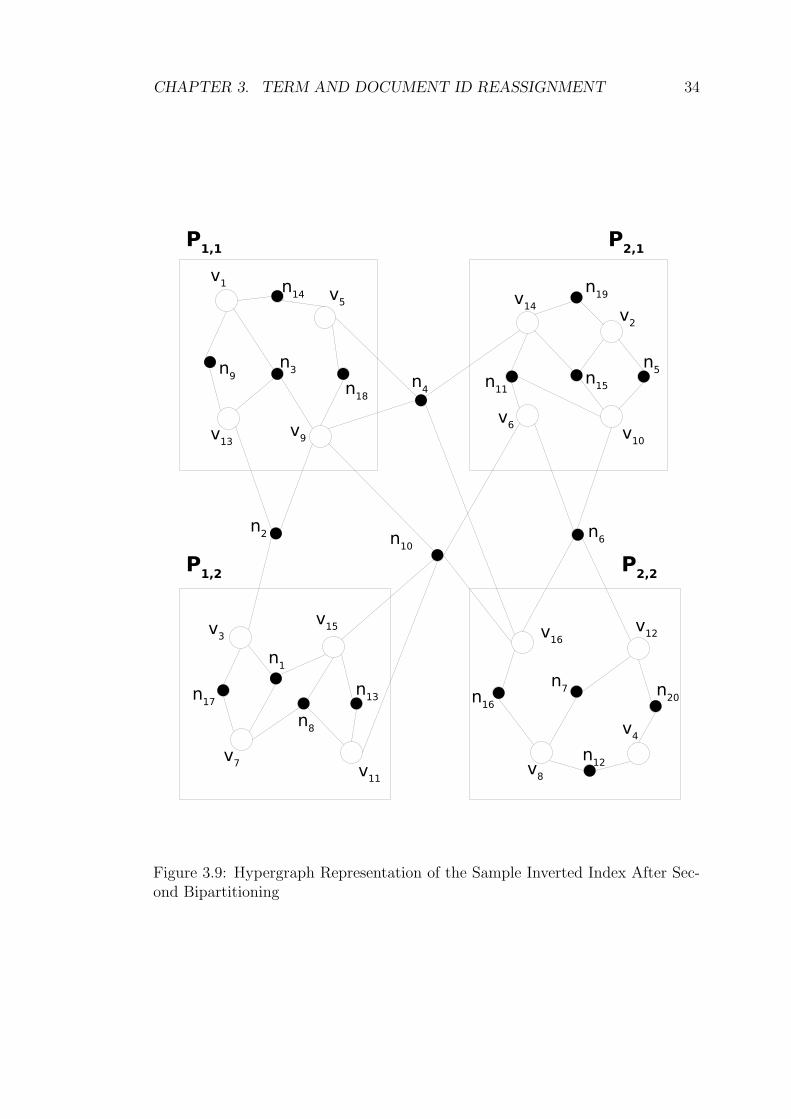
cut remain as is. The matrix representation and corresponding hypergraph, after
the second bipartitioning phase, shown in Figure 3.8 and Figure 3.9 makes the
picture clearer. The reduction in the d-gap values, for this example, after each
bipartitioning phase, can be observed in Table 3.2. The previously described
partition tree is constructed while bipartitioning the inverted list. For the ex-
ample in question, the partition trees of each bipartitioning phase, including the
initial situation, are shown in Figure 3.10. Although each bipartitioning divides
the terms into three parts, the partition tree keeps only two of them because
the information of a cut can be calculated by the parent part and two sibling
parts. For example, consider the partitioning in Figure 3.10b. The original index
is partitioned into two parts plus a cut part. The number of documents in the
cut is the same as that of its parent, which is 16 in this case. The number of
terms in the cut is (number of terms in its parent minus number of terms in
partition 1 minus number of terms in partition 2), which is 2 in this case. So by
CHAPTER 3. TERM AND DOCUMENT ID REASSIGNMENT 28
Term id Init.Termid
Inverted List
1 1 < 3; 2, 2, 4 >2 2 < 3; 2, 3, 2 >3 3 < 3; 1, 4, 2 >4 8 < 3; 4, 2, 2 >5 9 < 2; 1, 6 >6 13 < 2; 6, 2 >7 14 < 2; 1, 2 >8 17 < 2; 2, 2 >9 18 < 2; 3, 2 >10 5 < 2; 9, 4 >11 6 < 4; 11, 2, 1, 2 >12 7 < 2; 12, 2 >13 11 < 3; 11, 2, 2 >14 12 < 2; 10, 2 >15 15 < 3; 9, 4, 2 >16 16 < 2; 12, 4 >17 19 < 2; 9, 6 >18 20 < 2; 10, 4 >19 4 < 4; 3, 2, 10, 1 >20 10 < 5; 5, 1, 2, 3, 5 >
(a) D-gaps after first bipartitioning of Indexin Table 3.1
Term id Init.Termid
Inverted List
1 3 < 3; 1, 2, 1 >2 9 < 2; 1, 3 >3 14 < 2; 1, 1 >4 18 < 2; 2, 1 >5 1 < 3; 5, 1, 2 >6 8 < 3; 6, 1, 1 >7 13 < 2; 7, 1 >8 17 < 2; 5, 1 >9 2 < 3; 3, 1, 1 >10 5 < 2; 9, 2 >11 11 < 3; 10, 1, 1 >12 15 < 3; 9, 2, 1 >13 19 < 2; 9, 3 >14 7 < 2; 14, 1 >15 12 < 2; 13, 1 >16 16 < 2; 14, 2 >17 20 < 2; 13, 2 >18 6 < 4; 10, 1, 4, 1 >19 4 < 4; 2, 1, 9, 4 >20 10 < 5; 3, 4, 1, 2, 6 >
(b) D-gaps after second bipartitioning of Indexin Table 3.1
Table 3.2: The d-gap representations of inverted lists in each bipartitioning phase
this partition tree, given a reassigned term id, the part that it belongs to and the
minimum document identifier that can be in the inverted list of this term can
be calculated by a traversal on this tree and consequently, the first d-gap value
can be replaced by the difference between the first document identifier and the
minimum document identifier. According to this improvement, the final inverted
lists of each bipartitioning phase is shown in Table 3.3.
CHAPTER 3. TERM AND DOCUMENT ID REASSIGNMENT 29
Term id Init.Termid
Inverted List
1 1 < 3; 2, 2, 4 >2 2 < 3; 2, 3, 2 >3 3 < 3; 1, 4, 2 >4 8 < 3; 4, 2, 2 >5 9 < 2; 1, 6 >6 13 < 2; 6, 2 >7 14 < 2; 1, 2 >8 17 < 2; 2, 2 >9 18 < 2; 3, 2 >10 5 < 2; 1, 4 >11 6 < 4; 3, 2, 1, 2 >12 7 < 2; 4, 2 >13 11 < 3; 3, 2, 2 >14 12 < 2; 2, 2 >15 15 < 3; 1, 4, 2 >16 16 < 2; 4, 4 >17 19 < 2; 1, 6 >18 20 < 2; 2, 4 >19 4 < 4; 3, 2, 10, 1 >20 10 < 5; 5, 1, 2, 3, 5 >
(a) D-gaps after first bipartitioning using Par-tition Tree
Term id Init.Termid
Inverted List
1 3 < 3; 1, 2, 1 >2 9 < 2; 1, 3 >3 14 < 2; 1, 1 >4 18 < 2; 2, 1 >5 1 < 3; 1, 1, 2 >6 8 < 3; 2, 1, 1 >7 13 < 2; 3, 1 >8 17 < 2; 1, 1 >9 2 < 3; 3, 1, 1 >10 5 < 2; 1, 2 >11 11 < 3; 2, 1, 1 >12 15 < 3; 1, 2, 1 >13 19 < 2; 1, 3 >14 7 < 2; 2, 1 >15 12 < 2; 1, 1 >16 16 < 2; 2, 2 >17 20 < 2; 1, 2 >18 6 < 4; 2, 1, 4, 1 >19 4 < 4; 2, 1, 9, 4 >20 10 < 5; 3, 4, 1, 2, 6 >
(b) D-gaps after second bipartitioning usingPartition Tree
Table 3.3: d-gap representations of inverted lists in each bipartitioning phaseusing Partition Tree
CHAPTER 3. TERM AND DOCUMENT ID REASSIGNMENT 30
Figure 3.5: Hypergraph Representation of the Sample Inverted Index
CHAPTER 3. TERM AND DOCUMENT ID REASSIGNMENT 31
Figure 3.6: Matrix Representation of the Sample Inverted Index After First Bi-partitioning
CHAPTER 3. TERM AND DOCUMENT ID REASSIGNMENT 32
Figure 3.7: Hypergraph Representation of the Sample Inverted Index After FirstBipartitioning
CHAPTER 3. TERM AND DOCUMENT ID REASSIGNMENT 33
Figure 3.8: Matrix Representation of the Sample Inverted Index After SecondBipartitioning
CHAPTER 3. TERM AND DOCUMENT ID REASSIGNMENT 34
Figure 3.9: Hypergraph Representation of the Sample Inverted Index After Sec-ond Bipartitioning
CHAPTER 3. TERM AND DOCUMENT ID REASSIGNMENT 35
(a) PartitionTree - OriginalIndex
(b) Partition Tree - After FirstBipartitioning
(c) Partition Tree - After Second Bipartitioning
Figure 3.10: Partition Trees of Each Bipartitioning Phase
Chapter 4
Implementation & Experimental
Results
To assess the performance of our technique, we tested it on two different collec-
tions. One of them is an extended version of the Google Programming Contest
Collection1, which will be referred as google-plus and the other one is a rather
smaller collection, which is crawled from the site of a newspaper called Radikal
and will be referred as radikal. Google-plus consists of 1,567,240 documents,
3,275,075 terms and 22,223,170 appearances of terms whereas radikal consists
of 6,887 documents, 109,558 terms and 252,752 appearances of terms.
We implemented four independent modules to test the performance of our algo-
rithm. The Doc-Term-Id-Reassigner Module takes the inverted index as input and
outputs reassignment of document and term identifiers as well as the Partition
Tree, which is discussed previously. A Hypergraph Partitioning Tool, PaToH[3],
is used by this module for the hypergraph partitioning based transformation into
SB-form. Index-Rebuilder Module takes the original inverted index as well as
the document and term id remappings as input, and outputs the remapped in-
verted index. Compression-Ratio-Evaluator module takes an inverted index as
1http://www.google.com/programming-contest
36
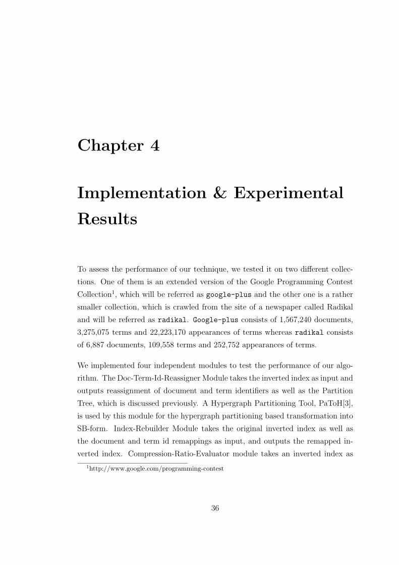
CHAPTER 4. IMPLEMENTATION & EXPERIMENTAL RESULTS 37
input, and outputs the number of bits required to compress it without consid-
ering the Partition-Tree. It is used to evaluate the compression ratio of both
original and remapped indexes individually. Partition-Tree-Aware-Compression-
Ratio-Evaluator takes the remapped inverted index as well as the partition tree
as input, and outputs the number of bits required to compress it by considering
the improvement achieved by the partition-tree. The flow of an experiment and
the interrelations between modules are illustrated in Figure 4.1.
Figure 4.1: Interrelations of Modules used in Experimental Analysis
CHAPTER 4. IMPLEMENTATION & EXPERIMENTAL RESULTS 38
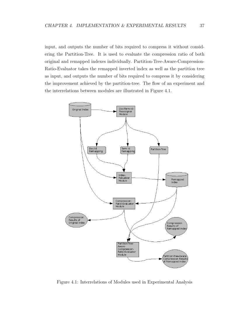
We used three different compression schemes to evaluate the improvement in
the compression of the inverted files: gamma coding, delta coding and huffman
coding. In addition, we constructed a randomized version of each collection (ran-
domly assigned document and term identifiers) to observe the efficiency of our
algorithm more effectively. Table 4.1 and Table 4.2 show the compression results
on original and randomized radikal collections, respectively. Both the size of the
compressed index and the percent of improvements are presented in the results.
In addition, in order to see the effect of the partition tree, the results with and
without using partition tree are taken seperately. The significant increase can be
observed in all compression schemes.
Compression Schemegamma delta huffman
Size(Mbits)
Improv. Size(Mbits)
Improv. Size(Mbits)
Improv.
Original 4.91 0 4.02 0 3.04 0Reassigned 4.67 4.85% 3.87 3.88% 2.96 2.52%Reassigned(Partition TreeAware)
3.44 29.93% 3.03 24.70% 2.45 29.32%
Table 4.1: Results on Original Radikal Collection
Compression Schemegamma delta huffman
Size(Mbits)
Improv. Size(Mbits)
Improv. Size(Mbits)
Improv.
Randomized 5.04 0 4.12 0 3.05 0Reassigned 4.77 5.22% 3.92 4.90% 3.00 1.78%Reassigned(Partition TreeAware)
3.43 31.87% 3.01 26.91% 2.45 19.56%
Table 4.2: Results on Randomized Radikal Collection
As mentioned, our algorithm recursively creates singly bordered block-diagonal
forms of the sparse-matrix representation of an inverted list. Therefore, it is ex-
pected to happen that the compression ratio increases as the maximum level of
CHAPTER 4. IMPLEMENTATION & EXPERIMENTAL RESULTS 39
recursion increases. This is not always the case as we observed from the exper-
iments. Very rarely, the compression ratio decreases while the level of recursion
increases. However, these reductions are too small to consider, so we can safely
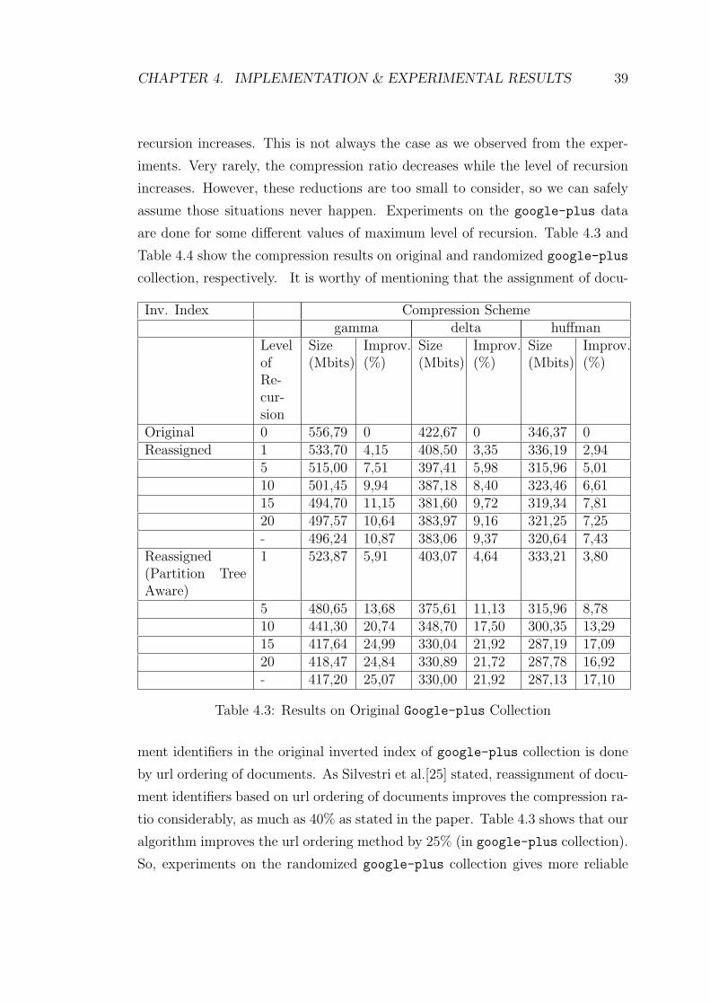
assume those situations never happen. Experiments on the google-plus data
are done for some different values of maximum level of recursion. Table 4.3 and
Table 4.4 show the compression results on original and randomized google-plus
collection, respectively. It is worthy of mentioning that the assignment of docu-
Inv. Index Compression Schemegamma delta huffman
LevelofRe-cur-sion
Size(Mbits)
Improv.(%)
Size(Mbits)
Improv.(%)
Size(Mbits)
Improv.(%)
Original 0 556,79 0 422,67 0 346,37 0Reassigned 1 533,70 4,15 408,50 3,35 336,19 2,94
5 515,00 7,51 397,41 5,98 315,96 5,0110 501,45 9,94 387,18 8,40 323,46 6,6115 494,70 11,15 381,60 9,72 319,34 7,8120 497,57 10,64 383,97 9,16 321,25 7,25- 496,24 10,87 383,06 9,37 320,64 7,43
Reassigned(Partition TreeAware)
1 523,87 5,91 403,07 4,64 333,21 3,80
5 480,65 13,68 375,61 11,13 315,96 8,7810 441,30 20,74 348,70 17,50 300,35 13,2915 417,64 24,99 330,04 21,92 287,19 17,0920 418,47 24,84 330,89 21,72 287,78 16,92- 417,20 25,07 330,00 21,92 287,13 17,10
Table 4.3: Results on Original Google-plus Collection
ment identifiers in the original inverted index of google-plus collection is done
by url ordering of documents. As Silvestri et al.[25] stated, reassignment of docu-
ment identifiers based on url ordering of documents improves the compression ra-
tio considerably, as much as 40% as stated in the paper. Table 4.3 shows that our
algorithm improves the url ordering method by 25% (in google-plus collection).
So, experiments on the randomized google-plus collection gives more reliable
CHAPTER 4. IMPLEMENTATION & EXPERIMENTAL RESULTS 40
Inv. Index Compression Schemegamma delta huffman
LevelofRe-cur-sion
Size(Mbits)
Improv.(%)
Size(Mbits)
Improv.(%)
Size(Mbits)
Improv.(%)
Original 0 648,25 0 487,18 0 381,54 0Reassigned 1 615,06 5,12 466,48 4,25 366,61 3,91
5 579,19 10,65 444,66 8,73 354,19 7,1710 546,63 15,68 421,97 13,38 343,86 9,8715 530,37 18,18 408,37 16,18 336,29 11,8520 527,64 18,61 406,54 16,55 335,04 12,19- 527,78 18,58 406,66 16,53 335,15 12,16
Reassigned(Partition TreeAware)
1 603,07 6,97 459,55 5,67 362,57 4,97
5 543,80 16,11 422,26 13,32 340,13 10,8510 485,75 25,07 382,94 21,39 320,22 16,0715 450,56 30,50 355,11 27,11 303,81 20,3720 448,42 30,83 353,36 27,47 301,99 20,85- 448,60 30,80 353,55 27,43 302,16 20,81
Table 4.4: Results on Randomized Google-plus Collection
results. Furthermore, if the url ordering method and our method is combined,
what we mean is given an inverted list, first url ordering method and then our
SB-form-based method are applied, the results gets better, as shown in Table 4.5,
which is obtained by combining Table 4.3 and Table 4.4. The maximum improve-
ment in compression ratio is about 35,5% by gamma coding, which is reached at
the 15th level of recursion. This is the best result to the best of our knowledge.
Silvestri[25] achieved 40% in WBR99 collection. However, if the additional 25%
improvement of our algorithm on url ordering method on Google-plus data is
considered, the improvement of our algorithm may very probably exceed 50% on
WBR99 collection.
The delta coding performs 32,2% improvement, almost as much as gamma coding.
However, it is 20% better than gamma coding in terms of the compressed index
size, which is almost as small as the size with huffman coding. It is known
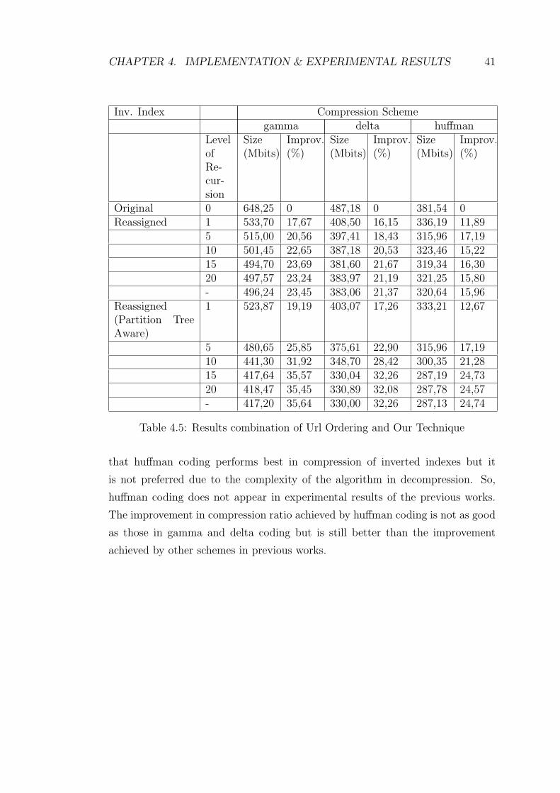
CHAPTER 4. IMPLEMENTATION & EXPERIMENTAL RESULTS 41
Inv. Index Compression Schemegamma delta huffman
LevelofRe-cur-sion
Size(Mbits)
Improv.(%)
Size(Mbits)
Improv.(%)
Size(Mbits)
Improv.(%)
Original 0 648,25 0 487,18 0 381,54 0Reassigned 1 533,70 17,67 408,50 16,15 336,19 11,89
5 515,00 20,56 397,41 18,43 315,96 17,1910 501,45 22,65 387,18 20,53 323,46 15,2215 494,70 23,69 381,60 21,67 319,34 16,3020 497,57 23,24 383,97 21,19 321,25 15,80- 496,24 23,45 383,06 21,37 320,64 15,96
Reassigned(Partition TreeAware)
1 523,87 19,19 403,07 17,26 333,21 12,67
5 480,65 25,85 375,61 22,90 315,96 17,1910 441,30 31,92 348,70 28,42 300,35 21,2815 417,64 35,57 330,04 32,26 287,19 24,7320 418,47 35,45 330,89 32,08 287,78 24,57- 417,20 35,64 330,00 32,26 287,13 24,74
Table 4.5: Results combination of Url Ordering and Our Technique
that huffman coding performs best in compression of inverted indexes but it
is not preferred due to the complexity of the algorithm in decompression. So,
huffman coding does not appear in experimental results of the previous works.
The improvement in compression ratio achieved by huffman coding is not as good
as those in gamma and delta coding but is still better than the improvement
achieved by other schemes in previous works.
Chapter 5
Conclusion & Future Work
As it is clearly shown, reassigning document identifiers of an inverted index by
transforming the term-document matrix representation of the index into its singly
bordered block-diagonal form efficiently reduces the d-gap values. The experimen-
tal results of the previous works are also presented in order to make a comparison.
It is observed that the presented work performs best up until now in terms of
compression ratio.
A novel data structure, which is called Partition-Tree, is also proposed. Ex-
perimental results, with and without using it are presented seperately in order
to show its effect. With the help of Partition-Tree, any information specific to
a cluster can be stored and retrieved efficiently. For future work, different com-
pression schemes can be applied to each cluster and the scheme that is specific
to a cluster can be stored in the tree.
In this work, term identifier reassignment is also applied, in addition to doc-
ument identifier reassignment. This is a new approach and it makes it easy to
keep common properties of the posting lists of the terms that are in the same
cluster. Then, these properties can be used for more efficient compression, which
is the case observed in our work.
42
Bibliography
[1] V. N. Anh and A. Moffat. Index compression using fixed binary codewords.
In ADC ’04: Proceedings of the 15th Australasian database conference, pages
61–67, Darlinghurst, Australia, Australia, 2004. Australian Computer Soci-
ety, Inc.
[2] V. N. Anh and A. Moffat. Inverted index compression using word-aligned
binary codes. Inf. Retr., 8(1):151–166, 2005.
[3] U. V. C. Atalyurek and C. Aykanat. Hypergraph-partitioning based decom-
position for parallel sparse-matrix vector multiplication. IEEE Trans. on
Parallel and Distributed Computing, 10:673–693, 1999.
[4] C. Aykanat and A. Pinar. Permuting sparse rectangular matrices into block-
diagonal form. SIAM J. Scientific Computing, 25:1860–1879.
[5] R. Blanco and Alvaro Barreiro. Tsp and cluster-based solutions to the reas-
signment of document identifiers. Inf. Retr., 9(4):499–517, 2006.
[6] R. Blanco and A. Barreiro. Characterization of a simple case of the reas-
signment of document identifiers as a pattern sequencing problem. In SIGIR
’05: Proceedings of the 28th annual international ACM SIGIR conference
on Research and development in information retrieval, pages 587–588, New
York, NY, USA, 2005. ACM.
[7] R. Blanco and A. Barreiro. Document identier reassignment through di-
mensionality reduction. In Proceedings of the 27th European Conference on
Information Retrieval, pages 375–387, 2005.
43
BIBLIOGRAPHY 44
[8] D. Blandford and G. Blelloch. Index compression through document reorder-
ing. In DCC ’02: Proceedings of the Data Compression Conference (DCC
’02), page 342, Washington, DC, USA, 2002. IEEE Computer Society.
[9] B. B. Cambazoglu. Hypergraph-partitioning-based remapping models for
image-space-parallel direct volume rendering of unstructured grids. IEEE
Trans. Parallel Distrib. Syst., 18(1):3–16, 2007. Member-Cevdet Aykanat.
[10] U. Catalyurek and C. Aykanat. Decomposing irregularly sparse matrices
for parallel matrix-vector multiplication. In IRREGULAR ’96: Proceedings
of the Third International Workshop on Parallel Algorithms for Irregularly
Structured Problems, pages 75–86, London, UK, 1996. Springer-Verlag.
[11] J. Chen and T. Cook. Using d-gap patterns for index compression. In WWW
’07: Proceedings of the 16th international conference on World Wide Web,
pages 1209–1210, New York, NY, USA, 2007. ACM.
[12] J. Chen, P. Zhong, and T. Cook. Improving index compression using cluster
information. In WI ’06: Proceedings of the 2006 IEEE/WIC/ACM Inter-
national Conference on Web Intelligence, pages 188–194, Washington, DC,
USA, 2006. IEEE Computer Society.
[13] P. Elias. Universal codeword sets and representations of the integers. IEEE
Transactions on Information Theory, (21), 1975.
[14] M. C. Ferris and J. D. Horn. Partitioning mathematical programs for parallel
solution. Technical report, Mathematical Programming, 1994.
[15] A. Gelbukh, S. Han, and G. Sidorov. Compression of boolean inverted files by
document ordering. In Proceedings of 2003 IEEE international conference
on natural language processing and knowledge engineering, pages 244–249.
IEEE Computer Society Press, 2003.
[16] E. H. Han, G. Karypis, V. Kumar, and B. Mobasher. Clustering in a high
dimensional space using hypergraph models. Technical report, University of
Minnesota, Department of Computer Science, 1997.
BIBLIOGRAPHY 45
[17] K. Kaya. Iterative-improvement-based heuristics for adaptive scheduling of
tasks sharing files on heterogeneous master-slave environments. IEEE Trans.
Parallel Distrib. Syst., 17(8):883–896, 2006. Member-Cevdet Aykanat.
[18] C.-H. Lai and T.-F. Chen. Compressing inverted files in scalable information
systems by binary decision diagram encoding. In Supercomputing ’01: Pro-
ceedings of the 2001 ACM/IEEE conference on Supercomputing (CDROM),
pages 60–60, New York, NY, USA, 2001. ACM.
[19] A. Moffat and J. S. Culpepper. Hybrid bitvector index compression. In Proc.
12th Australasian Document Computing Symposium (ADCS), pages 25–31,
2007.
[20] A. Moffat and L. Stuiver. Binary interpolative coding for effective index
compression. Inf. Retr., 3(1):25–47, 2000.
[21] I. Nitsos, G. Evangelidis, and D. Dervos. g-binary: A new non-parameterized
code for improved inverted file compression. In V. Mark, W. Retschitzegger,
and O. Stepnkov, editors, DEXA, volume 2736 of Lecture Notes in Computer
Science, pages 464–473. Springer, 2003.
[22] M. M. Ozdal and C. Aykanat. Hypergraph models and algorithms for dat-
apattern based clustering. Data Mining and Knowledge Discovery, 9:29–57,
2004.
[23] A. Pinar, U. V. C. Atalyurek, C. Aykanat, and M. Pinar. Decomposing
linear programs for parallel solution. In Lecture Notes in Computer Science,
pages 473–482. Springer-Verlag, 1996.
[24] W.-Y. Shieh, T.-F. Chen, J. J.-J. Shann, and C.-P. Chung. Inverted file com-
pression through document identifier reassignment. Inf. Process. Manage.,
39(1):117–131, 2003.
[25] F. Silvestri. Sorting out the document identifier assignment problem. In In
Proc. of 29th European Conference on IR Research (ECIR, pages 101–112,
2007.
BIBLIOGRAPHY 46
[26] F. Silvestri, R. Perego, and S. Orlando. Assigning document identifiers to
enhance compressibility of web search engines indexes. In SAC ’04: Pro-
ceedings of the 2004 ACM symposium on Applied computing, pages 600–605,
New York, NY, USA, 2004. ACM.
[27] A. Trotman. Compressing inverted files. Inf. Retr., 6(1):5–19, 2003.
[28] A. Trotman and V. Subramanya. Sigma encoded inverted files. In CIKM ’07:
Proceedings of the sixteenth ACM conference on Conference on information
and knowledge management, pages 983–986, New York, NY, USA, 2007.
ACM.
[29] B. Ucar and C. Aykanat. Partitioning sparse matrices for parallel precondi-
tioned iterative methods. SIAM J. Sci. Comput., 29(4):1683–1709, 2007.
[30] B. Ucar and C. Aykanat. Revisiting hypergraph models for sparse matrix
partitioning. SIAM Rev., 49(4):595–603, 2007.
[31] I. H. Witten, T. C. Bell, and A. Moffat. Managing Gigabytes: Compressing
and Indexing Documents and Images. John Wiley & Sons, Inc., New York,
NY, USA, 1994.


![INDEX [assets.cambridge.org]assets.cambridge.org/97805217/92974/index/9780521792974_index.pdf · inverted siphons on , ... INDEX Note:page references to figures are in italic.](https://img.pdfslide.us/doc/110x75/5ac11a627f8b9a1c768c775d/index-siphons-on-index-notepage-references-to-gures-are-in-italic.jpg)