INVERSION OF TEMPEST AEM SURVEY DATA BILLABONG CREEK, NEW SOUTH WALES

Ross C Brodie and Adrian Fisher

This report was produced by Geoscience Australia (GA) for the Bureau of Rural Sciences (BRS) project: Salinity mapping – Geophysics. The report was submitted to BRS on 7/8/2008.

i

Executive summary

This report describes the geophysical inversion of the Billabong Creek TEMPEST airborne electromagnetic (AEM) survey data to produce subsurface electrical conductivity predictions using a layered earth inversion algorithm developed by Geoscience Australia (GA-LEI). The GA-LEI algorithm has improved on previous conductivity predictions. This improvement is shown by comparisons between conductivity predictions and ground truth data (measurements of conductivity acquired down boreholes). Correlation between the GA-LEI predictions and borehole measured conductivities (R2 = 0.43) is better than for previous predictions (R2 = 0.15 and 0.29). It is likely that the correlation is not as good as was achieved for other applications of the GA-LEI method (e.g. the Honeysuckle Creek AEM survey) due to problems with the Billabong Creek ground truth data.

The improvement in subsurface electrical conductivity predictions is attributed to the GA-LEI methodology, which solved for three unmeasured components of the system geometry as well as the ground conductivity model, and was guided by a reference model generated from prior GA-LEI runs. In addition, the GA-LEI used both the X and Z components of the measured response, and used minimally processed data which have fewer introduced assumptions than data previously used. Being an inversion, it compares the calculated response from the subsurface conductivity predictions with the measured response data, ensuring the conductivity predictions results are consistent with measured data – something not done with previous transform methods.

ii

Contents Executive summary ............................................................................................................................. i List of Tables ..................................................................................................................................... iii List of Figures .................................................................................................................................... iv 1 Introduction ................................................................................................................................ 1 2 Background to Geoscience Australia Layered Earth Inversions .......................................... 2 3 Data acquisition and processing ............................................................................................... 3 4 Prior information ....................................................................................................................... 5

4.1 Downhole conductivity logs ................................................................................................ 5 4.2 Stratigraphic information ..................................................................................................... 6

5 Inversion ..................................................................................................................................... 6 5.1 Data ...................................................................................................................................... 6 5.2 Estimated data errors ............................................................................................................ 7 5.3 Model parameters ................................................................................................................. 7 5.4 Preliminary inversion runs ................................................................................................... 8 5.5 Final inversion run ............................................................................................................. 10

6 Post inversion processing......................................................................................................... 12 6.1 Comparison with downhole logs........................................................................................ 12 6.2 Gridding and microlevelling .............................................................................................. 16 6.3 Depth slices ........................................................................................................................ 17 6.4 Sections .............................................................................................................................. 18 6.5 Automatically interpreted depth to basement .................................................................... 18

7 References ................................................................................................................................. 20

Appendices Appendix A – GA-LEI Inversion of TEMPEST Data .................................................................. 22

A.1 Introduction ........................................................................................................................ 22 A.2 Formulation ........................................................................................................................ 22

A.2.1 Coordinate system ...................................................................................................... 22 A.2.2 System geometry ........................................................................................................ 22 A.2.3 Layered earth .............................................................................................................. 24 A.2.4 Data ............................................................................................................................ 24 A.2.5 Model parameterisation.............................................................................................. 25 A.2.6 Forward model and derivatives .................................................................................. 25 A.2.7 Reference model ........................................................................................................ 26

A.3 Objective function .............................................................................................................. 26 A.3.1 Data misfit .................................................................................................................. 27 A.3.2 Conductivity reference model misfit.......................................................................... 27 A.3.3 System geometry reference model misfit ................................................................... 28 A.3.4 Vertical roughness of conductivity ............................................................................ 28

A.4 Minimisation scheme ......................................................................................................... 29 A.4.1 Linearisation............................................................................................................... 29 A.4.2 Choice of the value of λ ............................................................................................ 30 A.4.3 Convergence criterion ................................................................................................ 30

A.5 References .......................................................................................................................... 30

iii

List of Tables Table 1 Summary of survey data acquisition parameters. ..................................................... 4 Table 2 Window times and estimated noise levels. .................................................................. 5 Table 3 Conductivity inversion model layer thicknesses and depths. .................................... 8 Table 4 Reference model setting for the first inversion run. .................................................. 9 Table 5 Reference model setting for the second inversion run. ............................................ 10 Table 6 Conductivity reference model settings for the final inversion run. ........................ 11 Table 7 Geometry reference model setting for the final inversion run. ............................... 11

iv

List of Figures Figure 1 Location of the Billabong Creek AEM survey area and downhole

conductivity logs (Phase 1 - magenta; Phase 2 - green). ............................................ 1 Figure 2 Spatially smoothed halfspace conductivity estimate produced from the first

inversion run. ................................................................................................................. 9 Figure 3 Spatially smoothed estimates of the average conductivity and thickness of

the regolith produced from the second preliminary inversion run. ....................... 10 Figure 4 Schematic representation of two possible conductivity reference models

used in the final inversion run. The red profile represents db = 40 m and cpr= 0.200 S/m, and the blue profile represents db = 10 m and cpr= 0.040 S/m. ..... 12

Figure 5 Comparisons (part 1) of downhole conductivity logs from the Phase 1 logging and GA-LEI estimated conductivity. .......................................................... 13

Figure 6 Comparisons (continued) of downhole conductivity logs from the Phase 1 logging and GA-LEI estimated conductivity. .......................................................... 14

Figure 7 Comparisons of downhole conductivity logs from the Phase 2 logging and GA-LEI estimated conductivity. ................................................................................ 15

Figure 8 Scatter plot comparisons between conductivities measured by downhole conductivity logging (Phase 1 – blue, Phase 2 – red) and estimates from the three types of conductivity estimates. ........................................................................ 16

Figure 9 Images of four selected conductivity depth slices. .................................................... 17 Figure 10 Conductivity depth section image for flight line 20040. .......................................... 18 Figure 11 Correlation between the borehole stratigraphy interpreted basement depths

and automated AEM inversion interpreted basement depths. ............................... 19 Figure 12 Gradient enhanced images of the estimated depth and elevation of the

basement surface grids using the automated basement picking routine. Gradient enhancement is by an east-west sun angle kernel. ................................... 19

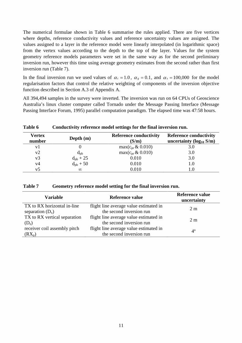
Figure A.1 Schematic representation of the framework for GA-LEI inversion of TEMPEST AEM data. Red elements are the unknowns to be solved for.............. 23

1

1 Introduction

This report describes the geophysical inversion of airborne electromagnetic (AEM) survey data to produce subsurface electrical conductivity predictions. The AEM data were acquired by Fugro Airborne Surveys (FAS) during 2001 with the TEMPEST system. The Billabong Creek survey area is located to the north of Albury and to the southwest of Wagga Wagga in New South Wales, Australia (Figure 1). The survey was funded by the Murray Darling Basin Commission under its Strategic Investigations and Education (SI&E) Program, as part of Airborne Geophysics - SI&E Project D2018. The project was a pilot testing the relevance of airborne geophysics data for salinity management, and evolved from the National Geophysics Project originally sponsored under the National Dryland Salinity Program. The survey was project managed by the Bureau of Rural Sciences (BRS) with supervision and geophysical advice provided by Geoscience Australia (GA).

Figure 1 Location of the Billabong Creek AEM survey area and downhole conductivity

logs (Phase 1 - magenta; Phase 2 - green).

2

After the initial data acquisition and processing, and before any ground follow up was carried out, three sets of conductivity predictions were generated by FAS. These predictions were generated by conductivity depth transforms (CDT) using the software EmFlow (Macnae et al., 1998) and three-layer layered earth inversions (LEI) using an algorithm described by Sattel (1998).

During 2003 Geoscience Australia (GA) developed a layered earth inversion algorithm which, when applied to the Lower Balonne TEMPEST survey data, significantly improved existing CDT conductivity predictions (Lane et al., 2004a, 2004b). Similar improvements were also reported when the algorithm was applied to the Honeysuckle Creek TEMPEST survey data (Brodie and Fisher, 2008a). Herein we refer to this algorithm as the GA-LEI. On this basis the Bureau of Rural Sciences (BRS) contracted GA to apply similar methods to the Billabong Creek dataset. This report is concerned with the application of the GA-LEI methodology to the Billabong Creek dataset, to generate new conductivity predictions and derived products.

Section 2 provides background information on the development of the GA-LEI algorithm. A full description is supplied in Appendix A for those readers interested in the technical details. Specific non-technical information relating to its application to the Billabong Creek TEMPEST AEM dataset is detailed in Section 5.

2 Background to Geoscience Australia Layered Earth Inversions

As a towed-bird fixed-wing AEM system such as TEMPEST moves along a survey flight line its transmitter (TX) loop and receiver (RX) coils continuously change height and orientation with respect to the ground as well as with respect to each other. The overall geometrical arrangement is known as the system geometry. For TEMPEST, the height of the TX above the ground is dynamically measured with a radar and/or laser altimeter. The TX loop orientation, defined by its pitch and roll angle, is dynamically measured via gyroscopes. However, to date it has been operationally impossible to dynamically measure the relative position and orientation of the RX coils (receiver geometry), for example with laser range finders or GPS technology (Smith, 2001b). The system geometry is an inherent input into the estimation of a conductivity distribution from AEM data, whether this estimation is by a CDT or LEI algorithm. However since the receiver geometry is not measured, it must be either assumed or estimated for use in CDT and LEI algorithms.

TEMPEST data are recorded as a stream of digital samples spaced 13.33 μs (75,000 Hz) apart during both the on-time TX loop current pulses and the off-time. This full waveform recording allows sophisticated digital signal processing techniques to be applied to the data. Thus, as a function of time across the full waveform, the system measures and records the total field response at the RX which is a summation of the primary field response that originates directly from currents in the TX loop and the secondary field (or ground response) that originates from eddy currents induced in the ground. The primary field is dependent on the system geometry, whereas the secondary field is a function of both the system geometry and the ground conductivity. Hence it is the secondary field that is diagnostic of the subsurface conductivity. If the system geometry was known the primary field could be calculated from first principles and subtracted from the total field to leave the diagnostic secondary field. However, since in reality there is no independent knowledge of the primary field, the secondary field or the system geometry, none of the three quantities can be directly isolated.

3

To resolve this impasse, in TEMPEST data processing an attempt is made to decompose the measured total field into primary and secondary components using the knowledge that the secondary field theoretically should approach zero as frequency approaches zero (or as delay time approaches infinity). This decomposition estimates the primary field such that the time domain in-phase component (Smith, 2001a) of the remaining ground response, consisting of sums of exponential basis functions, is minimised (Lane et al., 2004a). Minimising the time domain in-phase component of the ground response is akin to assuming a low conductivity ground model particularly at depth. Once the primary field is estimated, it is then possible to estimate the relative position of the RX coils, assuming that the bird was flying straight and level (i.e. RX in-line with the TX and with zero roll, pitch and yaw).

The assumptions of low ground conductivity and that the RX coils were flying straight and level are thus inherent in the processed data and estimated receiver position before they are input into CDT or LEI algorithms. If these assumptions are not good, the consequence is that conductivity estimates derived from the CDT or LEI algorithms are biased toward ground models with low conductivity at depth and the true conductivity is underestimated at depth. There is a related tendency to compensate for the lack of total conductance, needed to satisfy the data, by overestimating the true conductivity in the near surface. This was observed by Lane et al. (2004b) and has been observed for the Honeysuckle Creek dataset (Christensen, 2003, 2004; Brodie and Fisher, 2008a) when estimates were compared to ground truth data. A further repercussion is that the fitting procedure may not be able to find any layered conductivity structure that is consistent with both the X and Z component data. In this case the CDT or LEI can be run on the X and Z component data separately; however the resulting conductivity models will be different.

The recognition of these limitations led to the work described by Lane et al. (2004a), and has since developed into the GA-LEI algorithm. The rationale behind the algorithm is that since the primary field, secondary field, receiver geometry and ground conductivity cannot be independently isolated, they should at least be treated as components within a single unifying framework. To achieve this, the usual sequentially applied steps of: separating the primary and secondary fields; estimation of receiver geometry; estimation of ground conductivity; and comparison to ground truth information are carried out in one inversion procedure that maximises mutual consistency between each of the items. The measured components of the system geometry and the observed total field data are input into the inversion algorithm, along with a reference model compiled from available ground truth information. The algorithm solves for the unmeasured components of the system geometry and the ground conductivity model. Separation of the primary and secondary fields is unnecessary but can be an incidental output from the procedure.

3 Data acquisition and processing

The AEM data were acquired by Fugro Airborne Surveys (FAS) in August and September 2001, using the TEMPEST system described by Lane et al. (2000). Details of the survey operations are provided in Owers et al. (2001). The survey acquisition parameters are summarised in Table 1.

4

Table 1 Summary of survey data acquisition parameters.

Aircraft: CASA C212-200 Turbo Prop, VH-TEM Date : 31 August to 19 September 2001 Flight line spacing: 200 metres Flight line direction: east-west Line kilometres: 5,522 kilometres Nominal flying height: 115 metres above ground level

Along line sampling: 13.333 μ raw streamed AEM 0.2 seconds (~12 metres) stacked and processed AEM

The initial data processing was also carried out by FAS in 2001. For full details on the processing see Owers et al., (2001). For convenience the steps involved in TEMPEST data processing are summarised below from Lane et al. (2004b).

i. Sferic filtering via wavelet transforms. ii. Stacking with a three-second wide cosine-tapered stacking filter. Output from the stacking

filter was drawn at 0.2-second intervals. iii. Filtering to reject VLF and low frequency noises sources. iv. Deconvolution of the system transfer function and normalisation for the receiver coil

effective area, transmitter loop current, transmitter loop turns and transmitter loop area. v. Convolution of the resultant impulse response with a square waveform.

vi. Windowing to times shown in Table 2. vii. Primary field estimation and removal.

viii. Geometry estimation. ix. Height, pitch, roll and geometry correction (not used in the GA-LEI process).

5

Table 2 Window times and estimated noise levels.

Window Window times (seconds) *Estimated additive noise (fT) Start time End time X-component Z-component

1 0.0000066667 0.0000200000 0.021 0.014 2 0.0000333333 0.0000466667 0.019 0.010 3 0.0000600000 0.0000733333 0.018 0.009 4 0.0000866667 0.0001266667 0.017 0.009 5 0.0001400000 0.0002066667 0.016 0.008 6 0.0002200000 0.0003400000 0.015 0.008 7 0.0003533333 0.0005533333 0.014 0.008 8 0.0005666667 0.0008733333 0.013 0.007 9 0.0008866667 0.0013533333 0.013 0.008 10 0.0013666667 0.0021000000 0.016 0.009 11 0.0021133333 0.0032733333 0.021 0.009 12 0.0032866667 0.0051133333 0.014 0.007 13 0.0051266667 0.0079933333 0.012 0.006 14 0.0080066667 0.0123933333 0.009 0.004 15 0.0124066667 0.0199933333 0.009 0.005 *Estimated multiplicative noise 1.4% 1.3%

*See Section 5.2 for an explanation of the noise estimates.

4 Prior information

4.1 Downhole conductivity logs

Two phases of downhole conductivity logging were carried out in the Billabong creek AEM survey area. In 2002 as part of an air core drilling program (Dent, 2003) 14 holes were logged with an EM39 downhole conductivity probe in a Phase 1 logging program (Figure 1, magenta circles). In 2007 work was undertaken at GA to ascertain if the GA-LEI algorithm could improve upon the initial EmFlow CDT conductivity predictions generated by FAS (Sorensen and Lane, 2007).

This work found that the correlations between GA-LEI inversions of the AEM data and the downhole logs were not good, even after extensive trials of the inversion settings. This is at odds with prior studies, which reported good correlations, for the Lower Balonne survey (Lane et al. 2004b) and Honeysuckle Creek survey (Reid and Brodie, 2006; Brodie and Fisher, 2008a), and a recent 2007 survey of the Lower Macquarie River (Brodie and Fisher, 2008b). After considering the possible reasons for the discrepancy Sorensen and Lane (2007) suggested that measurements from the EM39 downhole conductivity probe used in the Phase 1 logging were in error, and recommended that new logging be undertaken with a different probe.

In May 2007 BRS commissioned a Phase 2 logging program to acquire new logs. Unfortunately the Phase 1 boreholes were not open and available for re-logging, however six new logs were acquired in different bores (Figure 1, green circles). These were acquired with an Auslog downhole conductivity probe by Australian Logging Services. Relatively poor correlations were also noted between the Phase 2 logs and the AEM inversions as well. BRS suggested (Mullen, pers. comm., 2008) that water may have compromised the logging equipment in some of the holes at depth and

6

suggested that data should be truncated below certain depths in three boreholes (GW88535 at 80 m, GW88536 at 60 m, and GW88539 at 62 m).

Given the uncertainty relating to the reliability of both the Phase 1 and Phase 2 downhole logging results, coupled with the small number and close spatial clustering of the Phase 2 logged bores, Geoscience Australia made the assessment that the boreholes could not be used to generate reference models for the inversion of the AEM data. Despite this, a comparison of the inversion results against both Phase 1 and Phase 2 logging is provided in Section 6.1, as it provides the only ground truth data available for making an assessment of the inversion.

4.2 Stratigraphic information

Stratigraphic information on the subsurface of the Billabong Creek AEM survey area was examined to provide some geological context for the inversion process, and to assist with the interpretation of the inversion results and the production of a depth to basement surface (Section 6.5). The following section describes the sources of stratigraphic information and their interpretation. Time constraints did not permit the construction of a 3-dimensional surface from the stratigraphic information as was performed for the Honeysuckle Creek AEM survey (Brodie and Fisher, 2008a).

Stratigraphic information was obtained from geology maps and borehole lithological descriptions. The 1:1 000 000 digital surface geology map by Whitaker et al. (2006) was the main map used, which was based on the work of Adamson et al. (1996) and Tuckwell (1976). The NSW stratotectonic map by Scheibner (1997) and a preliminary bedrock map of the area by Glen et al. (1997) were also used to guide the interpretation of boreholes under sedimentary cover. Lithological descriptions from boreholes were collected from three sources: the Bureau of Rural Sciences (Dent, 2003), the NSW groundwater data archive (2006) from the NSW Government, and mineral exploration bores from Taylor (1983) and Walsh (1996).

The borehole lithological descriptions were interpreted into two simplified stratigraphic classes: sediments and basement. Sediments included the unconsolidated clays, sands and gravels of the Cainozoic Murray Basin and Quaternary deposits, while basement included all fresh and weathered Palaeozoic rocks of the Lachlan Fold Belt. As many of the lithological descriptions were highly ambiguous they did not allow confident interpretations to be made, and the list of boreholes was slowly reduced to only those that were considered reliable. This process resulted in 31 interpreted bores across the AEM survey area: 17 BRS bores, 11 water bores, and 3 exploration bores. These bores were used in the interpretation of a depth to basement surface from the inversion results (Section 6.5).

5 Inversion

5.1 Data

The data input into the inversion algorithm were not the FAS height pitch roll and geometry corrected data that are usually supplied by FAS. It is necessary to input the non-geometry corrected data because the inversion algorithm uses the measured elements of the system geometry and re-estimates three of the non-measured elements of the system geometry.

The processed non-geometry corrected data delivered by FAS represent the estimated secondary field (ground response). They are in fact, the measured total field data minus the estimated primary field. The actual primary field data are not supplied by FAS. Since the inversion algorithm makes

7

use of total field data we had to reconstruct the total field by first recalculating the estimated primary field from (measured, assumed and estimated elements of) the system geometry using dipole formulae (Wait, 1982; Lane et al., 2004b); and then adding the result to the secondary field data (see Appendix A, Section A.2.6). In making the primary field calculation we were consistent with the (reverse) calculation made by FAS processing when estimating the system geometry from the estimated primary field. Specifically that means we: used the gyroscope measured transmitter pitch and roll; assumed the receiver coil assembly’s roll, pitch and yaw was zero; assumed the transmitter to receiver horizontal transverse separation was zero; and used the FAS estimated transmitter to receiver horizontal in-line and vertical separations. We also took into account the different transmitter loop pitch sign conventions used by FAS and the GA-LEI inversion algorithm (Appendix A, Section A.2.1).

5.2 Estimated data errors

To estimate noise in the data we used the additive and multiplicative noise model method developed by Green and Lane (2003). The noise model parameters were those used by Lane et al. (2004b), who derived the parameters from high altitude and repeat line data acquired on the Lower Balonne survey, which was flown by the same TEMPEST aircraft and system immediately before the Billabong Creek survey. The estimated parameters of the noise model are shown in the right hand columns of Table 2 above. The model estimates the standard deviation of the total noise in the kth channel to be,

22 )01.0( Skkk Rmae ××+=

where, ka is the standard deviation of the additive noise in the kth window, m is percentage multiplicative noise over all windows of the component, and S

kR is the secondary field in the kth window.

Additive noise is independent of ground conductivity and caused by factors such as atmospheric sferic activity, electronic noise and vibrational noise. Additive noise levels were determined from fully processed data recorded at high altitude.

Multiplicative noise is related to ground conductivity and is caused primarily by variations in system geometry that are not measured and accounted for. The multiplicative noise model parameter, which is expressed as a percentage of the secondary field response, was estimated from fully processed repeat line data recorded at survey altitude. The FAS height, pitch, roll and geometry corrected data were used for this purpose even though non-geometry corrected data are input into the inversion. The rationale for this is that, since the inversion algorithm uses measured system geometry parameters and solves for unmeasured system geometry parameters, the effect of system geometry variation is largely accounted for. Thus noise model parameters estimated from geometry corrected data are likely to be more representative of inversion misfit errors.

5.3 Model parameters

A multi-layer smooth-model formulation (Constable et al., 1987; Farquharson and Oldenburg, 1993) was used. The conductivity model had 25 layers that increased from 2 m thick at the surface and progressively got 10% thicker with depth. The layer thicknesses are shown in Table 3. During the inversion the layer thicknesses were kept fixed and we inverted for the base ten logarithms of the layer conductivities. The dielectric permittivity and magnetic permeability of each layer are set to that of free space (ε=ε0; μ=μ0).

8

Table 3 Conductivity inversion model layer thicknesses and depths.

Layer number Thickness (m) Depth to top (m) Depth to bottom (m) 1 2.00 0.00 2.00 2 2.20 2.00 4.20 3 2.42 4.20 6.62 4 2.66 6.62 9.28 5 2.93 9.28 12.21 6 3.22 12.21 15.43 7 3.54 15.43 18.97 8 3.90 18.97 22.87 9 4.29 22.87 27.16 10 4.72 27.16 31.87 11 5.19 31.87 37.06 12 5.71 37.06 42.77 13 6.28 42.77 49.05 14 6.90 49.05 55.95 15 7.59 55.95 63.54 16 8.35 63.54 71.90 17 9.19 71.90 81.09 18 10.11 81.09 91.20 19 11.12 91.20 102.32 20 12.23 102.32 114.55 21 13.45 114.55 128.00 22 14.80 128.00 142.81 23 16.28 142.81 159.09 24 17.91 159.09 176.99 25 ∞ 176.99 ∞

We solved for three system geometry parameters; the transmitter to receiver horizontal in-line separation (Dx), the transmitter to receiver vertical separation (Dz), and the pitch of the receiver coil assembly (RXp) as shown in Figure A.1. The other system geometry parameters were set to be either the values as measured by the radar altimeter (transmitter loop height) and gyroscopes (roll and pitch of the transmitter loop); or zero (yaw of the transmitter loop, transmitter to receiver horizontal transverse separation, roll and yaw of the receiver coil assembly).

5.4 Preliminary inversion runs

Three inversions were performed. In the first run we solved for a one layer (half-space) conductivity model and solved for the three system geometry parameters (Dx, Dz, and RXp). The rationale was to use the output of the first inversion run to generate a spatially variable halfspace reference model and first pass geometry estimates as input for a second inversion run, whose results were subsequently used as input for the final inversion run.

In the first inversion run we used a spatially constant 0.010 S/m halfspace reference model as a conductivity reference model. We used the survey wide average of the estimates of the transmitter to receiver separations made in the FAS data processing, and a zero degree receiver pitch for the geometry reference model (Table 4).

9

Table 4 Reference model setting for the first inversion run.

Variable Reference value Reference value uncertainty

halfspace conductivity 0.010 S/m 3 log10 S/m TX to RX horizontal in-line separation (Dx) -122.69 m 2 m TX to RX vertical separation (Dz) -42.14 m 2 m receiver coil assembly pitch (RXp) 0º 4º

Figure 2 Spatially smoothed halfspace conductivity estimate produced from the first

inversion run.

The halfspace conductivity inversion results from the first run were gridded to a 40 m cell size and smoothed using a 15×15 cell (600 m×600 m) moving average kernel (Figure 2). We also calculated the average, along each flight line, of the estimates of three geometry parameters for which we solved.

In the second inversion run we solved for a 25 layer conductivity model as shown in Table 3. The reference model conductivity for all layers was interpolated from the smoothed halfspace conductivity grid estimated in the first inversion run (Figure 2). For the geometry reference values we used the average, calculated over each flight line, of the three geometry parameters (Table 5).

The automated routine described in Section 6.5 (using a conductivity threshold cthresh= 0.030 S/m) was used to estimate the thickness of regolith/depth to basement (dpb) from the results of the second preliminary inversion run. The average conductivity (cpr) of the interval from surface to dpb was then calculated. Both dpb and cpr were gridded to 40 m cell size and spatially smoothed using a 15×15 cell (600 m ×600 m) averaging kernel filter. Images of these quantities, which are used in the final inversion, are shown in Figure 3.

10

Table 5 Reference model setting for the second inversion run.

Variable Reference value Reference value uncertainty

conductivity of the 25 layers interpolated from smoothed halfspace conductivity grid estimated in the first

inversion run (Figure 2) 3 log10 S/m

TX to RX horizontal in-line separation (Dx)

flight line average value estimated in the first inversion run 2 m

TX to RX vertical separation (Dz)

flight line average value estimated in the first inversion run 2 m

receiver coil assembly pitch (RXp)

flight line average value estimated in the first inversion run 4º

Estimated regolith conductivity (cpr) Estimated regolith depth (dpb)

Figure 3 Spatially smoothed estimates of the average conductivity and thickness of the regolith produced from the second preliminary inversion run.

5.5 Final inversion run

The rationale behind the production of the smoothed grids of the automated estimated depth to basement (db) and average conductivity of the regolith (cpr) from the second preliminary inversion run was to introduce spatial context, which is not offered by a survey wide average conductivity profile, to the reference and starting models for the final inversion run.

We used a conductivity reference model that started from the maximum of cpr and 0.010 (S/m) at the surface and continued at this value until depth dpb. Below depth dpb it was tapered back to the basement conductivity of 0.010 S/m over a 25 m interval. This is demonstrated schematically by Figure 4 which shows two possible reference model examples where db = 40 m and cpr= 0.200 S/m (red profile) and db = 10 m and cpr= 0.040 S/m (blue profile).

The (logarithmic) linear tapering of the reference conductivity profile from the estimated regolith conductivity back to the basement conductivity over 25 m prevented non-smooth starting and reference models occurring, which are not ideal because they can cause conflict between reference model and smoothness constraints and lead to inversion instability.

11

The numerical formulae shown in Table 6 summarise the rules applied. There are five vertices where depths, reference conductivity values and reference uncertainty values are assigned. The values assigned to a layer in the reference model were linearly interpolated (in logarithmic space) from the vertex values according to the depth to the top of the layer. Values for the system geometry reference models parameters were set in the same way as for the second preliminary inversion run, however this time using average geometry estimates from the second rather than first inversion run (Table 7).

In the final inversion run we used values of 0.1=cα , 1.0=gα , and 000,100=sα for the model regularisation factors that control the relative weighting of components of the inversion objective function described in Section A.3 of Appendix A.

All 394,494 samples in the survey were inverted. The inversion was run on 64 CPUs of Geoscience Australia’s linux cluster computer called Tornado under the Message Passing Interface (Message Passing Interface Forum, 1995) parallel computation paradigm. The elapsed time was 47:58 hours.

Table 6 Conductivity reference model settings for the final inversion run.

Vertex number Depth (m) Reference conductivity

(S/m) Reference conductivity uncertainty (log10 S/m)

v1 0 max(cpr & 0.010) 3.0 v2 dpb max(cpr & 0.010) 3.0 v3 dpb + 25 0.010 3.0 v4 dpb + 50 0.010 1.0 v5 ∞ 0.010 1.0

Table 7 Geometry reference model setting for the final inversion run.

Variable Reference value Reference value uncertainty

TX to RX horizontal in-line separation (Dx)

flight line average value estimated in the second inversion run 2 m

TX to RX vertical separation (Dz)

flight line average value estimated in the second inversion run 2 m

receiver coil assembly pitch (RXp)

flight line average value estimated in the second inversion run 4º

12

Figure 4 Schematic representation of two possible conductivity reference models used

in the final inversion run. The red profile represents db = 40 m and cpr= 0.200 S/m, and the blue profile represents db = 10 m and cpr= 0.040 S/m.

6 Post inversion processing

6.1 Comparison with downhole logs

The inversion results have been compared to the downhole conductivity logs acquired in the survey area. For each borehole the downhole log and the inverted conductivity profile from the closest AEM sample is plotted in Figure 5 (Phase 1), Figure 6 (Phase 1 continued) and Figure 7 (Phase 2). The distance from the borehole to the closest AEM sample is also shown on the plots.

13

Figure 5 Comparisons (part 1) of downhole conductivity logs from the Phase 1 logging

and GA-LEI estimated conductivity.

14

Figure 6 Comparisons (continued) of downhole conductivity logs from the Phase 1 logging and GA-LEI estimated conductivity.

15

Figure 7 Comparisons of downhole conductivity logs from the Phase 2 logging and GA-LEI

estimated conductivity.

Figure 8 shows scatter plot comparisons between conductivities measured by downhole conductivity logging and estimates from FAS’s Sattel three layer inversion (top left), FAS’s EmFlow CDI (top right) and the GA-LEI inversion (bottom right). Each point represents the average conductivity over 5 m depth intervals intersected in the boreholes. Note that the black diagonal line is not a line of best fit, but is the line of 1:1 correspondence along which the scatter points would ideally lie if the downhole logs were error free.

Despite the questionable value of the downhole conductivity logs (Section 4.1), they remain the only ground truth data available for assessing the inversion results. The assessment is best illustrated by Figure 8, where it can be seen that the GA-LEI results correlate better with the downhole logs (R2 = 0.43) than the previous conductivity estimates produced by the Sattel LEI (R2 = 0.15) and the FAS EmFlow CDI (R2 = 0.29). The assessment in Figure 8 also reveals that the correlation is poorer than what was achieved in previous applications of the GA-LEI method to other AEM surveys (Lane et al., 2004b; Reid and Brodie, 2006; Brodie and Fisher, 2008a, b).

16

Figure 8 Scatter plot comparisons between conductivities measured by downhole

conductivity logging (Phase 1 – blue, Phase 2 – red) and estimates from the three types of conductivity estimates.

6.2 Gridding and microlevelling

The logarithm of all 25 layer conductivities were gridded to a square 40 m cell size from the point located inverted sample data using minimum curvature gridding. These grids were micro-levelled to reduce the effect of artefacts aligned in the flight line direction (Minty, 1991). The decorrugation filter was 1200 m long and 400 m wide and had a tolerance of 1.0 decades. The corrections were applied back to the point located data. The micro-levelled point located data were then gridded, in the same manner as the non micro-levelled data, to produce the final logarithm of layer conductivity grids. These were converted back to linear conductivity. Gridding and microlevelling operations were carried out using the Intrepid Software package (v4.1 Release Build 125- 4/12/2007).

17

6.3 Depth slices

A conductivity depth slice is the average estimated conductivity over a given depth interval. The calculation is a simple weighted average of all the layers that intersect the depth interval. For example by inspection of Table 3 it is straight forward to see that the 5 m to 10 m depth slice would be calculated by,

5105)28.910(4)66.2(3)562.6(

−×−+×+×− tyconductivilayertyconductivilayertyconductivilayer .

Depth slice grids were calculated directly from the micro-levelled layer conductivity grids. The following depth slice grids were produced 0-5 m, 5-10 m, 10-15 m, 15-20 m, 20-30 m, 30-40 m, 40-60 m, 60-80 m, 80-100 m, 100-150 m, and 150-200 m. Example images of four conductivity depth slice grids are shown in Figure 9.

0-5 m slice 10-15 m slice

30-40 m slice 60-80 m slice

Figure 9 Images of four selected conductivity depth slices.

18

Figure 10 Conductivity depth section image for flight line 20040.

6.4 Sections

Conductivity-depth sections were produced for each flight line. These sections are graphical representations of the estimated conductivity in a vertical slice along the line of best fit passing through the flight line. Sections were produced by first applying a five point (~62m) along line median filter to the point located layer conductivity data. These data were then resampled onto the lines of best bit using nearest neighbour interpolation.

We have also included a line on the sections which represents the automatically interpreted basement depth generated by the routine described in Section 6.5. An example section is shown in Figure 10.

6.5 Automatically interpreted depth to basement

A routine was devised for automatically picking a depth to basement surface from the AEM inversion results. The routine began by finding a depth dthresh below which estimates in the inverted vertical conductivity profile fall below a threshold conductivity cthresh for each AEM sample. These were converted to estimated elevations (ethresh) of the basement relative to the Australian height datum (AHD). The flight line profiles of ethresh were then smoothed by sequential application of a 51 point (~625 m) median filter followed by a 101 point (~1225 m) averaging filter. The basement elevation estimates were converted to basement depth estimates. Both basement depths and elevations were gridded to a cell size of 40 m.

We calibrated the result by trialling several choices of the threshold conductivity cthresh and making comparisons of the resultant basement depth estimates with the borehole stratigraphic information described in Section 4.2. We chose to use the trialled value of cthresh = 0.100 S/m, which gave the best correlation between the bore interpreted basement depth and the automatically interpreted basement depth. A scatter plot of the correlations for the final basement depth estimates is shown in Figure 11. Note that the black diagonal line is not a line of best fit, but is the line of 1:1 correspondence along which the scatter points would ideally lie. Images of the final automatically interpreted basement depth and elevation grids are shown in Figure 12.

19

Figure 11 Correlation between the borehole stratigraphy interpreted basement

depths and automated AEM inversion interpreted basement depths.

Estimated basement depth Estimated basement elevation

Figure 12 Gradient enhanced images of the estimated depth and elevation of the basement surface grids using the automated basement picking routine. Gradient enhancement is by an east-west sun angle kernel.

cthresh = 0.140 S/m

20

7 References

Adamson, C.L. and Loudon, A.G., 1966. Wagga Wagga 1:250 000 Geological Sheet SI/55-15, 1st edition, Geological Survey of New South Wales, Sydney.

Brodie, R. and Fisher, A., 2008a. Inversion of TEMPEST AEM survey data, Honeysuckle Creek, Victoria. Unpublished report produced by Geoscience Australia for the Bureau of Rural Sciences.

Brodie, R. and Fisher, A., 2008b. Inversion of TEMPEST AEM survey data, Lower Macquarie River, New South Wales. Unpublished report produced by Geoscience Australia for the Bureau of Rural Sciences.

Christensen A., 2003. Calibration of Electromagnetic Data. In: Dent DL (Editor). MDBC Airborne Geophysics Project - Final Report, Consultancy D2018, December 2002, 17-33.

Christensen, A., 2004. Calibration of Honeysuckle Creek conductivity-depth imaging. Geological Survey of Victoria Unpublished Report 2004/1.

Constable, S.C., Parker, R.L. and Constable, C.G., 1987. Occam's inversion: a practical inversion method for generating smooth models from electromagnetic sounding data. Geophysics, 52, 289-300.

Dent, D.L., 2003. MDBC Airborne Geophysics Project: Final Report. Consultancy D 2018. Bureau of Rural Sciences, Canberra.

Farquharson, C.G., and Oldenburg, D.W., 1993. Inversion of time domain electromagnetic data for a horizontally layered earth. Geophysical Journal International, 114, 433–442.

Glen, R., Fleming, G., Lewis, P. and Raphael, N., 1997. Geological digital data package for the Discovery 2000 Albury Project area, Version 1. Geological Survey of New South Wales, Sydney, Australia. Published on CD-ROM.

Green, A., and Lane, R., 2003. Estimating noise levels in AEM data. Extended Abstract, ASEG 16th Geophysical Conference and Exhibition, February 2003, Adelaide.

Lane, R., Brodie, R., and Fitzpatrick A., 2004a. A revised inversion model parameter formulation for fixed wing transmitter loop – towed bird receiver coil time-domain airborne electromagnetic data. Extended Abstract, ASEG 17th Geophysical Conference and Exhibition, Sydney 2004.

Lane, R., Brodie, R., and Fitzpatrick A., 2004b. Constrained inversion of AEM data from the Lower Balonne Area, Southern Queensland, Australia. CRC LEME open file report 163.

Lane, R., Green, A., Golding, C., Owers, M., Pik, P., Plunkett, C., Sattel, D. and Thorn, B., 2000. An example of 3D conductivity mapping using the TEMPEST airborne electromagnetic system. Exploration Geophysics, 31: 162-172.

Macnae, J.C., King, A., Stolz, N., Osmakoff, A. and Blaha, A., 1998. Fast AEM data processing and inversion. Exploration Geophysics, 29, 163-169.

21

Message Passing Interface Forum, 1995. MPI: A Message-Passing Interface standard (version 1.1). Technical report. http://www.mpi-forum.org. 1.3.

Minty, B.R.S., 1991. Simple micro-levelling for aeromagnetic data. Exploration Geophysics, 22, 591-592.

Mullen , I, 2008. Email correspondence concerning Billabong Creek downhole logging from Ian Mullen (BRS) to Ross Brodie (GA) on 12 February 2008.

Owers, M., Sattel, D., and Stenning, L., 2001. Billabong Creek, New South Wales, TEMPEST Geophysical Survey: acquisition and processing report. Unpublished Fugro Airborne Surveys report to the Bureau of Rural Sciences.

Reid, J.E., and Brodie, R.C., 2006. Preliminary inversions of Honeysuckle Creek airborne electromagnetic data: Comparison with borehole conductivity logs and previously derived conductivity models. Unpublished report produced by Geoscience Australia for the Bureau of Rural Sciences.

Sattel, D., 1998. Conductivity information in three dimensions. Exploration Geophysics, 29, 157-162.

Scheibner, E., 1997. Stratotectonic map of New South Wales, Scale 1:1 000 000. Geological Survey of New South Wales, Sydney.

Smith, R.S., 2001a. On removing the primary field from fixed wing time-domain airborne electromagnetic data: some consequences for quantitative modelling, estimating bird position and detecting perfect conductors. Geophysical Prospecting, 49, 405-416.

Smith, R.S., 2001b. Tracking the transmitting-receiving offset in fixed-wing transient EM systems: methodology and application. Exploration Geophysics, 32, 14-19.

Sorensen, C. and Lane, R., 2007. Billabong Creek: Notes on reprocessing of the AEM data using GALEI. Unpublished report produced by Geoscience Australia for the Bureau of Rural Sciences.

Taylor, B.G., 1983. Exploration licences 1784, 1800, 1919 and 1954 Albury/Wagga Wagga, New South Wales: Final Report, period ended – 2nd June, 1983. Samedan Oil Corporation, Samedan Australia. Geological Survey of NSW Company Report 1983/299.

Tuckwell, K.D., 1976. Jerilderie 1:250 000 Geological Sheet SI/55-14, 2nd edition, Geological Survey of New South Wales, Sydney.

Wait, J.R., 1982, Geo–electromagnetism. Academic Press Inc.

Walsh, J.T., 1996. Final report on exploration licences 4625-8 and 4780 (SI 55-13,14). North Limited. Geological Survey of NSW Company Report 1996/139.

Whitaker, A.J., Raymond, O.L., Liu, S., Champion, D.C., Stewart, A.J., Retter, A.J., Percival, D.S., Connolly, D.P., Phillips, D., and Hanna, A.L., 2006. Surface geology of Australia 1:1,000,000 scale, eastern States [Regional GIS dataset], Geoscience Australia, Canberra.

22

Appendix A – GA-LEI Inversion of TEMPEST Data

A.1 Introduction

The GA-LEI inversion program is capable of inverting data from most airborne time-domain AEM systems. It has the capability of inverting for layer conductivities, layer thicknesses, and system geometry parameters, or some subset of these. There are options to use a multi-layer smooth-model formulation (Constable et al., 1987) or a few-layer blocky-model formulation (Sattel, 1998). For the sake of simplicity, only the aspects of the algorithm that are relevant to the inversion of TEMPEST data using a multi-layer smooth-model are described.

TEMPEST data consist of a collection (tens of thousands to millions) of point located multi-channel samples acquired at 0.2 s (approximately 12 m) intervals along survey flight lines. The algorithm independently inverts each sample. The data inputs to the inversion of each sample are the observed total (primary plus secondary) field X-component and Z-component data. Auxiliary information input into the algorithm are the measured and assumed elements of the system geometry, the thicknesses of the layers, and prior information on the unmeasured elements of the system geometry and ground conductivity. The unknowns solved for in the inversion (outputs) are the electrical conductivity of the layers and the unmeasured elements of the system geometry.

Since each sample is inverted independently, the user may elect to invert all samples or some subset of them. The inversion of each sample results in an estimate of a one dimensional (1D) conductivity structure associated with that sample. Each estimated 1D conductivity structure, although theoretically laterally constant and extending infinitely in all directions, is only supported by the data within the system footprint which is approximately a square of side length 470 m centred about the sample point (Reid and Vrbancich, 2004). So by progressively inverting all the samples and stitching together the resultant 1D conductivity structures a depiction of the overall laterally variable 3D conductivity structure is built up.

A.2 Formulation

Figure A.1 shows the overall framework under which the inversion of a single airborne sample is carried out. The elements of the figure are progressively described in the following sections.

A.2.1 Coordinate system

Since each sample is inverted separately the coordinate system is different for the inversion of each sample. A right handed xyz Cartesian coordinate system is used. The origin of the coordinate system is on the Earth’s surface directly below the centre of the transmitter loop. The x-axis is in the direction of flight of the aircraft at that sample location, the y-axis is in the direction of the left wing and the z-axis is directed vertically upwards.

A.2.2 System geometry

The centre of the transmitter loop is located at (0, 0, TXh). Roll of the transmitter loop (TXr) is defined as anti-clockwise rotation, about an axis through (0, 0, TXh) and parallel to the x-axis, so that a positive roll will bring the left wing up. Pitch of the transmitter loop (TXp) is defined as anti-clockwise rotation, about an axis through (0, 0, TXh) and parallel to the y-axis, so that positive pitch will bring the aircraft’s nose down. Yaw of the transmitter loop (TXy) is defined as anti-clockwise rotation, about an axis through (0, 0, TXh) and parallel to the z-axis, so that a positive yaw would turn the aircraft left. However since the x-axis is defined to be in the direction of flight at each

23

sample, the transmitter loop yaw is always zero by definition. The order of operations for calculating the vector orientations is to apply the pitch, roll then yaw rotations respectively.

The position of the receiver coils relative to the transmitter loop is defined by the transmitter to receiver horizontal inline separation (Dx), the transmitter to receiver horizontal transverse separation (Dy), and the transmitter to receiver vertical separation (Dz), The receiver coils are thus located at (Dx, Dy, RXh=TXh+Dz). The receiver coils are always behind and below the aircraft (Dx<0, Dz<0). The receiver coils’ roll (RXr), pitch (RXp) and yaw (RXy) have the same rotational convention as for the transmitter loop except that they are rotations about the point (Dx, Dy, Dz). The receiver coils are always assumed to be located on the y-axis (Dy = 0) and to have zero yaw (RXy = 0). Although this is not in reality the case, the position and orientation is not measured and there is not enough information available to solve for these since Y-component data is not available.

DX

DZ

RXP

c1=10lc1 μ0 ε0 t1=10lt1

c2=10lc2 μ0 ε0 t2=10lt2

cNL=10lcNL μ0 ε0 tNL

= ∞

cNL-1=10lcNL-1 μ0 ε0 tNL-1=10ltNL-1

y-axis

z-axis

x-axis (0,0,0)

… … ... …

TXH

transmitter loop

receiver coils

tow cable

X-component coil

Z-component coil

RXH

horizontal plane

TXPTXR

layer 1

layer NL-1

layer NL1

Figure A.1 Schematic representation of the framework for GA-LEI inversion of TEMPEST AEM data. Red elements are the unknowns to be solved for.

24

Note that transmitter loop pitch data supplied by Fugro Airborne Surveys in processed TEMPEST data uses the convention where a positive transmitter pitch is nose up, and accordingly the supplied pitch is reversed in sign before being used in the inversion algorithm.

A.2.3 Layered earth

The layered earth model is independent at each inverted sample location. The layered earth consists of NL horizontal layers stacked on top of each other in layer cake fashion. The kth layer has constant thickness tk and the bottom layer is a halfspace that has infinite thickness (tNL = ∞), extending to infinite depth. The electrical conductivity of the kth layer is ck and it is constant throughout the layer. The magnetic permeability of all layers is assumed to be equal to the magnetic permeability of free space μ0. The dielectric permittivity of all layers is assumed to be equal to the permittivity of free space ε0.

A.2.4 Data

Part of the TEMPEST data processing sequence involves partitioning the total (secondary plus primary) field response that is actually observed into estimates of the unknown primary and secondary field components. Then an estimate of the transmitter to receiver horizontal in-line and vertical separations Dx and Dz are made from the partitioned primary field component. The procedure uses the measured transmitter pitch (TXp) and roll (TXr) and assumes the receiver coils are flying straight, level and directly behind the aircraft (Dy=0, RXr=0, RXp=0, and RXy=0). It is the estimated secondary field data, the measured elements of the system geometry (TXh, TXp, TXr, and TXy) and the associated estimates of the unmeasured elements of the system geometry (Dx and Dz) that are delivered to clients. Implicit in the delivered dataset are the assumed elements of the system geometry (Dy=0, RXr=0, RXp=0, and RXy=0). However the estimated primary field data are not delivered to clients.

Since the GA-LEI algorithm makes its own estimate of system geometry as part of the inversion procedure it works with total field data. The input data are the total (primary plus secondary) field X-component and Z-component data. Therefore the total field data are first reconstructed. This is a simple matter of recomputing the primary field from magnetic dipole formulae (Wait, 1983) using the delivered (measured, estimated and assumed) elements of the system geometry then adding them to the delivered secondary field data. Note that the height, pitch, roll and geometry corrected data that are usually delivered as part of TEMPEST datasets are not used because the GA-LEI algorithm makes its own estimate of system geometry as part of the inversion procedure.

The reconstructed X-component and Z-component total field data for the kth window are Sk

Pk XXX += and S

kP

k ZZZ += respectively. Here the super scripts P and S represent primary and secondary field components. Since the TEMPEST system has NW = 15 windows, the observed data vector of length ND= 2 NW = 30 used in the inversion is,

TN21N21 ]ZZZXX[X WW =obsd , (1)

where T represents the matrix and vector transpose operator.

Errors on the data are calculated outside of the program and input along with the data. Errors are assumed to be uncorrelated and Gaussian distributed. They are estimated as standard deviations of the Gaussian error distribution for each window and receiver component. Typically errors are calculated from the parameters of an additive plus multiplicative noise model (Green and Lane, 2003). Parameters of the noise model are determined from analysis of high altitude and repeat line

25

data. If errkX and err

kZ , represent the estimated standard deviation of the error in the kth window of the X- component and Z-component data respectively then the data error vector of length ND=30 is,

TerrN

err2

err1

errN

err2

err1 ]ZZZXX[X WW =errd . (2)

A.2.5 Model parameterisation

The unknown model parameter vector (m) to be solved for in the inversion is comprised of earth model parameters and system geometry model parameters.

For the inversion of the TEMPEST dataset described here we choose to use a multi-layer smooth-model formulation (Constable et al., 1987) rather than a few-layer blocky-model formulation (Sattel, 1998). Therefore we solve for the NL conductivities of the layers but not the thicknesses. The layer thicknesses are inputs into the algorithm and are kept fixed throughout. To maintain positivity of the layer conductivities we actually invert for the base ten logarithms of the conductivities of each layer.

We solve for NG=3 system geometry parameters; the transmitter to receiver horizontal in-line separation (Dx), the transmitter to receiver vertical separation (Dz), and the pitch of the receiver coil assembly (RXp).

The unknown model parameter vector of length NP=NG + NL to be solved for is the concatenated vector of log base ten layer conductivities T

N10210110 ]clog clog c[log L=lc and the geometry parameters T]RX D [D pzx=g , such that,

TpzxN10210110 ]RX D D clog clog c[log ] |[ L== glcm (3)

A.2.6 Forward model and derivatives

The forward model is the non-linear multi-valued function,

)]|()|()|([)( 21 pmpmpmmf DNfff = , (4)

which for a given a set of model parameters (m) calculates the theoretical total field data equivalent to that which would be produced for an ideal system, after the measurement and transformation by the data processing steps (Lane et al., 2000). Here each )|( pmkf is a function, not only of the layer conductivities and system geometry parameters in the inversion model vector m, but also of several other fixed parameters p (layer thicknesses; transmitter height, pitch and roll; receiver roll and yaw, transmitter to receiver horizontal transverse separation; system waveform and window positions etc.).

The implementation of (4) is based upon the formulation of Wait (1982) in which he develops the frequency-domain expressions for the magnetic fields due to vertical and horizontal magnetic dipole sources above a horizontally layered medium. The formulation does not account for the contribution due to displacement currents. We also assume that effects of dielectric permittivity and magnetic susceptibility are negligible compared to electrical conduction, and set each layer’s dielectric permittivity and magnetic permeability to that of free space (εk=ε0; μk=μ0).

The full transient (0.04 s) equivalent square current waveform, to which TEMPEST data are processed, was linearly sampled at 75,000 Hz (3000 samples) and transformed to the frequency domain via fast Fourier transform (FFT). Using Wait’s expressions the secondary B-field was calculated for 21 discrete frequencies between 25 Hz and 37,500 Hz (~6.5 logarithmically equi-spaced frequencies per decade). The inphase and quadrature parts of each component were then

26

individually splined to obtain linearly spaced values at the same frequencies as the nodes of the FFT transformed current waveform. Complex multiplication of splined B-field with the FFT transformed current waveform, followed by inverse FFT, yielded the B field transient response.

The transient was then windowed into the 15 windows by averaging those samples that fell within each window. The primary field, which is constant over all 15 windows, was then computed from Wait’s expressions and added to yield the total field window response in the x-axis and z-axis directions. Finally these were rotated to be aligned with the X-component receiver coil’s axis and Z-component receiver coil’s axis according to the receiver pitch model parameter (RXp) to yield f(m).

The inversion also requires the partial derivatives of f(m) with respect to the model parameters, see equation (19). These were all calculated analytically. For computation of Wait’s coefficient R0, we took advantage of the propagation matrix method (Farquharson et al., 2004) because it is efficient for computation of the partial derivatives with respect to the multiple layer conductivities.

A.2.7 Reference model

The algorithm uses the concept of a reference model (Farquharson and Oldenburg, 1993) to incorporate prior information from downhole conductivity logs or lithologic/stratigraphic logging in order to improve inversion stability and to reduce the trade-off between parameters that are not well resolved independently. Since prior information is not available everywhere within the survey area, and the inversions are carried out in independent sample by sample fashion, it is not plausible to place hard reference model constraints on the model parameters. Instead the reference model provides a soft or probabilistic constraint only. If, from prior information, it is concluded that the likely distribution of the model parameter mk is a Gaussian distribution with mean ref

km and standard deviation unc

km . Then we would define the reference model vector as, Trefrefrefref

Nref2

ref1

ref ]RX D D lc lc [lc L pzx=m (5)

and the reference model uncertainty vector as, Tuncuncuncunc

Nunc2

unc1

unc ]RX D D lc lc [lc L pzx=m (6)

The reference model mean values and uncertainties are inputs to the inversion algorithm and they may be different from sample to sample. The uncertainty values assigned to the reference model control the amount of constraint that the reference model places on the inversion results. A large uncertainty value for a particular parameter implies that the assigned reference model mean value is not well known and thus is allowed to vary a long way from the mean. On the other hand a low uncertainty implies the parameter is well known.

A.3 Objective function

The inversion scheme minimises a composite objective function of the form,

)( vvggccd Φ+Φ+Φ+Φ=Φ αααλ (7)

where dΦ is a data misfit term, cΦ is a layer conductivity reference model misfit term, gΦ is a system geometry reference model misfit term, and vΦ is a vertical roughness of conductivity term. The relative weighting of the data misfit dΦ and the collective model regularisation term,

vvggccm Φ+Φ+Φ=Φ ααα (8)

27

is controlled by the value of regularisation factor λ . The three model regularisation factors cα , gα and sα control the relative weighting within the model regularisation term Φm. The algorithm requires that the α values be set by the user on a application by application basis and they remain fixed throughout the inversion. However the λ is automatically determined within the algorithm by the method described in section A.4.2.

A.3.1 Data misfit

The data misfit Φd is a measure of the misfit, between the data (dobs) and the forward model of the model parameters (f(m)), normalised by the expected error and the number of data. It is defined as,

[ ] [ ])()(

)(12

1

mfdWmfd

mf

−−=

−=Φ ∑

=

obsd

Tobs

N

kerrk

obsk

Dd

D

dd

N (9)

The diagonal ND× ND matrix Wd is,

( )

( )

( )

=

2

22

21

1

1

1

1

errN

err

err

Dd

Dd

d

d

N

W (10)

A.3.2 Conductivity reference model misfit

The conductivity reference model misfit term cΦ is a measure of the misfit, between the logarithmic conductivity model parameters (lc) and the corresponding layer reference model values (lcref) normalised by the layer thicknesses and reference model uncertainty. It is defined as,

[ ] [ ]mmWmm −−=

−=Φ ∑

=

refc

Tref

N

kunck

krefk

L

kc

L

lclclc

NTt

2

1 (11)

where ∑=

=LN

kktT

1

, and the diagonal Np×Np matrix Wc is,

28

( )

( )

( )

( )

=−

−

00

0

2

21

1

22

2

21

1

uncN

N

uncN

N

unc

unc

Lc

L

L

L

L

lct

lct

lct

lct

TN

W .

(12)

Since the bottom layer is infinitely thick, for the purposes of this term we set 22

1 ][ −−= LLL NNN ttt .

A.3.3 System geometry reference model misfit

The system geometry reference model misfit term Φg is a measure of the misfit, between the system geometry model parameters (g) and the corresponding system geometry reference model values (gref) normalised by the number of unknown system geometry parameters (NG=3) and their uncertainty. It is defined as,

[ ] [ ]mmWmm −−=

−=Φ ∑

=

refg

Tref

N

kunck

krefk

Gg

G

ggg

N

2

1

1. (13)

The diagonal NP×NP matrix Wg is,

( )

( )

( )

=

2

2

2

1

1

10

0

00

1

uncp

uncy

uncx

Gg

RX

D

DN

W . (14)

A.3.4 Vertical roughness of conductivity

The vertical roughness of conductivity term Φv is a measure of the roughness of the conductivity profile. It sums the squared second derivative of the logarithm of the vertical conductivity profile,

29

approximated by finite difference over adjacent layer triplets, taking into account the distance between layer centres. The result is normalised by the number of triplets (NL-2) and is defined as,

( )( )

( )( )

mLLm vT

vT

N

k kk

kk

kk

kk

Lv

L

ttlclc

ttlclc

N

=

+

−−

+−

−=Φ ∑

−

= +

+

−

−2

2 1

1

1

11

212121

(15)

where the NL-2×Np matrix Lv is,

( ) ( ) ( ) ( )

( ) ( ) ( ) ( )

+

+−

++−

+

+

+−

++−

+

−=

00

0

1111

1111

21

43433232

32322121

tttttttt

tttttttt

NLvL (16)

Again for the purposes of this term we set 22

1 ][ −−=LLL NNN ttt .

A.4 Minimisation scheme

A.4.1 Linearisation

To minimise the objective function Φ, a linearised gradient based iterative minimisation scheme is used. Collection of the matrix notation misfit term equations (9), (11), (13) and (15) that make up Φ allows us to write,

[ ] [ ][ ] [ ] [ ] [ ][ ]mLLmmmWmmmmWmm

mfdWmfdm

vT

vT

vref

gTref

gref

cTref

c

obsd

Tobs

αααλ +−−+−−

+−−=Φ )()()( (17)

The inversion begins by setting the initial estimate of the model parameters to the reference model (m0=mref). During the nth iteration the current estimate of the model parameters nm is perturbed by the parameter change vector,

nnn mmm −=∆ +1 . (18)

The forward model at the new set of model parameters mn+1 is approximated by a Taylor series expansion about mn, which, after excluding high order terms reduces to,

)()()( 11 nnnnn mmJmfmf −+≈ ++ (19)

where mmfJ ∂∂= )(n is the Jacobian matrix whose ith, jth element is the partial derivative of the ith datum with respect to the jth model parameter evaluated at mn in model space. Making use of (19) and substituting m = mn+1, allows (17) to be rewritten as,

30

[ ] [ ][ ] [ ] [ ] [ ][ ]111111

111 )()()()()(

++++++

+++

+−−+−−

+−−−−−−=Φ

nvT

vT

nvnref

gT

nref

gnref

cT

nref

c

nnnobs

dT

nnnobs

n

mLLmmmWmmmmWmm

mmJmfdWmmJmfdm nn

αααλ

(20)

Since the value of Φ will be minimised when 01 =∂Φ∂ +nm , so we differentiate (20) with respect to mn+1 and set the result to zero and get,

[ ][ ] [ ][ ]111

1

222

)()(20

=++

+

+−−−−

+−−−−=

nvT

vvnref

ggnref

cc

nnnobs

dTn

mLLmmWmmW

mmJmfdWJ n

αααλ

(21)

Collecting terms in the unknown vector mn+1 on the left hand side yields,

[ ][ ] [ ] ref

ccccnnnobs

dTn

nvT

vvggccndTn

mWWmJmfdWJ

mLLWWJWJ

ααλ

αααλ

+++−

=+++ +

)(

)( 1 (22)

Since (22) is in the familiar form of a system of linear equations (A mn+1 = b) we are able to solve for mn+1 using a variety of linea algebra methods. We use Cholesky decomposition.

A.4.2 Choice of the value of λ

An initial value of λ is chosen such that the data and model objective functions will have approximately equal weight. This is automatically realised by computing the ratio of the data and model objective functions, from the reference model perturbed by 1%, and computing the ratio of the data and model misfits,

)01.1())01.1((

0

0

mmf

×Φ×Φ

=m

dstartλ . (23)

Then at each iteration the inversion employs a 1D line search where, in solving for 1+nm in (22) different values of λ are trialled, until a value of nλ is found such that,

))((7.0))(( arg1 nd

ettdnd mfmf Φ×=Φ≈Φ + , (24)

thus reducing dΦ to 0.7 of its previous value.

A.4.3 Convergence criterion

The iterations continue until the inversion terminates when one of the following conditions is encountered;

dΦ reaches a user defined minimum value 1min =Φd ;

dΦ has been reduced by less than 1% in two consecutive iterations;

dΦ can no longer be reduced; or

the number of iterations reaches a maximum of 100 iterations.

A.5 References Constable, S.C., Parker, R.L. and Constable, C.G., 1987. Occam's inversion: a practical inversion

method for generating smooth models from electromagnetic sounding data. Geophysics, 52, 289-300.

31

Farquharson, C.G., and Oldenburg, D.W., 1993. Inversion of time domain electromagnetic data for a horizontally layered earth. Geophysical Journal International, 114, 433–442.

Farquharson, C. G., D. W. Oldenburg, and P. S. Routh, 2004, Simultaneous 1D inversion of loop-loop electromagnetic data for magnetic susceptibility and electrical conductivity. Geophysics, 68, 1857–1869.

Green, A., and Lane, R., 2003. Estimating Noise Levels in AEM Data. Extended Abstract, ASEG 16th Geophysical Conference and Exhibition, February 2003, Adelaide.

Lane, R., Green, A., Golding, C., Owers, M., Pik, P., Plunkett, C., Sattel, D. and Thorn, B., 2000. An example of 3D conductivity mapping using the TEMPEST airborne electromagnetic system. Exploration Geophysics, 31: 162-172.

Reid, J.E., and Vrbancich, J., 2004. A comparison of the inductive-limit footprints of airborne electromagnetic configurations. Geophysics, 69, 1229–1239.

Sattel, D., 1998, Conductivity information in three dimensions. Exploration Geophysics, 29, 157–162.

Wait, J.R., 1982, Geo–electromagnetism. Academic Press Inc.