Embed Size (px)
Citation preview

����������������
�������������������������������������������������� �������������������������������������������������� ������������������������������������� ���������������������������������������������������������
������������������������� �������������������������������������� ��������������� ������ � �������������
����
������
�����
�
�������
������������������������
���� ��������������
���������
������
������
��������������������������������������������
����������������������������������� ������
��������������
������ � �������������

��������� ��������������� �������������������� �����������
������������� �������������������������
�������������
������� ������� ����������������� �������� ������ ���� ����!�����"#��������$��������������%�&��������� ��������������������� ����!���������!����%�������������'����������������������� �������(�������������������)� ������ �������������*����+,�
������������������������������������ �����!���� �������"����� ���������

����������#���������- ������ �.�����/��0��
�������"�����- ������ �.�����/��0��
$���� ������%� �����- ������ �1�� ���2�� ����%�3�����.�������!��4 �� �����#���5��������4��%�6 �����- ������ �7�����8 ����� %���� �������1��9�%�8� ����
��������- ������ �2��������/� ���%���� �������!������ �%�8� ����
��������� ��������������� �������������������� �����������
:�1�� �/� ����
;!2.��<=>�?�>��>?)?�>=�;!2.��<=>�?�>��>?)?<>?�"���$�;!!.>1��<��>)��)�;!!.��<��>)��)�"� ���$�;!!.��<��>)�)��"���$�����@��� ,���7.@;!2.@�<=>�?�>��>?)?<>?�
�� ����A��/���+������
6����
�&���������������������'$(�()�%**+++',-+++./�����000(�����(��
��������������������� � ������"�������"������������������������ �������������������������
$�&�������������������
����������������� �������������������������������
������������������������������������������ !�"�����#"!�!��$�%&'()*%+�
,���"���������� �����������
!�����������& ����"+����������)*%+� ���������"������%,����������)*%+�
$�� ����������&����#�����"1"���2%%�$�������)*%+� ���#��#�#�������
!���#���� �������"�����������1�� ���3���#������������2
�&������!��������������������������������������������������������������������������-�!�������.���������������������������/����0���1����������.��������������23���������������3�����������������������������������-�!�������������������������������������������������������������������������������������������4����2���-��������������������������������������������������������������������� ����������������4��2��������4�����������������������������������������2������������.����������������������4��������������������5��-��!���������������������������������������������3�������!�6������������5����������������������7��������������������-�!�����������������������.��������������������������������������1�������������3�1��������������2�����������5�����������5���-�!�������������5�������������������������������-������������������������8"��������������������4����2����������������������������������������������-�9�������������������������������������������������������������������������������������������4���������������������������������������������������������������4����2���-�
4��0��"� ���������������������4������������������������������4�����.�������������4�8"4���������������
�) 1������"2&:;3&<)3'*3<,<'3;� �) 1�"�2&:;3&<)3'*3<,<:3<�
�� -�%:&&3,&+,� �� 1������"2%:&&3,&+,� �� 1�"�2%:&&3,&,)�
������������&������������6�� �����������������#������6�� 5���)*%+�
$�#��%),� �������=((���-�(�"$=�>$=&:;3&<)3'*3<,<:3<�

��������� 6�����-���������'$�**+++'+++./�����000(�����(��
��7�86���������������96��:�7��8���� �7??������?������������?����������������6�������������
;��7����8�/��������������6�6��6����
57��77: ��������6���@��������������������������
���8������������������������������������� !�"�����#"!�!��$�%&'()*%+�
���7� ����� ��������66��
46��7��8����7����� *+-*&-)*%+� 96��:��6��6%,-%)-)*%+�
;��7��������� �:��6 ���6��6%%-%%-)*%+� 4����#��������
!���#����� 5�"����� 6�6��:�7��8�1����������-���3�����������77����2
��������� 6!?�?��?��A�6��@��6?�����������������������6������������6??������?����������������6������@�����������?-�/����������?�A������6�����6���6�����?�����6����@�����������?����@������������������@��6������������������������6����-�$?������?�����������������?�����������������������������?������??��6���������������-�!������������ ������������3���������������������?6������6����������������6?������������6���66��4�@��6������6����������������������������6���6�����?�����6����@�����������??-�����?6���������??��!�6���3���������������@����@�������@���7����3���������������������������?�������������������������?-� �������?�6?���??�����?������������������������6������������������������������������������������������-��������������?���������������@���6?����??����@��������4�@����@�������@�������?��������6��������6�������������@���������8"3����������������4��?�?�����6���6�����������������������-�B��66��@���������������?�����66�������������??����������������������������������4����������������������������������6����������������6??�������������-�
����������6??������?����������4������������������4�6���6����?�����6����@�4��8"4���@������
�) 1��������2&:;3&<)3'*3<,<'3;� �) 1�"�2&:;3&<)3'*3<,<:3<�
�� -�%:&&3,&+,� �� 1��������2%:&&3,&+,� �� 1�"�2%:&&3,&,)�
;��7�������77�������6�� $�������77�������6�� 9����)*%+�
���� 66�6%),� �������=((���-�(�"$=�>$=&:;3&<)3'*3<,<:3<�


Preface
This dissertation was written during the years 2008–2013 at the Department of
Mathematics and Systems Analysis, Aalto University. I acknowledge the finan-
cial support for my work from Finnish Doctoral Programme in Computational
Sciences (FICS), Finnish Doctoral Program in Inverse Problems, the Finnish
Cultural Foundation and the Magnus Ehrnrooth foundation.
I am grateful to Professor Nuutti Hyvönen for being such a wholehearted in-
structor and supervisor. His guidance has been invaluable during my doctoral
studies. I am also deeply indebted to Professor Simon R. Arridge, Doctor Marta
M. Betcke, Doctor Harri Hakula, Professor Martin Hanke-Bourgeois, and Ms.
Eva Schweickert, with whom I coauthored the articles included in this disser-
tation.
Professor Laurent Bourgeois and Professor Roland Griesmaier are acknowl-
egded for the rigorous pre-examination of this dissertation. Furthermore, I am
honored that Professor Bastian von Harrach has agreed to act as my opponent.
Finally, I express my gratitude to my family for all the encouragement and
support they have given me.
Espoo, November 7, 2013,
Lauri Harhanen
1

Preface
2
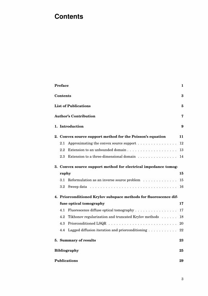
Contents
Preface 1
Contents 3
List of Publications 5
Author’s Contribution 7
1. Introduction 9
2. Convex source support method for the Poisson’s equation 11
2.1 Approximating the convex source support . . . . . . . . . . . . . . . 12
2.2 Extension to an unbounded domain . . . . . . . . . . . . . . . . . . . 13
2.3 Extension to a three-dimensional domain . . . . . . . . . . . . . . . 14
3. Convex source support method for electrical impedance tomog-
raphy 15
3.1 Reformulation as an inverse source problem . . . . . . . . . . . . . 15
3.2 Sweep data . . . . . . . . . . . . . . . . . . . . . . . . . . . . . . . . . 16
4. Priorconditioned Krylov subspace methods for fluorescence dif-
fuse optical tomography 17
4.1 Fluorescence diffuse optical tomography . . . . . . . . . . . . . . . . 17
4.2 Tikhonov regularization and truncated Krylov methods . . . . . . 18
4.3 Priorconditioned LSQR . . . . . . . . . . . . . . . . . . . . . . . . . . 20
4.4 Lagged diffusion iteration and priorconditioning . . . . . . . . . . . 22
5. Summary of results 23
Bibliography 25
Publications 29
3

Contents
4
List of Publications
This thesis consists of an overview and of the following publications which are
referred to in the text by their Roman numerals.
I Lauri Harhanen and Nuutti Hyvönen. Convex source support in half-plane.
Inverse Problems and Imaging, 4(3), 429–448, 2010.
II Harri Hakula, Lauri Harhanen and Nuutti Hyvönen. Sweep data of electri-
cal impedance tomography. Inverse Problems, 27(11), 115006 (19pp), 2011.
III Martin Hanke, Lauri Harhanen, Nuutti Hyvönen and Eva Schweickert.
Convex source support in three dimensions. BIT Numerical Mathematics,
52(1), 45–63, 2012.
IV Simon R. Arridge, Marta M. Betcke and Lauri Harhanen. A priorcondi-
tioned LSQR algorithm for linear ill-posed problems with edge-preserving
regularization. arXiv:1308.6634, 22pp, 2013.
5

List of Publications
6
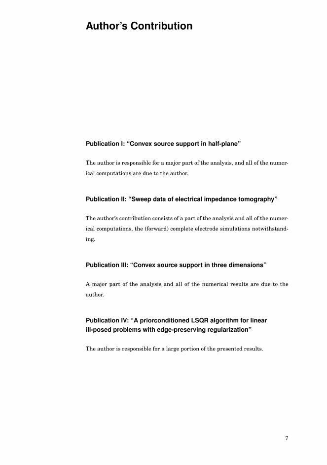
Author’s Contribution
Publication I: “Convex source support in half-plane”
The author is responsible for a major part of the analysis, and all of the numer-
ical computations are due to the author.
Publication II: “Sweep data of electrical impedance tomography”
The author’s contribution consists of a part of the analysis and all of the numer-
ical computations, the (forward) complete electrode simulations notwithstand-
ing.
Publication III: “Convex source support in three dimensions”
A major part of the analysis and all of the numerical results are due to the
author.
Publication IV: “A priorconditioned LSQR algorithm for linearill-posed problems with edge-preserving regularization”
The author is responsible for a large portion of the presented results.
7

Author’s Contribution
8
1. Introduction
Imaging methods are not only an integral part of modern medicine, but also
broadly used by the industry in, e.g., non-destructive testing, process tomog-
raphy, and geological exploration. The renowned computerized tomography
(CT), magnetic resonance imaging (MRI), and ultrasonography are accompa-
nied by positron emission tomography (PET), impedance and capacitance to-
mography, elastography, optoacoustic imaging, optical tomography, and several
others. Many of these modalities have both medical and industrial applications
and, from the mathematical point of view, they are inverse problems: The aim
is to deduce some physical quantity from indirect measurements. For example,
CT scanners reconstruct the mass absorption coefficient inside a patient from
x-ray projection images.
Inverse problems can also be described as the complements of direct prob-
lems. Although this dichotomy is not always obvious, the problem considered
direct is often the one where the aim is to solve the result of a law of the na-
ture. These laws are usually expressed as partial differential equations, which
are both local and causal. Consequently, they usually possess favorable stabil-
ity and uniqueness properties. In contrast, inverse problems most often lack
several of the desirable features of direct problems, and hence are significantly
more involved to solve.
This thesis focuses on three problems in diffuse imaging where the measured
physical phenomena is either light or electrical potential. These problems are
characterized by the extreme spreading, or diffusion, occurring in the modeled
field. The proposed methods are devised for inverse source problems: The mea-
sured fields are not directly created by an external device like an x-ray tube
in CT, but they are caused by phenomena that are (at least to some extent)
endogenous to the subject. For example, neural activity in the brain acts as
a source in electroencephalography (EEG), creating electrical potentials which
are measured on the scalp. These measurements are then processed to give
9
Introduction
information on the brain activity.
First, we consider a problem that is related to EEG: the inverse source prob-
lem for the Poisson’s equation in the framework of electrostatics. We provide
two extensions to an algorithm for obtaining certain information, called the con-
vex source support, on the location of an unknown source. Second, we employ
reformulations of two specific cases of electrical impedance tomography (EIT)
where an inclusion in an otherwise homogeneous domain is re-interpreted as
an electrostatic source. The convex source support method is tested on both of
the resulting inverse source problems. Finally, we propose a numerical method
for fluorescence diffuse optical tomography (FDOT), where the light propaga-
tion is modeled using the (stationary) diffusion equation. The proposed method
is directly applicable to other linear inverse problems, as well.
10

2. Convex source support method forthe Poisson’s equation
The article [23] studied the inverse source problem for the Poisson’s equation
Δu = F in D,∂u∂ν
= 0 on ∂D,∫∂D
uds = 0 (2.1)
in a two-dimensional, bounded, convex domain D. Since the distributional,
compactly supported, mean-free source term F is not uniquely determined by
the boundary potential u|∂D , it is essential to consider what can be deduced
about F given u|∂D .
A similar situation is faced also in the framework of inverse source and scat-
tering problems for the Helmholtz equation
(Δ+k2)u = F, (2.2)
coupled with the Sommerfeld radiation condition. Under certain assumptions,
the amplitude u of a time-harmonic wave satisfies (2.2), where k denotes the
wave number and the main interest is the source F [13]. In addition to being
an actual source, F can also represent a secondary source that is induced as
an incoming wave interacts with a scatterer. These inverse problems for the
Helmholtz equation are often studied in an unbounded domain, and the data
are assumed to be so called far field patterns, or the asymptotic behavior of
the outgoing part of u. This corresponds to measurements made far away from
the scatterer. The articles [19, 33, 34, 43, 49] developed the concept of convex
scattering support and a method for its estimation from the corresponding far
field pattern. Described briefly, the convex scattering support is the smallest
convex set which (almost) supports a source compatible with the data.
In [23], the convex scattering support was adapted for the Poisson’s equa-
tion (2.1). Let us denote the related virtual measurement operator by L, that
is, LF := u|∂D with u solving (2.1) for the source F ∈ E ′�(D), where E ′�(D) de-
notes the space of compactly supported, mean-free distributions. Using L, [23]
defined the convex source support of a boundary potential g ∈R (L) as
C g := ⋂LF=g
suppc F, (2.3)
11
Convex source support method for the Poisson’s equation
where suppc F denotes the convex hull of the support of F. Note that the in-
tersection is taken over all the sources that result in the boundary data g. The
convex source support has several interesting properties [23]: In brief, for any
g ∈R (L) and any ε> 0, there exists Fε ∈ E ′�(D) such that LFε = g and
C g ⊂ suppc Fε ⊂ Nε(C g),
where Nε(C g) denotes the open ε-neighborhood of C g. Moreover, C g =� if and
only if g ≡ 0. This means that for any non-trivial boundary potential measure-
ment g, there exists a non-empty unique minimal convex set C g whose any
ε-neighborhood supports a source compatible with the observed potential.
2.1 Approximating the convex source support
The methods for computing approximations of the convex scattering and source
supports for the two-dimensional setting, presented in [33, 34] and [23], rely on
investigating the Fourier coefficients of the measurements. Let us denote the
virtual measurement operator for the Helmholtz equation (2.2) by Lk, that is,
the far field α of the solution u to (2.2) for F is given by α = LkF. In [34], a
Picard test was given for determining if BR , the origin-centered disc of radius
R, contains the convex scattering support of a given far field pattern. To be
precise, there exists a source FR ∈ Hs0(BR) such that α= LkFR if and only if
∞∑j=−∞
|α j|2| j|−2s
∫R0 |Jj(kr)|2rdr
<∞, (2.4)
where α j are the Fourier coefficients of α and Jj represents the Bessel function
of the first kind and of order j.
A very similar test is derived in [23] for the convex source support in the case
where the domain D is the unit disc: With BR ⊂ D and denoting the Fourier
coefficients of g by g j, C g ⊂ BR if and only if
∞∑j=−∞
|g j|2(R+ε)2| j|
<∞ (2.5)
for every ε> 0. Although the tests given in [33, 34] and [23] are derived using
dissimilar techniques, the resulting tests differ only by the scalings applied to
the Fourier coefficients.
Since any practical test can employ only a finite number of Fourier coeffi-
cients, the conditions (2.4) and (2.5) must be approximated. In [34], a simple
thresholding test was introduced as a method for estimating the smallest R for
which (2.4) converges. In contrast, [23] employed a geometrically decreasing
12
Convex source support method for the Poisson’s equation
model log|g j| ≈ m| j|+b for the behavior of the Fourier coefficients as suggested
in [4]. This reduces the summation in (2.5) into a geometric series, from which
we obtain the smallest possible radius R = em.
The above procedures are valid for testing origin centered discs. Naturally,
the methods are viable for detecting sources only if more detailed information
can be extracted. For the Helmholtz equation, this is straightforward: The far
field pattern is actually the restriction of the Fourier transform of F to the circle
of radius k, i.e., α(θ) =F F(kθ), where θ is the polar angle. Hence, the effect of
the translation x → x+c on the far field pattern can be computed by multiplying
α with the function exp(ik|c|cos(θ− c/|c|)).
In the case of the Poisson’s equation, a standard tool from (two-dimensional)
potential theory allows the extraction of further information on the convex
source support of g: By using a suitable Möbius transformation Φ : D → D
from the unit disc onto itself, the original problem (2.1) can be mapped into a
new problem with the transformed source term (|detΦ′|−1F)◦Φ−1 and boundary
data g ◦Φ−1. By applying the test (2.5) to the transformed data, one obtains a
origin-centered, closed disc B containing C (g ◦Φ−1), and, consequently, Φ−1(B)
contains C g. This procedure allows one to test if C g is a subset of any given
closed disc B ⊂ D, leading naturally to the concept of discoidal source support,
which is the intersection of all discs B ⊂ D that contain C g. In practice, one
is only able to use a finite number of Möbius transformations, and hence only
compute an estimate of the discoidal source support.
Domains more complex than a disc can be treated by solving a well-posed
transmission problem in order to obtain a virtual boundary potential on the
boundary of a large enough disc [24]. In principle, this technique also allows
one to obtain more detailed reconstructions of C g since the extended domain
can be arbitrarily large and thus contain larger test discs. However, numerical
reasons impose a limit on the maximum size of usable extended domains [24].
2.2 Extension to an unbounded domain
Publication I considered the inverse source problem for the Poisson’s equation
in an unbounded domain D ⊂ R2. More precisely, the domain is assumed to be
the upper half-plane, and the third condition of (2.1) is replaced with
lim|x|→∞
|u(x)| = 0.
Although [23] assumed boundedness, most of the results actually hold also for
unbounded domains.
13
Convex source support method for the Poisson’s equation
Even though it may seem like the simplest approach, using a single Möbius
transformation Φ to map the half-plane onto the unit disc and then use the
methods from [23] does not result in a desirable algorithm. This is due to the
fact that the preimage of suppc(|detΦ′|−1F) ◦Φ−1 may be non-convex. Hence,
such an algorithm would not approximate the discoidal nor convex source sup-
port of the boundary measurement, although it would carry some information
on the source. Consequently, Publication I employed a family of Möbius trans-
formations to build a technique for approximating the discoidal source support.
The resulting algorithm is able to produce useful reconstructions using obser-
vations only from one side of the examined domain.
2.3 Extension to a three-dimensional domain
Although [23] considered only two-dimensional domains, the main theoreti-
cal results hold also for three spatial dimensions. However, the presented re-
construction algorithm is inherently two-dimensional due to the utilization of
Möbius transformations. Publication III extended the algorithm to three di-
mensions by replacing the Picard test for Fourier coefficients with a test em-
ploying spherical harmonics coefficients and using Kelvin transforms
(Km,bu
)(x) := b
|x−m|u(Im,b(x))
instead of Möbius transformations. Note that even though Im,b, the inversion
by a sphere with center m and radius b, is a conformal mapping in R3, the
composition u ◦Im,b is not harmonic for a harmonic u, whereas Km,bu is. By
choosing suitable spheres, one can construct a family of inversions that map
the unit ball onto itself and use the associated Kelvin transforms to deal with
non-concentric test balls. However, there is a notable difference compared to
the two-dimensional case: Kelvin transforms do not retain the homogeneous
Neumann boundary condition of (2.1), which must be accounted for in the con-
vergence tests.
14
3. Convex source support method forelectrical impedance tomography
The Calderón problem [5], or EIT, refers to the task of determining the bounded
conductivity field σ (with a positive lower bound) from the boundary measure-
ments vf|∂D of the functions vf satisfying the conductivity equation
∇·σ∇v = 0 in D, σ∂v∂ν
= f on ∂D (3.1)
for some mean-free boundary currents f . The problem has received broad inter-
est, and results, both theoretical and practical, have been published in numer-
ous research articles [3, 11, 50]. Our contribution to the Calderón problem con-
sists of two different techniques for applying the convex source support method
in EIT.
3.1 Reformulation as an inverse source problem
First, we choose a feasible boundary current f and denote by v0 the associated
background solution, that is, the function satisfying (3.1) for σ ≡ 1. Assum-
ing that the actual aim is to locate an inclusion in an otherwise homogeneous
medium with unit conductivity, we face a problem where σ= 1+σi and the inho-
mogeneity σi is compactly supported in D. By denoting the difference potential
with w := v−v0, one obtains
Δw =−∇·σi∇v in D,
where v is the solution to (3.1) for σ= 1+σi. The virtual source Fv =−∇·σi∇v
is clearly supported within the support of σi. Hence, methods that are used for
localizing sources can also be utilized for approximating the support of σi.
The combination of this approach with the convex source support was first
published in [24], which assumed that D is a two-dimensional, bounded do-
main. Publications I and III employed the (reformulated) method in a half-
plane and a three-dimensional ball, respectively, using a single boundary cur-
15
Convex source support method for electrical impedance tomography
rent pattern injected with just two electrodes. (It can be thought that a third
electrode is moved along the boundary to measure the potential.)
Because different boundary currents result in different potentials v, it is pos-
sible to obtain further information on the support of σi by using several bound-
ary currents. For each f , one obtains a subset of suppcσi. Therefore, by taking
the union of all such subsets, a larger and thus more accurate approximation
is obtained, cf. [43] for an analogous result in the framework of the Helmholtz
equation.
3.2 Sweep data
Publication II introduced an alternative measurement configuration for EIT
in two dimensions. Instead of using a single current pattern and measuring
the corresponding potential on the whole boundary, we use one fixed and one
moving electrode, apply a unit current between the two electrodes, and measure
the resulting (relative) potential difference. This measurement, considered as a
function of the moving electrode, is called the sweep data. Assuming point-like
electrodes (cf. [22]), the sweep data can be given in the form
ς(y)= (vy −vy0)(y)− (vy −vy
0)(y0), y ∈ ∂D.
The potentials vy and vy0 satisfy (3.1) for σ= 1+σi and σ= 1, respectively, with
the current pattern f = δy −δy0 . Here, the point-like electrodes are modeled as
Dirac delta distributions on ∂D with the singularity lying at the position indi-
cated by the subscript. Obviously, in order to employ such data, one must have
access to the reference data with a homogeneous conductivity either through
time difference imaging or simulations.
In Publication II, we were able to show that the sweep data can, in essence, be
continued as a holomorphic function to the complement of suppσi. Because the
continuation is unique and its real part is harmonic, the convex source support
algorithm can be applied to the sweep data to obtain an estimate for the location
of the inclusion. Since the proof of the harmonic continuation relies strongly on
complex analysis, it is currently not known if the results can be extended to
three spatial dimensions.
Closely related results for the so-called backscatter data of EIT are available
in [25, 26, 27, 30]. The backscatter data can be approximated in practice by
rotating a small probe of two electrodes around D and measuring the voltage
required for maintaining fixed current between them.
16
4. Priorconditioned Krylov subspacemethods for fluorescence diffuseoptical tomography
4.1 Fluorescence diffuse optical tomography
The goal of optical tomography is to determine the optical properties of an ob-
ject by illuminating it with light and measuring the resulting photon density at
the surface. In many applications, the considered media are turbid and, conse-
quently, the propagation of light can be accurately modeled with the diffusion
approximation for the radiative transfer equation. For a diffusion coefficient σ
and an absorption coefficient μ, the photon density u satisfies(−∇·σ∇+μ
)u = q in D,
u+2ζσ∂
∂νu = g on ∂D,
(4.1)
where ζ describes the reflectiveness of the boundary. Illumination can either be
modeled as an inhomogeneous source term q �= 0 or a suitable boundary value
g �= 0. Further details can be found in the extensive review article [1] and the
references therein.
Advances in the design of optical marker substances have drawn attention
to optical molecular imaging, which allows the study of certain functional pro-
cesses and pathologies in living subjects. Its main advantages in comparison
to many other imaging modalities are the non-invasiveness and high sensitiv-
ity that can be achieved at low cost. In contrast, the widely used PET and CT
scanners are expensive and expose the patient to harmful, ionizing radiation.
While several other phenomena can provide contrast [55], we concentrate on
fluorescence diffuse optical tomography (FDOT), where the fundamental idea
is to inject the subject with a fluorescent marker substance that targets the
interesting molecules. When the subject is subsequently illuminated with exci-
tation light field at a wave length λe, the fluorophore, or marker, absorbs light
and re-emits photons at a different wave length λ f . This effectively creates
sources inside the subject. Since the two fields are at different wave lengths, it
17
Priorconditioned Krylov subspace methods for fluorescence diffuse optical tomography
is possible to separate the two photon densities with filters. Important appli-
cations for FDOT include small animal imaging [31, 36, 37, 38, 56] and breast
tumor detection [14, 39, 51].
Often, the fluorophore concentration is small enough to have a negligible ef-
fect on the diffusion and absorption coefficients, and hence the photon density
field uf arising from fluorescence satisfies (4.1) for q = hue and g ≡ 0, where ue
is the excitation photon density field and h is the main object of interest, the
fluorescence yield coefficient. If one knows a priori the diffusion and absorp-
tion coefficients — such knowledge could be obtained using optical tomography
or some other modality — the problem of FDOT is reduced into the following
diffuse, linear inverse source problem: Find the fluorescence yield coefficient h
that results in the measurements MGh, where M is the measurement opera-
tor (see Publication IV) and G maps h to the induced photon density field uf
solving (4.1). This subproblem was the initial target for the results in Publica-
tion IV. However, it became obvious that the same techniques could be used for
other inverse problems as well, shifting the presentation of Publication IV into
a more general direction.
Although the fluorescence yield coefficient is in many applications compactly
supported and localized in the same sense as sources and conductivity inhomo-
geneities in Chapters 2 and 3, it is not currently known if the convex source sup-
port method can be extended to cover FDOT. As noted in [33], the convex scat-
tering support is a flexible theoretical concept, allowing extensions to several
problems. However, it is unclear how to devise an efficient algorithm for com-
puting the convex source support in FDOT. This is because of the absorption,
which, some very exceptional cases notwithstanding, differs from zero every-
where and hence destroys the harmonicity of the photon density field. Conse-
quently, the reconstruction algorithms relying on Möbius transformations and
Kelvin transforms cannot be applied to FDOT. For this reason, we approach
FDOT from an alternative perspective. By adding regularization, the origi-
nal ill-posed problem is replaced with a well-posed one that is (in some sense)
closely related to the original. A treatise on such regularization methods, in-
cluding the two discussed in this section, can be found in [17].
4.2 Tikhonov regularization and truncated Krylov methods
Assuming that the matrix A is a discretization of the compound forward-mea-
surement operator MG, the problem of FDOT is reduced into solving a system
18
Priorconditioned Krylov subspace methods for fluorescence diffuse optical tomography
of ill-posed linear equations
Ax = y, (4.2)
where x and y represent the (discretized) fluorescence yield coefficient and the
available noisy measurements, respectively. Because the measurement and dis-
cretization errors may push y outside the range of A, it is natural to consider
the associated normal equations
AT Ax = AT y. (4.3)
Unfortunately, these equations are even more ill-posed than (4.2) due to the
squaring of A which squares also the condition number of the problem. A com-
mon technique for regaining well-posedness is to use Tikhonov regularization,
that is, to add a penalty term and then seek the minimizer of
‖y− Ax‖2 +αR(x), α> 0. (4.4)
While it is common to use quadratic penalty terms, i.e., R(x) = xTHx or R(x) =‖Lx‖2 because they reduce the minimization of equation (4.4) to a linear prob-
lem, such penalties are somewhat restricted. In fact, many often used penalty
terms such as Perona–Malik anisotropic diffusion [42] and total variation [44]
are non-quadratic. However, the minimization problems corresponding to such
penalties are non-linear and hence significantly harder to solve.
An alternative option is to solve (4.3) using a Krylov subspace method such
as conjugate gradient (CG) [29] and to regularize through early truncation [21].
This approach is equivalent to minimizing ‖y−Ax‖ in a low dimensional Krylov
subspace
Km = span{AT y, AT AAT y, . . . , (AT A)m−1 AT y}.
For comprehensive monographs on the subject, see [46, 52]. Preconditioning
is essential in the successful use of Krylov subspace methods in large scale
problems [2]. Because fast convergence is guaranteed only if the eigenvalues
of the coefficient matrix are clustered (away from zero), preconditioners aim to
make the spectrum narrower by substituting
P−1 AT Ax = P−1 AT y
for (4.3). For well-posed problems this goal is most commonly achieved by tak-
ing the preconditioner P to be an inexpensively invertible, crude approximation
of the coefficient matrix AT A.
For ill-posed problems, convergence and preconditioning are especially intri-
cate. While the rapid decay of eigenvalues indicates a desperate need for pre-
conditioning, it is not practical to try to cluster the eigenvalues since it would
19
Priorconditioned Krylov subspace methods for fluorescence diffuse optical tomography
cause overwhelmingly high amplification of noise. The main objective in Publi-
cation IV was to derive a technique that combines Tikhonov regularization with
Krylov subspace methods in a computationally efficient manner.
4.3 Priorconditioned LSQR
Normal equations (4.3) are encountered so often that a specialized variant of
CG has been derived for them. Although normal equations can be solved using
the standard CG, the squaring of the coefficient matrix makes them consider-
ably more ill-posed than the original equation (4.2). Instead of applying the
Lanczos algorithm [35] to AT A as in CG, analytically equivalent but numer-
ically more stable method is obtained by using the Golub–Kahan bidiagonal-
ization [18] on A. This modified CG algorithm is called LSQR [40, 41], and is
used in Publication IV for solving the fluorescence yield coefficient. Similar to
CG, LSQR performs best when accompanied with a good preconditioner. Since
traditional preconditioning is not applicable to inverse problems, an alternative
stance is taken here.
In [6, 7, 8, 9, 10], inverse problems were considered using the Bayesian para-
digm and smoothness priors. On structured grids, an unnormalized smoothness
prior p is typically defined through the negative logarithm of its probability
density function
− log p(x)∝‖Dx‖2, (4.5)
where D represents a discretized differential operator. On unstructured grids,
differential operators naturally occur in a form leading to priors given as
− log p(x)∝ xTHx. (4.6)
These priors coincide with a family of extensively used quadratic Tikhonov
smoothness penalty terms, cf. Section 4.2. Their motivation arises from the
fact that naive, unregularized solutions to ill-posed problems are typically ex-
tremely oscillating, which usually contradicts with the reality. The strong os-
cillations can be removed by imposing (some degree of) smoothness on the so-
lution.
The definitions (4.5) and (4.6) lead to zero-mean Gaussian priors with the
unscaled covariances (DTD)−1 and H−1, respectively. The corresponding maxi-
mum a posteriori estimate is computed by solving
(AT A+αH)x = AT y, (4.7)
20
Priorconditioned Krylov subspace methods for fluorescence diffuse optical tomography
where we have assumed H = DTD. Note that (4.7) is equivalent to the least-
squares problem ⎛⎝ A�αD
⎞⎠x =
⎛⎝y
0
⎞⎠ .
Motivated by the fact that solving (4.7) for large scale inverse problems requires
iterative methods and preconditioning, [6, 7, 8, 9, 10] introduced priorcondition-
ing: They demonstrated that the inverse of the covariance matrix is a powerful
preconditioner for solving (4.7) with CG. These results have a strong connection
to [8, 20, 28], where differential operators were studied as preconditioners for
ill-posed problems from another perspective.
However, there are some issues with the efficient implementation of the afore-
mentioned priorconditioning schemes on unstructured grids. The least-squares
connection indicates that LSQR would be better suited for solving (4.7) than
CG, but the standard LSQR algorithm [40, 41] assumes that the precondition-
ing is implemented symmetrically, i.e., by effectively substituting AP−1 for A.
On structured meshes, this is achieved by setting P = D, and it is possible
to employ a weighted pseudoinverse if D is non-invertible [16, 32]. On un-
structured grids, symmetric preconditioning of LSQR requires the Cholesky (or
some other suitable symmetric) decomposition of H. Especially for problems
in three spatial dimensions, such a decomposition is prohibitively expensive
to compute. To remedy this issue, Publication IV derived a version of LSQR
which uses an H-weighted inner product instead of the standard one, which al-
lows us to use H as a preconditioner without its Cholesky decomposition. The
factorization-free priorconditioning of LSQR provides a significant advantage:
H is often (smoothness priors, Perona–Malik, total variation, etc.) a discrete
partial differential operator, which can be inverted by efficient solvers designed
specifically for partial differential equations.
Special care must be taken when methods such as multigrid are employed to
compute the effect of multiplying a vector by the inverse of the preconditioner
P. Indeed, CG and LSQR work only with symmetric, constant preconditioners,
but most iterative solvers approximate inverses with matrices that actually
depend also on the vector to which the inverse is applied and not only on the
matrix that is being inverted. Moreover, the approximate inverse may be non-
symmetric even for symmetric matrices. While there exist flexible variants of
Krylov subspace methods that allow non-constant preconditioners [45, 47], they
arguably provide no advantages over the approach taken in Publication IV: A
simple, computationally low-cost single V-cycle multigrid scheme was sufficient
for achieving effective priorconditioning.
21
Priorconditioned Krylov subspace methods for fluorescence diffuse optical tomography
4.4 Lagged diffusion iteration and priorconditioning
For a quadratic penalty R, the minimizer of (4.4) is simple to find by solving a
linear problem giving the critical point of (4.4). For a non-quadratic R, mini-
mization is a non-linear problem and must be solved iteratively. By setting the
gradient of (4.4) to zero, one obtains
AT Ax+α∇R(x)= AT y.
In many cases, including total variation and Perona–Malik regularization, the
gradient of R corresponds to operating on x with an inhomogeneous diffusion
operator whose diffusion coefficient depends on x. The minimizer can be com-
puted, for example, using the lagged diffusivity fixed point iteration [53, 54]. An
equivalent method can also be derived as a Gauss–Newton type algorithm by
using a sparse approximation for the Hessian of R [15]. The resulting method
is given as the iteration
(AT A+αHk)xk+1 = AT y, (4.8)
where the matrix Hk is a discrete diffusion operator with the diffusion coeffi-
cient depending on the previous iterate xk.
The next iterate xk+1 can be efficiently solved from (4.8) using the priorcon-
ditioned LSQR presented in Section 4.3 with Hk acting as the priorconditioner,
see Publication IV. The reason for referring to Hk as priorconditioner instead
of the standard term preconditioner arises from the nature of Hk. Typically,
preconditioners are constructed from knowledge on the matrix that is being in-
verted. In this case, that matrix is AT A. However, Hk does not depend (directly)
on AT A. Instead, Hk represents information about the expected solution. As
the iteration (4.8) progresses, the features of the solution are progressively in-
corporated in the priorconditioner, allowing one to solve xk+1 from (4.8) with a
low number of LSQR iterations.
22

5. Summary of results
Publication I extended the convex source support method to an unbounded do-
main in the framework of inverse source problems for the Poisson’s equation
and EIT. Specifically, the results of [23, 24] were adapted for the half-plane.
The inverse source problem in a half-plane is significantly more ill-posed than
that in the unit disc because the source, in a sense, masks itself more strongly
in the former. In other words, the measurements are carried out only on one
side of the unknown source. Nevertheless, the (appropriately modified) algo-
rithm [23, 24] provides a good approximation for the discoidal source support.
Publication II introduced a novel two-electrode EIT measurement setting
where one electrode resides at a fixed position while the other sweeps along
the boundary of a two-dimensional domain. The difference data for this mea-
surement configuration can be holomorphically continued to the complement
of the support of an inclusion in an otherwise homogeneous domain. Conse-
quently, the convex source support method is applicable to the sweep data. The
performance of the corresponding algorithm was demonstrated using both an
idealized point electrode model and the complete electrode model [12, 48].
Publication III extended the algorithm for computing the convex source sup-
port to a bounded three-dimensional domain. By substituting Kelvin trans-
forms for Möbius transformations, the original discoidal domain of [23, 24] can
be replaced by a ball. The new algorithm was tested in the frameworks of the
inverse source problem for the Poisson’s equation and EIT with a single current
pattern.
Publication IV proposed the use of popular non-quadratic Tikhonov regular-
ization penalties as preconditioners for solving ill-posed least-squares equa-
tions with Krylov subspace methods. In particular, a new variant of LSQR
was derived, allowing efficient use of the proposed preconditioner. The perfor-
mance of the method was demonstrated using a simple deblurring example and
an inverse source problem for FDOT.
23

Summary of results
24
Bibliography
[1] Simon R Arridge and John C Schotland. Optical tomography: forward and inverseproblems. Inverse Problems, 25(123010):123010, 2009.
[2] Michele Benzi. Preconditioning techniques for large linear systems: a survey.Journal of Computational Physics, 182(2):418–477, 2002.
[3] Liliana Borcea. Electrical impedance tomography. Inverse problems, 18(6):R99–R136, 2002.
[4] Martin Brühl and Martin Hanke. Numerical implementation of two nonitera-tive methods for locating inclusions by impedance tomography. Inverse Problems,16(4):1029–1042, 2000.
[5] Alberto P Calderón. On an inverse boundary value problem. In Seminar on Nu-merical Analysis and its Application to Continuum Physics, pages 65–73, Rio deJaneiro, 1980. Brazilian Mathematical Society.
[6] Daniela Calvetti. Preconditioned iterative methods for linear discrete ill-posedproblems from a Bayesian inversion perspective. Journal of computational andapplied mathematics, 198(2):378–395, 2007.
[7] Daniela Calvetti, Debra McGivney, and Erkki Somersalo. Left and right precondi-tioning for electrical impedance tomography with structural information. InverseProblems, 28(5):055015, 2012.
[8] Daniela Calvetti, Lothar Reichel, and Abdallah Shuibi. Invertible smoothing pre-conditioners for linear discrete ill-posed problems. Applied numerical mathemat-ics, 54(2):135–149, 2005.
[9] Daniela Calvetti and Erkki Somersalo. Priorconditioners for linear systems. In-verse problems, 21(4):1397, 2005.
[10] Daniela Calvetti and Erkki Somersalo. Introduction to Bayesian scientific com-puting: ten lectures on subjective computing. Springer New York, 2007.
[11] Margaret Cheney, David Isaacson, and Jonathan C Newell. Electrical impedancetomography. SIAM review, 41(1):85–101, 1999.
[12] Kuo-Sheng Cheng, David Isaacson, Jonathan C Newell, and David G Gisser. Elec-trode models for electric current computed tomography. Biomedical Engineering,IEEE Transactions on, 36(9):918–924, 1989.
[13] David Colton and Rainer Kress. Inverse acoustic and electromagnetic scatteringtheory. Springer-Verlag, Berlin, 1998.
25
Bibliography
[14] Alper Corlu, Regine Choe, Turgut Durduran, Mark A Rosen, Martin Schweiger,Simon R Arridge, Mitchell D Schnall, and Arjun G Yodh. Three-dimensional invivo fluorescence diffuse optical tomography of breast cancer in humans. OpticsExpress, 15(11):6696–6716, 2007.
[15] Abdel Douiri, Martin Schweiger, Jason Riley, and Simon Arridge. An adaptivediffusion regularization method of inverse problem for diffuse optical tomography.In European Conference on Biomedical Optics. Optical Society of America, 2005.
[16] Lars Eldén. A weighted pseudoinverse, generalized singular values, and con-strained least squares problems. BIT Numerical Mathematics, 22(4):487–502,1982.
[17] Heinz Werner Engl, Martin Hanke, and Andreas Neubauer. Regularization ofinverse problems, volume 375. Springer, 1996.
[18] Gene Golub and William Kahan. Calculating the singular values and pseudo-inverse of a matrix. Journal of the Society for Industrial & Applied Mathematics,Series B: Numerical Analysis, 2(2):205–224, 1965.
[19] Houssem Haddar, Steven Kusiak, and John Sylvester. The convex back-scatteringsupport. SIAM Journal on Applied Mathematics, 66(2):591–615, 2005.
[20] Martin Hanke. Regularization with differential operators: an iterative approach.Numerical functional analysis and optimization, 13(5-6):523–540, 1992.
[21] Martin Hanke. Conjugate gradient type methods for ill-posed problems, volume327. Chapman & Hall/CRC, 1995.
[22] Martin Hanke, Bastian Harrach, and Nuutti Hyvönen. Justification of pointelectrode models in electrical impedance tomography. Mathematical Models andMethods in Applied Sciences, 21(06):1395–1413, 2011.
[23] Martin Hanke, Nuutti Hyvönen, Manfred Lehn, and Stefanie Reusswig. Sourcesupports in electrostatics. BIT Numerical Mathematics, 48(2):245–264, 2008.
[24] Martin Hanke, Nuutti Hyvönen, and Stefanie Reusswig. Convex source supportand its application to electric impedance tomography. SIAM Journal on ImagingSciences, 1(4):364–378, 2008.
[25] Martin Hanke, Nuutti Hyvönen, and Stefanie Reusswig. An inverse backscat-ter problem for electric impedance tomography. SIAM Journal on MathematicalAnalysis, 41(5):1948–1966, 2009.
[26] Martin Hanke, Nuutti Hyvönen, and Stefanie Reusswig. Convex backscatteringsupport in electric impedance tomography. Numerische Mathematik, 117(2):373–396, 2011.
[27] Martin Hanke, Nuutti Hyvönen, and Stefanie Reusswig. Erratum: An inversebackscatter problem for electric impedance tomography. SIAM Journal on Math-ematical Analysis, 43(3):1495–1497, 2011.
[28] Per Christian Hansen and Toke Koldborg Jensen. Smoothing-norm precondition-ing for regularizing minimum-residual methods. SIAM journal on matrix analysisand applications, 29(1):1–14, 2006.
26
Bibliography
[29] Magnus R Hestenes and Eduard Stiefel. Methods of conjugate gradients for solv-ing linear systems. Journal of Research of the National Bureau of Standards,49(6):409–436, 1952.
[30] Stefanie Hollborn. Reconstructions from backscatter data in electric impedancetomography. Inverse Problems, 27(4):045007, 2011.
[31] Dax S Kepshire, Summer L Gibbs-Strauss, Julia A O’Hara, Michael Hutchins,Niculae Mincu, Frederic Leblond, Mario Khayat, Hamid Dehghani, SubhadraSrinivasan, and Brian W Pogue. Imaging of glioma tumor with endogenous fluo-rescence tomography. Journal of biomedical optics, 14(3):030501–030501, 2009.
[32] Misha E Kilmer, Per Christian Hansen, and Malena I Español. A projection-basedapproach to general-form Tikhonov regularization. SIAM Journal on ScientificComputing, 29(1):315–330, 2007.
[33] Steven Kusiak and John Sylvester. The scattering support. Communications onpure and applied mathematics, 56(11):1525–1548, 2003.
[34] Steven Kusiak and John Sylvester. The convex scattering support in a backgroundmedium. SIAM journal on mathematical analysis, 36(4):1142–1158, 2005.
[35] Cornelius Lanczos. An iteration method for the solution of the eigenvalue problemof linear differential and integral operators. Journal of Research of the NationalBureau of Standards, 45(4):255–282, 1950.
[36] Abraham Martin, Juan Aguirre, Ana Sarasa-Renedo, Debbie Tsoukatou, Aniki-tos Garofalakis, Heiko Meyer, Clio Mamalaki, Jorge Ripoll, and Anna M Planas.Imaging changes in lymphoid organs in vivo after brain ischemia with three-dimensional fluorescence molecular tomography in transgenic mice expressinggreen fluorescent protein in T lymphocytes. Molecular Imaging, 7(4):157–167,2008.
[37] Vasilis Ntziachristos. Fluorescence molecular imaging. Annual review of biomed-ical engineering, 8:1–33, 2006.
[38] Vasilis Ntziachristos, Christoph Bremer, and Ralph Weissleder. Fluorescenceimaging with near-infrared light: new technological advances that enable in vivomolecular imaging. European radiology, 13(1):195–208, 2003.
[39] Vasilis Ntziachristos, Arjun G. Yodh, Mitchell Schnall, and Britton Chance. Con-current MRI and diffuse optical tomography of breast after indocyanine green en-hancement. Proceedings of the National Academy of Sciences of the United Statesof America, 97(6):2767–2772, 2000.
[40] Christopher C Paige and Michael A Saunders. Algorithm 583: LSQR: Sparselinear equations and least squares problems. ACM Transactions on MathematicalSoftware (TOMS), 8(2):195–209, 1982.
[41] Christopher C Paige and Michael A Saunders. LSQR: An algorithm for sparselinear equations and sparse least squares. ACM Transactions on MathematicalSoftware (TOMS), 8(1):43–71, 1982.
[42] Pietro Perona and Jitendra Malik. Scale-space and edge detection usinganisotropic diffusion. Pattern Analysis and Machine Intelligence, IEEE Trans-actions on, 12(7):629–639, 1990.
27
Bibliography
[43] Roland Potthast, John Sylvester, and Steven Kusiak. A ’range test’ for determin-ing scatterers with unknown physical properties. Inverse Problems, 19(3):533,2003.
[44] Leonid I Rudin, Stanley Osher, and Emad Fatemi. Nonlinear total variation basednoise removal algorithms. Physica D: Nonlinear Phenomena, 60(1):259–268, 1992.
[45] Yousef Saad. A flexible inner-outer preconditioned GMRES algorithm. SIAMJournal on Scientific Computing, 14(2):461–469, 1993.
[46] Yousef Saad. Iterative methods for sparse linear systems. PWS Publishing Com-pany, 1996.
[47] Valeria Simoncini and Daniel B Szyld. Flexible inner-outer Krylov subspace meth-ods. SIAM Journal on Numerical Analysis, 40(6):2219–2239, 2002.
[48] Erkki Somersalo, Margaret Cheney, and David Isaacson. Existence and unique-ness for electrode models for electric current computed tomography. SIAM Jour-nal on Applied Mathematics, 52(4):1023–1040, 1992.
[49] John Sylvester and James Kelly. A scattering support for broadband sparse farfield measurements. Inverse problems, 21(2):759, 2005.
[50] Gunther Uhlmann. Electrical impedance tomography and Calderón’s problem.Inverse Problems, 25(12):123011, 2009.
[51] Stephanie van de Ven, Andrea Wiethoff, Tim Nielsen, Bernhard Brendel, Mar-jolein van der Voort, Rami Nachabe, Martin Van der Mark, Michiel Van Beek,Leon Bakker, Lueder Fels, Sjoerd Elias, Peter Luijten, and Willem Mali. A novelfluorescent imaging agent for diffuse optical tomography of the breast: first clini-cal experience in patients. Molecular Imaging and Biology, 12(3):343–348, 2010.
[52] Henk A van der Vorst. Iterative Krylov methods for large linear systems, vol-ume 13. Cambridge University Press, 2003.
[53] Curtis R Vogel. Computational Methods for Inverse Problems, volume 23. Societyfor Industrial and Applied Mathematics, 2002.
[54] Curtis R Vogel and Mary E Oman. Iterative methods for total variation denoising.SIAM Journal on Scientific Computing, 17(1):227–238, 1996.
[55] Ralph Weissleder and Umar Mahmood. Molecular imaging. Radiology,219(2):316–333, 2001.
[56] Giannis Zacharakis, Hirokazu Kambara, Helen Shih, Jorge Ripoll, Jan Grimm,Yoshinaga Saeki, Ralph Weissleder, and Vasilis Ntziachristos. Volumetric tomog-raphy of fluorescent proteins through small animals in vivo. Proceedings of theNational Academy of Sciences of the United States of America, 102(51):18252–18257, 2005.
28
����������������
�������������������������������������������������� �������������������������������������������������� ������������������������������������� ���������������������������������������������������������
������������������������� �������������������������������������� ��������������� ������ � �������������
����
������
�����
�
�������
������������������������
���� ��������������
���������
������
������
��������������������������������������������
����������������������������������� ������
��������������
������ � �������������