Embed Size (px)
Citation preview

INSTITUTE OF PHYSICS PUBLISHING INVERSE PROBLEMS
Inverse Problems 19 (2003) R27–R83 PII: S0266-5611(03)36025-3
TOPICAL REVIEW
Inverse scattering series and seismic exploration
Arthur B Weglein1, Fernanda V Araujo2,8, Paulo M Carvalho3,Robert H Stolt4, Kenneth H Matson5, Richard T Coates6,Dennis Corrigan7,9, Douglas J Foster4, Simon A Shaw1,5 andHaiyan Zhang1
1 University of Houston, 617 Science and Research Building 1, Houston, TX 77204, USA2 Universidade Federal da Bahia, PPPG, Brazil3 Petrobras, Avenida Chile 65 S/1402, Rio De Janeiro 20031-912, Brazil4 ConocoPhillips, PO Box 2197, Houston, TX 77252, USA5 BP, 200 Westlake Park Boulevard, Houston, TX 77079, USA6 Schlumberger Doll Research, Old Quarry Road, Ridgefield, CT 06877, USA7 ARCO, 2300 W Plano Parkway, Plano, TX 75075, USA
E-mail: [email protected]
Received 18 February 2003Published 9 October 2003Online at stacks.iop.org/IP/19/R27
AbstractThis paper presents an overview and a detailed description of the key logicsteps and mathematical-physics framework behind the development of practicalalgorithms for seismic exploration derived from the inverse scattering series.
There are both significant symmetries and critical subtle differencesbetween the forward scattering series construction and the inverse scatteringseries processing of seismic events. These similarities and differences helpexplain the efficiency and effectiveness of different inversion objectives. Theinverse series performs all of the tasks associated with inversion using the entirewavefield recorded on the measurement surface as input. However, certainterms in the series act as though only one specific task,and no other task, existed.When isolated, these terms constitute a task-specific subseries. We present boththe rationale for seeking and methods of identifying uncoupled task-specificsubseries that accomplish: (1) free-surface multiple removal; (2) internalmultiple attenuation; (3) imaging primaries at depth; and (4) inverting for earthmaterial properties.
A combination of forward series analogues and physical intuition isemployed to locate those subseries. We show that the sum of the four task-specific subseries does not correspond to the original inverse series since termswith coupled tasks are never considered or computed. Isolated tasks areaccomplished sequentially and, after each is achieved, the problem is restartedas though that isolated task had never existed. This strategy avoids choosingportions of the series, at any stage, that correspond to a combination of tasks, i.e.,
8 Present address: ExxonMobil Upstream Research Company, PO Box 2189, Houston, TX 77252, USA.9 Present address: 5821 SE Madison Street, Portland, OR 97215, USA.
0266-5611/03/060027+57$30.00 © 2003 IOP Publishing Ltd Printed in the UK R27

R28 Topical Review
no terms corresponding to coupled tasks are ever computed. This inversion instages provides a tremendous practical advantage. The achievement of a task isa form of useful information exploited in the redefined and restarted problem;and the latter represents a critically important step in the logic and overallstrategy. The individual subseries are analysed and their strengths, limitationsand prerequisites exemplified with analytic, numerical and field data examples.
(Some figures in this article are in colour only in the electronic version)
1. Introduction and background
In exploration seismology, a man-made source of energy on or near the surface of the earthgenerates a wave that propagates into the subsurface. When the wave reaches a reflector, i.e., alocation of a rapid change in earth material properties, a portion of the wave is reflected upwardtowards the surface. In marine exploration, the reflected waves are recorded at numerousreceivers (hydrophones) along a towed streamer in the water column just below the air–waterboundary (see figure 1).
The objective of seismic exploration is to determine subsurface earth properties from therecorded wavefield in order to locate and delineate subsurface targets by estimating the typeand extent of rock and fluid properties for their hydrocarbon potential.
The current need for more effective and reliable techniques for extracting informationfrom seismic data is driven by several factors including (1) the higher acquisition and drillingcost, the risk associated with the industry trend to explore and produce in deeper water and(2) the serious technical challenges associated with deep water, in general, and specificallywith imaging beneath a complex and often ill-defined overburden.
An event is a distinct arrival of seismic energy. Seismic reflection events are catalogued asprimary or multiple depending on whether the energy arriving at the receiver has experiencedone or more upward reflections, respectively (see figure 2). In seismic exploration, multiplyreflected events are called multiples and are classified by the location of the downward reflectionbetween two upward reflections. Multiples that have experienced at least one downwardreflection at the air–water or air–land surface (free surface) are called free-surface multiples.Multiples that have all of their downward reflections below the free surface are called internalmultiples. Methods for extracting subsurface information from seismic data typically assumethat the data consist exclusively of primaries. The latter model then allows one upwardreflection process to be associated with each recorded event. The primaries-only assumptionsimplifies the processing of seismic data for determining the spatial location of reflectors and thelocal change in earth material properties across a reflector. Hence, to satisfy this assumption,multiple removal is a requisite to seismic processing. Multiple removal is a long-standingproblem and while significant progress has been achieved over the past decade, conceptualand practical challenges remain. The inability to remove multiples can lead to multiplesmasquerading or interfering with primaries causing false or misleading interpretations and,ultimately, poor drilling decisions. The primaries-only assumption in seismic data analysisis shared with other fields of inversion and non-destructive evaluation, e.g., medical imagingand environmental hazard surveying using seismic probes or ground penetrating radar. Inthese fields, the common violation of these same assumptions can lead to erroneous medicaldiagnoses and hazard detection with unfortunate and injurious human and environmental

Topical Review R29
Figure 1. Marine seismic exploration geometry: ∗ and � indicate the source and receiver,respectively. The boat moves through the water towing the source and receiver arrays and theexperiment is repeated at a multitude of surface locations. The collection of the different source–receiver wavefield measurements defines the seismic reflection data.
Figure 2. Marine primaries and multiples: 1, 2 and 3 are examples of primaries, free-surfacemultiples and internal multiples, respectively.
consequences. In addition, all these diverse fields typically assume that a single weak scatteringmodel is adequate to generate the reflection data.
Even when multiples are removed from seismic reflection data, the challenges for accurateimaging (locating) and inversion across reflectors are serious, especially when the medium ofpropagation is difficult to adequately define, the geometry of the target is complex and thecontrast in earth material properties is large. The latter large contrast property condition is byitself enough to cause linear inverse methods to collide with their assumptions.
The location and delineation of hydrocarbon targets beneath salt, basalt, volcanics andkarsted sediments are of high economic importance in the petroleum industry today. For thesecomplex geological environments, the common requirement of all current methods for theimaging-inversion of primaries for an accurate (or at least adequate) model of the medium abovethe target is often not achievable in practice, leading to erroneous, ambivalent or misleadingpredictions. These difficult imaging conditions often occur in the deep water Gulf of Mexico,where the confluence of large hydrocarbon reserves beneath salt and the high cost of drilling

R30 Topical Review
(and, hence, lower tolerance for error) in water deeper than 1 km drives the demand for muchmore effective and reliable seismic data processing methods.
In this topical review, we will describe how the inverse scattering series has provided thepromise of an entire new vision and level of seismic capability and effectiveness. That promisehas already been realized for the removal of free-surface and internal multiples. We will alsodescribe the recent research progress and results on the inverse series for the processing ofprimaries. Our objectives in writing this topical review are:
(1) to provide both an overview and a more comprehensive mathematical-physics descriptionof the new inverse-scattering-series-based seismic processing concepts and practicalindustrial production strength algorithms;
(2) to describe and exemplify the strengths and limitations of these seismic processingalgorithms and to discuss open issues and challenges; and
(3) to explain how this work exemplifies a general philosophy for and approach (strategy andtactics) to defining, prioritizing, choosing and then solving significant real-world problemsfrom developing new fundamental theory, to analysing issues of limitations of field data,to satisfying practical prerequisites and computational requirements.
The problem of determining earth material properties from seismic reflection data is aninverse scattering problem and, specifically, a non-linear inverse scattering problem. Althoughan overview of all seismic methods is well beyond the scope of this review, it is accurate tosay that prior to the early 1990s, all deterministic methods used in practice in explorationseismology could be viewed as different realizations of a linear approximation to inversescattering, the inverse Born approximation [1–3]. Non-linear inverse scattering series methodswere first introduced and adapted to exploration seismology in the early 1980s [4] and practicalalgorithms first demonstrated in 1997 [5].
All scientific methods assume a model that starts with statements and assumptionsthat indicate the inclusion of some (and ignoring of other) phenomena and components ofreality. Earth models used in seismic exploration include acoustic, elastic, homogeneous,heterogeneous, anisotropic and anelastic; the assumed dimension of change in subsurfacematerial properties can be 1D, 2D or 3D; the geometry of reflectors can be, e.g., planar,corrugated or diffractive; and the man-made source and the resultant incident field must bedescribed as well as both the character and distribution of the receivers.
Although 2D and 3D closed form complete integral equation solutions exist for theSchrodinger equation (see [6]), there is no analogous closed form complete multi-dimensionalinverse solution for the acoustic or elastic wave equations. The push to develop completemulti-dimensional non-linear seismic inversion methods came from: (1) the need to removemultiples in a complex multi-dimensional earth and (2) the interest in a more realistic modelfor primaries. There are two different origins and forms of non-linearity in the description andprocessing of seismic data. The first derives from the intrinsic non-linear relationship betweencertain physical quantities. Two examples of this type of non-linearity are:
(1) multiples and reflection coefficients of the reflectors that serve as the source of the multiplyreflected events and
(2) the intrinsic non-linear relationship between the angle-dependent reflection coefficient atany reflector and the changes in elastic property changes.
The second form of non-linearity originates from forward and inverse descriptions that are,e.g., in terms of estimated rather than actual propagation experiences. The latter non-linearityhas the sense of a Taylor series. Sometimes a description consists of a combination of these

Topical Review R31
two types of non-linearity as, e.g., occurs in the description and removal of internal multiplesin the forward and inverse series, respectively.
The absence of a closed form exact inverse solution for a 2D (or 3D) acoustic or elasticearth caused us to focus our attention on non-closed or series forms as the only candidates fordirect multi-dimensional exact seismic processing. An inverse series can be written, at leastformally, for any differential equation expressed in a perturbative form.
This article describes and illustrates the development of concepts and practical methodsfrom the inverse scattering series for multiple attenuation and provides promising conceptualand algorithmic results for primaries. Fifteen years ago, the processing of primaries wasconceptually more advanced and effective in comparison to the methods for removingmultiples. Now that situation is reversed. At that earlier time, multiple removal methodsassumed a 1D earth and knowledge of the velocity model, whereas the processing of primariesallowed for a multi-dimensional earth and also required knowledge of the 2D (or 3D) velocitymodel for imaging and inversion. With the introduction of the inverse scattering series for theremoval of multiples during the past 15 years, the processing of multiples is now conceptuallymore advanced than the processing of primaries since, with a few exceptions (e.g., migration-inversion and reverse time migration) the processing of primaries have remained relativelystagnant over that same 15 year period. Today, all free-surface and internal multiples canbe attenuated from a multi-dimensional heterogeneous earth with absolutely no knowledgeof the subsurface whatsoever before or after the multiples are removed. On the other hand,imaging and inversion of primaries at depth remain today where they were 15 years ago,requiring, e.g., an adequate velocity for an adequate image. The inverse scattering subseriesfor removing free surface and internal multiples provided the first comprehensive theoryfor removing all multiples from an arbitrary heterogeneous earth without any subsurfaceinformation whatsoever. Furthermore, taken as a whole, the inverse series provides a fullyinclusive theory for processing both primaries and multiples directly in terms of an inadequatevelocity model, without updating or in any other way determining the accurate velocityconfiguration. Hence, the inverse series and, more specifically, its subseries that performimaging and inversion of primaries have the potential to allow processing primaries to catchup with processing multiples in concept and effectiveness.
2. Seismic data and scattering theory
2.1. The scattering equation
Scattering theory is a form of perturbation analysis. In broad terms, it describes how aperturbation in the properties of a medium relates a perturbation to a wavefield that experiencesthat perturbed medium. It is customary to consider the original unperturbed medium as thereference medium. The difference between the actual and reference media is characterizedby the perturbation operator. The corresponding difference between the actual and referencewavefields is called the scattered wavefield. Forward scattering takes as input the referencemedium, the reference wavefield and the perturbation operator and outputs the actual wavefield.Inverse scattering takes as input the reference medium, the reference wavefield and valuesof the actual field on the measurement surface and outputs the difference between actualand reference medium properties through the perturbation operator. Inverse scattering theorymethods typically assume the support of the perturbation to be on one side of the measurementsurface. In seismic application, this condition translates to a requirement that the differencebetween actual and reference media be non-zero only below the source–receiver surface.Consequently, in seismic applications, inverse scattering methods require that the referencemedium agrees with the actual at and above the measurement surface.

R32 Topical Review
For the marine seismic application, the sources and receivers are located within the watercolumn and the simplest reference medium is a half-space of water bounded by a free surfaceat the air–water interface. Since scattering theory relates the difference between actual andreference wavefields to the difference between their medium properties, it is reasonable thatthe mathematical description begin with the differential equations governing wave propagationin these media. Let
LG = −δ(r − rs) (1)
and
L0G0 = −δ(r − rs) (2)
where L, L0 and G, G0 are the actual and reference differential operators and Green functions,respectively, for a single temporal frequency, ω, and δ(r−rs) is the Dirac delta function. r andrs are the field point and source location, respectively. Equations (1) and (2) assume that thesource and receiver signatures have been deconvolved. The impulsive source is ignited at t = 0.G and G0 are the matrix elements of the Green operators, G and G0, in the spatial coordinatesand temporal frequency representation. G and G0 satisfy LG = −1I and L0G0 = −1I, where1I is the unit operator. The perturbation operator, V, and the scattered field operator, Ψs, aredefined as follows:
V ≡ L − L0, (3)
Ψs ≡ G − G0. (4)
Ψs is not itself a Green operator. The Lippmann–Schwinger equation is the fundamentalequation of scattering theory. It is an operator identity that relates Ψs, G0, V and G [7]:
Ψs = G − G0 = G0VG. (5)
In the coordinate representation, (5) is valid for all positions of r and rs whether or notthey are outside the support of V. A simple example of L, L0 and V when G corresponds to apressure field in an inhomogeneous acoustic medium [8] is
L = ω2
K+ ∇ ·
(1
ρ∇
),
L0 = ω2
K0+ ∇ ·
(1
ρ0∇
)and
V = ω2
(1
K− 1
K0
)+ ∇ ·
[(1
ρ− 1
ρ0
)∇
], (6)
where K , K0, ρ and ρ0 are the actual and reference bulk moduli and densities, respectively.Other forms that are appropriate for elastic isotropic media and a homogeneous reference beginwith the generalization of (1), (2) and (5) where matrix operators
G =(
GPP GPS
GSP GSS
)and
G0 =(
GP0 0
0 GS0
)express the increased channels available for propagation and scattering and
V =(
V PP V PS
V SP V SS
)is the perturbation operator in an elastic world [3, 9].
Topical Review R33
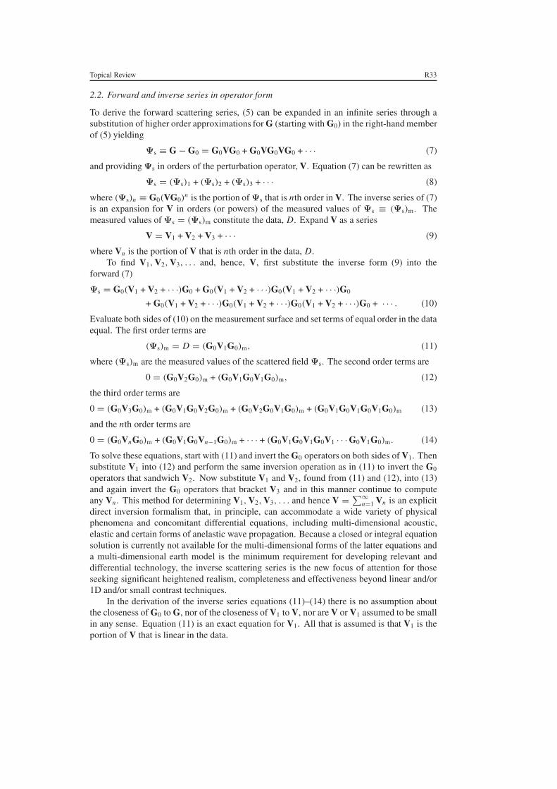
2.2. Forward and inverse series in operator form
To derive the forward scattering series, (5) can be expanded in an infinite series through asubstitution of higher order approximations for G (starting with G0) in the right-hand memberof (5) yielding
Ψs ≡ G − G0 = G0VG0 + G0VG0VG0 + · · · (7)
and providing Ψs in orders of the perturbation operator, V. Equation (7) can be rewritten as
Ψs = (Ψs)1 + (Ψs)2 + (Ψs)3 + · · · (8)
where (Ψs)n ≡ G0(VG0)n is the portion of Ψs that is nth order in V. The inverse series of (7)
is an expansion for V in orders (or powers) of the measured values of Ψs ≡ (Ψs)m. Themeasured values of Ψs = (Ψs)m constitute the data, D. Expand V as a series
V = V1 + V2 + V3 + · · · (9)
where Vn is the portion of V that is nth order in the data, D.To find V1, V2, V3, . . . and, hence, V, first substitute the inverse form (9) into the
forward (7)
Ψs = G0(V1 + V2 + · · ·)G0 + G0(V1 + V2 + · · ·)G0(V1 + V2 + · · ·)G0
+ G0(V1 + V2 + · · ·)G0(V1 + V2 + · · ·)G0(V1 + V2 + · · ·)G0 + · · · . (10)
Evaluate both sides of (10) on the measurement surface and set terms of equal order in the dataequal. The first order terms are
(Ψs)m = D = (G0V1G0)m, (11)
where (Ψs)m are the measured values of the scattered field Ψs. The second order terms are
0 = (G0V2G0)m + (G0V1G0V1G0)m, (12)
the third order terms are
0 = (G0V3G0)m + (G0V1G0V2G0)m + (G0V2G0V1G0)m + (G0V1G0V1G0V1G0)m (13)
and the nth order terms are
0 = (G0VnG0)m + (G0V1G0Vn−1G0)m + · · · + (G0V1G0V1G0V1 · · · G0V1G0)m. (14)
To solve these equations, start with (11) and invert the G0 operators on both sides of V1. Thensubstitute V1 into (12) and perform the same inversion operation as in (11) to invert the G0
operators that sandwich V2. Now substitute V1 and V2, found from (11) and (12), into (13)and again invert the G0 operators that bracket V3 and in this manner continue to computeany Vn . This method for determining V1, V2, V3, . . . and hence V = ∑∞
n=1 Vn is an explicitdirect inversion formalism that, in principle, can accommodate a wide variety of physicalphenomena and concomitant differential equations, including multi-dimensional acoustic,elastic and certain forms of anelastic wave propagation. Because a closed or integral equationsolution is currently not available for the multi-dimensional forms of the latter equations anda multi-dimensional earth model is the minimum requirement for developing relevant anddifferential technology, the inverse scattering series is the new focus of attention for thoseseeking significant heightened realism, completeness and effectiveness beyond linear and/or1D and/or small contrast techniques.
In the derivation of the inverse series equations (11)–(14) there is no assumption aboutthe closeness of G0 to G, nor of the closeness of V1 to V, nor are V or V1 assumed to be smallin any sense. Equation (11) is an exact equation for V1. All that is assumed is that V1 is theportion of V that is linear in the data.
R34 Topical Review
If one were to assume that V1 is close to V and then treat (11) as an approximate solutionfor V, that would then correspond to the inverse Born approximation. In the formalism ofthe inverse scattering series, the assumption of V ≈ V1 is never made. The inverse Bornapproximation inputs the data D and G0 and outputs V1 which is then treated as an approximateV. The forward Born approximation assumes that, in some sense, V is small and the inverseBorn assumes that the data, (Ψs)m, are small. The forward and inverse Born approximationsare two separate and distinct methods with different inputs and objectives. The forward Bornapproximation for the scattered field, Ψs, uses a linear truncation of (7) to estimate Ψs:
Ψs∼= G0VG0
and inputs G0 and V to find an approximation to Ψs. The inverse Born approximation inputsD and G0 and solves for V1 as the approximation to V by inverting
(Ψs)m = D ∼= (G0VG0)m.
All of current seismic processing methods for imaging and inversion are differentincarnations of using (11) to find an approximation for V [3], where G0 ≈ G, and thatfact explains the continuous and serious effort in seismic and other applications to build evermore realism and completeness into the reference differential operator, L0, and its impulseresponse, G0. As with all technical approaches, the latter road (and current mainstreamseismic thinking) eventually leads to a stage of maturity where further allocation of researchand technical resource will no longer bring commensurate added value or benefit. The inverseseries methods provide an opportunity to achieve objectives in a direct and purposeful mannerwell beyond the reach of linear methods for any given level of a priori information.
2.3. The inverse series is not iterative linear inversion
The inverse scattering series is a procedure that is separate and distinct from iterative linearinversion. Iterative linear inversion starts with (11) and solves for V1. Then a new referenceoperator, L′
0 = L0+V1, impulse response, G ′0 (where L′
0G ′0 = −δ), and data, D′ = (G−G ′
0)m,are input to a new linear inverse form
D′ = (G′0V′
1G′0)m
where a new operator, G′0, has to then be inverted from both sides of V′
1. These linear steps areiterated and at each step a new, and in general more complicated, operator (or matrix, Frechetderivative or sensitivity matrix) must be inverted. In contrast, the inverse scattering seriesequations (11)–(14) invert the same original input operator, G0, at each step.
2.4. Development of the inverse series for seismic processing
The inverse scattering series methods were first developed by Moses [10], Prosser [11] andRazavy [12] and were transformed for application to a multi-dimensional earth and explorationseismic reflection data by Weglein et al [4] and Stolt and Jacobs [13]. The first question inconsidering a series solution is the issue of convergence followed closely by the question ofrate of convergence. The important pioneering work on convergence criteria for the inverseseries by Prosser [11] provides a condition which is difficult to translate into a statement onthe size and duration of the contrast between actual and reference media. Faced with that lackof theoretical guidance, empirical tests of the inverse series were performed by Carvalho [14]for a 1D acoustic medium. Test results indicated that starting with no a priori information,convergence was observed but appeared to be restricted to small contrasts and duration ofthe perturbation. Convergence was only observed when the difference between actual earth

Topical Review R35
acoustic velocity and water (reference) velocity was less than approximately 11%. Since, formarine exploration, the acoustic wave speed in the earth is generally larger than 11% of theacoustic wave speed in water (1500 m s−1), the practical value of the entire series without apriori information appeared to be quite limited.
A reasonable response might seem to be to use seismic methods that estimate the velocitytrend of the earth to try to get the reference medium proximal to the actual and that in turncould allow the series to possibly converge. The problem with that line of reasoning was thatvelocity trend estimation methods assumed that multiples were removed prior to that analysis.Furthermore, concurrent with these technical deliberations and strategic decisions (around1989–90) was the unmistakably consistent and clear message heard from petroleum industryoperating units that inadequate multiple removal was an increasingly prioritized and seriousimpediment to their success.
Methods for removing multiples at that time assumed either one or more of the following:(1) the earth was 1D, (2) the velocity model was known, (3) the reflectors generating themultiples could be defined, (4) different patterns could be identified in waves from primaries andmultiples or (5) primaries were random and multiples were periodic. All of these assumptionswere seriously violated in deep water and/or complex geology and the methods based uponthem often failed to perform, or produced erroneous or misleading results.
The interest in multiples at that time was driven in large part by the oil industry trend toexplore in deep water (>1 km) where the depth alone can cause multiple removal methods basedon periodicity to seriously violate their assumptions. Targets associated with complex multi-dimensional heterogeneous and difficult to estimate geologic conditions presented challengesfor multiple removal methods that rely on having 1D assumptions or knowledge of inaccessibledetails about the reflectors that were the source of these multiples.
The inverse scattering series is the only multi-dimensional direct inversion formalism thatcan accommodate arbitrary heterogeneity directly in terms of the reference medium, throughG0, i.e., with estimated rather than actual propagation,G. The confluence of these factors led tothe development of thinking that viewed inversion as a series of tasks or stages and to viewingmultiple removal as a step within an inversion machine which could perhaps be identified,isolated and examined for its convergence properties and demands on a priori information anddata.
2.5. Subseries of the inverse series
A combination of factors led to imagining inversion in terms of steps or stages with intermediateobjectives towards the ultimate goal of identifying earth material properties. These factors are:
(1) the inverse series represents the only multi-dimensional direct seismic inversion methodthat performs its mathematical operations directly in terms of a single, fixed, unchangingand assumed to be inadequate G0, i.e., which is assumed not to be equal to the adequatepropagator, G;
(2) numerical tests that suggested an apparent lack of robust convergence of the overall series(when starting with no a priori information);
(3) seismic methods that are used to determine a priori reference medium information, e.g.,reference propagation velocity, assume the data consist of primaries and hence were (andare) impeded by the presence of multiples;
(4) the interest in extracting something of value from the only formalism for complete directmulti-dimensional inversion; and
(5) the clear and unmistakeable industry need for more effective methods that removemultiples especially in deep water and/or from data collected over an unknown, complex,ill-defined and heterogeneous earth.
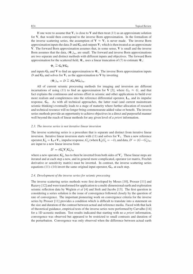
R36 Topical Review
Each stage in inversion was defined as achieving a task or objective: (1) removing free-surface multiples; (2) removing internal multiples; (3) locating and imaging reflectors in space;and (4) determining the changes in earth material properties across those reflectors. The ideawas to identify, within the overall series, specific distinct subseries that performed these focusedtasks and to evaluate these subseries for convergence, requirements for a priori information, rateof convergence, data requirements and theoretical and practical prerequisites. It was imagined(and hoped) that perhaps a subseries for one specific task would have a more favourable attitudetowards, e.g., convergence in comparison to the entire series. These tasks, if achievable, wouldbring practical benefit on their own and, since they are contained within the construction ofV1, V2, . . . in (12)–(14), each task would be realized from the inverse scattering series directlyin terms of the data, D, and reference wave propagation, G0.
At the outset, many important issues regarding this new task separation strategy were open(and some remain open). Among them were
(1) Does the series in fact uncouple in terms of tasks?(2) If it does uncouple, then how do you identify those uncoupled task-specific subseries?(3) Does the inverse series view multiples as noise to be removed, or as signal to be used for
helping to image/invert the target?(4) Do the subseries derived for individual tasks require different algorithms for different
earth model types (e.g., acoustic version and elastic version)?(5) How can you know or determine, in a given application, how many terms in a subseries
will be required to achieve a certain degree of effectiveness?
We will address and respond to these questions in this article and list others that are outstandingor the subject of current investigation.
How do you identify a task-specific subseries? The pursuit of task-specific subseriesused several different types of analysis with testing of new concepts to evaluate, refine anddevelop embryonic thinking largely based on analogues and physical intuition. To begin, theforward and inverse series, (7) and (11)–(14), have a tremendous symmetry. The forwardseries produces the scattered wavefield, Ψs, from a sum of terms each of which is composedof the operator, G0, acting on V. When evaluated on the measurement surface, the forwardseries creates all of the data, (Ψs)m = D, and contains all recorded primaries and multiples.The inverse series produces V from a series of terms each of which can be interpreted as theoperator G0 acting on the recorded data, D. Hence, in scattering theory the same operator G0
as acts on V to create data acts on D to invert data. If we consider
(G0VG0)m = (G0(V1 + V2 + V3 + · · ·)G0)m
and use (12)–(14), we find
(G0VG0)m = (G0V1G0)m − (G0V1G0V1G0)m + · · · . (15)
There is a remarkable symmetry between the inverse series (15) and the forward series (7)evaluated on the measurement surface:
(Ψs)m = (G0VG0)m + (G0VG0VG0)m + · · · . (16)
In terms of diagrams, the inverse series for V, (15) can be represented as
Topical Review R37
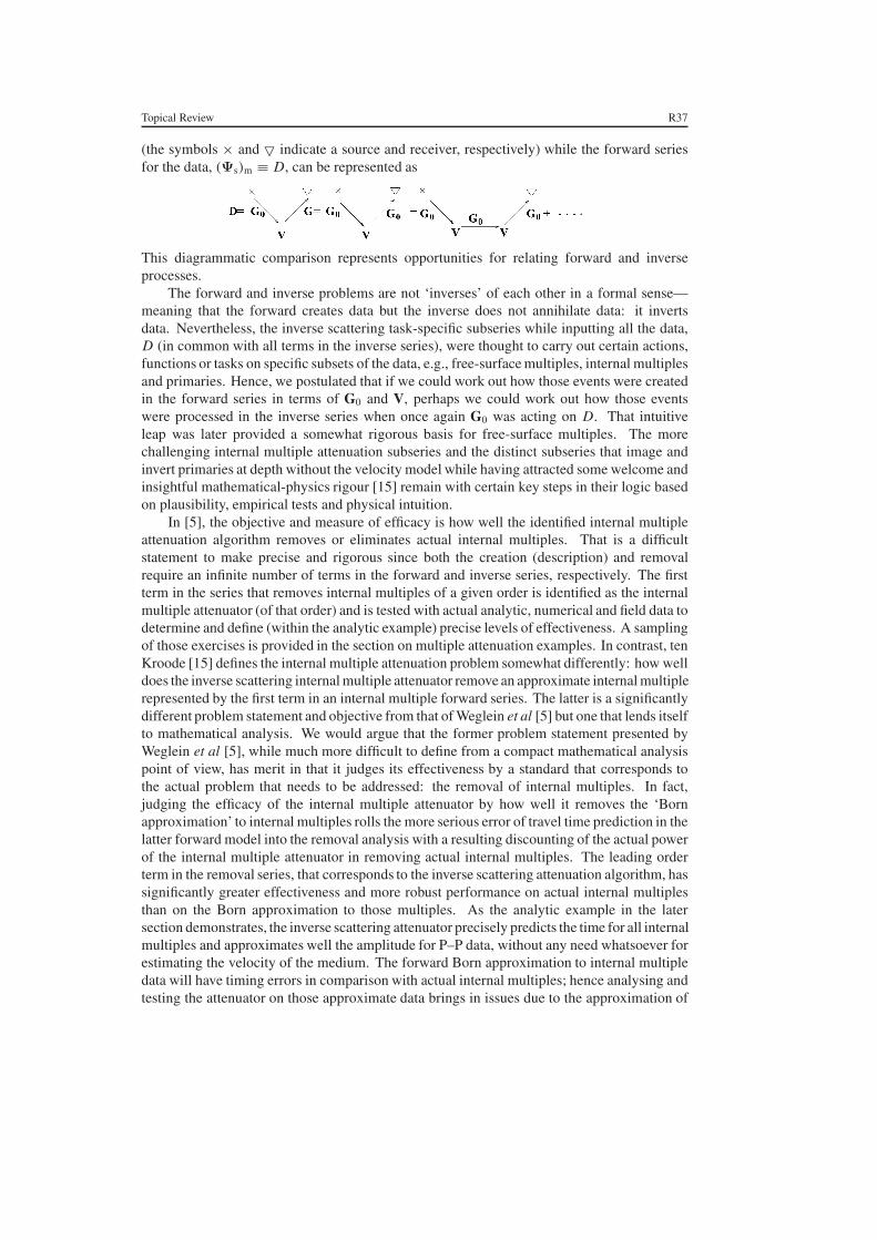
(the symbols × and � indicate a source and receiver, respectively) while the forward seriesfor the data, (Ψs)m ≡ D, can be represented as
This diagrammatic comparison represents opportunities for relating forward and inverseprocesses.
The forward and inverse problems are not ‘inverses’ of each other in a formal sense—meaning that the forward creates data but the inverse does not annihilate data: it invertsdata. Nevertheless, the inverse scattering task-specific subseries while inputting all the data,D (in common with all terms in the inverse series), were thought to carry out certain actions,functions or tasks on specific subsets of the data, e.g., free-surface multiples, internal multiplesand primaries. Hence, we postulated that if we could work out how those events were createdin the forward series in terms of G0 and V, perhaps we could work out how those eventswere processed in the inverse series when once again G0 was acting on D. That intuitiveleap was later provided a somewhat rigorous basis for free-surface multiples. The morechallenging internal multiple attenuation subseries and the distinct subseries that image andinvert primaries at depth without the velocity model while having attracted some welcome andinsightful mathematical-physics rigour [15] remain with certain key steps in their logic basedon plausibility, empirical tests and physical intuition.
In [5], the objective and measure of efficacy is how well the identified internal multipleattenuation algorithm removes or eliminates actual internal multiples. That is a difficultstatement to make precise and rigorous since both the creation (description) and removalrequire an infinite number of terms in the forward and inverse series, respectively. The firstterm in the series that removes internal multiples of a given order is identified as the internalmultiple attenuator (of that order) and is tested with actual analytic, numerical and field data todetermine and define (within the analytic example) precise levels of effectiveness. A samplingof those exercises is provided in the section on multiple attenuation examples. In contrast, tenKroode [15] defines the internal multiple attenuation problem somewhat differently: how welldoes the inverse scattering internal multiple attenuator remove an approximate internal multiplerepresented by the first term in an internal multiple forward series. The latter is a significantlydifferent problem statement and objective from that of Weglein et al [5] but one that lends itselfto mathematical analysis. We would argue that the former problem statement presented byWeglein et al [5], while much more difficult to define from a compact mathematical analysispoint of view, has merit in that it judges its effectiveness by a standard that corresponds tothe actual problem that needs to be addressed: the removal of internal multiples. In fact,judging the efficacy of the internal multiple attenuator by how well it removes the ‘Bornapproximation’ to internal multiples rolls the more serious error of travel time prediction in thelatter forward model into the removal analysis with a resulting discounting of the actual powerof the internal multiple attenuator in removing actual internal multiples. The leading orderterm in the removal series, that corresponds to the inverse scattering attenuation algorithm, hassignificantly greater effectiveness and more robust performance on actual internal multiplesthan on the Born approximation to those multiples. As the analytic example in the latersection demonstrates, the inverse scattering attenuator precisely predicts the time for all internalmultiples and approximates well the amplitude for P–P data, without any need whatsoever forestimating the velocity of the medium. The forward Born approximation to internal multipledata will have timing errors in comparison with actual internal multiples; hence analysing andtesting the attenuator on those approximate data brings in issues due to the approximation of

R38 Topical Review
Figure 3. The marine configuration and reference Green function.
the forward data in the test that are misattributed to the properties of the attenuator. Tests suchas those presented in [16, 17] and in the latter sections of this article are both more realisticand positive for the properties of the attenuator when tested and evaluated on real, in contrastto approximate, internal multiples.
In fact, for internal multiples, understanding how the forward scattering series produces anevent only hints at where the inverse process might be located. That ‘hint’, due to a symmetrybetween event creation and event processing for inversion, turned out to be a suggestion,with an infinite number of possible realizations. Intuition, testing and subtle refinement ofconcepts ultimately pointed to where the inverse process was located. Once the location wasidentified, further rationalizations could be provided, in hindsight, to explain the choice amongthe plethora of possibilities. Intuition has played an important role in this work,which is neitheran apology nor an expression of hubris, but a normal and expected stage in the developmentand evolution of fundamentally new concepts. This specific issue is further discussed in thesection on internal multiples.
3. Marine seismic exploration
In marine seismic exploration sources and receivers are located in the water column. Thesimplest reference medium that describes the marine seismic acquisition geometry is a half-space of water bounded by a free surface at the air–water interface. The reference Greenoperator, G0, consists of two parts:
G0 = Gd0 + GFS
0 , (17)
where Gd0 is the direct propagating, causal, whole-space Green operator in water and GFS
0 isthe additional part of the Green operator due to the presence of the free surface (see figure 3).GFS
0 corresponds to a reflection off the free surface.In the absence of a free surface, the reference medium is a whole space of water and Gd
0 isthe reference Green operator. In this case, the forward series equation (7) describing the data isconstructed from the direct propagating Green operator, Gd
0, and the perturbation operator, V.With our choice of reference medium, the perturbation operator characterizes the differencebetween earth properties and water; hence, the support of V begins at the water bottom. Withthe free surface present, the forward series is constructed from G0 = Gd
0 + GFS0 and the same
perturbation operator, V. Hence, GFS0 is the sole difference between the forward series with and
without the free surface; therefore GFS0 is responsible for generating those events that owe their
existence to the presence of the free surface, i.e., ghosts and free-surface multiples. Ghosts areevents that either start their history propagating up from the source and reflecting down fromthe free surface or end their history as the downgoing portion of the recorded wavefield at thereceiver, having its last downward reflection at the free surface (see figure 4).

Topical Review R39
Figure 4. Examples of ghost events: (a) source ghost, (b) receiver ghost and (c) source–receiverghost.
In the inverse series, equations (11)–(14), it is reasonable to infer that GFS0 will be
responsible for all the extra tasks that inversion needs to perform when starting with datacontaining ghosts and free-surface multiples rather than data without those events. Thoseextra inverse tasks include deghosting and the removal of free-surface multiples. In the sectionon the free-surface demultiple subseries that follows, we describe how the extra portion of thereference Green operator due to the free surface, GFS
0 , performs deghosting and free-surfacemultiple removal.
Once the events associated with the free surface are removed, the remaining measuredfield consists of primaries and internal multiples. For a marine experiment in the absence of afree surface, the scattered field, Ψ′
s, can be expressed as a series in terms of a reference mediumconsisting of a whole space of water, the reference Green operator, Gd
0, and the perturbation,V, as follows:
Ψ′s = Gd
0VGd0 + Gd
0VGd0VGd
0 + Gd0VGd
0VGd0VGd
0 + · · ·= (Ψ′
s)1 + (Ψ′s)2 + (Ψ′
s)3 + · · · . (18)
The values of Ψ′s on the measurement surface, D′, are the data, D, collected in the absence of
a free surface; i.e., D′ consists of primaries and internal multiples:
D′ = D′1 + D′
2 + D′3 + · · · . (19)
D′ is the data D without free-surface events. Unfortunately, the free-space Green function,Gd
0, does not separate into a part responsible for primaries and a part responsible for internalmultiples. As a result, a totally new concept was required and introduced to separate the tasksassociated with Gd
0 [5].The forward scattering series (18) evaluated on the measurement surface describes data
and every event in those data in terms of a series. Each term of the series corresponds to asequence of reference medium propagations, Gd
0, and scatterings off the perturbation, V. Aseismic event represents the measured arrival of energy that has experienced a specific set ofactual reflections, R, and transmissions, T , at reflectors and propagations, p, governed bymedium properties between reflectors. A complete description of an event would typicallyconsist of a single term expression with all the actual episodes of R, T and p in its history. Theclassification of an event in D′ as a primary or as an internal multiple depends on the numberand type of actual reflections that it has experienced. The scattering theory description of anyspecific event in D′ requires an infinite series necessary to build the actual R, T and p factorsin terms of reference propagation, Gd
0, and the perturbation operator, V. That is, R, T andp are non-linearly related to Gd
0 and V. Even the simplest water bottom primary for whichG0 = Gd
0 requires a series for its description in scattering theory (to produce the water bottomreflection, R, from an infinite series, non-linear in V ). We will illustrate this concept witha simple example later in this section. Hence, two chasms need to be bridged to determinethe subseries that removes internal multiples. The first requires a map between primary andinternal multiples in D′ and their description in the language of forward scattering theory,

R40 Topical Review
Figure 5. The 1D plane-wave normal incidence acoustic example.
Gd0 and V; the second requires a map between the construction of internal multiple events in
the forward series and the removal of these events in the inverse series.The internal multiple attenuation concept requires the construction of these two
dictionaries: one relates seismic events to a forward scattering description, the second relatesforward construction to inverse removal. The task separation strategy requires that those twomaps be determined. Both of these multi-dimensional maps were originally inferred usingarguments of physical intuition and mathematical reasonableness. Subsequently, Matson [18]provided a mathematically rigorous map of the relationship between seismic events and theforward scattering series for 1D constant density acoustic media that confirm the originalintuitive arguments. Recent work by Nita et al [19] and Innanen and Weglein [20] extendsthat work to prestack analysis and absorptive media, respectively. The second map, relatingforward construction and inverse removal, remains largely based on its original foundation.Recently, ten Kroode [15] presented a formal mathematical analysis for certain aspects of aforward to inverse internal multiple map (discussed in the previous section) based on a leadingorder definition of internal multiples and assumptions about the symmetry involved in thelatter map. For the purpose of this article, we present only the key logical steps of the originalarguments that lead to the required maps. The argument of the first map is presented here;the second map, relating forward construction and inverse removal, is presented in the nextsection.
To understand how the forward scattering series describes a particular event, it is usefulto recall that the forward series for D′ is a generalized Taylor series in the scattering operator,V [21]. But what is the forward scattering subseries for a given event in D′? Since a specificevent consists of a set of actual R, T and p factors, it is reasonable to start by asking how theseindividual factors are expressed in terms of the perturbation operator. Consider the simpleexample of one dimensional acoustic medium consisting of a single interface and a normalincidence plane wave, eikz , illustrated in figure 5.
Let the reference medium be a whole space with acoustic velocity, c0. The actual andreference differential equations describing the actual and reference wavefields, P and P0, are[
d2
dz2+
ω2
c2(z)
]P(z, ω) = 0
and [d2
dz2+
ω2
c20
]P0(z, ω) = 0,
where c(z) is the actual velocity.The perturbation operator, V, is
V = L − L0 = ω2
c2(z)− ω2
c20
.

R42 Topical Review
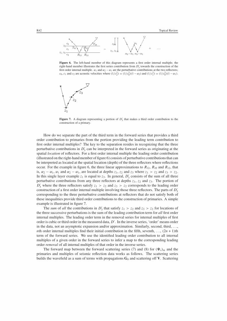
Figure 6. The left-hand member of this diagram represents a first order internal multiple; theright-hand member illustrates the first series contribution from D′
3 towards the construction of thefirst order internal multiple. α1 and α2 − α1 are the perturbative contributions at the two reflectors;c0, c1 and c2 are acoustic velocities where (1/c2
2) = (1/c20)(1 − α2) and (1/c2
1) = (1/c20)(1 − α1).
Figure 7. A diagram representing a portion of D′3 that makes a third order contribution to the
construction of a primary.
How do we separate the part of the third term in the forward series that provides a thirdorder contribution to primaries from the portion providing the leading term contribution tofirst order internal multiples? The key to the separation resides in recognizing that the threeperturbative contributions in D′
3 can be interpreted in the forward series as originating at thespatial location of reflectors. For a first order internal multiple the leading order contribution(illustrated on the right-hand member of figure 6) consists of perturbative contributions that canbe interpreted as located at the spatial location (depth) of the three reflectors where reflectionsoccur. For the example in figure 6, the three linear approximations to R12, R10 and R12, thatis, α2 − α1, α1 and α2 − α1, are located at depths z1, z2 and z3 where z1 > z2 and z3 > z2.In this single layer example z1 is equal to z3. In general, D′
3 consists of the sum of all threeperturbative contributions from any three reflectors at depths z1, z2 and z3. The portion ofD′
3 where the three reflectors satisfy z1 > z2 and z3 > z2 corresponds to the leading orderconstruction of a first order internal multiple involving those three reflectors. The parts of D′
3corresponding to the three perturbative contributions at reflectors that do not satisfy both ofthese inequalities provide third order contributions to the construction of primaries. A simpleexample is illustrated in figure 7.
The sum of all the contributions in D′3 that satisfy z1 > z2 and z3 > z2 for locations of
the three successive perturbations is the sum of the leading contribution term for all first orderinternal multiples. The leading order term in the removal series for internal multiples of firstorder is cubic or third order in the measured data, D′. In the inverse series, ‘order’ means orderin the data, not an asymptotic expansion and/or approximation. Similarly, second, third, . . .,nth order internal multiples find their initial contribution in the fifth, seventh, . . ., (2n + 1)thterm of the forward series. We use the identified leading order contribution to all internalmultiples of a given order in the forward series to infer a map to the corresponding leadingorder removal of all internal multiples of that order in the inverse series.
The forward map between the forward scattering series (7) and (8) for (Ψs)m and theprimaries and multiples of seismic reflection data works as follows. The scattering seriesbuilds the wavefield as a sum of terms with propagations G0 and scattering off V. Scattering

Topical Review R43
Figure 8. A s cattering series description of primaries and internal multiples: P1—primary with onereflection; P2—primary with one reflection and onetransmission; P3—primary with one reflectionand a self-interaction; M1—first order internal multiple (one downward reflection); M2—secondorder internal multiple (two downward reflections).occurs in all directions from the scattering pointVand the relative amplitude in a givendirection is determined by the isotropy (or anisotropy) of the scattering operator. A scatteringoperator being anisotropic is distinct from physical anisotropy; the latter means that the wavespeed in theactual medium at a point is a function of the direction of propagation of thewave at that point. A two parameter, variable velocityand density, acoustic isotropic mediumhas a n a nisotropic scattering operator (see (6)). In any case, since primaries and multiplesare defined in terms of reflections, we propose that primaries and internal multiples will bedistinguished by the number of reflection-like scatterings in their forward description, figure 8.A refl ection-like scattering occurs when the incident wave moves away from the measurementsurface towards the scattering point and the wave emerging from the scattering point movestowards the measurement surface.Every reflection event in seismic data requires contributions from an infinite number ofterms in the scattering theorydescription. Even with water velocity as the reference, and forevents where the actual propagation medium is water, then the simplest primaries, i.e., thewater bottom reflection, require an infinitenumber of contributions to takeG0andVintoG0andR,whereVandRcorrespond to the perturbation operator and reflection coefficient at thewater bottom, respectively. For a primary originating below the water bottom, the series hastodeal with issues beyond turning the local value ofVinto the local reflection coefficient,R.In the latter case, the reference Green function,G0,nolonger corresponds to the propagationdown to and back from the reflector (G=G0)and the terms in the series beyond the firstare required to correct for timing errors and ignored transmission coefficients, in addition totakingVintoR.The remarkable fact is that all primaries are constructed in the forward series by portionsof every term in the series. The contributing part has one and only one upward reflection-like scattering. Furthermore, internal multiples of a given order have contributions from allterms that have exactly a number of downward reflection-like scatterings corresponding to theorderofthatinternal multiple. The order of the internal multiple is defined by the number ofdownward reflections, independent of the location of the reflectors (see figure 8).

R44 Topical Review
Figure 9. Maps for inverse scattering subseries. Map I takes seismic events to a scattering seriesdescription: D(t) = (Ψs)m consists of primaries and multiples; (Ψs)m = D(t) represents aforward series in terms of G0 and V. Map II takes forward construction of events to inverseprocessing of those events: (G0VG0)m = (G0V1G0)m − (G0V1G0V1G0)m + · · ·.
All internal multiples of first order begin their creation in the scattering series in the portionof the third term of (Ψs)m with three reflection-like scatterings. All terms in the fourth andhigher terms of (Ψs)m that consist of three and only three reflection-like scatterings plus anynumber of transmission-like scatterings (e.g., event (b) in figure 8) and/or self-interactions(e.g., event (c) in figure 8) also contribute to the construction of first order internal multiples.
Further research in the scattering theory descriptions of seismic events is warrantedand under way and will strengthen the first of the two key logic links (maps) required fordevelopments of more effective and better understood task-specific inversion procedures.
4. The inverse series and task separation: terms with coupled and uncoupled tasks
As discussed in section 3, GFS0 is the agent in the forward series that creates all events that come
into existence due to the presence of the free surface (i.e., ghosts and free-surface multiples);when the inverse series starts with data that include free-surface-related events and, theninversion has additional tasks to perform on the way to constructing the perturbation, V (i.e.,deghosting and free-surface multiple removal); and, for the marine case, the forward andinverse reference Green operator, G0, consists of Gd
0 plus GFS0 . These three arguments taken
together imply that, in the inverse series, GFS0 is the ‘removal operator’ for the surface-related
events that it created in the forward series.With that thought in mind, we will describe the deghosting and free-surface multiple
removal subseries. The inverse series expansions, equations (11)–(14), consist of terms(G0VnG0)m with G0 = Gd
0 + GFS0 . Deghosting is realized by removing the two outside
G0 = Gd0 + GFS
0 functions and replacing them with Gd0. The Green function Gd
0 represents adowngoing wave from source to V and an upgoing wave from V to the receiver (details areprovided in section 5.4).
The source and receiver deghosted data, D, are represented by D = (Gd0V1Gd
0)m. After thedeghosting operation, the objective is to remove the free-surface multiples from the deghosteddata, D.
The terms in the inverse series expansions, (11)–(14), replacing D with input D, containboth Gd
0 and GFS0 between the operators Vi . The outside Gd
0 s only indicate that the data havebeen source and receiver deghosted. The inner Gd
0 and GFS0 are where the four inversion tasks
reside. If we consider the inverse scattering series and G0 = Gd0 + GFS
0 and if we assumethat the data have been source and receiver deghosted (i.e., Gd
0 replaces GFS0 on the outside
contributions), then the terms in the series are of three types:
Type 1: (Gd0Vi GFS
0 V j GFS0 VkGd
0)m
Type 2: (Gd0Vi GFS
0 V j Gd0VkGd
0)m
Type 3: (Gd0Vi Gd
0V j Gd0VkGd
0)m.
Topical Review R45
We interpret these types of term from a task isolation point of view. Type 1 terms have onlyGFS
0 between two Vi , V j contributions; these terms when added to D remove free-surfacemultiples and perform no other task. Type 2 terms have both Gd
0 and GFS0 between two Vi , V j
contributions; these terms perform free-surface multiple removal plus a task associated withGd
0. Type 3 have only Gd0 between two Vi , V j contributions; these terms do not remove any
free-surface multiples.The idea behind task separated subseries is twofold:
(1) isolate the terms in the overall series that perform a given task as if no other tasks exist(e.g., type 1 above) and
(2) do not return to the original inverse series with its coupled tasks involving GFS0 and Gd
0,but rather restart the problem with input data free of free-surface multiples, D′.
Collecting all type 1 terms we have
D′1 ≡ D = (Gd
0V1Gd0)m (11′)
D′2 = −(Gd
0V1GFS0 V1Gd
0)m (12′)D′
3 = −(Gd0V1GFS
0 V1GFS0 V1Gd
0)m
− (Gd0V1GFS
0 V2Gd0)m
− (Gd0V1GFS
0 V2Gd0)m (13′)
....
D′3 can be simplified as
D′3 = +(Gd
0V1GFS0 V1GFS
0 V1Gd0)m
(this reduction of (13′) is not valid for type 2 or type 3 terms). D′ = ∑∞i=1 D′
i are thedeghosted and free-surface demultipled data. The new free-surface demultipled data, D′,consist of primaries and internal multiples and an inverse series for V = ∑∞
i=1V′i where V′
iis the portion of V that is i th order in primaries and internal multiples. Collecting all type 3terms:
D′ = (Gd0V′
1Gd0)m (11′′)
(Gd0V ′
2Gd0)m = −(Gd
0V′1Gd
0V′1Gd
0)m (12′′)(Gd
0V ′3Gd
0)m = −(Gd0V′
1Gd0V′
1Gd0V′
1Gd0)m
− (Gd0V′
1Gd0V ′
2Gd0)m
− (Gd0V′
2Gd0V′
1Gd0)m (13′′)
....
When the free surface is absent, Gd0 creates primaries and internal multiples in the forward
series and is responsible for carrying out all inverse tasks on those same events in the inverseseries.
We repeat this process seeking to isolate terms that only ‘care about’ the responsibilityof Gd
0 towards removing internal multiples. No coupled task terms that involve bothinternal multiples and primaries are included. After the internal multiples attenuation taskis accomplished we restart the problem once again and write an inverse series whose inputconsists only of primaries. This task isolation and restarting of the definition of the inversion
R46 Topical Review
procedure strategy have several advantages over staying with the original series. Thoseadvantages include the recognition that a task that has already been accomplished is a form ofnew information and makes the subsequent and progressively more difficult tasks in our listconsiderably less daunting compared to the original all-inclusive data series approach. Forexample, after removing multiples with a reference medium of water speed, it is easier toestimate a variable background to aid convergence for subsequent tasks whose subseries mightbenefit from that advantage. Note that the V represents the difference between water and earthproperties and can be expressed as V = ∑∞
i=1 Vi and V = ∑∞i=1 V′
i . However, Vi = V′i since
Vi assumes that the data are D (primaries and all multiples) and V′i assumes that the data are
D′ (primaries and only internal multiples). In other words, V1 is linear in all primaries andfree-surface and internal multiples, while V′
1 is linear in all primaries and internal multiplesonly.
5. An analysis of the earth model type and the inverse series and subseries
5.1. Model type and the inverse series
To invert for medium properties requires choosing a set of parameters that you seek to identify.The chosen set of parameters (e.g., P and S wave velocity and density) defines an earth modeltype (e.g., acoustic, elastic, isotropic, anisotropic earth) and the details of the inverse serieswill depend on that choice. Choosing an earth model type defines the form of L, L0 and V. Onthe way towards identifying the earth properties (for a given model type), intermediate tasksare performed, such as the removal of free-surface and internal multiples and the location ofreflectors in space.
It will be shown below that the free-surface and internal multiple attenuation subseries notonly do not require subsurface information for a given model type, but are even independentof the earth model type itself for a very large class of models. The meaning of model type-independent task-specific subseries is that the defined task is achievable with precisely thesame algorithm for an entire class of earth model types. The members of the model typeclass that we are considering satisfy the convolution theorem and include acoustic, elastic andcertain anelastic media.
In this section, we provide a more general and complete formalism for the inverse series,and especially the subseries, than has appeared in the literature to date. That formalism allowsus to examine the issue of model type and inverse scattering objectives. When we discuss theimaging and inversion subseries in section 8, we use this general formalism as a frameworkfor defining and addressing the new challenges that we face in developing subseries thatperform imaging at depth without the velocity and inverting large contrast complex targets.All inverse methods for identifying medium properties require specification of the parameters tobe determined, i.e., of the assumed earth model type that has generated the scattered wavefield.To understand how the free-surface multiple removal and internal multiple attenuation task-specific subseries avoid this requirement (and to understand under what circumstances theimaging subseries would avoid that requirement as well), it is instructive to examine themathematical physics and logic behind the classic inverse series and see precisely the role thatmodel type plays in the derivation.
References for the inverse series include [4, 10, 12, 13]. The inverse series paper byRazavy [12] is a lucid and important paper relevant to seismic exploration. In that paper, Razavyconsiders a normal plane wave incident on a one dimensional acoustic medium. We followRazavy’s development to see precisely how model type enters and to glean further physicalinsight from the mathematical procedure. Then we introduce a perturbation operator, V,

Topical Review R47
F i g ure10.T h e s catteringexperiment:aplanewave i ncidentupontheperturbation,α . g e n e r a l e n o u g h i n s t r u c t u r e t o a c c o m m o d a t e t h e e n t i r e c l a s s o f e a r t h m o d e l t y p e s u n d e r
c o n s i d e r a t i o n . Fin a l l y , i f a p r o c e s s ( i . e . , a s u b s e r i e s ) c a n b e p e r f o r m e d w i t h o u t s p e c i f y i n g h o wV d e p e n d s o n t h e e a r t h p r o p e r t y c h a n g e s ( i . e . , w h a t s e t o f e a r t h p r o p e r t i e s a r e a s s u m e d t o v a r y i n s i d eV ) , thentheprocessitselfisindep e n d e n t o f e a r t h m o d e l t y p e . 3 7 2 . I n v e r s e s e r i e s f o r a 1 D a c o u s t i c c o n s t a n t d e n s i t y m e d i u m Startwiththe1Dvariablevelocity,constan t d e n s i t y a c o u s t i c w a v e e q u a t i o n , w h e r ec ( z ) isthewavespe e d a n d � ( z , t )isapressurefieldatlocationz a t t i m e t . T h e e q u a t i o n t h a t � ( z , t ) satisfiesis( ∂ 2
∂ z 2 − 1c 2 ( z ) ∂ 2∂ t 2 )
� ( z , t ) = 0 ( 2 0 ) a n d a f t e r a t e m p o r a l F o u r i e r t r a n s f o r m ,t → ω ,
( d 2
d z 2 +
ω 2
c 2 ( z ) )
� ( z , ω ) = 0. ( 2 1 ) Chara c t e r i z e t h e v e l o c i t y c o n fi g u r a t i o n c ( z ) intermsofar e f e r e n c e v e l o c i t y , c 0 , a n d p e r t u r b a t i o n , α : 1
c 2 ( z )
= 1
c 2 0 ( 1 − α (z ) ) . ( 2 2 ) T h e e x p e r i m e n t c o n s i s t s o f a p l a n e w a v e e i k z w h e r ek = ω / c 0 inc i d e n t u p o n α (z ) f r o m t h e l e f t ( seefig u r e 1 0 ) . A s s u m e h e r e t h a tα h a s c o m p a c t s u p p o r t a n d t h a t t h e i n c i d e n t w a v e a p p r o a c h e sα f r o m t h e s a m e s i d e a s t h e s c a t t e r e d fi e l d i s m e a s u r e d . L e t b ( k) d e n o t e t h e o v e r a l l r e fl e c t i o n c o e f fi c i e n t f o r α (z ) . I t i s d e t e r m i n e d f r o m t h e r e fl e c t i o n d a t a a t a g i v e n f r e q u e n c y ω. T h e n e i k z a n d b ( k) e − i k z a r e t h e i n c i d e n t a n d t h e r e fl e c t e d wave s r e s p e c t i v e l y . R e w r i t e ( 2 1 ) a n d ( 2 2 ) a n d t h e i n c i d e n t w a v e b o u n d a r y c o n d i t i o n a s a n integrale q u a t i o n : � ( z , ω )= e i k z + 12 i k
∫ e i k | z − z ′ | k 2 α (z ′ ) � ( z ′ , ω ) dz ′ ( 2 3 ) a n d d e fi n e t h e s c a t t e r e d fi e l d� s : � s ( z , ω )≡ � (z , ω )− e i k z . Also,definethe T m a t r ix:
T ( p , k ) ≡
∫ e − i p z α (z ) � ( z ,k ) d z ( 2 4 )

R48 Topical Review
and the Fourier sandwich of the parameter, α:
α(p, k) ≡∫
e−ipzα(z)eikz dz.
The scattered field, �s, takes the form
�s(z, ω) = b(k)e−ikz (25)
for values of z less than the support of α(z). From (23) to (25) it follows that
T (−k, k)k
2i= b(k). (26)
Multiply (23) by α(z) and then Fourier transform over z to find
T (p, k) = α(p, k) − k2∫ ∞
−∞α(p, q)T (q, k)
q2 − k2 − iεdq (27)
where p is the Fourier conjugate of z and use has been made of the bilinear form of the Greenfunction. Razavy [12] also derives another integral equation by interchanging the roles ofunperturbed and perturbed operators, with L0 viewed as a perturbation of −V on a referenceoperator L:
α(p, k) = T (p, k) + k2∫ ∞
−∞T ∗(k, q)T (p, q)
q2 − k2 − iεdq. (28)
Finally, define W (k) as essentially the Fourier transform of the sought after perturbation, α:
W (k) ≡ α(−k, k) =∫ ∞
−∞e2ikzα(z) dz (29)
and recognize that predicting W (k) for all k produces α(z).From (28), we find, after setting p = −k,
W (k) = α(−k, k) = T (−k, k) + k2∫ ∞
−∞T ∗(k, q)T (−k, q)
q2 − k2 − iεdq. (30)
The left-hand member of (30) is the desired solution, W (k), but the right-hand member requiresboth T (−k, k) that we determine from 2ib(k)/k and T ∗(k, q)T (−k, q) for all q .
We cannot directly determine T (k, q) for all q from measurements outside α—onlyT (−k, k) from reflection data and T (k, k) from transmission data. If we could determineT (k, q) for all q , then (30) would represent a closed form solution to the (multi-dimensional)inverse problem. If T (−k, k) and T (k, k) relate to the reflection and transmission coefficients,respectively, then what does T (k, q) mean for all q?
Let us start with the integral form for the scattered field
�s(z, k) = 1
2π
∫ ∫eik′(z−z′)
k2 − k ′2 − iεdk ′ k2α(z′)�(z′, k) dz ′ (31)
and Fourier transform (31) going from the configuration space variable, z, to the wavenumber,p, to find
�s(p, k) =∫ ∫
δ(k ′ − p)e−ik′ z′
k2 − k ′2 − iεdk ′ k2α(z′)�(z′, k) dz′ (32)
and integrate over k ′ to find
�s(p, k) = k2
k2 − p2 − iε
∫e−ipz′
α(z′)�(z′, k) dz′. (33)

Topical Review R49
The integral in (33) is recognized from (24) as
�s(p, k) = k2 T (p, k)
k2 − p2 − iε. (34)
Therefore to determine T (p, k) for all p for any k is to determine �s(p, k) for all p and anyk (k = ω/c0). But to find �s(p, k) from �s(z, k) you need to compute∫ ∞
−∞e−ipz�s(z, k) dz, (35)
which means that it requires �s(z, k) at every z (not just at the measurement surface, i.e., afixed z value outside of α). Hence (30) would provide W (k) and therefore α(z), if we providenot only reflection data, b(k) = T (−k, k)2i/k, but also the scattered field, �s, at all depths, z.
Since knowledge of the scattered field, �s (and, hence, the total field), at all z could beused in (21) to directly compute c(z) at all z, there is not much point or value in treating (30)in its pristine form as a complete and direct inverse solution.
Moses [10] first presented a way around this dilemma. His thinking resulted in the inversescattering series and consisted of two necessary and sufficient ingredients: (1) model typecombined with (2) a solution for α(z) and all quantities that depend on α, order by order in thedata, b(k).
Expand α(z) as a series in orders of the measured data:
α = α1 + α2 + α3 + · · · =∞∑
n=1
αn (36)
where αn is nth order in the data D. When the inaccessible T (p, k), |p| = |k|, are ignored, (30)becomes the Born–Heitler approximation and a comparison to the inverse Born approximation(the Born approximation ignores the entire second term of the right-hand member of (30)) wasanalysed in [22].
It follows that all quantities that are power series (starting with power one) in α are alsopower series in the measured data:
T (p, k) = T1(p, k) + T2(p, k) + · · · , (37)
W (k) = W1(k) + W2(k) + · · · , (38)
α(p, k) = α1(p, k) + α2(p, k) + · · · . (39)
The model type (i.e., acoustic constant density variable velocity in the equation forpressure) provides a key relationship for the perturbation, V = k2α:
α(p, k) = W
(k − p
2
)(40)
that constrains the Fourier sandwich, α(p, k), to be a function of only the difference between kand p. This model type, combined with order by order analysis of the construction of T (p, k)
for p = k required by the series, provides precisely what we need to solve for α(z).Starting with the measured data, b(k), and substituting W = ∑
Wn , T = ∑Tn from (37)
and (38) into (30), we find∞∑
n=1
Wn(k) = 2i
kb(k) + k2
∫dq
q2 − k2 − iε
( ∞∑n=1
T ∗n
∞∑n=1
Tn
). (41)
To first order in the data, b(k), k > 0 (note that b∗(+k) = b(−k), k > 0), equation (41)provides
W1(k) = 2i
kb(k) (42)

R50 Topical Review
and (42) determines W1(k) for all k. From (42) together with (29) to first order in the data
W1(k) = α1(−k, k) =∫ ∞
−∞α1(z)e2ikz dz, (43)
we find α1(z). The next step towards our objective of constructing α(z) is to find α2(z).From W1(k) we can determine W1(k − p)/2 for all k and p and from (40) to first order in
the data
α1(p, k) = W1
(k − p
2
), (44)
which in turn provides α1(p, k) for all p, k. The relationship (44) is model type in action as seenby exploiting the acoustic model with variable velocity and the constant density assumption.
Next, (28) provides to first order α1(p, k) = T1(p, k) for all p and k. This is the criticallyimportant argument that builds the scattered field at all depths, order by order, in the measuredvalues of the scattered field. Substituting the α1, T1 relationship into (30), we find the secondorder relationship in the data:
W2(k) = k2∫ ∞
−∞dq
q2 − k2 − iεT ∗
1 (k, q)T1(−k, q) (45)
and
W2(k) =∫ ∞
−∞e2ikzα2(z) dz. (46)
After finding α2(z) we can repeat the steps to determine the total α order by order:
α = α1(z) + α2(z) + · · · .Order by order arguments and the model type allow
T1(p, k) = α1(p, k)
for all p and k, although, as we observed, the higher order relationships between Ti and αi aremore complicated:
T2(p, k) = α2(p, k)
T3(p, k) = α3(p, k)
...
Tn(p, k) = αn(p, k).
From a physics and information content point of view, what has happened? The data Dcollected at e.g. z = 0, �s(z = 0, ω) determine b(k). This in turn allows the construction ofT (p, k), where k = ω/c0 for all p order by order in the data. Hence the required scatteredwavefield at depth, represented by T (p, k) for all p, (30), is constructed order by order, for asingle temporal frequency, ω, using the model type constraint. The data at one depth for allfrequencies are traded for the wavefield at all depths at one frequency. This observation, thatin constructing the perturbation, α(z), order by order in the data, the actual wavefield at depthis constructed, represents an alternate path or strategy for seismic inversion (see [23]).
If the inverse series makes these model type requirements for its construction, how do thefree-surface removal and internal multiple attenuation subseries work independently of earthmodel type? What can we anticipate about the attitude of the imaging and inversion at depthsubseries with respect to these model type dependence issues?
Topical Review R51
5.3. The operator V for a class of earth model types
Consider once again the variable velocity, variable density acoustic wave equation(ω2
K+ ∇ · 1
ρ∇
)P = 0 (47)
where K and ρ are the bulk modulus and density and can be written in terms of referencevalues K0 and ρ0, and perturbations a1 and a2:
1
K= 1
K0(1 + a1)
1
ρ= 1
ρ0(1 + a2)
L0 = ω2
K0+ ∇ · 1
ρ0∇ (48)
V = ω2
K0a1(r) +
(∇ · a2(r)
ρ0∇
). (49)
We will assume a 2D earth with line sources and receivers (the 3D generalization isstraightforward). A Fourier sandwich of this V is
V (p, k; ω) =∫
e−ip·rVeik·r dr = ω2
K0a1(k − p) +
k · pρ0
a2(k − p) (50)
where p and k are arbitrary 2D vectors. The Green theorem and the compact support of a1
and a2 are used in deriving (50) from (49). For an isotropic elastic model, (50) generalizes forVPP (see [3, 24, 25]):
V PP(p, k; ω) = ω2
K0a1(k − p) +
k · pρ0
a2(k − p) − 2β20
ω2|k × p|2a3(k − p) (51)
where a3 is the relative change in shear modulus and β0 is the shear velocity in the referencemedium.
The inverse series procedure can be extended for perturbation operators (50) or (51), butthe detail will differ for these two models. The model type and order by order arguments stillhold. Hence the 2D (or 3D) general perturbative form will be
V (p, k; ω) = V1(p, k; ω) + · · ·where p and k are 2D (or 3D) independent wavevectors that can accommodate a set of earthmodel types that include acoustic, elastic and certain anelastic forms. For example:
• acoustic (constant density):
V = ω2
α20
a1,
• acoustic (variable density):
V = ω2
α20
a1 + k · k′a2,
• elastic (isotropic, P–P):
V = ω2
α20
a1 + k · k′a2 − 2β2
0
ω2|k × k′|2a3,
where α0 is the compressional wave velocity, a1 is the relative change in the bulk modulus, a2
is the relative change in density and a3 is the relative change in shear modulus.What can we compute in the inverse series without specifying how V depends on
(a1), (a1, a2), . . .? If we can achieve a task in the inverse series without specifying whatparameters V depends on, then that task can be attained with the identical algorithmindependently of the earth model type.
R52 Topical Review
5.4. Free-surface multiple removal subseries and model type independence
In (11)–(14), we presented the general inverse scattering series without specifying the natureof the reference medium that determines L0 and G0 and the class of earth model types thatrelate to the form of L, L0 and V. In this section, we present the explicit inverse scatteringseries for the case of marine acquisition geometry. This will also allow the issue of model typeindependence to be analysed in the context of marine exploration.
The reference medium is a half-space, with the acoustic properties of water, bounded bya free surface at the air–water interface, located at z = 0. We consider a 2D medium andassume that a line source and receivers are located at (xs, εs) and (xg, εg), where εs and εg arethe depths below the free surface of the source and receivers, respectively.
The reference operator, L0, satisfies
L0G0 =(∇2
ρ0+
ω2
K0
)G0(x, z, x ′, z′; ω)
= −δ(x − x ′){δ(z − z′) − δ(z + z′)}, (52)
where ρ0 and K0 are the density and bulk modulus of water, respectively. The two terms in theright member of (52) correspond to the source located at (x ′, z′) and the image of this source,across the free surface, at (x ′,−z′), respectively; (x, z) is any point in 2D space.
The actual medium is a general earth model with associated wave operator L and Greenfunction G. Fourier transforming (52) with respect to x , we find[
1
ρ0
d2
dz2+
q2
ρ0
]G0(kx, z, x ′, z′; ω) = − 1
(2π)1/2e−ikx x′ {δ(z − z′) − δ(z + z′)}. (53)
The causal solution of (53) is
G0(kx, z, x ′, z′; ω) = ρ0√2π
e−ikx x′
−2iq(eiq|z−z′ | − eiq|z+z′ |), (54)
where the vertical wavenumber, q , is defined as
q = sgn(ω)
√(ω/c0)2 − k2
x,
and c0 is the acoustic velocity of water:
c0 = √K0/ρ0.
With G0 given by (54), the linear form, (11), can be written as
D(kg, εg, ks, εs; ω) = ρ20
qgqssin(qgεg) sin(qsεs)V1(kg, qg, ks, qs; ω), (55)
where V (kg, ks, ω) = V1(kg, ks, ω) + V2(kg, ks, ω) + · · · and kg, ks are arbitrary twodimensional vectors defined as
kg = (kg,−qg), ks = (ks, +qs).
The variable kz is defined as
kz = −(qg + qs),
where
qg = sgn(ω)
√(ω/c0)2 − k2
g, (56)
and
qs = sgn(ω)
√(ω/c0)2 − k2
s . (57)
Topical Review R53
The first term in the inverse series in two dimensions (11′) in terms of deghosted data, Dis
D
(e2iqgεg − 1)(e2iqsεs − 1)= Gd
0V1Gd0 = D(kg, εg, ks, εs; ω). (58)
Using the bilinear form for Gd0 on both sides of V1 in (58) and Fourier transforming both sides
of this equation with respect to xs and xg we find
eiqgεg eiqsεsV1(kg, ks; ω)
qgqs= D(kg, εg, ks, εs; ω) (59)
where kg and ks are now constrained by |kg| = |ks| = ω/c0 in the left-hand member of (59).In a 2D world, only the three dimensional projection of the five dimensional V1(p, k; ω)
is recoverable from the surface measurements D(kg, εg, ks, εs; ω) which is a function ofthree variables, as well. It is important to recognize that you cannot determine V1 for ageneral operator V1(r1, r2; ω) or V1(k′, k; ω) from surface measurements and only the threedimensional projection of V1(k′, k; ω) with |k| = |k′| = ω/c0 is recoverable. However, thisthree dimensional projection of V1 is more than enough to compute the first order changes,a1
i (r), for a given earth model type in any number of two dimensional earth model parameters(a1
i is the first order approximation to ai(r)). After solving for a11(r), a1
2(r), a13(r), . . ., you
could then use a11, a1
2, a13, . . . to compute V1(k′, k, ω) for all k′, k and ω. This is the direct
extension of the first step of the Moses [10] procedure where model type is exploited.V2 is computed from V1 using (12):
(G0V2G0)m = −(G0V1G0V1G0)m (60)
and is written in terms of the general V1 form
V2(k′g, ks, ω) = − 1
2π
∫ ∫ ∫ ∫e−ik′
g·r1 V1(r1, r2, ω)G0(r2, r3; ω)
× V1(r3, r4; ω)eiks·r4 dr1 dr2 dr3 dr4
= −∫ ∫
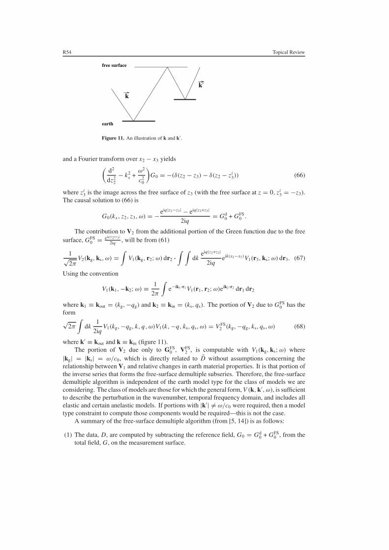
V1(k′g, r2, ω)G0(r2, r3, ω)V1(r3, ks, ω) dr2 dr3. (61)
Expressing G0 as a Fourier transform over x2 − x3, we find
G0(x2 − x3, z2, z3; ω) = 1√2π
∫dk G0(k, z2, z3; w)eik(x2−x3) (62)
and
G0(k, z2, z3; ω) = 1√2π
∫e−ikx dx G0(x, z2, z3; ω). (63)
For G0 = Gd0, (63) reduces to
Gd0(k, z2, z3; ω) = −eiq|z2−z3|
2iq(64)
where
q =√(
ω
c0
)2
− k2.
For the marine case where there is a free surface, the Green function G0 satisfies(∇2 +
ω2
c20
)G0 = −(δ(r2 − r3) − δ(r2 − ri
3)) (65)
R54 Topical Review
earth
free surface
k
k′
Figure 11. An illustration of k and k′.
and a Fourier transform over x2 − x3 yields(d2
dz22
− k2x +
ω2
c20
)G0 = −(δ(z2 − z3) − δ(z2 − zi
3)) (66)
where zi3 is the image across the free surface of z3 (with the free surface at z = 0, zi
3 = −z3).The causal solution to (66) is
G0(kx, z2, z3, ω) = −eiq|z2−z3| − eiq|z2+z3|
2iq= Gd
0 + GFS0 .
The contribution to V2 from the additional portion of the Green function due to the freesurface, GFS
0 = eiq|z2+z3 |2iq , will be from (61)
1√2π
V2(kg, ks, ω) =∫
V1(kg, r2; ω) dr2 ·∫ ∫
dkeiq|z2+z3|
2iqeik(x2−x3)V1(r3, ks; ω) dr3. (67)
Using the convention
V1(k1,−k2; ω) ≡ 1
2π
∫e−ik1·r1 V1(r1, r2; ω)eik2·r2 dr1 dr2
where k1 ≡ kout = (kg,−qg) and k2 ≡ kin = (ks, qs). The portion of V2 due to GFS0 has the
form√
2π
∫dk
1
2iqV1(kg,−qg, k, q, ω)V1(k,−q, ks, qs, ω) = V FS
2 (kg,−qg, ks, qs, ω) (68)
where k′ ≡ kout and k ≡ kin (figure 11).The portion of V2 due only to GFS
0 , VFS2 , is computable with V1(kg, ks; ω) where
|kg| = |ks| = ω/c0, which is directly related to D without assumptions concerning therelationship between V1 and relative changes in earth material properties. It is that portion ofthe inverse series that forms the free-surface demultiple subseries. Therefore, the free-surfacedemultiple algorithm is independent of the earth model type for the class of models we areconsidering. The class of models are those for which the general form, V (k, k′, ω), is sufficientto describe the perturbation in the wavenumber, temporal frequency domain, and includes allelastic and certain anelastic models. If portions with |k′| = ω/c0 were required, then a modeltype constraint to compute those components would be required—this is not the case.
A summary of the free-surface demultiple algorithm (from [5, 14]) is as follows:
(1) The data, D, are computed by subtracting the reference field, G0 = Gd0 + GFS
0 , from thetotal field, G, on the measurement surface.
Topical Review R55
(2) Compute the deghosted data, D where D = D/[(e2iqgεg − 1)(e2iqsεs − 1)], from D and thesource and receiver deghosting factors in the k–ω domain, Gd
0/G0 = 1/(e2iqε − 1). qs,qg and εs, εg are the vertical wavenumbers and the depths below the free surface of thesource and receiver, respectively.
(3) The series for deghosted and free-surface demultipled data, D′, is given in terms of thedeghosted data D′
1 as follows:
D′n(kg, ks, ω) = 1
iπρ0 B(ω)
∫ ∞
−∞dk qeiq(εg+εs) D′
1(kg, k, ω)D′n−1(k, ks, ω),
n = 2, 3, 4, . . . , (69)
and
D′(kg, ks, ω) =∞∑
n=1
D′n(kg, ks, ω) (70)
where D′(kg, ks, ω) ≡ D′(kg, εg, ks, εs, ω), B(ω) and ρ0 are the source signature andreference density, respectively. The data D′ consist of deghosted primaries and internalmultiples only and D′
1 = D. Hence, D′ represents the deghosted data without free-surface multiples. The mathematical details of (69) and (70) follow from (11′)–(13′) andare provided in [14] and [5]. Equations (69) and (70) are the prestack multi-dimensionalgeneralizations of the one dimensional, normal incidence free-surface-elimination mappresented in the appendix of [26].
A rigorous integral equation formulation relating data with free surface events to datawithout those events is derived by Fokkema and van den Berg [27]. A series expansionsolution of the latter integral equation agrees exactly with the inverse scattering free-surfacemultiple removal subseries represented by (69) and (70). A feedback loop method for free-surface multiple removal was also described by Berkhout [28]. The differences between theinverse subseries for free-surface multiple removal and the feedback method are discussed inthe section on data examples.
6. Internal multiple attenuation
6.1. The subseries that attenuates internal multiples
In the previous section, we described how to achieve the goal of separating the removal ofsurface multiples from the other three tasks of inversion. We now address the more difficultissue of separating the task of attenuating internal multiples from the last two goals of migrationand inversion of primaries.
When we separated surface multiples from the other three goals we were able to isolatea portion of the Green function, G0, namely GFS
0 , whose purpose in the forward and inverseseries was to produce and remove, respectively, events due to the presence of the free surface.Unfortunately, for internal multiples, we do not have that relatively straightforward road tofollow.
If we attempt to repeat the reasoning that proved useful with surface multiples, we seek anexample that has neither free-surface nor internal multiples. We can imagine a problem wherewe have two half-spaces; that is, we wish to invert a model that has only a single horizontalreflector. In that case, the scattered field, the primary, requires for its description a completeforward scattering series in terms of Gd
0 and the exact perturbation, V. The inverse series for Vin terms of the data, the primary, requires the full series and Gd
0. The lesson, from this singlereflector example, is that the complete Gd
0 is required in the inverse series when the only tasks

R56 Topical Review
are locating reflectors and estimating parameters. Hence, we cannot separate Gd0 into an extra
part that exists only in the presence of internal multiples, but which is not present when internalmultiples are absent. Thus, a fundamentally different approach is required for the attenuationof internal multiples.
We next present the logical path that leads to this new approach. The forward seriesgenerates primaries and internal multiples through the action of Gd
0 on V. The inverse seriesconstructs V from the action of Gd
0 on the recorded data. The action of Gd0 on data must
remove internal multiples on the way to constructing V. In an earlier section, we presented ananalysis and interpretation of the forward series and, specifically, how Gd
0 generates primariesand internal multiples of a given order. However, before we focus on the internal multipleissue, it is important to note an essential difference between the scattering theory pictures offree-surface and internal multiple generation.
Given data, D′, without free-surface events, the forward series generates data, D, withfree-surface events by the action of GFS
0 on D′. Each term in that series generates one orderof free-surface multiple—that is, all events that have reflected from the free surface a givennumber of times. The modelling that GFS
0 provides is an exact description of a wave propagatingin the water and reflecting from the free surface. Hence, GFS
0 generates in the forward seriesand removes in the inverse series one order of free-surface multiple with each term.
The situation for primaries and internal multiples is quite different. For those events, weadopt a point-scatterer model, and every term in that forward series contributes to (but does notby itself fully describe) either primary or internal multiples. Each primary or internal multiplerequires an infinite series for its construction. We adopt the simpler surface reflection modelwhen describing wave phenomena associated with reflectors at or above the measurementsurface; we adopt the point-scatterer model for waves associated with subreceiver/sourcestructure. The former is our model of choice when we have accurate or nearly accurateinformation about velocities and structure and the latter is our model when that information isunavailable or unreliable.
The location and properties of the free surface are captured in GFS0 and it is that specific
and well-defined free surface reflection experience (or its absence) which allows free-surfacemultiples to be separated from primaries and internal multiples with one term creating (in theforward series) and one term removing (in the inverse series) all events that have experiencedthe free surface a given number of times. The number of GFS
0 factors in a term in thesubseries (12′), (13′) corresponds to the order of free-surface multiples that it removes. Theinternal multiples have (by definition) all of their downward reflections below the free surfaceand since we assume absolutely no subsurface information those reflectors are assumed to becompletely unknown in both location and character.
This makes the problem of distinguishing the generation (and removal) of internalmultiples from primaries more difficult in terms of direct propagation through water, Gd
0, andthe difference between earth and water properties, V. As mentioned earlier, a series is requiredto generate any primary or any internal multiple in terms of Gd
0 and V and new concepts arerequired to distinguish the forward subseries for constructing primaries from the subseries forinternal multiples and then to conjecture on how to separate the tasks that act on these eventsin the inverse series.
It is no surprise that the first term in the forward series that constructs and first term inthe inverse series that eliminates internal multiples of a given order are approximate. Theefficiency of the first term in the removal subseries of internal multiples is remarkably higherthan the first term in the forward creation; e.g., it takes an infinite series to get the importanttime prediction (phase) of any internal multiple in the forward series (in terms of Gd
0 and V)whereas, as we will demonstrate, the first term in the removal series (of an internal multiple

Topical Review R57
(a) (b)
Figure 12. The leading term contribution to the generation of first order internal multiples isrepresented in (a) and suggests the leading term contribution, in the inverse series, to the removalof first order internal multiples represented in (b). Gd
0, V and V1 are the whole-space Green function,the perturbation operator and the ‘migrated data-like’ first order approximation to V, respectively.
of a given order) predicts the time precisely and approximates well the amplitude (in termsof Gd
0 and D′) of all multiples of that order—from all reflectors at all depths at once. Theefficiency of the first term of the inverse subseries for internal multiple elimination accountsfor its practical value and impact.
The fact that generating primaries and internal multiples of a given order requires aninfinite series suggests that an infinite series of terms, each involving operations with Gd
0 onD′, is required to remove internal multiples of a given order. The particular inverse scatteringsubseries for attenuating all internal multiples, described here, chooses only the leading andmost significant contribution from the removal series of each order of multiple, forming aseries that attenuates well, rather than eliminates, all internal multiples.
In our earlier discussion of the forward series for primaries and internal multiples weargued that primaries are constructed starting with the first term in the series and that firstorder internal multiples have their leading contribution in the third term. Similarly, secondorder internal multiples are generated by contributions starting with the fifth term in the forwardseries. In general, nth order internal multiples have contributions from all terms starting atterm 2n + 1. In addition, the portion of the third term that starts to build the first order internalmultiple was distinguished from the part that has a third order contribution to constructingprimaries. The leading term contribution to constructing a class of multiples in the forwardseries suggests the leading term contribution for their removal in the inverse series (figure 12).
The first two terms in the forward series do not contribute to generating first order internalmultiples. Similarly, it is argued that the first two terms in the inverse series do not contributeto their removal. The mathematical realization of figure 12(a) is the leading contribution tothe generation of first order internal multiples; it suggests the corresponding mathematicalexpression for the leading order attenuation of those multiples. To realize, or algorithmicallycapture the physics associated with figure 12(b), select the portion of the third term of theinverse series with z1 > z2 and z3 > z2.
With this purpose in mind we examine V3, the third term in the inverse series. In contrastwith the subseries generated by GFS
0 , for free-surface multiple attenuation (13′), the threeterms in V3 do not sum to a single term when the inverse series is generated with the directpropagating Green function, Gd
0. From the fact that GFS0 can be viewed as the Green function
due to an image source above the free surface and is therefore outside the volume, it followsthat for all z, z′ inside the volume (i.e., below the free surface) GFS
0 satisfies the homogeneousdifferential equation(∇2
ρ0+
ω2
K0
)GFS
0 = 0.
R58 Topical Review
The fact that GFS0 satisfies a homogeneous differential equation leads in turn to the mathematical
simplification
(Gd0V1GFS
0 V1GFS0 V1Gd
0)m = −(Gd0V1GFS
0 V2Gd0)m
= −(Gd0V2GFS
0 V1Gd0)m. (71)
In computing (71), GFS0 does not require an off-shell k = k′ contribution since its effective
source (the image source) is, by definition, outside the volume supporting V1 and V2 and,hence, outside the integrals that compute terms in that particular subseries. This gives anotherway to understand why the free-surface demultiple algorithm is automatically model typeindependent. Model type was needed by Razavy [12] to provide T1(k, p) for k = p. SinceGFS
0 never requires k = p in its integrations with V1, it does not depend upon the inverse seriesmodel type argument to generate this subseries. Hence the free-surface multiple removalsubseries is independent of the earth model type. In contrast, Gd
0 satisfies the inhomogeneousdifferential equation(∇2
ρ0+
ω2
K0
)Gd
0 = −δ(z − z′)δ(x − x ′).
From (13′′) and using Gd0, we have:
(Gd0V3Gd
0) = −(Gd0V1Gd
0V2Gd0) − (Gd
0V2Gd0V1Gd
0) − (Gd0V1Gd
0V1Gd0V1Gd
0)
= (Gd0V31Gd
0) + (Gd0V32Gd
0) + (Gd0V33Gd
0), (72)
where
V31 ≡ −V1Gd0V2, (73)
V32 ≡ −V2Gd0V1, (74)
and
V33 ≡ −V1Gd0V1Gd
0V1. (75)
In contrast to the case for GFS0 , these three terms V31, V32 and V33 make distinct contributions.
The first two terms, (Gd0V31Gd
0) and (Gd0V32Gd
0), in the right member can be shown [29]to always contain a refraction-like (i.e., not reflection-like) scattering component and arethus not involved with the task of removing internal multiples. We define a reflection-likescattering (or inverse scattering) as one that changes its propagation direction with respectto the measurement surface after the interaction with V (or V1). Refraction-like scatteringcontributions in V3 contribute to the other inversion tasks (migration and inversion) that act onprimaries. The third term on the right-hand side,
(Gd0V33Gd
0) = −(Gd0V1Gd
0V1Gd0V1Gd
0),
can be broken up into four parts corresponding to the four diagrams in figure 13.Choose the portion of (Gd
0V33Gd0)m corresponding to figure 13(d); a diagram that
represents a contribution to multiple reflection attenuation. (Gd0V31Gd
0)m and (Gd0V32Gd
0)m
do not support a diagram of the figure 13(d) variety and therefore were not selected for thattask. The mathematical and algorithmic realizations of figure 13(d) take place on requiringa lower–higher–lower relationship between the successive vertical locations of the data inthe integral. Using this criterion, the appropriate portion of each of the odd terms in theseries is selected. The generalization of the diagram found in figure 13(d) is used to selectthe appropriate portion of the leading order contribution to removing higher order internalmultiples.
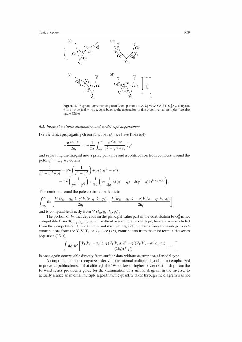
Topical Review R59
(a)
(c) (d)
(b)
Figure 13. Diagrams corresponding to different portions of sGd0V1Gd
0V1Gd0V1Gd
0g. Only (d),with z1 > z2 and z2 < z3, contributes to the attenuation of first order internal multiples (see alsofigure 12(b)).
6.2. Internal multiple attenuation and model type dependence
For the direct propagating Green function, Gd0, we have from (64)
−eiq|z2−z3|
2iq= − 1
2π
∫ ∞
−∞eiq ′(z2−z3)
q2 − q ′2 + iεdq ′
and separating the integral into a principal value and a contribution from contours around thepoles q ′ = ±q we obtain
1
q2 − q ′2 + iε= PV
(1
q2 − q ′2
)+ iπδ(q ′2 − q2)
= PV
(1
q2 − q ′2
)+
1
2π
(iπ
1
2|q|(δ(q′ − q) + δ(q ′ + q))eiq ′(z2−z3)
).
This contour around the pole contribution leads to∫ ∞
−∞dk
[V1(kg,−qg, k, q)V1(k, q, ks, qs)
2iq+
V1(kg,−qg, k,−q)V1(k,−q, ks, qs)
2iq
]
and is computable directly from V1(kg, qg, ks, qs).The portion of V2 that depends on the principal value part of the contribution to Gd
0 is notcomputable from �s(xg, εg, xs, εs, ω) without assuming a model type; hence it was excludedfrom the computation. Since the internal multiple algorithm derives from the analogous iπδ
contributions from the V1V1V1 or V33 (see (75)) contribution from the third term in the series(equation (13′′)),∫
dk dk ′[
V1(kg,−qg, k, q)V1(k, q, k ′,−q ′)V1(k ′,−q ′, ks, qs)
(2iq)(2iq ′)+ · · ·
]
is once again computable directly from surface data without assumption of model type.An important point to recognize in deriving the internal multiple algorithm, not emphasized
in previous publications, is that although the ‘W’ or lower–higher–lower relationship from theforward series provides a guide for the examination of a similar diagram in the inverse, toactually realize an internal multiple algorithm, the quantity taken through the diagram was not
R60 Topical Review
V1 but rather b1: the effective data generated by a single frequency plane-wave incident fieldgiven by
b1(kg, εg, ks, εs, qg + qs) = (−2iqs)D′(kg, εg, ks, εs, ω) = V1(kg, qg, ks, qs, ω)
−2iqg.
This was originally deduced through empirical evaluation and testing of different candidatequantities (e.g. a first and natural guess of taking V1 through ‘W’ does not lead to an attenuationalgorithm) that, in turn, allow different subdivisions of the V33 term in terms of a ‘W’diagram [5, 29].
The fact that b1 results in localized incident and scattered (reflected) wavefronts in everydimension (without the wake behind the wavefront in the 1D and 2D impulse responserepresented by D′) is the only and best understanding or hint we have for this fact to date. Thatis, it seemed that the internal multiple attenuation algorithm favoured a quantity to be takenthrough the ‘W’ diagram that in every dimension would correspond to a scattered field with allspike-like or localized events. Neither V1 nor D′ satisfies that criterion in every dimension, but−2iqs D′ does. Hence, the forward construction and inverse removal ‘W’ diagram symmetry forthe internal multiple went only so far and the fact that b1 is the quantity that when transformedto (kg, qg, z) and broken into lower–higher–lower contributions results in the internal multiplealgorithm remains partly intuitive and empirical in its foundation and invites further physicalinterpretation and mathematical analysis. A deeper comprehension of the workings of theinverse series will also benefit the current research on imaging and inverting primaries.
The internal multiple attenuation algorithm operates in a 1D, 2D or 3D earth and isindependent of the model type because it derives from a algorithm depending on the portionof V1 and V3 that only requires |kg| = |ks| = ω/c0.
The inverse scattering series is not computable for a general operator of the form V(p, k, ω)
where the vectors p and k have the same dimension as the subsurface, e.g., they are threedimensional vectors for a three dimensional earth, but are otherwise independent of each otherand ω. However, the subseries of the inverse series for V(p, k, ω) that results from only theiπδ contributions, where |p| = |k| = ω/c0, is directly computable without assuming a modeltype. When seeking model type-independent algorithms (as is the case for the free-surfacedemultiple algorithm), you either demonstrate that the principal value contribution is zero,or in the case of the internal multiple attenuation algorithm you choose from the beginningonly the portion of the inverse series to task subdivide that is independent of model type. Amodel type-independent task-specific subseries provides a selection criterion for seeking andisolating certain terms and ignoring others.
We anticipate that the refraction-like inverse-scattering contributions that play a role inimaging primaries at depth and progressing from internal multiple attenuation to eliminationwill be model type independent when either the measured wavefield contains both reflection andtransmission data (e.g., surface reflection and vertical seismic profiles) or when transmissiondata can be constructed from reflection data. The fourth task, that of earth mechanical propertiesidentification, will certainly require specification of what set of parameters you seek to identifyand will therefore be model-type specific. That three of the four tasks associated with inversionwould be model-type independent speaks to the conceptual and practical value of that approachand strategy.
6.3. Internal multiple attenuation algorithm
The first term in the internal multiple attenuation subseries is the data, D′, consisting ofprimaries and internal multiples. The second term in this series comes from a portion of the

Topical Review R61
third term in the inverse series ((72) and (75)). This portion of the third term,
b3(kg, ks, qg + qs) = 1
(2π)2
∫ ∞
−∞
∫ ∞
−∞dk1 e−iq1(εg−εs) dk2 eiq2(εg−εs)
×∫ ∞
−∞dz1 ei(qg+q1)z1b1(kg, k1, z1)
∫ z1
−∞dz2 ei(−q1−q2)z2 b1(k1, k2, z2)
×∫ ∞
z2
dz3 ei(q2+qs)z3 b1(k2, ks, z3), (76)
is chosen to satisfy z1 > z2 and z2 < z3. b1 is defined in terms of the original prestack datawith free-surface multiples eliminated, D′, and is defined by
D′(kg, ks, ω) = (−2iqs)−1 B(ω)b1(kg, ks, qg + qs) (77)
where B(ω) is the source signature and, once again, b1 represents the data that would resultfrom a single frequency incident plane wave. The data with internal multiples attenuated, DIM,are
DIM(kg, ks, ω) = (−2iqs)−1 B(ω)
∞∑n=0
b2n+1(kg, ks, qg + qs) (78)
where DIM contains the primaries with their wavelet. A recursive relationship thatgeneralizes (78) and provides b2n+1 in terms of b2n−1 for n = 1, 2, 3, . . . is given in [29]as
b2n+1(kg, ks, qg + qs) = 1
(2π)2n
∫ ∞
−∞dk1 e−iq1(εg−εs)
×∫ ∞
−∞dz1 ei(qg+q1)z1b1(kg, k1, z1)A2n+1(k1, ks, z1),
n = 1, 2, 3, . . . , (79)
where
A3(k1, ks, z1) =∫ ∞
−∞dk2 eiq2(εg−εs)
∫ z1
−∞dz2 ei(−q1−q2)z2 b1(k1, k2, z2)
×∫ ∞
z2
dz3 ei(q2+qs)z3b1(k2, ks, z3)
and
A2n+1(k1, ks, z1) =∫ ∞
−∞dk2 eiq2(εg−εs)
∫ z1
−∞dz2 ei(−q1−q2)z2 b1(k1, k2, z2)
×∫ ∞
−∞dk3 e−iq3(εg−εs)
∫ ∞
z2
dz3 ei(q2+q3)z3
× b1(k2, k3, z3)A2n−1(k3, ks, z3), n = 2, 3, 4, . . . .
As we mentioned, the full series for V can have restrictive convergence properties (see,e.g., [14]). In contrast, numerical tests indicate that the internal multiple attenuation subseriesin (79) always converges and is insensitive to missing low frequency information [29–31].
Free-surface multiple attenuation methods operate one temporal frequency at a time(see (69) and (70)); in contrast, the attenuation of an internal multiple from a single frequencyof data requires data at all frequencies (see (78) and (79)). This requirement derives fromthe integral over temporal frequency in the transform of qg + qs to z. With band-limited datathis transform is only approximate; nevertheless, the truncated integral remains effective atattenuating multiples. As in the case of the free-surface multiple removal algorithm, each term

R62 Topical Review
in the series in (78) attenuates a given order of internal multiple and prepares the higher orderinternal multiples for the higher order demultiple terms in the series. Since eikz zb1(kg, ks, ω)
is a downward continuation of shots and receivers to depth z in the reference medium andsubsequent integration over kz is a simple constant Jacobian away from integration over ω
(t = 0 imaging condition), it follows that b1(kg, ks, z) corresponds to uncollapsed migration[3, 32]. Indeed, the algorithm can be interpreted as a sequence of these uncollapsed migrationsrestricted to lower–higher–lower pseudo-depths.
Pseudo-depth and migration are terms often used in exploration geophysics. Pseudo-depth refers to the location of an image derived using the background reference velocity.Since the reference velocity is constant (water), pseudo-depth is essentially vertical traveltime. Migration refers to the imaging process where subsurface reflectors are ‘migrated’from the incorrect to the correct location. Uncollapsed migration is a generalization of theoriginal migration concept; sources and receivers are downward continued to a common depthlevel z, time is evaluated at zero and information at xg = xs is retained. The latter retention ofxg = xs distinguishes uncollapsed migration from migration; it provides local angle-dependentreflection coefficients rather than the angle-averaged reflection coefficient of the traditionalxg = xs imaging condition (see [32]).
The process of obtaining a primaries-only data set starts with D: a data set with free-surfaceand internal multiples and primaries. D is then input into the free-surface demultiple algorithmto produce D′, which is then used as input to the internal multiple attenuation algorithm tooutput data that contain primaries.
7. Analytic, numerical and field data examples of free-surface and internal multipleattenuation
7.1. Purposeful perturbation
As we have described, the combination of the apparent lack of robust convergence of the entireinverse series, without a level of a priori information that is generally not achievable, and therecognition that it nevertheless represented the only complete inversion formalism for multi-dimensional acoustic and elastic waves motivated the search for task-specific subseries thatwould have more favourable properties. At the same time, another issue that these task-specificand well-converging subseries faced was how many terms would be required in practice toachieve a certain level of effectiveness towards the specific task associated with that subseries.The concept of purposeful perturbation was developed to address the latter issue.
The idea is to identify the specific purpose or role that each term within a task-specificsubseries performs independent of the subsurface or target over which the recorded data werecollected.
The terms of the series perform uncoupled and coupled tasks; the task-specific subseriesperform isolated, uncoupled tasks. We define the purposeful perturbation concept as knowledgeof precisely what each term within a given task-specific subseries is designed to accomplish.For example, a term in the inverse scattering subseries for eliminating free-surface multiplesremoves precisely one order of free-surface multiple completely independent of the depth ofthe water or any other property or characteristic of the earth.
7.2. 1D free-surface demultiple algorithm (example of purposeful perturbation)
If the subseries that we isolate accomplishes one of the four broad tasks (described insection 2.5), then purposeful perturbation further determines and defines the specific role or

Topical Review R63
Figure 14. An illustration of the free-surface multiple removal series: (a) data without a freesurface, (b) the total upgoing field in the presence of a free surface RFS and (c) the series for RFSin terms of R.
subtask that individual terms in that subseries perform in completing the overall task associatedwith that subseries. For example, if you estimate the range of depths of potential hydrocarbonreservoirs in a given setting and the depth to the water bottom is known, then you have a goodway to determine the highest order of water bottom multiple that you need to be concernedwith and precisely the number of terms in the free-surface demultiple subseries ((69) and (70))that can accomplish that objective.
For the simplest illustration of this purposeful perturbation concept, consider thegeneration of free-surface multiples for a 1D earth, whose primary reflections and internalmultiples have a response R(ω); and, where the free surface is characterized by a reflectioncoefficient of −1 for a pressure wavefield (see figure 14).
For source and receiver deghosted data and a source wavelet with unit amplitude, theupgoing field in the presence of a free surface RFS is able to be written in terms of R(ω) byimagining (see figure 14 (c)) the wave first leaving the source moving down into the earth; thatincident unit pressure wave generates a reflected response from the earth, R(ω), consistingof primaries and internal multiples. This in turn propagates as a train up through the watercolumn until it hits the free surface, where it experiences a −1 reflection coefficient and headsdown through the water columns as −R(ω) and is incident upon the earth as a long ‘wavelet’.The impulse response of the earth R(ω) times this effective downgoing ‘wavelet’, −R(ω),produces a new wave moving up from the earth through the water column towards the freesurface. This process continues and results in the total upgoing wave in the presence of the freesurface, RFS(ω), in terms of the primary and internal multiple wavefield, R(ω), as follows:
RFS = R − R2 + R3 − · · ·= R
1 + R. (80)
Each term in (80) generates all free-surface multiples of a given order independent of anydetail of the subsurface. The order of a free-surface multiple corresponds to the number oftimes that event has experienced a reflection at the free surface. Since each successive termin (80) comes from one additional reflection at the free surface, it generates one additionalorder of free-surface multiple. If you were interested in creating free-surface multiples up to agiven order, then understanding the purpose of each term in (80) allows you to know preciselyhow many terms that objective would require. Solving (80) for the data without free-surfacemultiples, R, we have
R = RFS
1 − RFS
= RFS + R2FS + R3
FS + · · · . (81)

R64 Topical Review
The first term in (81), RFS, is the upgoing portion of the reflection data that contains allprimaries, internal multiples and free-surface multiples. When the second term, R2
FS, is addedto RFS two things happen: (1) all free-surface multiples that have reflected once (and onlyonce) from the free surface are removed and (2) all higher order free-surface multiples arealtered in preparation for higher terms, e.g., R3
FS, to remove them order by order, as well. Thiswell-defined action of the terms in the free-surface demultiple series is totally independent ofany water bottom or subsurface detail (of course, within an assumed 1D, 2D or 3D dimensionof the earth variation).
This is an example of purposeful perturbation; and it has enormous practical significance.For example, if you estimate that for a given depth of water and target, only a certain orderof multiples could be troublesome, then you know precisely how many terms in the seriesyou need to use in your processing algorithm for that data. Equation (81) is the 1D normalincidence special case of the general multi-dimensional inverse scattering subseries for free-surface multiple removal (69) and (70) (see also [5, 14]).
Equation (81) is the 1D antecedent of (11′) to (13′), (69) and (70) for free-surface multipleremoval. Several observations about equations (80) and (81) are worth noting. First, therole of GFS
0 , the extra portion of G0 due to the free surface is played by the (−1) reflectioncoefficient in deriving (80) and its inverse (81). Second, the forward construction series wasa guide (and in this simple instance, more than a guide) to the inverse process. Only the free-surface reflection coefficient (−1) terms enter (i.e., GFS
0 ) confirming the forward and removalseries (80) and (81), respectively. Focusing on only this single task, we see that no coupledterms in GFS
0 , Gd0 appear in the analogous and transparently simple (80) and (81), which is
consistent with, and supports, the strategy that we described for the generalized algorithm thatderives from the multi-dimensional inverse series.
Regarding some practical issues, if instead of a unit incident pulse a wavelet A(ω) wasthe source signature, then (80) would become
RFS = A(ω)R
1 + R(82)
and (81) becomes
R =RFS
A(ω)
1 − RFSA(ω)
= RFS
A(ω)+
(RFS
A(ω)
)2
+ · · · (83)
and, hence, the wavelet is a critical requirement for the free-surface multiple removal and allsubseries application (see, e.g., [33–35]).
A similar process of purposeful perturbation occurs (and has been identified) for theinternal multiple removal series. Understanding the specific purpose of each term within anoverall task reveals what has (and has not) been achieved for a given finite number of termsproviding a critically important practical guide for field data application as well as mitigatingissues of overall convergence and rate of convergence.
7.3. 1D analytic example of the internal multiple attenuation algorithm
The 2D internal multiple algorithm is described in (76)–(79). The first term in this series is
b(kg, ks, qg + qs) = −2iqs D′(kg, ks, ω)
where D′ represents the data resulting from an impulsive source and after free-surface multipleremoval. The second term in this series is b3, given by

Topical Review R65
Figure 15. A one dimensional model with two interfaces.
b3(kg, ks, qg + qs) = 1
(2π)2
∫ ∞
−∞
∫ ∞
−∞dk1 eiq1(εs−εg) dk2 eiq2(εg−εs)
×∫ ∞
−∞dz1 ei(qg+q1)z1b1(kg,−k1, z1)
∫ z1
−∞dz2 ei(−q1−q2)z2 b1(k1,−k2, z2)
×∫ ∞
z2
dz3 ei(q2+qs)z3 b1(k2,−ks, z3).
The first two terms in the internal multiple attenuation series attenuate all first order internalmultiples. For a 1D earth and a normal incidence plane wave, (76) reduces to
b3(k) =∫ ∞
−∞dz1 eikz1 b(z1)
∫ z1
∞dz2 e−ikz2 b(z2)
∫ ∞
z2
dz3 eikz3 b(z3). (84)
To explicitly demonstrate how the internal multiple attenuation algorithm works and toexamine its properties, we will consider the simplest model that can produce an internalmultiple. For the model shown in figure 15 the reflection data due to an impulsive incidentwave δ(t − z
c ) are
D′(t) = R1δ(t − t1) + T01 R2T10δ(t − t2) + · · ·where t1, t2, R1, R2 are the two way times and reflection coefficients from the two reflectorsand T01 and T10 are the coefficients of transmission between model layers 0 and 1 and 1 and 0,respectively;
D′(ω) = R1eiωt1 + T01 R2T10eiωt2 + · · · (85)
where D′(ω) is the temporal Fourier transform of D′(t).Note that the (−2iqs) factor that multiplies D′ in the internal multiple theory is not required
in this example since we assume that the incident wave is an impulsive plane wave. The roleof (−2iqs) is to transform an incident (or reference field) G0 into a plane wave in the Fourierdomain. The input into the internal multiple algorithm is b: data with primaries and internalmultiples. This is also the first term in the multiple attenuation series, thus b1 = b and
bIM(k) = b1(k) + b3(k) + b5(k) + · · · .The vertical wavenumber is
kz =√
(ω/c0)2 − k2xg
+√
(ω/c0)2 − k2xs
and for a 1D medium and a normal incident wave it is kz = 2 ωc0
and
b(kz) = D(ω). (86)
The reflection data from (85) and (86) are expressed in terms of kz:
b(kz) = R1 exp
(i
(2ω
c0
)(c0t1
2
))+ T01 R2T10 exp
(i
(2ω
c0
)(c0t2
2
))+ · · · (87)
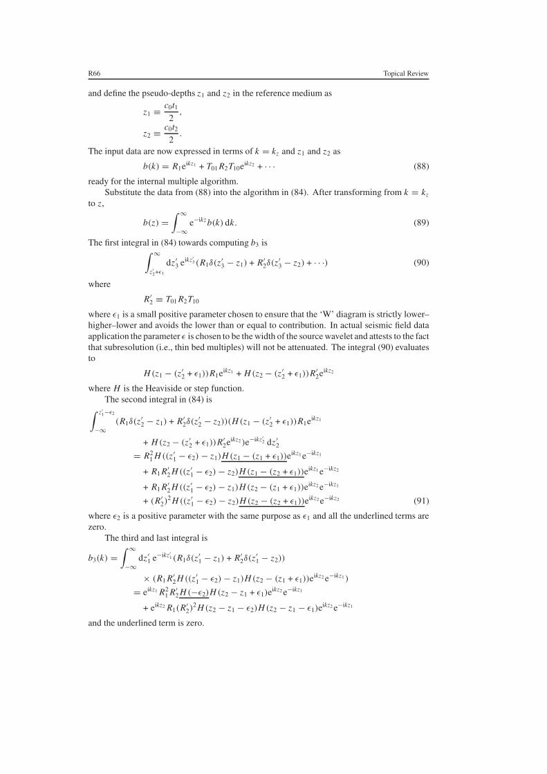
R66 Topical Review
and define the pseudo-depths z1 and z2 in the reference medium as
z1 ≡ c0t12
,
z2 ≡ c0t22
.
The input data are now expressed in terms of k = kz and z1 and z2 as
b(k) = R1eikz1 + T01 R2T10eikz2 + · · · (88)
ready for the internal multiple algorithm.Substitute the data from (88) into the algorithm in (84). After transforming from k = kz
to z,
b(z) =∫ ∞
−∞e−ikzb(k) dk. (89)
The first integral in (84) towards computing b3 is∫ ∞
z′2+ε1
dz′3 eikz′
3(R1δ(z′3 − z1) + R′
2δ(z′3 − z2) + · · ·) (90)
where
R′2 ≡ T01 R2T10
where ε1 is a small positive parameter chosen to ensure that the ‘W’ diagram is strictly lower–higher–lower and avoids the lower than or equal to contribution. In actual seismic field dataapplication the parameter ε is chosen to be the width of the source wavelet and attests to the factthat subresolution (i.e., thin bed multiples) will not be attenuated. The integral (90) evaluatesto
H (z1 − (z′2 + ε1))R1eikz1 + H (z2 − (z ′
2 + ε1))R′2eikz2
where H is the Heaviside or step function.The second integral in (84) is∫ z′
1−ε2
−∞(R1δ(z
′2 − z1) + R′
2δ(z′2 − z2))(H (z1 − (z ′
2 + ε1))R1eikz1
+ H (z2 − (z ′2 + ε1))R′
2eikz2 )e−ikz′2 dz′
2
= R21 H ((z ′
1 − ε2) − z1)H (z1 − (z1 + ε1))eikz1 e−ikz1
+ R1 R′2 H ((z ′
1 − ε2) − z2)H (z1 − (z2 + ε1))eikz1 e−ikz2
+ R1 R′2 H ((z ′
1 − ε2) − z1)H (z2 − (z1 + ε1))eikz2 e−ikz1
+ (R′2)
2 H ((z ′1 − ε2) − z2)H (z2 − (z2 + ε1))eikz2 e−ikz2 (91)
where ε2 is a positive parameter with the same purpose as ε1 and all the underlined terms arezero.
The third and last integral is
b3(k) =∫ ∞
−∞dz′
1 e−ikz′1(R1δ(z
′1 − z1) + R′
2δ(z′1 − z2))
× (R1 R′2 H ((z ′
1 − ε2) − z1)H (z2 − (z1 + ε1))eikz2 e−ikz1 )
= eikz1 R21 R′
2 H (−ε2)H (z2 − z1 + ε1)eikz2 e−ikz1
+ eikz2 R1(R′2)
2 H (z2 − z1 − ε2)H (z2 − z1 − ε1)eikz2 e−ikz1
and the underlined term is zero.
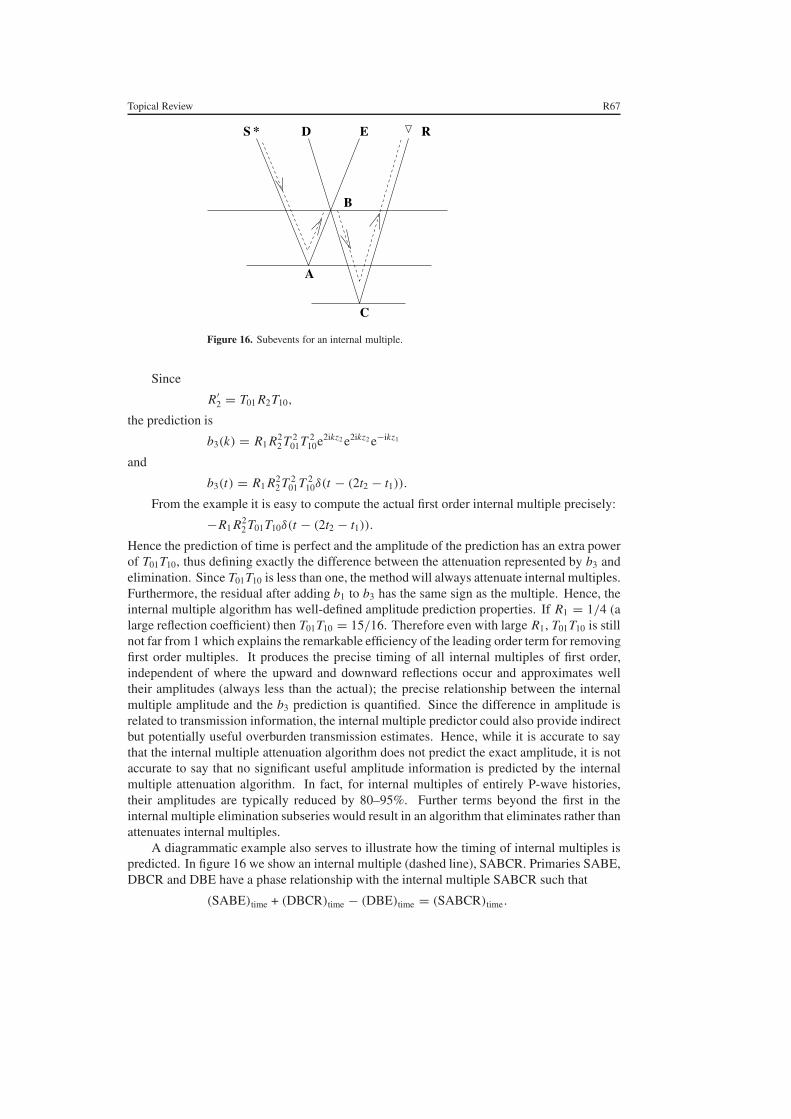
Topical Review R67
Figure 16. Subevents for an internal multiple.
Since
R′2 = T01 R2T10,
the prediction is
b3(k) = R1 R22 T 2
01T 210e2ikz2 e2ikz2 e−ikz1
and
b3(t) = R1 R22 T 2
01T 210δ(t − (2t2 − t1)).
From the example it is easy to compute the actual first order internal multiple precisely:
−R1 R22 T01T10δ(t − (2t2 − t1)).
Hence the prediction of time is perfect and the amplitude of the prediction has an extra powerof T01T10, thus defining exactly the difference between the attenuation represented by b3 andelimination. Since T01T10 is less than one, the method will always attenuate internal multiples.Furthermore, the residual after adding b1 to b3 has the same sign as the multiple. Hence, theinternal multiple algorithm has well-defined amplitude prediction properties. If R1 = 1/4 (alarge reflection coefficient) then T01T10 = 15/16. Therefore even with large R1, T01T10 is stillnot far from 1 which explains the remarkable efficiency of the leading order term for removingfirst order multiples. It produces the precise timing of all internal multiples of first order,independent of where the upward and downward reflections occur and approximates welltheir amplitudes (always less than the actual); the precise relationship between the internalmultiple amplitude and the b3 prediction is quantified. Since the difference in amplitude isrelated to transmission information, the internal multiple predictor could also provide indirectbut potentially useful overburden transmission estimates. Hence, while it is accurate to saythat the internal multiple attenuation algorithm does not predict the exact amplitude, it is notaccurate to say that no significant useful amplitude information is predicted by the internalmultiple attenuation algorithm. In fact, for internal multiples of entirely P-wave histories,their amplitudes are typically reduced by 80–95%. Further terms beyond the first in theinternal multiple elimination subseries would result in an algorithm that eliminates rather thanattenuates internal multiples.
A diagrammatic example also serves to illustrate how the timing of internal multiples ispredicted. In figure 16 we show an internal multiple (dashed line), SABCR. Primaries SABE,DBCR and DBE have a phase relationship with the internal multiple SABCR such that
(SABE)time + (DBCR)time − (DBE)time = (SABCR)time.

R68 Topical Review
Multiples
Input data stackInternal multiple
estimate stack Output data stack
Primaries
0
1
2
3
Seco
nds
Figure 17. A 2D synthetic model (top). The left panel (bottom) shows a common offset displayfrom the synthetic data set created using the model. The middle panel (bottom) shows the predictedinternal multiples and the right-hand panel (bottom) is the result after subtracting the predictedmultiples from the input data set.
Hence, if the overall data contain three events such that two are longer time events and if thesum of the time of the two longer events minus one smaller time event corresponds to the timeof the event under investigation, the event is an internal multiple and, if so, it is removed. Thealgorithm also predicts well the amplitude and thus can distinguish between a multiple and atemporally coincident primary at any given offset. This is the reason the third term in the inverseseries, that involves three D(t) data terms, starts the process of internal multiple removal andwhy the ‘W’ diagram (see figure (16)) is at the heart of the internal multiple prediction from thedata procedure; and, finally, why the time prediction of all internal multiples is accurate. Thesigns of the phases in the three exponentials in (76) are consistent with this timing relationship.
7.4. Synthetic and field data examples
Figure 17 shows an example of the internal multiple attenuation series algorithm applied to a2D synthetic data set. From left to right, the three panels show the input data, the predictedinternal multiples and the result of inverse scattering internal multiple attenuation, respectively.

Topical Review R69
Original stack Stack after free-surface demultiple1.6Waterbottom
Top salt
Base saltSe
cond
s
4.6
Free-surfacemultiples
Figure 18. The left panel is a stack of a field data set from the Gulf of Mexico. The right panel isthe result of inverse-scattering free-surface multiple removal. Data are courtesy of WesternGeco.
WaterBottom
TopSalt
BaseSalt
Free-surfacemultiples
Free-surface
Water Bottom
Top Salt
Base Salt
Figure 19. A cartoon illustrating the events that are used by the algorithm to predict free-surfacemultiples.
Figures 18–20 illustrate the free-surface and internal multiple attenuation algorithmsapplied to a data set from the Gulf of Mexico over a complex salt body. Seismic imagingbeneath salt is a challenging problem due to the complexity of the resultant wavefield. Infigure 18, the left panel is a stacked section of the input data and the right panel shows theresult of the inverse scattering free-surface multiple removal algorithm. Figure 19 is a cartoonthat illustrates the events that are used by the algorithm to predict the free-surface multiplesin the data. Figure 20 illustrates the internal multiple attenuation method applied to the sameGulf of Mexico data set. An internal multiple that has reverberated between the top of the saltbody and the water bottom is well attenuated through this method. The cartoon in figure 21illustrates the subevents that are used by the algorithm to predict the internal multiples.
A number of practical prerequisites need to be satisfied to realize successful results onfield data. First, the spatial sampling of the data needs to be done with sufficient apertureand density to ensure accuracy of the multiple predictions. Missing near offsets (the source–receiver distance) are often a problem encountered in normal data acquisition and these offsetsneed to be estimated or extrapolated. Current marine acquisition design collects mainly anarrow azimuth of data. Hence, this limits the application of the demultiple algorithms to 2D.
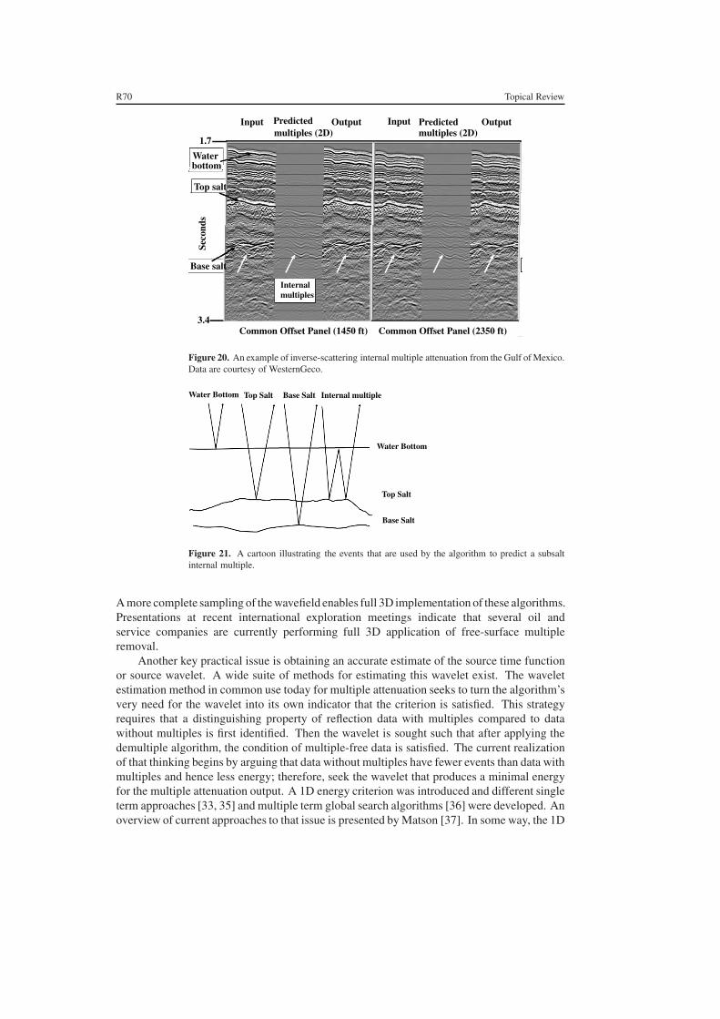
R70 Topical Review
Input Predictedmultiples (2D)
Output Input Predictedmultiples (2D)
Output
1.7
Waterbottom
Top salt
Seco
nds
Base salt
3.4Common Offset Panel (1450 ft) Common Offset Panel (2350 ft)
Internalmultiples
Figure 20. An example of inverse-scattering internal multiple attenuation from the Gulf of Mexico.Data are courtesy of WesternGeco.
Water Bottom Top Salt Base Salt Internal multiple
Water Bottom
Top Salt
Base Salt
Figure 21. A cartoon illustrating the events that are used by the algorithm to predict a subsaltinternal multiple.
A more complete sampling of the wavefield enables full 3D implementation of these algorithms.Presentations at recent international exploration meetings indicate that several oil andservice companies are currently performing full 3D application of free-surface multipleremoval.
Another key practical issue is obtaining an accurate estimate of the source time functionor source wavelet. A wide suite of methods for estimating this wavelet exist. The waveletestimation method in common use today for multiple attenuation seeks to turn the algorithm’svery need for the wavelet into its own indicator that the criterion is satisfied. This strategyrequires that a distinguishing property of reflection data with multiples compared to datawithout multiples is first identified. Then the wavelet is sought such that after applying thedemultiple algorithm, the condition of multiple-free data is satisfied. The current realizationof that thinking begins by arguing that data without multiples have fewer events than data withmultiples and hence less energy; therefore, seek the wavelet that produces a minimal energyfor the multiple attenuation output. A 1D energy criterion was introduced and different singleterm approaches [33, 35] and multiple term global search algorithms [36] were developed. Anoverview of current approaches to that issue is presented by Matson [37]. In some way, the 1D
Topical Review R71
energy minimization methods for finding the wavelet represent a weak link in how free-surfaceand internal multiple attenuation is applied in practice. The methods for finding the waveletare not as physically complete (and effective) as the multiple removal methods that they aremeant to serve. For example, the free-surface and internal multiple attenuation methods haveno problem with interfering events; but the removal of a multiple proximal to and destructivelyinterfering with a primary could cause the energy to rise (rather than fall) with the removal ofthe multiple. New methods (e.g., [38–41]) are being developed for predicting the wavelet thatare as complete as, and on a conceptual and effectiveness par with, the inverse series multipleattenuation procedures that they are meant to serve.
Often the series is truncated to only a single multiple prediction term and an adaptivewavelet estimation scheme is used to adaptively subtract the internal multiples from the inputdata. For internal multiples, numerical tests indicate that it is more difficult to estimate thewavelet post-internal multiple prediction. This is due to the fact that the 1D minimum energycriterion is often invalid and too blunt an instrument for the subtlety of internal multiplesand complex free-surface multiples. Fortunately, the two processes require the same wavelet;thus the wavelet estimated for the free-surface multiple attenuation step will often suffice forinternal multiple attenuation, as was the case in the field data example shown here. Currently,compromises made with truncated series algorithms, too great a dependence on adaptiveparameters and less than adequate measurement coverage are all inhibiting the full power ofthese methods from being realized. With multi-term series applications, improved predictedwavelets and a full 3D point receiver acquisition, we anticipate that the inverse scatteringdemultiple methods will reach their full practical potential.
7.5. Inverse scattering series and the feedback methods for attenuating multiples
Removing multiples from seismic reflection data is a long-standing problem that hasexperienced significant progress over the past ten years, but still has open issues to address.An overview of the landscape of techniques can be found in [42] and several collaborativeworks with members of the Delphi group (e.g., [43, 44]). Berkhout, Verschuur and theDelphi group developed a free-surface and interface feedback procedure for describing free-surface multiples and primaries and internal multiples and also for attenuating free-surfaceand internal multiples, respectively. The inverse scattering approach uses the free surface forfree-surface multiples and a point-scatterer model for primaries and internal multiples. Theinverse-scattering free surface demultiple method is conceptually complete, whereas the free-surface feedback approach represents certain compromises that involve the obliquity factorand source deghosting that place an added burden on the adaptive wavelet, especially at largedistances from the source along the receiver line. The feedback method provides an effectiveand efficient method for attenuating internal multiples when the reflector that generates thedownward reflection can be isolated. The inverse scattering series approach provides themost comprehensive method for attenuating all free-surface and internal multiples with nosubsurface information whatsoever and no event picking, velocity analysis or interpretiveintervention.
The inverse scattering series methods provide significant added value when the subsurfaceis complex, when reflectors are dipping, corrugated or diffractive, when events are subtle andpartly coincident in time and when the interest is in removing all internal multiples. Issues thatinvolve the practical prerequisites of these series solutions are all important and methods forsatisfying those prerequisites include source signature estimation, areal coverage of surfacemeasurements and deghosting. Considerable resources are currently devoted to addressingand improving the satisfaction of these prerequisites.
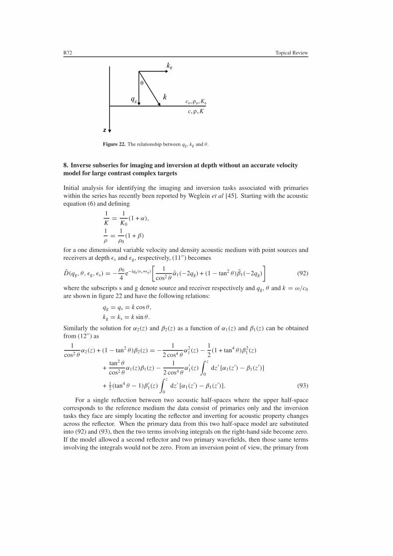
R72 Topical Review
Figure 22. The relationship between qg, kg and θ .
8. Inverse subseries for imaging and inversion at depth without an accurate velocitymodel for large contrast complex targets
Initial analysis for identifying the imaging and inversion tasks associated with primarieswithin the series has recently been reported by Weglein et al [45]. Starting with the acousticequation (6) and defining
1
K= 1
K0(1 + α),
1
ρ= 1
ρ0(1 + β)
for a one dimensional variable velocity and density acoustic medium with point sources andreceivers at depth εs and εg, respectively, (11′′) becomes
D(qg, θ, εg, εs) = −ρ0
4e−iqg(εs+εg)
[1
cos2 θα1(−2qg) + (1 − tan2 θ)β1(−2qg)
](92)
where the subscripts s and g denote source and receiver respectively and qg, θ and k = ω/c0
are shown in figure 22 and have the following relations:
qg = qs = k cos θ,
kg = ks = k sin θ.
Similarly the solution for α2(z) and β2(z) as a function of α1(z) and β1(z) can be obtainedfrom (12′′) as
1
cos2 θα2(z) + (1 − tan2 θ)β2(z) = − 1
2 cos4 θα2
1(z) − 1
2(1 + tan4 θ)β2
1 (z)
+tan2 θ
cos2 θα1(z)β1(z) − 1
2 cos4 θα′
1(z)∫ z
0dz′ [α1(z
′) − β1(z′)]
+ 12 (tan4 θ − 1)β ′
1(z)∫ z
0dz′ [α1(z
′) − β1(z′)]. (93)
For a single reflection between two acoustic half-spaces where the upper half-spacecorresponds to the reference medium the data consist of primaries only and the inversiontasks they face are simply locating the reflector and inverting for acoustic property changesacross the reflector. When the primary data from this two half-space model are substitutedinto (92) and (93), then the two terms involving integrals on the right-hand side become zero.If the model allowed a second reflector and two primary wavefields, then those same termsinvolving the integrals would not be zero. From an inversion point of view, the primary from
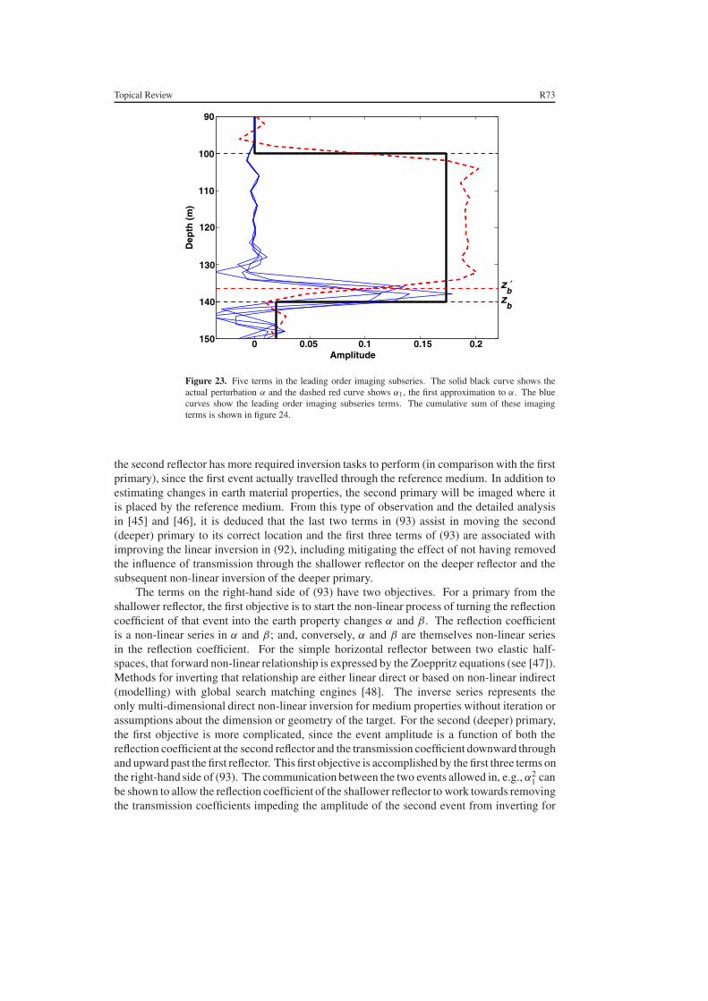
Topical Review R73
′
Figure 23. Five terms in the leading order imaging subseries. The solid black curve shows theactual perturbation α and the dashed red curve shows α1, the first approximation to α. The bluecurves show the leading order imaging subseries terms. The cumulative sum of these imagingterms is shown in figure 24.
the second reflector has more required inversion tasks to perform (in comparison with the firstprimary), since the first event actually travelled through the reference medium. In addition toestimating changes in earth material properties, the second primary will be imaged where itis placed by the reference medium. From this type of observation and the detailed analysisin [45] and [46], it is deduced that the last two terms in (93) assist in moving the second(deeper) primary to its correct location and the first three terms of (93) are associated withimproving the linear inversion in (92), including mitigating the effect of not having removedthe influence of transmission through the shallower reflector on the deeper reflector and thesubsequent non-linear inversion of the deeper primary.
The terms on the right-hand side of (93) have two objectives. For a primary from theshallower reflector, the first objective is to start the non-linear process of turning the reflectioncoefficient of that event into the earth property changes α and β. The reflection coefficientis a non-linear series in α and β; and, conversely, α and β are themselves non-linear seriesin the reflection coefficient. For the simple horizontal reflector between two elastic half-spaces, that forward non-linear relationship is expressed by the Zoeppritz equations (see [47]).Methods for inverting that relationship are either linear direct or based on non-linear indirect(modelling) with global search matching engines [48]. The inverse series represents theonly multi-dimensional direct non-linear inversion for medium properties without iteration orassumptions about the dimension or geometry of the target. For the second (deeper) primary,the first objective is more complicated, since the event amplitude is a function of both thereflection coefficient at the second reflector and the transmission coefficient downward throughand upward past the first reflector. This first objective is accomplished by the first three terms onthe right-hand side of (93). The communication between the two events allowed in, e.g., α2
1 canbe shown to allow the reflection coefficient of the shallower reflector to work towards removingthe transmission coefficients impeding the amplitude of the second event from inverting for

R74 Topical Review
′
Figure 24. The cumulative sum of five terms in the leading order imaging subseries. The solidblack curve shows the perturbation α and the red curve shows the first approximation to α or the firstterm in the inverse series, α1. The blue curve shows the cumulative sum of the imaging subseriesterms; e.g. in panel (ii) the sum of two terms in the subseries is shown and in panel (v) the sum offive terms in the subseries is displayed.
Figure 25. A one dimensional acoustic model.
local properties at the second reflector. Hence, specific communications between primariesfrom different reflectors work together to remove the extraneous transmission coefficients ondeeper primaries that are suffering from being given the wrong imaging velocity.
Similarly, the integral terms on the right-hand side of (93) represent a recognition that thereference velocity will give an erroneous image and asks for an integral of α1 − β1, the linearapproximation to the change in acoustic velocity, from the onset of α1 − β1 down to the depth

Topical Review R75
F i g u
r e
2 6 .
α1d i s p l a y e d a s a f u n c t i o n o f t w o a n g l e s . T
h e g r a p h o n t h e r i g h t i s a c o n t o u r p l o t o ft h e g r a p h o n t h e l e f t . I n t h i s e x a m p l e , t h e e x a c t v a l u e o f α
i s 0 . 2 9 2 5
Figure 27. The sum
α
1
+
α
2
displayed as a function of two angles for the same example as infigure 26 where the exact value of
α is 0.292.
needing the imaging help. Two important observations. (1) When the actual velocity does notchange across an interface, R
(θ) is not a function of
θ and from (92) it can be shown that
α
1
−
β
1
=
(
�V
V
)
1
=
0
.
Therefore, when the actual velocity does not change then the linear approximation to the changein velocity is zero. Therefore, wh
en the velocity is equal to the reference across all reflectors
(e.g., when density changes but not velocity) then these equations do not correct the locationwhere the reference velocity lo
cates those events, which in that case is correct. (2) The errorin locating reflectors caused by an error in velocity depends on both the size of the error andthe duration of the error. Hence, the integral of α
1
−
β
1
represents an amplitude and durationcorrection to the originally mislocated primary. A gen
eral principle is that when an inversiontask has a duration aspect for the problem being addressed, the response has an integral overa measure of that error in the solution. The inverse series empowers the primary events in thedata to ‘speak to themselves’ for non-linear inversion and to ‘speak to each other’ to deal with
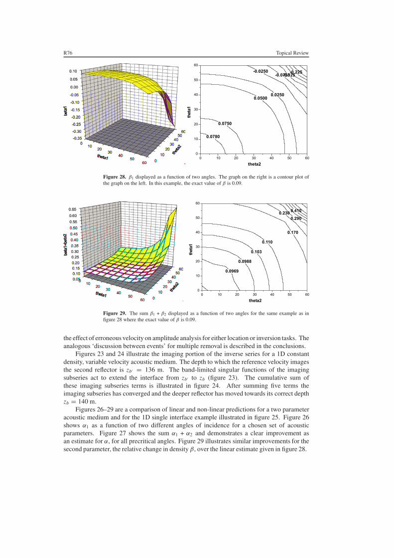
R76 Topical Review
Figure 28. β1 displayed as a function of two angles. The graph on the right is a contour plot ofthe graph on the left. In this example, the exact value of β is 0.09.
Figure 29. The sum β1 + β2 displayed as a function of two angles for the same example as infigure 28 where the exact value of β is 0.09.
the effect of erroneous velocity on amplitude analysis for either location or inversion tasks. Theanalogous ‘discussion between events’ for multiple removal is described in the conclusions.
Figures 23 and 24 illustrate the imaging portion of the inverse series for a 1D constantdensity, variable velocity acoustic medium. The depth to which the reference velocity imagesthe second reflector is zb′ = 136 m. The band-limited singular functions of the imagingsubseries act to extend the interface from zb′ to zb (figure 23). The cumulative sum ofthese imaging subseries terms is illustrated in figure 24. After summing five terms theimaging subseries has converged and the deeper reflector has moved towards its correct depthzb = 140 m.
Figures 26–29 are a comparison of linear and non-linear predictions for a two parameteracoustic medium and for the 1D single interface example illustrated in figure 25. Figure 26shows α1 as a function of two different angles of incidence for a chosen set of acousticparameters. Figure 27 shows the sum α1 + α2 and demonstrates a clear improvement asan estimate for α, for all precritical angles. Figure 29 illustrates similar improvements for thesecond parameter, the relative change in density β, over the linear estimate given in figure 28.

Topical Review R77
Table 1. Summary of task-specific subseries.
Task Properties
Free-surface mul-tiple elimination
One term in the subseries predicts precisely the time and amplitude ofall free-surface multiples of a given order independently of the rest ofthe history of the event. Order is defined as number of times the multiplehas a downward reflection at the free surface.
Internal multipleattenuation
One term in the inverse series predicts the precise time and approximateamplitude of all internal multiples of a given order. The order of aninternal multiple is defined by the number of downward reflections fromany subsurface reflector at any depth.
Imaging at depthwithout the accu-rate velocity
The first term in the series corresponds to current migration or migration-inversion. To achieve a well-estimated depth map requires further termsin the imaging subseries directly in terms of an inaccurate velocity model.A priori velocity estimation will aid the rate of convergence.
Inversion at depthwithout the exactoverburden
The first term in the subseries corresponds to current linear amplitudeanalysis. Improvement to linear estimates of earth property changesand accounting for inadequate overburden requires further terms in theseries. Tests indicate rapid convergence for the first non-linear parameterestimation objective.
Early analysis and tests are encouraging and demonstrate the intrinsic potential for thetask-specific inverse subseries to perform imaging at the correct depth [49] and improving uponlinear estimation of earth material properties [50], without the need for an accurate velocitymodel. Furthermore, numerical tests indicate: (1) that the imaging subseries converges forvelocity errors that are large in amplitude and duration; and (2) rapid improvement in estimatesof earth material properties beyond the current industry standard linear amplitude analysis.
9. Conclusions and summary
We have described the historical development and a methodology for deriving direct multi-dimensional non-linear seismic data processing methods from the inverse scattering series.To date, the inverse scattering series have yielded subseries for free-surface and internalmultiple attenuation, imaging primaries at depth and inverting for earth material properties.The hallmark of these methods is their ability to achieve their objective directly in terms ofincomplete or inaccurate a priori subsurface information and without ever iterating or updatingthat input or assuming that it is proximal to actual properties.
The development features an interplay between an understanding of the forward scatteringprocess and task separation in the inverse scattering series. The forward series begins withthe reference propagator, G0, and the perturbation operator, V(r, ω), the difference betweenactual and reference medium properties as a function of space, r, and frequency ω. The inverseseries inputs data, D(rg, rs, t), a function of time and the reference propagator, G0.
Since the forward series inputs the perturbation, V(r, ω), and rapid variation of Vcorresponds to the exact spatial location of reflectors, it follows that space is the domainof comfort of the forward series. In contrast, the computation of the time of arrival of any (andevery) seismic event for which the actual medium propagation is not described by G0 requiresan infinite series to obtain the correct time from the forward series. In this respect, time is thedomain of discomfort for the forward series for seismic events.

R78 Topical Review
For the inverse series, the input is data in time D(rg, rs, t) and processes that involvetransforming D(rg, rs, t) to another function of time, e.g., the data without free-surfacemultiples D′(rg, rs, t), are simpler to achieve than tasks such as imaging primaries in spacethat require a map from time to space (i.e., D(rg, rs, t) to V(r, ω)). Hence, time is the domainof comfort for the inverse series. Emphasizing this point, the correct time (and amplitude) forconstructing any internal multiple requires an infinite number of terms in the forward serieswhereas the prediction of the precise time and well-approximated amplitude for every internalmultiple occurs in the first term of the inverse (removal) subseries for that order of multiple,totally independently of the depths of the reflectors that generate the multiple.
In addition, if accurate a priori information can be provided for the localization andseparation of a given task where the task is defined in terms of separating events that have awell-defined experience from those events that have not, then further efficiency can derive fromsubseries that involve time to time maps, for example, in the case where a free-surface reflectioncoefficient (or GFS
0 ) is supplied for the task of removing the ghosts and free-surface multiples.In the latter case, one term in the free-surface multiple removal subseries precisely predictsthe time and amplitude of all multiples of that order. In table 1, we summarize the amountof effort required to achieve a certain level of effectiveness for each of the four task-specificsubseries.
The strategy is to accomplish one task at a time, in the order listed, and then restartthe problem as though the just completed task never existed. This is advantageous inthat it avoids the terms associated with coupled tasks in the inverse series. Furthermore,carrying these tasks out in sequence can enhance the ability of subsequent tasks to reachtheir objective. For example, the free-surface and internal multiple algorithms do not require(or benefit from) accurate a priori information. However, the removal of free-surface andinternal multiples significantly improves our ability to estimate the overburden velocity modeland subsequently aids the efficacy and efficiency of the imaging and inversion subseries forprimaries.
Since the rate of convergence, for both multiple removal subseries, does not benefit fromanything closer to the earth than water speed and the costs of the algorithms quickly increasewith complexity of the reference medium, the idea is to perform these tasks with efficient,constant water velocity reference propagation.
In tackling the next step, the approach is to restart the problem assuming that certaindata issues have already been addressed. For example, after free-surface and internal multipleremoval, we restart the problem assuming a primary-only data set resulting in an inverse seriesthat requires proximal velocity information and consequently more complex and more costlysubseries for tasks that benefit from that additional information.
If you do not like the strategy of ‘isolate a task and then restart the problem’ and youwant to be a purist and start and end with one inverse scattering series, then you would needa single complex reference medium that would allow the toughest task to have an opportunityto succeed. There are two issues with the latter approach:
(1) the proximal velocity can be difficult to obtain when troublesome multiples are in yourinput data; and
(2) the single all-encompassing series is an ‘all or nothing’ strategy that does not allow forstages to succeed and provide benefit when the overall series or its more ambitious goalsare beyond reach.
Although both primaries and multiples have experienced the subsurface and, hence, carryinformation encoded in their character, the indisputable attitude or orientation of the inverse

Topical Review R79
scattering series (the only currently known multi-dimensional direct inversion method foracoustic and elastic media) is to treat multiples as coherent noise to be removed and treatprimaries as the provider of subsurface information. That does not mean that one couldnever use multiples in some inclusive rather than exclusive method that seeks to exploit theinformation that both primaries and multiples contain. It simply means that an inclusive theory,starting with realistic a priori information, does not currently exist and, further, that the inverseseries definitely and unambiguously adopts the exclusive view: multiples are considered noisethat it removes while primaries are the signal with useful subsurface information.
While it certainly follows from the mathematics of (11)–(14) that it is possible to directlyachieve seemingly impossible inversion objectives from data with only a reference mediumpropagator that is assumed to be not equal to G and hence inadequate, there is also valuein providing an understanding from an information content point of view (see also [5]).What basically happens in each task-specific subseries is that specific conversations take placebetween events in the data as a whole that allow, e.g., multiple prediction or accurate depthimaging to take place without an accurate velocity model. ‘Non-linear in the data’ is the keyand means that quadratic terms enter the picture (data times data, at least) and that allowsdifferent events to have multiplicative communication.
For example, if you provide the medium in detail you can readily determine throughmodelling whether any event in the data is a primary or multiple. However, if you provideonly an isolated event, without the medium properties, then there is no way to determinewhether it is a primary or multiple; in fact it can be either for different models. So how doesthe inverse series work out whether the event is a primary or multiple without any subsurfaceinformation? Since it is a series, there is a ‘conversation’ set up with other events and then ayes or no as to whether an event is a primary or multiple is completely achievable without anyinformation about the medium.
In the subseries for imaging at depth without an accurate velocity, the first term is thecurrent state-of-the-art migration with your best estimated velocity model and places eachevent exactly where that input reference velocity dictates. All current imaging methods arelinear in the data, and once the velocity model is chosen, the collection of all primaries (fromall reflectors) as a whole are not asked their ‘view’ or ‘opinion’ of the input velocity nor arethey allowed to ‘discuss’ it amongst themselves.
The second term in the inverse series, e.g. (93), has integral terms that start to movethe incorrectly imaged events resulting from the linear migration step towards their correctlocation. There is a quadratic dependence on the data, allowing multiplicative conversationsbetween primary events from two different reflectors, and they are empowered to have anopinion about the input velocity. If they decide together that (at least) one of the events hasbeen provided with a velocity model that is inconsistent with those two events, then the troubledevent (usually deeper) asks for assistance from a shallower event to help it use its amplitude,and the difference of their arrival times, to move the deeper primary towards its correct location.Furthermore, and perhaps most important, when the first term beyond current best practiceis computed, the quadratic term immediately and unambiguously judges the adequacy of theinput velocity. If the result of the first non-linear conversation between primaries (representedby the terms with integrals in the imaging series) is a determination that the velocity is adequate,then the imaging series stops, and returns a zero value for the correction to spatial locationsending the message that the data all together judge the velocity as adequate and to proceedwith current linear migration for locating reflectors in space. There is no mindless (and costly)perturbation about no change in depth—rather a clear signal to stop the imaging series. This isanother important example of purposeful perturbation. The term containing
∫(α1 − β1)dz in
(93) exists to correct depth imaging for incorrect input velocity, but first determines whether
R80 Topical Review
its function is required by a conversation between all the primaries about the adequacy of thevelocity expressed through α1 − β1. As we explained, α1 − β1 will be computed as zero whenthe velocity is adequate.
When the velocity is determined to be adequate, the inversion subseries that predictschanges in earth material properties will provide added value beyond current industry practicefor arbitrary geometry of target and small or large changes in elastic properties and densityacross the target. When the velocity is determined to be inadequate, those same non-linearinversion objectives are achieved directly in terms of the inadequate velocity model. Hence,the inverse series and the task-specific subseries represent a fundamentally new capabity forimaging and inverting primaries, as they had earlier provided for the removal of multiples.
In progressing from migration to migration-inversion [3, 32] one addressed not just wherethe reflector is located in space but also what material properties changed across that imagedreflector. One issue in making that step is the need to consider both the amplitude as well asthe phase of the back-propagating wave in the estimated reference medium. When the abilityto estimate the reference medium is far from adequate and migration-inversion is performedin the reference medium as a first step in the imaging subseries, then the bar on the migration-inversion is higher still (in comparison to migration-inversion when the reference is adequateand the latter is the final product) requiring a need for fidelity on phase, amplitude and spectralcontent. The imaging subseries expects the complete and correct migration-inversion in theincorrect medium. Since the relationships between variables and their Fourier conjugatesare markedly different in, e.g., wave, coherent state and asymptotic migration techniques, wewould expect a preference for wave theory migration and an appropriate sampling and coverageof surface recording that preserves, e.g., all kg components in a given xg.
Serious conceptual and practical hurdles in the theoretical evolution, algorithmdevelopment and robust industrial application had to be overcome to bring the inverse scatteringmultiple attenuation subseries methods to their current state of efficacy. We anticipate that inbringing the subseries for imaging and inverting primaries through that same process, stillhigher hurdles and tougher prerequisites will be addressed. This new vision of processingsignal in seismic data has game-changing potential for the exploration and production ofhydrocarbons. We would also anticipate that these inverse scattering series methods and thenew methods for satisfying their prerequisites (e.g., source signal identification) might serve toencourage other fields of non-destructive evaluation to benefit from these efforts—fields such asmedical imaging, environmental monitoring, nuclear, atomic and molecular identification andsignal enhancement, military and defence detection, identification and guidance applicationsand global and crustal seismology.
Acknowledgments
Craig Cooper, Jon Sheiman, Robert Keys, Michael Bostock, Roel Snieder, Kris Innanen, Fonsten Kroode, Tadeusz Ulrych and Ken Larner are thanked for useful and constructive commentsand suggestions. The support of the M-OSRP sponsors is gratefully acknowledged. The TexasAdvanced Research Program (ARP # 003652-0624-2001) is acknowledged for partial supportof this research.
References
[1] Cohen J K and Bleistein N 1977 An inverse method for determining small variations in propagation speed SIAMJ. Appl. Math. 32 784–99
[2] Morley L and Claerbout J 1983 Predictive deconvolution in shot-receiver space Geophysics 48 515–31[3] Stolt R H and Weglein A B 1985 Migration and inversion of seismic data Geophysics 50 2458–72
Topical Review R81
[4] Weglein A B, Boyse W E and Anderson J E 1981 Obtaining three-dimensional velocity information directlyfrom reflection seismic data: an inverse scattering formalism Geophys ics 46 1116–20
[5] Weglein A B, Gasparotto F A, Carvalho P M and Stolt R H 1997 An inverse scattering series method forattenuating multiples in seismic reflection data Geophysics 62 1975–89
[6] Newton R G 2002 Scattering Theory of Waves and Particles (New York: Dover)[7] Taylor J R 1972 Scattering Theory (New York: Wiley)[8] Clayton R W and Stolt R H 1981 A Born–WKBJ inversion method for acoustic reflection data Geophys. Soc.
Explor. Geophys. 46 1559–67[9] Matson K H 1997 An inverse-scattering series method for attenuating elastic multiples from multicomponent
land and ocean bottom seismic data PhD Thesis University of British Columbia[10] Moses H E 1956 Calculation of scattering potential from reflection coefficients Phys. Rev. 102 559–67[11] Prosser R T 1969 Formal solutions of inverse scattering problems J. Math. Phys. 10 1819–22[12] Razavy M 1975 Determination of the wave velocity in an inhomogeneous medium from reflection data J. Acoust.
Soc. Am. 58 956–63[13] Stolt R H and Jacobs B 1980 Inversion of seismic data in a laterally heterogeneous medium SEP Rep. 24 135–52[14] Carvalho P M 1992 Free-surface multiple reflection elimination method based on nonlinear inversion of seismic
data PhD Thesis Universidade Federal da Bahia, Brazil (in Portuguese)[15] ten Kroode F 2002 Prediction of internal multiples Wa v e M o tion 35 315–38[16] Weglein A B and Matson K 1998 Inverse-scattering interval multiple attenuation: an analytic example
and subevent interpretation Mathematical Methods in Geophysical Imaging (Proc. SPIE vol 3453) edS Hassanzadeh (Bellingham, WA: SPIE) pp 1008–17
[17] Coates R T and Weglein A B 1996 Internal multiple attenuation using inverse scattering: results from prestack1 and 2D acoustic and elastic synthetics 66th Ann. Int. SEG Mtg pp 1522–5 (expanded abstracts)
[18] Matson K 1996 The relationship between scattering theory and the primaries and multiples of reflection seismicdata J. Seism. Explor. 5 63–78
[19] Nita B, Matson K and Weglein A B 2003 Forward scattering series seismic events: far-field approximations,critical and postcritical reflections SIAM J. Appl. Math. submitted
[20] Innanen K A and Weglein A B 2003 Viscoacoustic Born Series Continued: Toward Scattering-Based QCompensation/Estimation in preparation
[21] Keys R G and Weglein A B 1983 Generalized linear inversion and the first Born theory for acoustic mediaJ. M a t h . P h y s . 24 1444–9
[22] Devaney A J and Weglein A B 1989 Inverse scattering using the Heitler equation Inverse Problems5 L49–52
[23] Weglein A B, Matson K H, Foster D J, Carvalho P M, Corrigan D and Shaw S A 2000 Imaging and inversionat depth without a velocity model 70th Ann. Int. SEG Mtg (Calgary, Alberta, 2000)
[24] Boyse W E 1986 Wave Propagation and Inversion in Slightly Inhomogeneous Media p 40[25] Boyse W E and Keller J B 1986 Inverse elastic scattering in three dimensions J. Acoust. Soc. Am. 79 215–8[26] Ware J A and Aki K 1969 Continuous and discrete inverse-scattering problems in a stratified elastic medium. I.
Plane waves at normal incidence J. Acoust. Soc. Am. 45 911–21[27] Fokkema J T and van den Berg P M 1993 Seismic Applications of Acoustic Reciprocity (Amsterdam: Elsevier)[28] Berkhout A J 1982 Seismic Migration, Imaging of Acoustic Wave energy by Wavefield Extrapolation, A:
Theoretical Aspects 2nd edn (Amsterdam: Elsevier)[29] Araujo F V 1994 Linear and nonlinear methods derived from scattering theory: backscattered tomography and
internal multiple attenuation PhD Thesis Universidade Federal da Bahia, Brazil (in Portuguese)[30] Araujo F V, Weglein A B, Carvalho P M and Stolt R H 1994 Internal multiple attenuation 56th Meeting of
Association of Exploration Geophysicists, session H036[31] Araujo F V, Weglein A B, Carvalho P M and Stolt R H 1994 Inverse scattering series for multiple attenuation:
an example with surface and internal multiples 64th Ann. Int. SEG Mtg pp 1039–41 (expanded abstracts)[32] Weglein A B and Stolt R H 1999 Migration-inversion revisited Leading Edge 18 950–2[33] Ikelle L T, Roberts G and Weglein A B 1995 Source signature estimation based on the removal of first order
multiples 65th Ann. Int. SEG Mtg pp 1478–81 (expanded abstracts)[34] Verschuur D J, Berkhout A J and Wapenaar C P A 1992 Adaptative surface-related multiple elimination
Geophysics 57 1166–77[35] Verschuur D J and Berkhout A J 1992 Surface-related multiple elimination and wavelet estimation 54th EAEG
Mtg vol 7, pp 568–9[36] Carvalho P M and Weglein A B 1994 Wavelet estimation for surface multiple attenuation using a simulated
annealing algorithm 64th Ann. Int. SEG Mtg (Los Angeles, CA, 1994) (expanded abstracts)
R82 Topical Review
[37] Matson K H 2000 An overview of wavelet estimation using free-surface multiple removal Leading Edge 1950–5
[38] Weglein A B and Secrest B G 1990 Wavelet estimation from marine pressure measurements Geophysics 632108–19
[39] Osen A, Secrest B G, Amundsen L and Reitan A 1998 Wavelet estimation from marine pressure measurementsGeophysics 63 2108–19
[40] Tan T H 1999 Wavelet spectrum estimation Geophysics 64 1836–46[41] Weglein A B, Tan T H, Shaw S A, Matson K H and Foster D J 2000 Prediction of the wavefield anywhere above
an ordinary towed streamer 70th Ann. Int. SEG Mtg (Calgary, Alberta, 2000)[42] Weglein A B 1999 Multiple attenuation: an overview of recent advances and the road ahead Leading Edge 18
40–4[43] Berkhout A J, Verschuur D J and Weglein A B 2000 Wave theoretic multiple attenuation: part I Conf. on Offshore
Technology (Houston, TX, 2000)[44] Weglein A B, Matson K H and Berkhout A J 2000 Wave theoretic multiple attenuation: part II Conf. on Offshore
Technology (Houston, TX, 2000)[45] Weglein A B, Foster D J, Matson K H, Shaw S A, Carvalho P M and Corrigan D 2002 Predicting the correct
spatial location of reflectors without knowing or determining the precise medium and wave velocity: initialconcept, algorithm and analytic and numerical example J. Seism. Explor. 10 367–82
[46] Shaw S A and Weglein A B 2003 Imaging seismic reflection data at the correct depth without specifying anaccurate velocity model: initial numerical examples of an inverse scattering subseries Frontiers of RemoteSensing Information Processing ed C H Chen (Singapore: World Scientific)
[47] Aki K and Richards P G 2002 Quantitative Seismology 2nd edn (Mill Valley, CA: University Science Books)p 704
[48] Sen M and Stoffa P L 1995 Global Optimization Methods in Geophysical Inversion (Amsterdam: Elsevier)p 294
[49] Shaw S A, Weglein A B, Foster D J, Matson K H and Keys R G 2003 Isolation of a leading order depth imagingseries and analysis of its convergence properties, in preparation
[50] Zhang H and Weglein A B 2003 Target identification using the inverse scattering series; inversion of large-contrast, variable velocity and density acoustic media, in preparation
Further reading
Amundsen L 2001 Elimination of free-surface related multiples without need of the source wavelet Geophysics 66327–41
Carvalho P M, Weglein A B and Stolt R H 1991 Examples of a nonlinear inversion method based on the T matrix ofscattering theory: application on multiple suppression 61st Ann. Int. SEG Mtg pp 1319–22 (expanded abstracts)
Carvalho P M, Weglein A B and Stolt R H 1992 Nonlinear inverse scattering for multiple suppression: applicationto real data: part I 62nd Ann. Int. SEG Mtg pp 1093–5 (expanded abstracts)
Devaney A J 1989 Structure determination from intensity measurements in scattering experiments Phys. Rev. Lett.62 2385–8
Dragoset W H 1992 Surface multiple attenuation—theory, practical issues, examples EAEG Abstracts BO27Ikelle L T and Weglein A B 1996 Attenuation of free-surface multiples in multi-offset VSP data J. Seism. Explor. 5
363–78Kennett B L N 1979 The suppression of surface multiples on seismic records Geophys. Prospect. 27 484–600Manin M and Spitz S 1995 3D attenuation of targeted multiples with a pattern recognition technique 57th EAEG
Conf. (Glasgow) BO46 (expanded abstracts)Matson K H, Paschal D and Weglein A B 1999 A comparison of three multiple attenuation methods applied to a hard
water-bottom data set Leading Edge 18 120–6Matson K and Weglein A B 1996 Free-surface elastic multiple removal using inverse scattering Canadian SEG
(expanded abstracts)Matson K H and Weglein A B 1996 Removal of elastic interface multiples from land and ocean bottom data using
inverse scattering 66th Ann. Int. SEG Mtg (Denver, CO, 1996) pp 1526–9 (expanded abstracts)Newton R G 1981 Inversion of reflection data for layered media: a review of exact methods Geophys. J. R. Astron.
Soc. 65 191–215Riley D C and Claerbout J F 1976 2D multiple reflections Geophysics 41 592–620Snieder R 1990 The role of the Born approximation in nonlinear inversion Inverse Problems 6 247–66Snieder R 1991 An extension of Backus–Gilbert theory to nonlinear inverse problems Inverse Problems 7 409–33Stolt R H and Jacobs B 1981 An approach to the inverse seismic problem SEP Rep. 25 121–32

Topical Review R83
Weglein A B 1985 The inverse scattering concept and its seismic application Developments in Geophysical ExplorationMethods vol 6, ed A A Fitch (Amsterdam: Elsevier) pp 111–38
Weglein A B 1995 Multiple attenuation: recent advances and the road ahead 65th Ann. Int. SEG Mtg pp 1492–5(expanded abstracts)
Wolf E 1969 Three dimensional structure determination of semi-transparent objects from holographic data Opt.Commun. 1 153