Embed Size (px)
Citation preview
http://www.gsd.uab.cat
INVERSE PROBLEMS IN DARBOUX’ THEORY OF INTEGRABILITY
COLIN CHRISTOPHER1, JAUME LLIBRE2, CHARA PANTAZI3 AND SEBASTIAN WALCHER4
Abstract. The Darboux theory of integrability for planar polynomial differential equationsis a classical field, with connections to Lie symmetries, differential algebra and other areasof mathematics. In the present paper we introduce the concepts, problems and inverseproblems, and we outline some recent results on inverse problems. We also prove a newresult, viz. a general finiteness theorem for the case of prescribed integrating factors. Anumber of relevant examples and applications is included.
1. Introduction and preliminaries
Consider a planar complex polynomial vector field
X = P∂
∂x+Q
∂
∂y, (1)
and the associated ordinary differential equation
x = P (x, y),y = Q(x, y).
(2)
There is a simple approach, initiated by Darboux [15] in 1878, to construct first integralsand integrating factors for polynomial equations (2) which admit sufficiently many invariantalgebraic curves. An account of this is contained in the classical monograph by Ince [16],Ch. II, Section 2.2. Jouanolou [17] extended this method to obtain criteria for the existenceof rational first integrals. Darboux’ theory of integrability for planar polynomial vector fieldswas developed further in recent years, see for instance [8, 9, 6, 5]. An inverse problemgenerally consists in determining all differential equations satisfying some given properties,such as admitting a given integrating factor.
Given irreducible pairwise relatively prime polynomials f1, . . . , fr and nonzero complexconstants d1, . . . , dr, one says that X (or equation (2)) admits the Darboux integrating factor
f−d11 · · · f−dr
r , (3)
if
div(f−d11 · · · f−dr
r X)= 0. (4)
Recall that divergence zero characterizes vector fields with volume-preserving local flow.In dimension two a local first integral of a divergence zero vector field can be determinedexplicitly by quadratures. Of course one knows that, due to the straightening theorem (or tostandard existence theorems for quasi-linear partial differential equations), the local existence
J. Llibre and C. Pantazi are partially supported by the MICIIN/FEDER grant MTM2008–03437. JLis additionally partially supported by a CIRIT grant number 2009SGR410 and by ICREA Academia. CP isadditionally partial supported by the MICIIN/FEDER grant number MTM2009-06973 and by the Generalitatde Catalunya grant number 2009SGR859. S. Walcher acknowledges the hospitality and support of the CRMand the Mathematics Department at UAB during visits when this manuscript was prepared.
1
This is a preprint of: “Inverse problems in Darboux’ theory of integrability”, Colin J. Christopher,Jaume Llibre, Chara Pantazi, Sebastian Walcher, Acta Appl. Math., vol. 120, 101–126, 2012.DOI: [10.1007/s10440-012-9671-9]
2 C. CHRISTOPHER, J. LLIBRE, C. PANTAZI AND S. WALCHER
of first integrals or integrating factors near a non-stationary point is guaranteed. But ourinterest lies in constructive approaches.
Necessary for the existence of a Darboux integrating factor is the invariance of all complexzero sets Ci of fi for X, thus every Ci is an invariant set for equation (2). Equivalently, dueto Hilbert’s Nullstellensatz, there exist polynomials L1, . . . , Lr such that
Xfi = Li · fi, 1 ≤ i ≤ r. (5)
fi is then called a semi-invariant of X, with cofactor Li, and one also says that X admits fi.With f := f1 · · · fr the latter set of conditions is also equivalent to
Xf = (L1 + · · ·+ Lr) · f.Given invariance, X admits the Darboux integrating factor (3) if and only if
d1 · L1 + · · ·+ dr · Lr = divX. (6)
We refer to [26], [13] and [11] for more details and proofs. All these concepts and results arealso applicable to real polynomial (or analytic) systems, via complexification, and complexinvariant curves and integrating factors are relevant for the analysis of real systems.
Why is there interest in these topics? First of all, they are classical, going back to Poincareand Darboux. Moreover, there is a correspondence between integrating factors and Lie sym-metries of first-order equations (see Olver [19]). Lie symmetries of such equations are notalgorithmically accessible although (or rather, because) they abound, and therefore one seeksfor approaches which avoid invoking the non-constructive straightening theorem. Integrat-ing factors from a restricted class of functions (such as given in (3)) open a possible path.The following result goes back to Lie; for the particular statement and a proof see e.g. [26],Prop. 1.1 and Cor. 1.3.
Proposition 1. Given (1) and a planar vector field
Y = R∂
∂x+ S
∂
∂y
such that
δ := det
(P RQ S
)6= 0
the following identity holds for the Lie bracket:
[Y, X] =
(X(δ)
δ− divX
)Y −
(Y (δ)
δ− div Y
)X.
In particular Y defines a local one-parameter orbital symmetry group for (2), thus [Y, X] =λX for some analytic λ, if and only if X(δ) = divX · δ.
In view of this connection to symmetries, it is not surprising that the existence of integrat-ing factors has consequences for qualitative properties. For instance, a stationary point of a(real) polynomial vector field with inverse polynomial integrating factor f−1 is a center if itis a center by linearization (see e.g. [27]).
As a second motivation we recall the strong connection to differential-algebraic questionsand results, in particular to the work by Prelle and Singer [20] on elementary first integralsfor planar (polynomial) differential equations. The following statements are based on Prelleand Singer [20], respectively Singer [24].
INVERSE PROBLEMS IN DARBOUX’ THEORY OF INTEGRABILITY 3
Theorem 2. (a) The differential equation (2) admits an elementary first integral only if itadmits a Darboux integrating factor (3) with rational exponents di.(b) The differential equation (2) admits a Liouvillian first integral if and only if there existsa more general Darboux integrating factor
fd11 · · · fdr
r · exp(g/fn)
with arbitrary complex exponents di, some positive integer n and some polynomial g.
Moreover, Prelle and Singer note that the “missing link” for an algorithmic decision con-cerning elementary first integrals is in deciding the existence of a Darboux integrating factor.The more general type of integrating factor in part (b) arises from integrating factors of type(3) by coalescence of curves; see e.g. [10]. The result in part (b) is essentially due to Singer[24], who showed that a system with a Liouvillian first integral admits an integrating factorwhose logarithmic differential is a closed rational 1-form. It is well known that the integratingfactor must then be of the form above; see e.g. [7] for an algebraic proof of this. The resultis also stated and proved in Chavarriga et al. [6], Theorem 8.
To indicate that algebraic invariant curves are of direct interest for elementary questions,we state a well-known result on particular solutions of non-autonomous equations in onedependent variable, and include the (elementary) proof:
Lemma 3. If P , Q are relatively prime and f is irreducible with fy 6= 0 then the invarianceof its zero set C for X is equivalent to the following: Any algebraic function φ = φ(x) definedby f(x, φ(x)) = 0 solves the differential equation
y′ =Q(x, y)
P (x, y). (7)
Proof. From f(x, φ(x)) = 0 for all x in some open set, and φ solving (7), one finds
fx(x, φ(x)) · P (x, φ(x)) + fy(x, φ(x)) ·Q(x, φ(x)) = 0,
hence by a density argument
fx(x, y) · P (x, y) + fy(x, y) ·Q(x, y) = 0 whenever f(x, y) = 0,
which implies the invariance of C. Conversely, if the invariance condition holds and f(x, φ(x)) =0 for all x in some open set, one finds by differentiation:
fx(x, φ(x)) + fy(x, φ(x)) · φ′(x) = 0,
while on the other hand one has
fx(x, φ(x)) + fy(x, φ(x)) ·Q(x, φ(x))
P (x, φ(x))= 0.
Therefore φ solves equation (7). �At this point we note yet another motivation to discuss invariant algebraic curves and
integrating factors: In some settings, e.g. when (7) is of Riccati type, there also existsa connection to differential Galois theory (for the linear system associated to the Riccatiequation). See Acosta-Humanez et al. [1], in particular the introductory sections, for detailsand some applications. (A general reference for Galois theory of linear systems is van derPut and Singer [21].)
In the present paper we will introduce and briefly discuss the problem to either determinea Darboux integrating factor for a given vector field, or to ensure that no such integratingfactor exists, as well as the underlying problem to determine all invariant algebraic curves
4 C. CHRISTOPHER, J. LLIBRE, C. PANTAZI AND S. WALCHER
for a given vector field, or to ensure that no such curves exist. Then, in a more extensivemanner, we will discuss the corresponding inverse problems, viz. to determine all polynomialvector fields which admit a given set of invariant curves, resp. a given Darboux integratingfactor. In contrast to work focussing on foliations of the projective plane, such as Camachoand Sad [2], Carnicer [3], Cerveau and Lins Neto [4] we will investigate these problems forthe affine plane, which is obviously of interest in its own right. From a technical perspective,the affine problems allow the employment of different methods, which are less intricate andopen a straightforward path to explicit computations.
We emphasize that the inverse problems are relevant even if one’s primary interest liesin the “direct” problems: One needs to know and understand the structure of vector fieldsadmitting given invariant curves (resp., a given Darboux integrating factor) for the purposeof identification and classification. These inverse problems on the affine plane have beendiscussed systematically in recent work by the authors; see [10], [11], [12]. Since the originalpapers contain (unavoidably, it seems) quite technical sections, it is sensible to present thestraightforward basic ideas in a survey, and to illustrate them by examples. In particular weinclude a discussion of non-autonomous differential equations with one dependent variable.The presentation in the corresponding sections is relatively informal. However, we also provea substantial new result in the final section of this paper: The vector fields admitting aprescribed Darboux integrating factor (4) clearly form a linear space, and it is straightforwardto find a subspace of “trivial” vector fields which can be written down explicitly. Extendingthe main theorem of [11], we show that the factor space modulo this trivial subspace is alwaysfinite dimensional.
2. The direct problems
We consider the polynomial vector field (1) and its associated planar system (2). In thissection we deal with the following direct problems:Problem 1: Find all invariant algebraic curves for system (2).Problem 2: Decide whether a Darboux integrating factor exists for (2), and find it if theanswer is affirmative.
Example 4. Consider the one-dimensional non-autonomous polynomial equation
y′ = Q(x, y), (8)
and the question whether it has algebraic solutions. As was noted in Lemma 3, this isequivalent to the existence of an irreducible polynomial f such that the zero set C of f isinvariant for
x = 1,y = Q(x, y),
which, in turn, is equivalent to the existence of some polynomial K such that
fx +Q · fy = K · f.There is a special property of semi-invariants in this case: f and fy cannot have a commonzero, because such a zero z would also be a zero of fx and thus a singular point of C, hencestationary for the two-dimensional system.
The above example is exceptional in the sense that one directly obtains rather strong re-strictions for (possible) semi-invariants. Generally, the problem to find all invariant algebraiccurves of a given vector field is still unresolved. A relatively successful strategy, which will bebriefly outlined, is to use local information at the stationary points; see [27]: Consider a local
INVERSE PROBLEMS IN DARBOUX’ THEORY OF INTEGRABILITY 5
analytic (or formal) vector field X with stationary point 0, and non-nilpotent linearization,thus without loss of generality
P (x, y) = λx+ · · ·Q(x, y) = µy + · · · with µ 6= 0.
Then the local problem for curves is to determine analytic (or formal) g and L, g(0) = 0 suchthat X(g) = L · g. (Note that g is far from unique here, since it may be multiplied by anyinvertible series.) The eigenvalue ratio of the linearization at 0 is the important parameterin this situation. Perhaps surprisingly, the case when λ/µ is a positive rational number (the“dicritical case”) turns out to be the problematic one. We provide a partial picture of thelocal setting; more and more detailed information is available; see e.g. [27], Theorem 2.3.The first statement in the following Proposition is classical; see e.g. Seidenberg [22].
Proposition 5. In the non-dicritical case there are at most two different local semi-invariants(up to invertible factors) for X at 0. Moreover, the corresponding curves intersect transver-sally.If λ/µ is not a rational number then there exists - up to constants - one and only one localintegrating factor, which is of the type
(x+ · · · )−1 · (y + · · · )−1.
An isolated intersection point of two invariant curves is necessarily stationary for anyvector field admitting these curves. If the linearization at this stationary point satisfies thehypotheses of Proposition 5 then one knows that at most two invariant algebraic curves mayintersect at this stationary point, and the exponents in the integrating factor problem equal−1. With Bezout’s theorem, one may thus hope to obtain degree bounds for the possiblesemi-invariants. This approach works well for the stationary points at infinity; see [27] fortechnicalities and a stronger version of the following statement, and for details on stationarypoints at infinity. Here it suffices to know that stationary points at infinity correspond toinvariant straight lines of the homogeneous term (P (m), Q(m)) of highest degree of the vectorfield in (2).
Theorem 6. Let X be a polynomial vector field of degree m such that all stationary points atinfinity have non-nilpotent linearization and that no stationary point at infinity is dicritical.(a) Then all irreducible semi-invariants have degree ≤ m+ 1.(b) If one stationary point at infinity admits non-rational eigenvalue ratio then a Darbouxintegrating factor is necessarily of the form h−1, with h a polynomial of degree m+ 1.
A result related to part (a) is given in [5], Theorem 3 and Corollary 4, and a result relatedto part (b) is given in [5], Theorem 5. For the curve problem (in the projective setting, inparticular) there exist sharper global results, which employ much stronger machinery thanused in [27]. We mention work from the 1980s and 1990s by Camacho and Sad [2], Cerveauand Lins Neto [4], and Carnicer [3]. But it seems that the question of integrating factors wasdiscussed for the first time in [27]. Recently an algorithmic approach for curves (in the affinesetting) was proposed by Coutinho and Menasche Schechter [14].
Example 7. To illustrate one of the results in [27] that go beyond Theorem 6, and how itworks, we continue Example 4 related to the differential equation (8), thus
x = 1y = Q(x, y)
6 C. CHRISTOPHER, J. LLIBRE, C. PANTAZI AND S. WALCHER
We make some additional assumptions on the homogeneous highest degree term Q(m) of Q,m > 1: The polynomial Q(m) is a product of m pairwise relatively prime linear factors, andneither x nor y divide Q(m).
The stationary points at infinity can be discussed exactly as in [27], Example 3.12, whichdeals with a slightly different problem involving the same requisite calulations. A transferof the arguments in [27], Example 3.12 (with only marginal modifications) shows that forδ(Q) ≥ 3 the system admits no Darboux integrating factor. The same holds true for δ(Q) = 2:As in [27] one sees that if there exists a Darboux integrating factor then there also exists
an integrating factor of the form g−1, with a quadratic polynomial g satisfying g(2) = Q(2).But g and gy have no common zero, as noted earlier, and this implies that either x divides
g(2) = Q(2), or that g(2) is a square. Thus, with the given assumptions on the highest degreeterm, no Darboux integrating factor can exist.
3. Inverse problems
In this section we consider given irreducible pairwise relatively prime polynomials f1, . . . , fr,and set f := f1 · · · fr. We deal with the following inverse problems:
The inverse problem for curves: Find (characterize) the polynomial vector fields X =P ∂
∂x +Q ∂∂y that admit f (equivalently, admit all fi).
The inverse problem for integrating factors: Given, furthermore, nonzero complex con-stants d1, . . . , dr, find (characterize) the polynomial vector fields X with Darboux integrating
factor f−d11 · · · f−dr
r .
These inverse problems are of interest and contain legitimate questions in their own right. Forinstance, it is legitimate to ask what derivations leave some given ideal invariant, or whichpolynomial vector fields admit a given infinitesimal symmetry. Moreover, the approach viaintegrating factors rather than symmetries avoids invocation of the straightening theorem andyields global results, thus providing examples and information from a different perspective.In addition, understanding the inverse problems is necessary for characterization (or ideally,classification), especially in the integrating factor case. As will be seen, the discussion ofinverse problems provides insight into the obstacles to elementary integrability in Prelle andSinger [20]. And finally, particular solutions of inverse problems yield vector fields withspecial properties. As a case in point, Llibre and Rodriguez [18] used prescribed integratingfactors to explicitly determine polynomial vector fields with a given configuration of limitcycles. This result also illustrates that complex invariant curves and Darboux integratingfactors are relevant even for the analysis of real systems.
3.1. The inverse problem for curves. We first turn to the inverse problem for curves.This is relatively easy to discuss, requiring only some Commutative Algebra. Recall that
X(f) = L · f ⇔ X(fi) = Li · fi, 1 ≤ i ≤ r.
The vector fields admitting f form a linear space which we call V. Some of its elements areobvious:(i) The Hamiltonian vector field of f , defined by
Xf = −fy∂
∂x+ fx
∂
∂y,
INVERSE PROBLEMS IN DARBOUX’ THEORY OF INTEGRABILITY 7
lies in V; its cofactor is 0.(ii) More generally vector fields of type
X = a ·Xf + f · X,
with an arbitrary polynomial a and an arbitrary polynomial vector field X, lie in V. Theseform a subspace which we call V0 (the trivial vector fields admitting f).(iii) Refinement: All vector fields of type
X =∑
i
aif
fi·Xfi + f · X,
admit f . These vector fields form a subspace V1 of V.To obtain a general picture of the vector fields admitting f , we first look at the cofactors,
which form an ideal of C[x, y]. From
P∂f
∂x+Q
∂f
∂y= L · f,
one obtains (by definition of ideal quotients) the necessary and sufficient condition
L ∈ 〈fx, fy〉 : 〈f〉 ,for L to be a cofactor. Geometrically, the structure of the quotient is determined by thesingular points of the curve; see [26] and [11]: The ideal 〈fx, fy〉 has a primary decomposition
〈fx, fy〉 = q1 ∩ · · · ∩ qs,
with primary ideals qj , and
〈fx, fy〉 : 〈f〉 = (q1 : 〈f〉) ∩ · · · ∩ (qs : 〈f〉) .(See e.g. van der Waerden [25], Ch. 15, Section 15.3 for background information.) A nontrivialprimary ideal of the polynomial ring in two variables corresponds either to a point or to anirreducible curve in the plane, and one verifies: If qj corresponds to a curve, or to a pointwhich does not lie on the curve C, then qj : 〈f〉 = qj . If qj corresponds to a point which ison the curve C (which is then necessarily singular) then qj : 〈f〉 6= qj .
Proposition 8. (a) A polynomial vector field X admits f with cofactor L ∈ 〈fx, fy〉 if andonly if X ∈ V0.(b) The map sending a vector field to its cofactor induces an isomorphism
V/V0 ∼= (〈fx, fy〉 : 〈f〉) / 〈fx, fy〉 .of finite dimensional vector spaces.
Sketch of proof. We prove the nontrivial direction of (a) only for the case that fx and fy haveno common prime factor. With L = R · fx + S · fy one obtains
(P −Rf) · fx + (Q− Sf) · fy = 0.
By relative primeness of fx and fy one finds that there is an a such that
P −Rf = −afy, Q− Sf = afx.
Part (b) is then essentially the homomorphism theorem. Finite dimension follows from theprimary decomposition above, since C[x, y]/qj is finite dimensional whenever qj correspondsto a point. �
This result allows a complete description of V if the underlying geometry is sufficientlysimple.
8 C. CHRISTOPHER, J. LLIBRE, C. PANTAZI AND S. WALCHER
Corollary 9. Assume that the zero sets Ci of fi are smooth, that all pair intersections aretransversal and there are no triple intersections. Then V = V1; in other words, every vectorfield admitting f has the form
X =∑
i
aif
fi·Xfi + f · X.
Sketch of proof. The smoothness and transversality assumptions imply that C[x, y]/qj hasdimension one ( and qj is maximal) whenever qj corresponds to a singular point z of thecurve. If z lies in the common zero set of fk and fℓ then the vector field
Y =f
fkXfk , Y (f) =
∑
i6=k
f
fifkXfk(fi)
· f,
has a cofactor which does not vanish at z (thanks to transversality). Multiplying Y by asuitable polynomial one obtains a vector field with cofactor not vanishing at z but vanishingat every other singular point. With Proposition 8(b) the proof is finished. �
In view of this result, and of applications below, we will say that the inverse curve problemsatisfies the geometric nondegeneracy condition if all the zero sets Ci of fi are smooth, allpair intersections are transversal and there are no triple intersections.
Example 10. Consider the inverse problem corresponding to the non-autonomous polyno-mial differential equation (8) from Example 4; thus let f have no common zeros with itspartial derivative fy. Then the curve C has no singular points, hence Proposition 8(a) showsthat V = V0 and every vector field admitting f has the form
(PQ
)= a ·
(−fyfx
)+ f ·
(RS
),
with suitable polynomials a, R and S. Since f and fy have no common zero, by Hilbert’sNullstellensatz there exist polynomials a∗ and R∗ such that
−a∗ · fy +R∗ · f = 1,
and every ordinary differential equation y′ = Q(x, y) which admits an algebraic solution φdefined by f(x, φ(x)) = 0 has the form
Q = a∗ · fx + S · f,with arbitrary S. In particular it is now clear that every polynomial f which has no commonzero with its partial derivative fy defines an algebraic solution for some non-autonomouspolynomial equation (8).
Remark 11. It seems appropriate to take a closer look at polynomials f which have no com-mon zero with their partial derivative fy. Clearly, this holds for any irreducible polynomialf = p1(x)y + p0(x). But irreducible polynomials f with y-degree greater than one and thisproperty must satisfy quite restrictive conditions. For instance, irreducible polynomials of agiven degree > 1 (being identified with the tuple of their coefficients), with the property thatf and fy have no common zero are contained in a proper Zariski-closed set of the coefficientspace. To verify this, we show that
f(x, y) = pn(x)yn + pn−1(x)y
n−1 + · · ·+ p0(x), n > 1
with polynomials pi then pn cannot be constant. The argument requires some facts aboutresultants and discriminants; see van der Waerden [25], Ch. 5, Sections 5.7-5.9: Assume that
INVERSE PROBLEMS IN DARBOUX’ THEORY OF INTEGRABILITY 9
pn is constant. Then, on the one hand, the discriminant of f is equal to the resultant of f andfy (seen as a polynomial in y), up to a constant, hence it cannot have a zero. On the otherhand, the discriminant is a constant multiple of Πi<j(qj(x) − qi(x))
2, with the qj denotingthe zeros of f in some algebraic extension of C(x), and hence all qj − qi are constant. Sincethe sum of the qi is equal to the rational function −pn−1/pn, each qj must be rational, hencef is reducible.
However, there exist irreducible polynomials of any y-degree n > 1 which do not have acommon zero with their y-derivative: Let q0, q1 and q2 be polynomials in one variable x suchthat:(i) Every zero of q2 is also a zero of q0; (ii) q0 and qn1 + q2 have no common zero.Then
f := (q0y + q1)n + q2,
and fy = n(q0y + q1)n−1q0 have no common zero: If the first factor of fy vanishes at (x0, y0)
then q2(x0) 6= 0, otherwise q0(x0) = 0 by (i), and (ii) leads to a contradiction. Likewise, thesecond factor of fy cannot lead to a common zero of f and fy by (ii). For suitable choice ofthe qi (e.g. for q0(x) = q2(x) = x and q1 = 1) the polynomial f is irreducible.
Example 12. In continuation of Remark 11, we take a closer look at irreducible polynomialsf with y-degree δy(f) = 2, thus
f = p2(x)y2 + p1(x)y + p0(x),
with p0, p1 and p2 having no common zero. One computes
f = 12yfy + r, r := 1
2p1y + p0,p1fy = 4p2r +∆,
with the discriminant
∆ = p21 − 4p0p2.
Note that f is reducible if and only if ∆ is a square in C[x, y]. Since we are interested inirreducible polynomials, we will assume that, in particular, ∆ is not constant. If (x0, y0) isa common zero of f and fy then it is also a zero of r, and x0 is a zero of ∆. Conversely, ifx0 is a zero of ∆ and p1(x0) 6= 0 then there is a unique y0 such that r(x0, y0) = 0, and thenf(x0, y0) = fy(x0, y0) = 0. Thus, if f and fy have no common zero then every zero of ∆ isalso a zero of p1, and thus of p0p2. If furthermore p0(x0) = 0 then (x0, 0) is a common zeroof f and fy; a contradiction. Therefore every zero of ∆ must also be a zero of p1 and p2.Since this implies p0(x0) 6= 0, f and its derivative with respect to y have no common zero.One example is given by
f = x2(x− 1)y2 + x(x− 1)y + x− 1/4,
with discriminant
∆ = 3x3(x− 1),
not a square, hence f is irreducible in C[x, y]. Clearly, every zero of ∆ is also a zero ofp1 and p2, thus f and fy have no common zero. As a special class of examples, considerf = p1(x)y + p0(x) of degree 1 in y, with relatively prime p0, p1. If s0 and s1 are such that
s0p0 + s1p1 = 1,
then one finds
(s1 − ys0) fy + s0f = 1,
10 C. CHRISTOPHER, J. LLIBRE, C. PANTAZI AND S. WALCHER
and therefore all nonautonomous polynomial equations admitting the rational solution φ =−p0/p1 have the form
Q = (−s1 + ys0) fx + Sf,
with an arbitrary polynomial S.
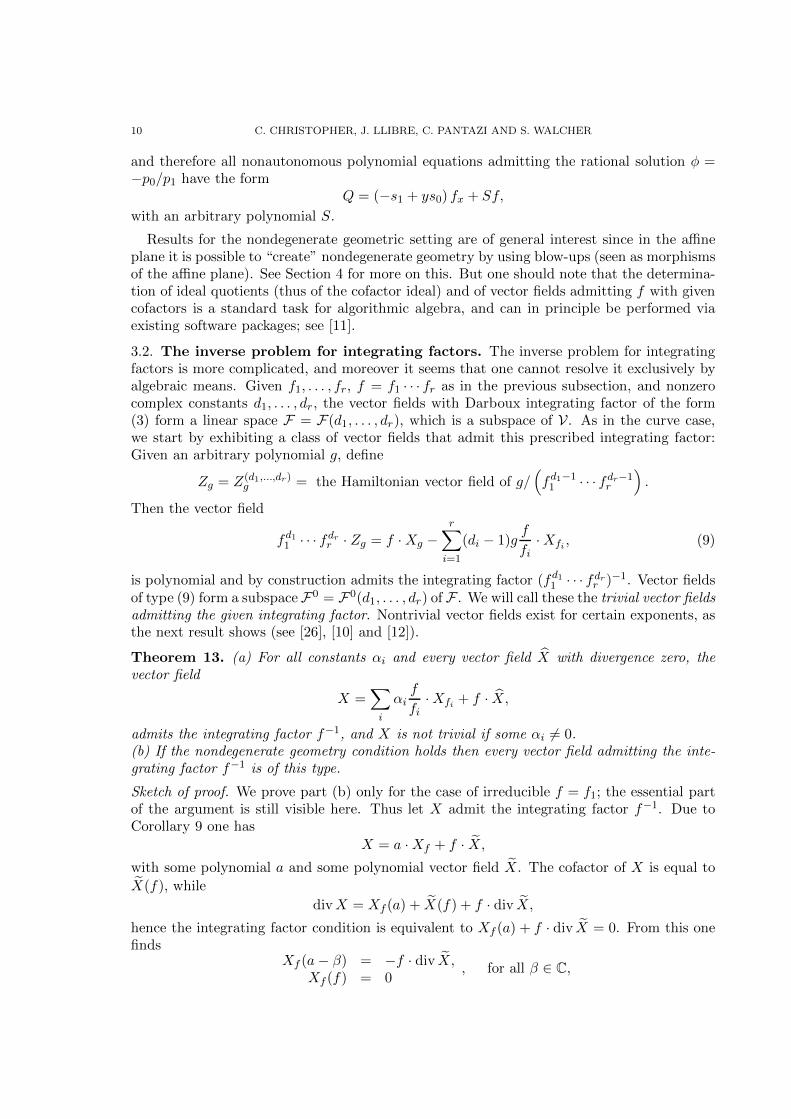
Results for the nondegenerate geometric setting are of general interest since in the affineplane it is possible to “create” nondegenerate geometry by using blow-ups (seen as morphismsof the affine plane). See Section 4 for more on this. But one should note that the determina-tion of ideal quotients (thus of the cofactor ideal) and of vector fields admitting f with givencofactors is a standard task for algorithmic algebra, and can in principle be performed viaexisting software packages; see [11].
3.2. The inverse problem for integrating factors. The inverse problem for integratingfactors is more complicated, and moreover it seems that one cannot resolve it exclusively byalgebraic means. Given f1, . . . , fr, f = f1 · · · fr as in the previous subsection, and nonzerocomplex constants d1, . . . , dr, the vector fields with Darboux integrating factor of the form(3) form a linear space F = F(d1, . . . , dr), which is a subspace of V. As in the curve case,we start by exhibiting a class of vector fields that admit this prescribed integrating factor:Given an arbitrary polynomial g, define
Zg = Z(d1,...,dr)g = the Hamiltonian vector field of g/
(fd1−11 · · · fdr−1
r
).
Then the vector field
fd11 · · · fdr
r · Zg = f ·Xg −r∑
i=1
(di − 1)gf
fi·Xfi , (9)
is polynomial and by construction admits the integrating factor (fd11 · · · fdr
r )−1. Vector fieldsof type (9) form a subspaceF0 = F0(d1, . . . , dr) of F . We will call these the trivial vector fieldsadmitting the given integrating factor. Nontrivial vector fields exist for certain exponents, asthe next result shows (see [26], [10] and [12]).
Theorem 13. (a) For all constants αi and every vector field X with divergence zero, thevector field
X =∑
i
αif
fi·Xfi + f · X,
admits the integrating factor f−1, and X is not trivial if some αi 6= 0.(b) If the nondegenerate geometry condition holds then every vector field admitting the inte-grating factor f−1 is of this type.
Sketch of proof. We prove part (b) only for the case of irreducible f = f1; the essential partof the argument is still visible here. Thus let X admit the integrating factor f−1. Due toCorollary 9 one has
X = a ·Xf + f · X,
with some polynomial a and some polynomial vector field X. The cofactor of X is equal to
X(f), while
divX = Xf (a) + X(f) + f · div X,
hence the integrating factor condition is equivalent to Xf (a) + f · div X = 0. From this onefinds
Xf (a− β) = −f · div X,Xf (f) = 0
, for all β ∈ C,
INVERSE PROBLEMS IN DARBOUX’ THEORY OF INTEGRABILITY 11
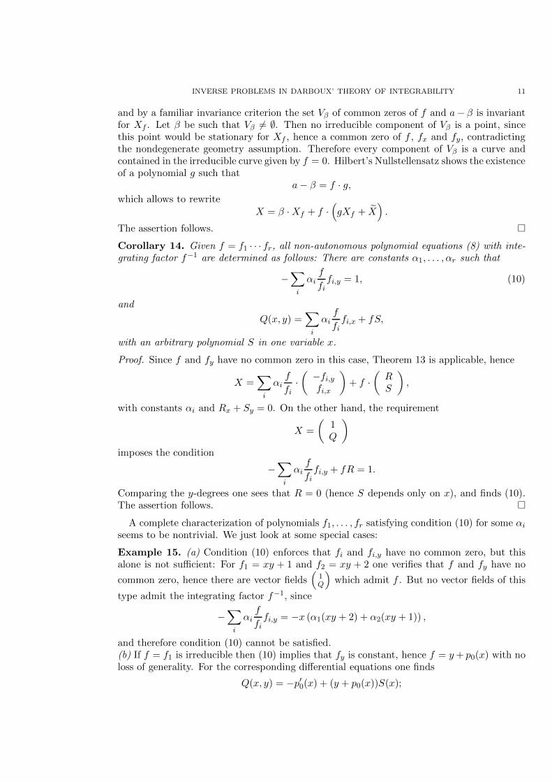
and by a familiar invariance criterion the set Vβ of common zeros of f and a− β is invariantfor Xf . Let β be such that Vβ 6= ∅. Then no irreducible component of Vβ is a point, sincethis point would be stationary for Xf , hence a common zero of f , fx and fy, contradictingthe nondegenerate geometry assumption. Therefore every component of Vβ is a curve andcontained in the irreducible curve given by f = 0. Hilbert’s Nullstellensatz shows the existenceof a polynomial g such that
a− β = f · g,which allows to rewrite
X = β ·Xf + f ·(gXf + X
).
The assertion follows. �Corollary 14. Given f = f1 · · · fr, all non-autonomous polynomial equations (8) with inte-grating factor f−1 are determined as follows: There are constants α1, . . . , αr such that
−∑
i
αif
fifi,y = 1, (10)
and
Q(x, y) =∑
i
αif
fifi,x + fS,
with an arbitrary polynomial S in one variable x.
Proof. Since f and fy have no common zero in this case, Theorem 13 is applicable, hence
X =∑
i
αif
fi·(
−fi,yfi,x
)+ f ·
(RS
),
with constants αi and Rx + Sy = 0. On the other hand, the requirement
X =
(1Q
)
imposes the condition
−∑
i
αif
fifi,y + fR = 1.
Comparing the y-degrees one sees that R = 0 (hence S depends only on x), and finds (10).The assertion follows. �
A complete characterization of polynomials f1, . . . , fr satisfying condition (10) for some αi
seems to be nontrivial. We just look at some special cases:
Example 15. (a) Condition (10) enforces that fi and fi,y have no common zero, but thisalone is not sufficient: For f1 = xy + 1 and f2 = xy + 2 one verifies that f and fy have no
common zero, hence there are vector fields(
1Q
)which admit f . But no vector fields of this
type admit the integrating factor f−1, since
−∑
i
αif
fifi,y = −x (α1(xy + 2) + α2(xy + 1)) ,
and therefore condition (10) cannot be satisfied.(b) If f = f1 is irreducible then (10) implies that fy is constant, hence f = y+ p0(x) with noloss of generality. For the corresponding differential equations one finds
Q(x, y) = −p′0(x) + (y + p0(x))S(x);

12 C. CHRISTOPHER, J. LLIBRE, C. PANTAZI AND S. WALCHER
all of these are linear.(c) If r = 2 and δy(f) = 2 then one has f1 = p1y + p0 and f2 = q1y + q0 with polynomials piand qi in one variable x. One verifies that condition (10) holds if and only if
p0q1 − p1q0 = γ = const.
Without loss of generality we may take γ = 1. For given relatively prime pi, all qi whichsatisfy this relation can be found via Euclid’s algorithm. The corresponding nonautonomousdifferential equations are special Riccati equations.
The following two auxiliary results are elementary but useful, both for examples and fortheoretical purposes.
Lemma 16. Let e1, . . . , er ∈ C and k1, . . . , kr be nonnegative integers. Then
fk11 · · · fkr
r · F0(e1, . . . , er) ⊆ F0(e1 + k1, . . . , er + kr).
Lemma 17. Let
X =
r∑
i=1
aif
fi·Xfi + f · X ∈ V1,
admit the given integrating factor (4), with dℓ 6= 1. Then
X +1
dℓ − 1· fd1
1 · · · fdrr · Zaℓ = fℓ ·X∗,
and X∗ ∈ F(d1, . . . , dℓ − 1, . . . , dr).
From now on and until further notice, nondegenerate geometry will be assumed. ThenLemma 17 yields a reduction strategy, with the starting point that any vector field X admit-ting f is congruent to some fℓ ·X∗ modulo F0(d1, . . . , dr), unless dℓ = 1. In one scenario thisstrategy works perfectly: If all di are positive integers then one can reduce them all to 1 andapply Theorem 13.
Theorem 18. Let the nondegenerate geometry condition be satisfied. If all di are positiveintegers then the elements of F are precisely those of the form
X =∑
i
αifd11 · · · fdr
r
fi·Xfi + fd1
1 · · · fdrr · X,
with constants αi and div X = 0.
In the general case, one might initially hope to apply Lemma 17 repeatedly and reducethe degree of the vector field in every step. But this works only if additional nondegeneracyconditions hold for the stationary points at infinity, see [13] and [10], and will fail in gen-eral. However, one can instead consider the degree δy with respect to y, and start from theassumption
fj = γjynj + terms of smaller degree in y,
with constants γj 6= 0, for all j. This can always be achieved by a suitable invertible lineartransformation and thus involves no loss of generality. A consequence is that in the repre-sentation of X in Lemma 17 one may assume δy(ai) < δy(fi) for all i, since every power yk
with k ≥ δy(fi) can be replaced by a sum of powers of smaller degree, modulo fi. Up to somepoint, one can use this to reduce y-degrees via Lemma 17. A precise statement can be foundin [12], Proposition 8, but for our purposes the following version will suffice.
INVERSE PROBLEMS IN DARBOUX’ THEORY OF INTEGRABILITY 13
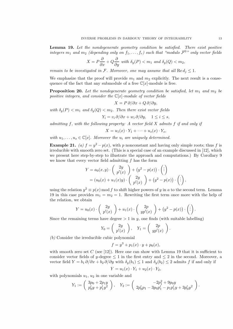
Lemma 19. Let the nondegenerate geometry condition be satisfied. There exist positiveintegers m1 and m2 (depending only on f1, . . . , fr) such that “modulo F0” only vector fields
X = P∂
∂x+Q
∂
∂ywith δy(P ) < m1 and δy(Q) < m2,
remain to be investigated in F . Moreover, one may assume that all Re dj ≤ 1.
We emphasize that the proof will provide m1 and m2 explicitly. The next result is a conse-quence of the fact that any submodule of a free C[x]-module is free.
Proposition 20. Let the nondegenerate geometry condition be satisfied, let m1 and m2 bepositive integers, and consider the C[x]-module of vector fields
X = P ∂/∂x+Q∂/∂y,
with δy(P ) < m1 and δy(Q) < m2. Then there exist vector fields
Yi = vi ∂/∂x+ wi ∂/∂y, 1 ≤ i ≤ s,
admitting f , with the following property: A vector field X admits f if and only if
X = u1(x) · Y1 + · · ·+ us(x) · Ys,
with u1, . . . , us ∈ C[x]. Moreover the ui are uniquely determined.
Example 21. (a) f = y2 − p(x), with p nonconstant and having only simple roots; thus f isirreducible with smooth zero set. (This is a special case of an example discussed in [12], whichwe present here step-by-step to illustrate the approach and computations.) By Corollary 9we know that every vector field admitting f has the form
Y = a0(x, y) ·(
2yp′(x)
)+(y2 − p(x)
)·(...
)
= (u0(x) + u1(x)y) ·(
2yp′(x)
)+(y2 − p(x)
)·(...
),
using the relation y2 ≡ p(x)mod f to shift higher powers of y in a to the second term. Lemma19 in this case provides m1 = m2 = 1. Rewriting the first term once more with the help ofthe relation, we obtain
Y = u0(x) ·(
2yp′(x)
)+ u1(x) ·
(2p
yp′(x)
)+(y2 − p(x)
)·(...
).
Since the remaining terms have degree > 1 in y, one finds (with suitable labelling)
Y0 =
(2y
p′(x)
), Y1 =
(2p
yp′(x)
).
(b) Consider the irreducible cubic polynomial
f = y3 + p1(x) · y + p0(x),
with smooth zero set C (see [12]). Here one can show with Lemma 19 that it is sufficient toconsider vector fields of y-degree ≤ 1 in the first entry and ≤ 2 in the second. Moreover, avector field Y = b1 ∂/∂x + b2 ∂/∂y with δy(b1) ≤ 1 and δy(b2) ≤ 2 admits f if and only if
Y = u1(x) · Y1 + u2(x) · Y2,
with polynomials u1, u2 in one variable and
Y1 :=
(3p0 + 2p1yp′0y + p′1y
2
), Y2 :=
(−2p21 + 9p0y
2p′0p1 − 3p0p′1 − p1p
′1y + 3p′0y
2
).
14 C. CHRISTOPHER, J. LLIBRE, C. PANTAZI AND S. WALCHER
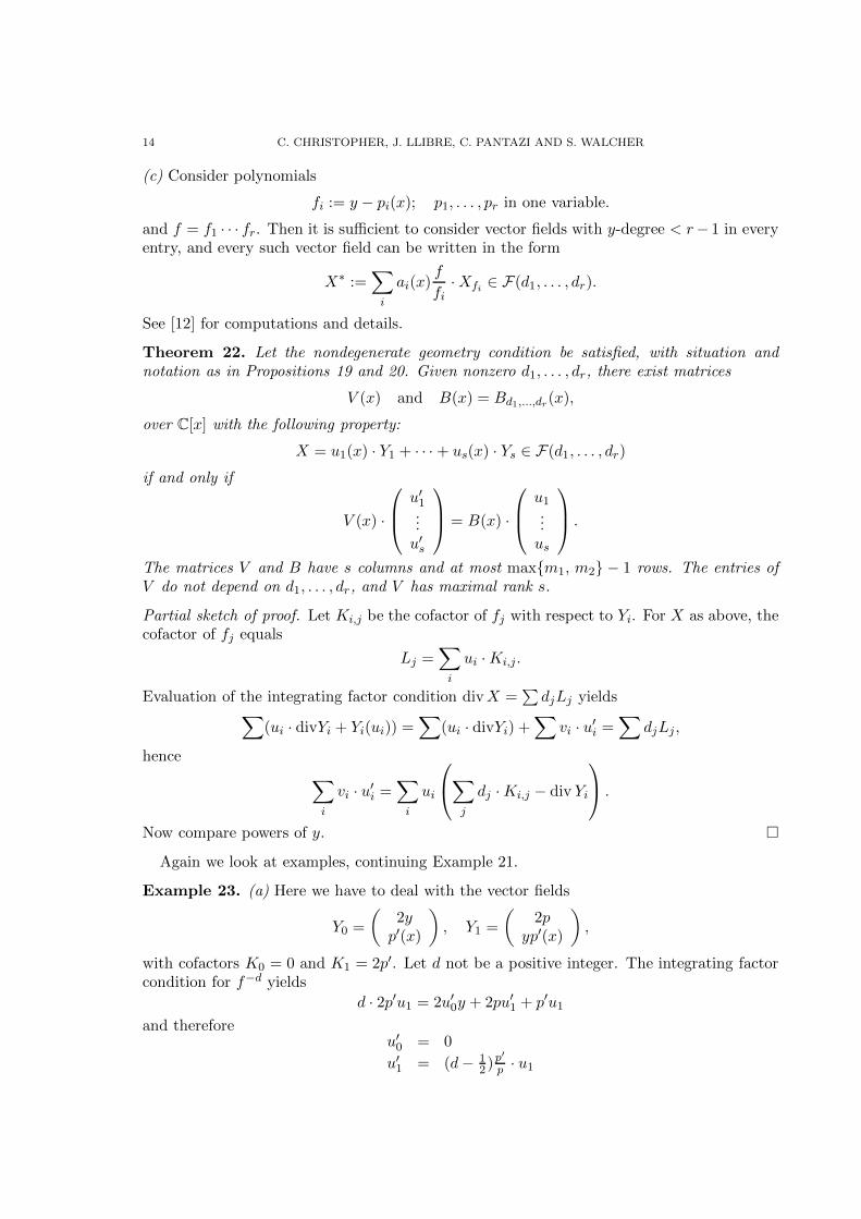
(c) Consider polynomials
fi := y − pi(x); p1, . . . , pr in one variable.
and f = f1 · · · fr. Then it is sufficient to consider vector fields with y-degree < r− 1 in everyentry, and every such vector field can be written in the form
X∗ :=∑
i
ai(x)f
fi·Xfi ∈ F(d1, . . . , dr).
See [12] for computations and details.
Theorem 22. Let the nondegenerate geometry condition be satisfied, with situation andnotation as in Propositions 19 and 20. Given nonzero d1, . . . , dr, there exist matrices
V (x) and B(x) = Bd1,...,dr(x),
over C[x] with the following property:
X = u1(x) · Y1 + · · · + us(x) · Ys ∈ F(d1, . . . , dr)
if and only if
V (x) ·
u′1...u′s
= B(x) ·
u1...us
.
The matrices V and B have s columns and at most max{m1, m2} − 1 rows. The entries ofV do not depend on d1, . . . , dr, and V has maximal rank s.
Partial sketch of proof. Let Ki,j be the cofactor of fj with respect to Yi. For X as above, thecofactor of fj equals
Lj =∑
i
ui ·Ki,j.
Evaluation of the integrating factor condition divX =∑
djLj yields∑
(ui · divYi + Yi(ui)) =∑
(ui · divYi) +∑
vi · u′i =∑
djLj,
hence
∑
i
vi · u′i =∑
i
ui
∑
j
dj ·Ki,j − div Yi
.
Now compare powers of y. �
Again we look at examples, continuing Example 21.
Example 23. (a) Here we have to deal with the vector fields
Y0 =
(2y
p′(x)
), Y1 =
(2p
yp′(x)
),
with cofactors K0 = 0 and K1 = 2p′. Let d not be a positive integer. The integrating factorcondition for f−d yields
d · 2p′u1 = 2u′0y + 2pu′1 + p′u1and therefore
u′0 = 0
u′1 = (d− 12 )
p′p · u1
INVERSE PROBLEMS IN DARBOUX’ THEORY OF INTEGRABILITY 15
This immediately implies that u0 is constant. We will show that u1 = 0 by an approachwhich is unnecessarily complicated for this special problem, but open to generalization: ByLemma 17 one may assume Re d < 0. Write the equation as
u′1 = A(x) · u1with a rational function A. Suppose that u1 =
∑mi=0 bix
i, bm 6= 0. For v = x−1 one then has
du1dv
= −v−2A(v−1) · u1,
which in the present case yields
u1 = bmv−m + · · · , du1dv
= −mbmv−m−1 + · · ·
and
A(v) = (d− 1
2) · nv−1 + · · ·
where the dots indicate terms of higher order in v, and n denotes he degree of p. Comparingcoefficients of v−m−1 shows
−mbm = −(d− 1
2) · nbm,
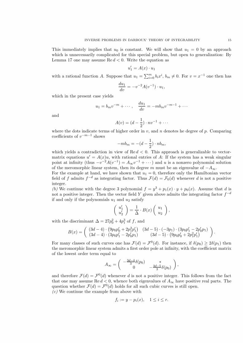
which yields a contradiction in view of Re d < 0. This approach is generalizable to vector-matrix equations u′ = A(x)u, with rational entries of A: If the system has a weak singularpoint at infinity (thus −v−2A(v−1) = A∞v−1 + · · · ) and u is a nonzero polynomial solutionof the meromorphic linear system, then its degree m must be an eigenvalue of −A∞.For the example at hand, we have shown that u1 = 0, therefore only the Hamiltonian vectorfield of f admits f−d as integrating factor. Thus F(d) = F0(d) whenever d is not a positiveinteger.(b) We continue with the degree 3 polynomial f = y3 + p1(x) · y + p0(x). Assume that d isnot a positive integer. Then the vector field Y given above admits the integrating factor f−d
if and only if the polynomials u1 and u2 satisfy(
u′1u′2
)=
1
∆· B(x)
(u1u2
),
with the discriminant ∆ = 27p20 + 4p31 of f , and
B(x) =
((3d− 4) ·
(9p0p
′0 + 2p21p
′1
)(3d− 5) · (−3p1) · (3p0p′1 − 2p′0p1)
(3d − 4) · (3p0p′1 − 2p′0p1) (3d − 5) ·(9p0p
′0 + 2p21p
′1
)).
For many classes of such curves one has F(d) = F0(d). For instance, if δ(p0) ≥ 2δ(p1) thenthe meromorphic linear system admits a first order pole at infinity, with the coefficient matrixof the lowest order term equal to
A∞ =
(−3d−4
3 δ(p0) ∗0 −3d−5
3 δ(p0)
),
and therefore F(d) = F0(d) whenever d is not a positive integer. This follows from the factthat one may assume Re d < 0, whence both eigenvalues of A∞ have positive real parts. Thequestion whether F(d) = F0(d) holds for all such cubic curves is still open.(c) We continue the example from above with
fi := y − pi(x), 1 ≤ i ≤ r.
16 C. CHRISTOPHER, J. LLIBRE, C. PANTAZI AND S. WALCHER
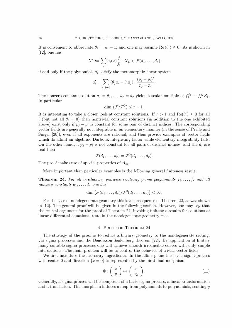
It is convenient to abbreviate θi := di − 1; and one may assume Re (θi) ≤ 0. As is shown in[12], one has
X∗ :=∑
i
ai(x)f
fi·Xfi ∈ F(d1, . . . , dr)
if and only if the polynomials ai satisfy the meromorphic linear system
a′i =∑
j:j 6=i
(θjai − θiaj) ·(pj − pi)
′
pj − pi.
The nonzero constant solution a1 = θ1, . . . , ar = θr yields a scalar multiple of fd11 · · · fdr
r Z1.In particular
dim(F/F0
)≤ r − 1.
It is interesting to take a closer look at constant solutions. If r > 1 and Re(θi) ≤ 0 for alli (but not all θi = 0) then nontrivial constant solutions (in addition to the one exhibitedabove) exist only if pj − pi is constant for some pair of distinct indices. The correspondingvector fields are generally not integrable in an elementary manner (in the sense of Prelle andSinger [20]), even if all exponents are rational, and thus provide examples of vector fieldswhich do admit an algebraic Darboux integrating factor while elementary integrability fails.On the other hand, if pj − pi is not constant for all pairs of distinct indices, and the di arereal then
F(d1, . . . , dr) = F0(d1, . . . , dr).
The proof makes use of special properties of A∞.
More important than particular examples is the following general finiteness result:
Theorem 24. For all irreducible, pairwise relatively prime polynomials f1, . . . , fr and allnonzero constants d1, . . . , dr one has
dim(F(d1, . . . , dr)/F0(d1, . . . , dr)
)< ∞.
For the case of nondegenerate geometry this is a consequence of Theorem 22, as was shownin [12]. The general proof will be given in the following section. However, one may say thatthe crucial argument for the proof of Theorem 24, invoking finiteness results for solutions oflinear differential equations, rests in the nondegenerate geometry case.
4. Proof of Theorem 24
The strategy of the proof is to reduce arbitrary geometry to the nondegenerate setting,via sigma processes and the Bendixson-Seidenberg theorem [22]: By application of finitelymany suitable sigma processes one will achieve smooth irreducible curves with only simpleintersections. The main problem will be to control the behavior of trivial vector fields.
We first introduce the necessary ingredients. In the affine plane the basic sigma processwith center 0 and direction {x = 0} is represented by the birational morphism
Φ :
(xy
)7→(
xxy
). (11)
Generally, a sigma process will be composed of a basic sigma process, a linear transformationand a translation. This morphism induces a map from polynomials to polynomials, sending g
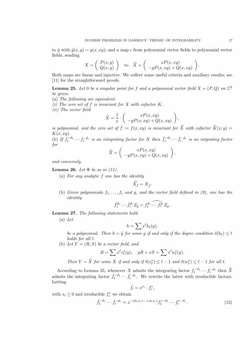
INVERSE PROBLEMS IN DARBOUX’ THEORY OF INTEGRABILITY 17
to g with g(x, y) = g(x, xy); and a map ι from polynomial vector fields to polynomial vectorfields, sending
X =
(P (x, y)Q(x, y)
)to X =
(xP (x, xy)
−yP (x, xy) +Q(x, xy)
).
Both maps are linear and injective. We collect some useful criteria and auxiliary results; see[11] for the straightforward proofs.
Lemma 25. Let 0 be a singular point for f and a polynomial vector field X = (P,Q) on C2
be given.(a) The following are equivalent:(i) The zero set of f is invariant for X with cofactor K.(ii) The vector field
X =1
x·(
xP (x, xy)−yP (x, xy) +Q(x, xy)
),
is polynomial, and the zero set of f := f(x, xy) is invariant for X with cofactor K(x, y) =K(x, xy).
(b) If f−d11 · · · f−dr
r is an integrating factor for X then f−d11 · · · f−dr
r is an intgrating factorfor
X =
(xP (x, xy)
−yP (x, xy) +Q(x, xy)
),
and conversely.
Lemma 26. Let Φ be as in (11).
(a) For any analytic f one has the identity
Xf = X bf.
(b) Given polynomials f1, . . . , fr and g, and the vector field defined in (9), one has theidentity
fd11 · · · fdr
r Zbg =fd1
1 · · · fdrr Zg.
Lemma 27. The following statements hold.
(a) Let
h =∑
xℓhℓ(y),
be a polynomial. Then h = g for some g if and only if the degree condition δ(hℓ) ≤ ℓholds for all ℓ.
(b) Let Y = (R,S) be a vector field, and
R =∑
xℓv∗ℓ (y), yR+ xS =∑
xℓw∗ℓ (y).
Then Y = X for some X if and only if δ(v∗ℓ ) ≤ ℓ− 1 and δ(w∗ℓ ) ≤ ℓ− 1 for all ℓ.
According to Lemma 25, whenever X admits the integrating factor f−d11 · · · f−dr
r then X
admits the integrating factor f−d11 · · · f−dr
r . We rewrite the latter with irreducible factors.Letting
fi = xsi · f∗i ,
with si ≥ 0 and irreducible f∗i we obtain
f−d11 · · · f−dr
r = x−(d1s1+...+drsr)f∗1−d1 · · · f∗
r−dr . (12)
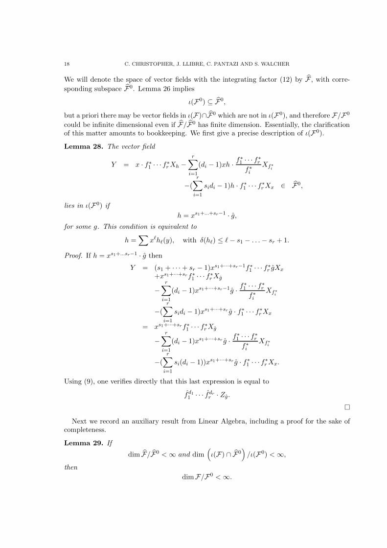
18 C. CHRISTOPHER, J. LLIBRE, C. PANTAZI AND S. WALCHER
We will denote the space of vector fields with the integrating factor (12) by F , with corre-
sponding subspace F0. Lemma 26 implies
ι(F0) ⊆ F0,
but a priori there may be vector fields in ι(F)∩F0 which are not in ι(F0), and therefore F/F0
could be infinite dimensional even if F/F0 has finite dimension. Essentially, the clarificationof this matter amounts to bookkeeping. We first give a precise description of ι(F0).
Lemma 28. The vector field
Y = x · f∗1 · · · f∗
rXh −r∑
i=1
(di − 1)xh · f∗1 · · · f∗
r
f∗i
Xf∗i
−(
r∑
i=1
sidi − 1)h · f∗1 · · · f∗
rXx ∈ F0,
lies in ι(F0) if
h = xs1+...+sr−1 · g,for some g. This condition is equivalent to
h =∑
xℓhℓ(y), with δ(hℓ) ≤ ℓ− s1 − . . .− sr + 1.
Proof. If h = xs1+...sr−1 · g then
Y = (s1 + · · ·+ sr − 1)xs1+···+sr−1f∗1 · · · f∗
r gXx
+xs1+···+srf∗1 · · · f∗
rXg
−r∑
i=1
(di − 1)xs1+···+sr−1g · f∗1 · · · f∗
r
f∗i
Xf∗i
−(
r∑
i=1
sidi − 1)xs1+···+sr g · f∗1 · · · f∗
rXx
= xs1+···+srf∗1 · · · f∗
rXg
−r∑
i=1
(di − 1)xs1+···+sr g · f∗1 · · · f∗
r
f∗i
Xf∗i
−(
r∑
i=1
si(di − 1))xs1+···+sr g · f∗1 · · · f∗
rXx.
Using (9), one verifies directly that this last expression is equal to
fd11 · · · fdr
r · Zg.
�
Next we record an auxiliary result from Linear Algebra, including a proof for the sake ofcompleteness.
Lemma 29. If
dim F/F0 < ∞ and dim(ι(F) ∩ F0
)/ι(F0) < ∞,
then
dimF/F0 < ∞.
INVERSE PROBLEMS IN DARBOUX’ THEORY OF INTEGRABILITY 19
Proof. We assume that
dim F/F0 < ∞ and dimF/F0 = ∞,
and let Xi ∈ F , i = 1, 2, . . . be an infinite system such that (Xi + F0)i≥1 is linearly in-
dependent. Since dim F/F0 < ∞, we may assume after possible relabeling that there
is some q ≥ 1 such that(X1 + F0, . . . , Xq−1 + F0
)is a linearly independent system but
X1+ F0, . . . , Xq−1+ F0, Xq−1+i+ F0 are linearly dependent for every i ≥ 1. Therefore thereexist scalars βij such that
Xq−1+i −q−1∑
j=1
βijXj ∈ F0, all i ≥ 1.
We define
Yi := Xq−1+i −q−1∑
j=1
βijXj ∈ F , i ≥ 1.
Then (Yi + F0) is an infinite linearly independent system. Since ι is injective, the system
(Yi + ι(F0)) is also linearly independent. Therefore
dim(ι(F) ∩ F0
)/ι(F0) = ∞.
�
Now we write
f∗i =
∑xℓfi,ℓ(y), (13)
and note that δ(fi,ℓ) ≤ si + ℓ by construction. Moreover we may assume that δ(fi,0) = si:This can be achieved via a linear automorphism x 7→ x+αy, y 7→ y with suitable α. In otherwords, this can be achieved by suitable choice of direction of the sigma process, and onlyfinitely many directions have to be excluded. Moreover, we are only interested in the case ofa degenerate singular point at 0, thus
∑si ≥ 2.
Lemma 30. If δ(f0,i) = si for i = 1, . . . , r, and∑
si ≥ 2, then
ι(F) ∩ F0 = ι(F0).
Proof. (i) We consider the vector field Y ∈ F0 as in Lemma 28, and we abbreviate Y = (R,S).Then
R = x
(−f∗
1 · · · f∗r hy + (
r∑
i=1
(di − 1)f∗1 · · · f∗
r
f∗i
f∗i y)h
)= x ·
∑xℓvℓ(y). (14)
According to Lemma 27 we have Y ∈ ι(F) only if δ(vℓ) ≤ ℓ for all ℓ. Moreover we have
yR+ xS = yR
+ x
(f∗1 · · · f∗
r xhx −∑
(di − 1)hf∗1 · · · f∗
r
f∗i
xfix
)
−x((∑
sidi − 1)hf∗1 · · · f∗
r
).
According to Lemma 27 we have Y ∈ ι(F) only if yR+ xS is of the form
x ·∑
xℓwℓ(y), δ(wℓ) ≤ ℓ.
20 C. CHRISTOPHER, J. LLIBRE, C. PANTAZI AND S. WALCHER
Combining this with the condition on R, we find that Y ∈ ι(F) only if
f∗1 · · · f∗
r xhx −∑
(di − 1)hf∗1 · · · f∗
r
f∗i
xfix
−(∑
sidi − 1)hf∗1 · · · f∗
r =∑
xℓwℓ,(15)
with δ(wℓ) ≤ ℓ+ 1 for all ℓ. We will evaluate (14) and (15) degree by degree in x. Thus wewrite
h =∑
xℓhℓ(y),
and note thathy =
∑xℓh′ℓ(y), xhx =
∑ℓxℓhℓ(y).
From (13) we have
f∗i y =
∑xℓf ′
i,ℓ(y), xf∗i x =
∑ℓxℓfi,ℓ(y).
The degree by degree evaluation of (14) yields
vℓ = −f1,0 · · · fr,0 · h′ℓ + (
r∑
i=1
(di − 1)f1,0 · · · fr,0
fi,0fi,0
′) · hℓ
−∑
j1,...,jr
f1,j1 · · · fr,jrh′ℓ−(j1+···jr)
+∑
j1,...,jr
∑
i
(di − 1)f1,j1 · · · fr,jr
fi,jif ′i,jihℓ−(j1+···jr),
(16)
where the summation extends over all tuples (j1, . . . , jr) of nonnegative integers such that1 ≤∑ ji ≤ ℓ. The degree by degree evaluation of (15) yields
wℓ = (ℓ−∑i sidi + 1)f1,0 · · · fr,0 · hℓ+
∑
j1,...,jr
(ℓ−∑
i
diji −∑
i
disi + 1)f1,j1 · · · fr,jrhℓ−(j1+···jr), (17)
with the same range for (j1, . . . , jr).
(ii) Given a nonzero polynomial p, the polynomial
−f1,0 · · · fr,0 · p′ + (
r∑
i=1
(di − 1)f1,0 · · · fr,0
fi,0fi,0
′) · p,
has degree < δ(p) + s1 + · · ·+ sr − 1 only if
δ(p) =∑
si(di − 1).
To see this we note that the coefficient of the term of degree δ(p) + s1 + · · ·+ sr − 1 is equalto the product of the leading coefficients of the fi,0 and p, and the factor
−δ(p) +∑
si(di − 1).
(iii) We will prove by induction on ℓ: If the vector field Y from Lemma 28 lies in ι(F) then
δ(hℓ) ≤ ℓ−∑
si + 1,
with the tacit understanding that δ(hℓ) < 0 means hℓ = 0. We will use the degree conditionsin (16) and (17).
ℓ = 0: In the case that∑
sidi − 1 6= 0, the assumption h0 6= 0 and (17) lead to
s1 + · · ·+ sr + δ(h0) = δ(f1,0 · · · fr,0 · h0) ≤ 1;
INVERSE PROBLEMS IN DARBOUX’ THEORY OF INTEGRABILITY 21
a contradiction. In the case∑
sidi − 1 = 0, the assumption h0 6= 0, part (ii) and the degreecondition in (16) lead to
δ(h0) =∑
sidi −∑
si = 1−∑
si < 0;
which also gives a contradiction.
For the induction step we assume that the assertion holds for all hℓ−j , with 1 ≤ j ≤ ℓ.Since the degree of fi,ji is at most equal to si + ji, every term on the right-hand side of (16),with the possible exception of those involving hℓ, has degree ≤ ℓ. By the same argument,every term on the right-hand side of (17), with the possible exception of those involving hℓ,has degree ≤ ℓ+ 1. Therefore we have
δ
(−f1,0 · · · fr,0 · h′ℓ + (
r∑
i=1
(di − 1)f1,0 · · · fr,0
fi,0fi,0
′) · hℓ)
≤ ℓ,
as well as
δ
((ℓ−
∑
i
sidi + 1)f1,0 · · · fr,0 · hℓ)
≤ ℓ+ 1,
by the induction hypothesis. In the case that ℓ 6= ∑ sidi − 1, the second condition directlyshows δ(hℓ) ≤ ℓ−∑ si + 1, as desired. In the case ℓ =
∑sidi − 1, the assumption δ(hℓ) >
ℓ−∑ si + 1 implies that highest-degree terms in (16) must cancel. By part (ii) this implies
δ(hℓ) =∑
sidi −∑
si = ℓ−∑
si + 1,
an obvious contradiction. �This leads us to the proof of our main result.
Proof of Theorem 24. The Bendixson-Seidenberg theorem for Xf , cf. Seidenberg [22], andLemma 26 show that a finite number of sigma processes, with suitable centers and directions,will transform the fi to polynomials fi which satisfy the geometric nondegeneracy condition.In every single sigma process at most finitely many directions have to be excluded, as can beseen from [22]. For f1, . . . , fr and d1, . . . , dr finiteness holds by Theorem 11 and Theorem 3of [12].For a single sigma process at a degenerate singular point, with a suitably chosen direction,Lemma 29 and Lemma 30 show that finiteness holds for the original setting if it holds for thetransformed polynomials. Induction on the number of sigma processes finishes the proof. �Remark 31. Classically, one knows that sigma processes can be used directly to simplifysingular points of curves; see Shafarevich [23], Ch. II, §4 (including Exercises). We chose thedetour via vector fields because Seidenberg gives a complete proof which shows clearly thatthe exclusion of finitely many directions does not matter.
References
[1] P.B. Acosta-Humanez, J.T. Lazaro, J.J. Morales-Ruiz, C. Pantazi: On the integrability of polynomialfields in the plane by means of Picard-Vessiot theory. Preprint, 27 pp., arXiv:1012.4796v2 (2011).
[2] C. Camacho, P. Sad: Invariant varieties through singularities of holomorphic vector fields. Ann. Math.15 (1982), 579–595.
[3] M. Carnicer: The Poincare problem in the nondicritical case. Ann. Math. 140 (1994), 289–294.[4] D. Cerveau, A. Lins Neto: Holomorphic foliations in CP (2) having an invariant algebraic curve. Ann.
Inst. Fourier 41 (1991), 883–903.[5] J. Chavarriga, J. Llibre: Invariant algebraic curves and rational first integrals for planar polynomial vector
fields. J. Differential Eqs. 169 (2001), 1–16.

22 C. CHRISTOPHER, J. LLIBRE, C. PANTAZI AND S. WALCHER
[6] J. Chavarriga, H. Giacomini, J. Gine, J. Llibre: Darboux integrability and the inverse integrating factor.J. Differential Eqs. 194 (2003), 116–139.
[7] C. Christopher: Liouvillian first integrals of second order polynomial differential equations. Electronic J.Diff. Eqs. 1999, no. 49 (1999), 1–7.
[8] C. Christopher, J. Llibre: Algebraic aspects of integrability for polynomial systems. Qualitative Theory ofDynamical Systems 1 (1999), 71–95.
[9] C. Christopher, J. Llibre: Integrability via invariant algebraic curves for planar polynomial differentialsystems. Annals of Differential Equations 16 (2000), 5–19.
[10] C. Christopher, J. Llibre, C. Pantazi, S. Walcher: Inverse problems for multiple invariant curves. Proc.Roy. Soc. Edinburgh 137A (2007), 1197 – 1226.
[11] C. Christopher, J. Llibre, C. Pantazi, S. Walcher: Inverse problems for invariant algebraic curves: Explicitcomputations. Proc. Roy. Soc. Edinburgh 139A (2009), 1 –16.
[12] C. Christopher, J. Llibre, C. Pantazi, S. Walcher: Darboux integrating factors: Inverse problems. J.Differential Eqs. 250 (2011), 1– 25.
[13] C. Christopher, J. Llibre, C. Pantazi, X. Zhang: Darboux integrability and invariant algebraic curves forplanar polynomial systems. J. Phys. A 35 (2002), 2457–2476.
[14] S.C. Coutinho, L. Menasche Schechter: Algebraic solutions of plane vector fields. J. Pure Appl. Algebra213 (2009), 144–153 .
[15] G. Darboux: Memoire sur les equations differentielles algebriques du premier ordre et du premier degre(Melanges). Bull. Sci. math. 2eme serie 2 (1878), 60–96; 123–144; 151–200.
[16] E.L. Ince: Ordinary differential equations. Dover Publ., New York (1956).[17] J.P. Jouanolou: Equations de Pfaff algebriques. Lectures Notes in Mathematics 708, Springer-Verlag,
New York/Berlin, 1979.[18] J. Llibre, G. Rodriguez: Configurations of limit cycles and planar polynomial vector fields. J. Differential
Eqs. 198 (2004), 374–380.[19] P.J. Olver: Applications of Lie groups to differential equations. Springer-Verlag, Berlin/New York 1986.[20] M. J. Prelle and M. F. Singer: Elementary first integrals of differential equations. Trans. Amer. Math.
Soc. 279 (1983), 613–636.[21] M. van der Put, M. Singer: Galois theory in linear differential equations. Springer-Verlag, New York
(2003).[22] A. Seidenberg: Reduction of singularities of the differential equation Ady = Bdx. Amer. J. Math. 40
(1968), 248 –269.[23] I.R. Shafarevich: Basic algebraic geometry. Springer-Verlag, Berlin 1977.[24] M.F. Singer: Liouvillian first integrals of differential equations. Trans. Amer. Math. Soc. 333 (1992),
673–688.[25] B.L. van der Waerden: Algebra I, II. Springer, New York (1991).[26] S. Walcher: Plane polynomial vector fields with prescribed invariant curves. Proc. Royal Soc. Edinburgh
130A (2000), 633 – 649.[27] S. Walcher: On the Poincare problem. J. Differential Eqs. 166 (2000), 51–78.
1Department of Mathematics and Statistics, University of Plymouth, Plymouth PL2 3AJ,U.K.
E-mail address: [email protected]
2 Departament de Matematiques, Universitat Autonoma de Barcelona, Edifici C, 08193 Bel-laterra, Barcelona, Catalonia, Spain
E-mail address: [email protected]
3 Departament de Matematica Aplicada I, Universitat Politecnica de Catalunya, (EPSEB),Av. Doctor Maranon, 44–50, 08028 Barcelona, Catalonia, Spain
E-mail address: [email protected]
4 Lehrstuhl A fur Mathematik, RWTH Aachen, 52056 Aachen, GermanyE-mail address: [email protected]