Inverse Problems: Exercices - Jussieutarantola/exercices/chapter_05/Radiative.pdf · Individual Sections of the Book Inverse Problems: Exercices With mathematica, matlab, and scilab

Individual Sections of the Book

Inverse Problems: Exercices

With mathematica, matlab, and scilab solutions

Albert Tarantola1

Université de Paris, Institut de Physique du Globe4, place Jussieu; 75005 Paris; France

E-mail: [email protected]

March 12, 2007

1© A. Tarantola, 2006. Students and professors are invited to freely use this text.

5.2 Plant Leafs and the Radiative Model 141

5.2 Plant Leafs and the Radiative Model

Section written with the collaboration of Jean-Pierre Frangi.

Note: explain here the background of this problem, why one is interested in studying theoptical properties of a compact plant leaf, and the industrial interest of these developments.

5.2.1 The radiative transfer model

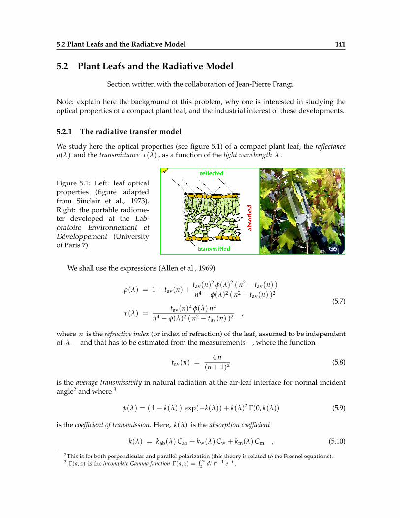
We study here the optical properties (see figure 5.1) of a compact plant leaf, the reflectanceρ(λ) and the transmittance τ(λ) , as a function of the light wavelength λ .

Figure 5.1: Left: leaf opticalproperties (figure adaptedfrom Sinclair et al., 1973).Right: the portable radiome-ter developed at the Lab-oratoire Environnement etDéveloppement (Universityof Paris 7).

We shall use the expressions (Allen et al., 1969)

ρ(λ) = 1− tav(n) +tav(n)2 φ(λ)2 ( n2 − tav(n) )n4 − φ(λ)2 ( n2 − tav(n) )2

τ(λ) =tav(n)2 φ(λ) n2

n4 − φ(λ)2 ( n2 − tav(n) )2 ,

(5.7)

where n is the refractive index (or index of refraction) of the leaf, assumed to be independentof λ —and that has to be estimated from the measurements—, where the function

tav(n) =4 n

(n + 1)2 (5.8)

is the average transmissivity in natural radiation at the air-leaf interface for normal incidentangle2 and where 3

φ(λ) = ( 1− k(λ) ) exp(−k(λ)) + k(λ)2 Γ(0, k(λ)) (5.9)

is the coefficient of transmission. Here, k(λ) is the absorption coefficient

k(λ) = kab(λ) Cab + kw(λ) Cw + km(λ) Cm , (5.10)

2This is for both perpendicular and parallel polarization (this theory is related to the Fresnel equations).3 Γ(a, z) is the incomplete Gamma function Γ(a, z) =

∫ ∞z dt ta−1 e−t .

142 Nonlinear Least Squares

where kab(λ) is the specific absorption coefficient for total chlorophyll, kw(λ) that of water, andkm(λ) that of dry matter. Finally, Cab is the chlorophyll concentration (typically expressed inµg/cm2), Cw is the equivalent water thickness (typically expressed in cm), and Cm is the drymatter content (typically expressed in g/cm2).

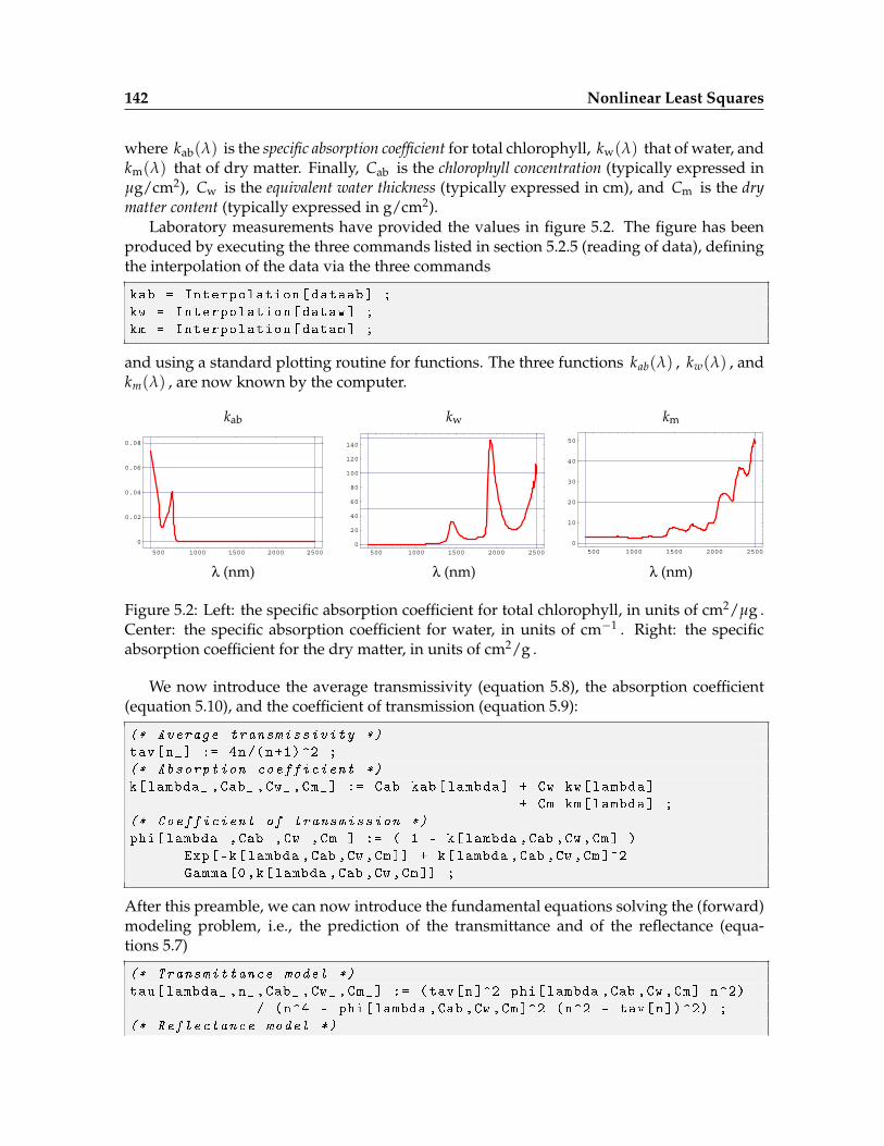
Laboratory measurements have provided the values in figure 5.2. The figure has beenproduced by executing the three commands listed in section 5.2.5 (reading of data), definingthe interpolation of the data via the three commands

kab = Interpolation[dataab] ;

kw = Interpolation[dataw] ;

km = Interpolation[datam] ;

and using a standard plotting routine for functions. The three functions kab(λ) , kw(λ) , andkm(λ) , are now known by the computer.

500 1000 1500 2000 2500

0

0.02

0.04

0.06

0.08

500 1000 1500 2000 25000

20

40

60

80

100

120

140

500 1000 1500 2000 25000

10

20

30

40

50

kab kmkw

! (nm) ! (nm) ! (nm)

Figure 5.2: Left: the specific absorption coefficient for total chlorophyll, in units of cm2/µg .Center: the specific absorption coefficient for water, in units of cm−1 . Right: the specificabsorption coefficient for the dry matter, in units of cm2/g .

We now introduce the average transmissivity (equation 5.8), the absorption coefficient(equation 5.10), and the coefficient of transmission (equation 5.9):

(* Average transmissivity *)

tav[n_] := 4n/(n+1)^2 ;

(* Absorption coefficient *)

k[lambda_ ,Cab_ ,Cw_ ,Cm_] := Cab kab[lambda] + Cw kw[lambda]

+ Cm km[lambda] ;

(* Coefficient of transmission *)

phi[lambda_ ,Cab_ ,Cw_ ,Cm_] := ( 1 - k[lambda ,Cab ,Cw,Cm] )

Exp[-k[lambda ,Cab ,Cw ,Cm]] + k[lambda ,Cab ,Cw ,Cm]^2

Gamma[0,k[lambda ,Cab ,Cw,Cm]] ;

After this preamble, we can now introduce the fundamental equations solving the (forward)modeling problem, i.e., the prediction of the transmittance and of the reflectance (equa-tions 5.7)

(* Transmittance model *)

tau[lambda_ ,n_ ,Cab_ ,Cw_ ,Cm_] := (tav[n]^2 phi[lambda ,Cab ,Cw ,Cm] n^2)

/ (n^4 - phi[lambda ,Cab ,Cw ,Cm]^2 (n^2 - tav[n])^2) ;

(* Reflectance model *)


rho[lambda_ ,n_ ,Cab_ ,Cw_ ,Cm_] := 1 - tav[n] + ( (tav[n]^2

phi[lambda ,Cab ,Cw ,Cm]^2 (n^2 - tav[n]) )

/ ( n^4 - phi[lambda ,Cab ,Cw,Cm]^2 (n^2 - tav[n])^2) ) ;

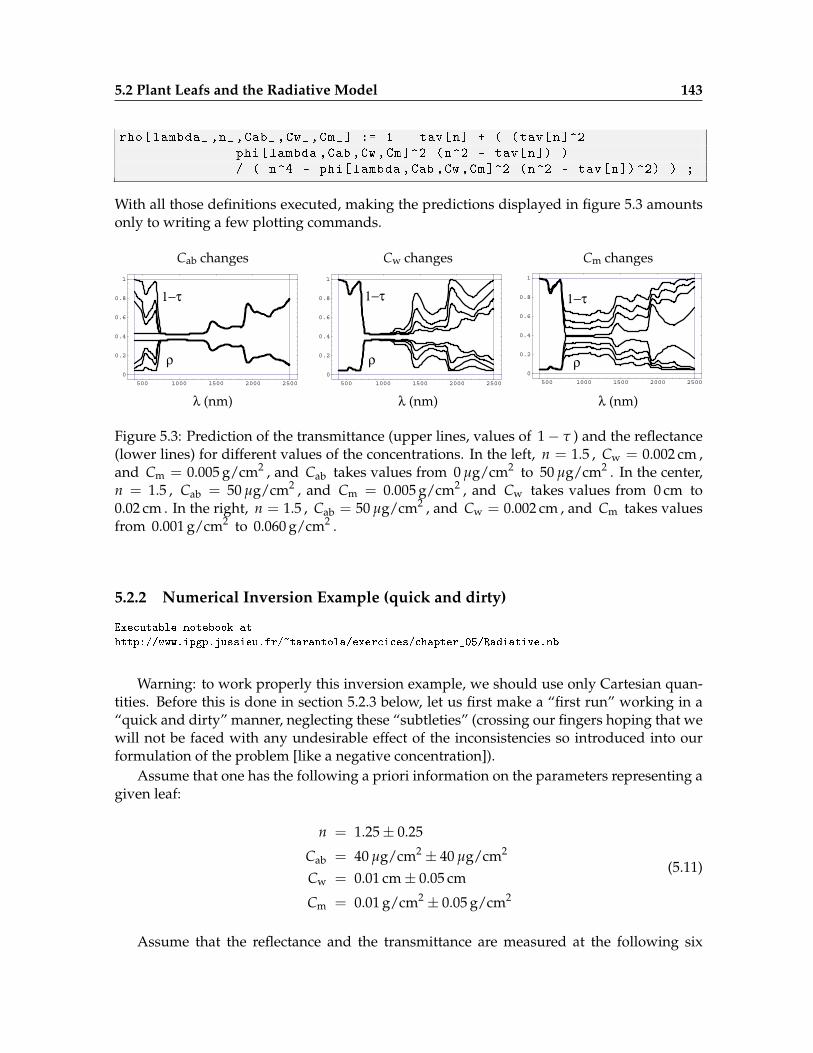
With all those definitions executed, making the predictions displayed in figure 5.3 amountsonly to writing a few plotting commands.

1!" 1!" 1!"

500 1000 1500 2000 25000

0.2

0.4

0.6

0.8

1

500 1000 1500 2000 25000

0.2

0.4

0.6

0.8

1

500 1000 1500 2000 25000

0.2

0.4

0.6

0.8

1

# (nm) # (nm) # (nm)

Cab changes Cw changes Cm changes

$ $ $

Figure 5.3: Prediction of the transmittance (upper lines, values of 1− τ ) and the reflectance(lower lines) for different values of the concentrations. In the left, n = 1.5 , Cw = 0.002 cm ,and Cm = 0.005 g/cm2 , and Cab takes values from 0 µg/cm2 to 50 µg/cm2 . In the center,n = 1.5 , Cab = 50 µg/cm2 , and Cm = 0.005 g/cm2 , and Cw takes values from 0 cm to0.02 cm . In the right, n = 1.5 , Cab = 50 µg/cm2 , and Cw = 0.002 cm , and Cm takes valuesfrom 0.001 g/cm2 to 0.060 g/cm2 .

5.2.2 Numerical Inversion Example (quick and dirty)

Executable notebook at

http://www.ipgp.jussieu.fr/~tarantola/exercices/chapter_05/Radiative.nb

Warning: to work properly this inversion example, we should use only Cartesian quan-tities. Before this is done in section 5.2.3 below, let us first make a “first run” working in a“quick and dirty” manner, neglecting these “subtleties” (crossing our fingers hoping that wewill not be faced with any undesirable effect of the inconsistencies so introduced into ourformulation of the problem [like a negative concentration]).

Assume that one has the following a priori information on the parameters representing agiven leaf:

n = 1.25± 0.25

Cab = 40 µg/cm2 ± 40 µg/cm2

Cw = 0.01 cm± 0.05 cm

Cm = 0.01 g/cm2 ± 0.05 g/cm2

(5.11)

Assume that the reflectance and the transmittance are measured at the following six


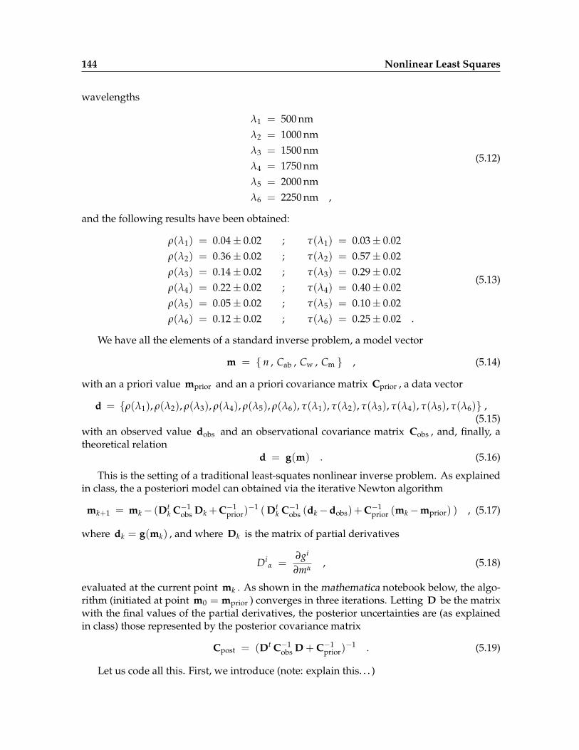
wavelengths

λ1 = 500 nmλ2 = 1000 nmλ3 = 1500 nmλ4 = 1750 nmλ5 = 2000 nmλ6 = 2250 nm ,

(5.12)

and the following results have been obtained:

ρ(λ1) = 0.04± 0.02 ; τ(λ1) = 0.03± 0.02ρ(λ2) = 0.36± 0.02 ; τ(λ2) = 0.57± 0.02ρ(λ3) = 0.14± 0.02 ; τ(λ3) = 0.29± 0.02ρ(λ4) = 0.22± 0.02 ; τ(λ4) = 0.40± 0.02ρ(λ5) = 0.05± 0.02 ; τ(λ5) = 0.10± 0.02ρ(λ6) = 0.12± 0.02 ; τ(λ6) = 0.25± 0.02 .

(5.13)

We have all the elements of a standard inverse problem, a model vector

m = { n , Cab , Cw , Cm } , (5.14)

with an a priori value mprior and an a priori covariance matrix Cprior , a data vector

d = {ρ(λ1), ρ(λ2), ρ(λ3), ρ(λ4), ρ(λ5), ρ(λ6), τ(λ1), τ(λ2), τ(λ3), τ(λ4), τ(λ5), τ(λ6)} ,(5.15)

with an observed value dobs and an observational covariance matrix Cobs , and, finally, atheoretical relation

d = g(m) . (5.16)

This is the setting of a traditional least-squates nonlinear inverse problem. As explainedin class, the a posteriori model can obtained via the iterative Newton algorithm

mk+1 = mk− (Dtk C−1

obs Dk + C−1prior)

−1 ( Dtk C−1

obs (dk−dobs)+ C−1prior (mk−mprior) ) , (5.17)

where dk = g(mk) , and where Dk is the matrix of partial derivatives

Diα =

∂gi

∂mα, (5.18)

evaluated at the current point mk . As shown in the mathematica notebook below, the algo-rithm (initiated at point m0 = mprior ) converges in three iterations. Letting D be the matrixwith the final values of the partial derivatives, the posterior uncertainties are (as explainedin class) those represented by the posterior covariance matrix

Cpost = (Dt C−1obs D + C−1

prior)−1 . (5.19)

Let us code all this. First, we introduce (note: explain this. . . )


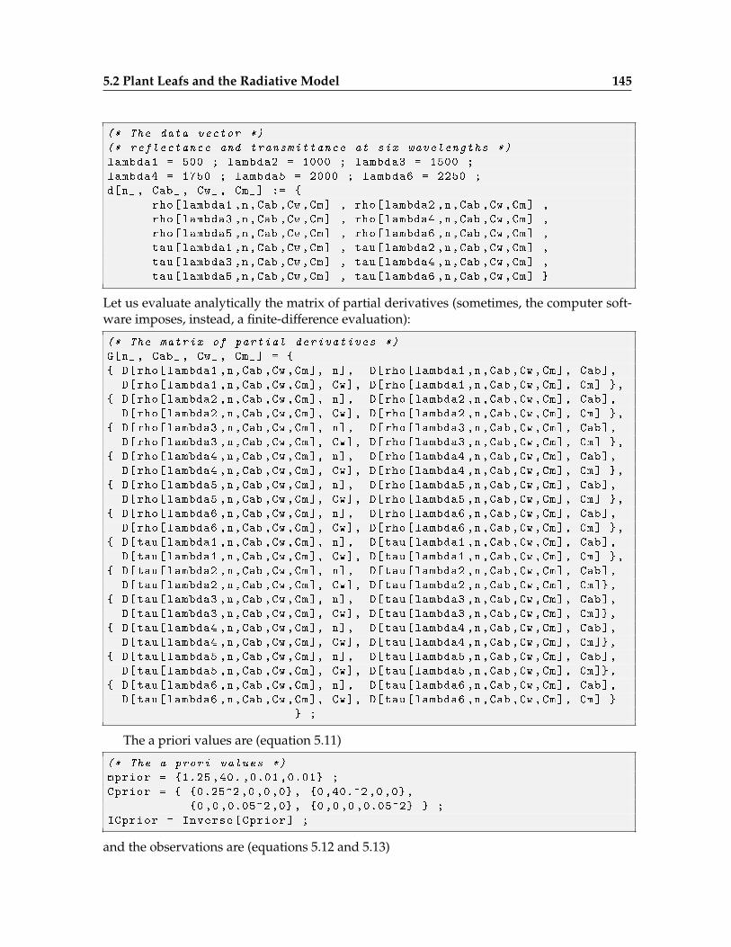
(* The data vector *)

(* reflectance and transmittance at six wavelengths *)

lambda1 = 500 ; lambda2 = 1000 ; lambda3 = 1500 ;

lambda4 = 1750 ; lambda5 = 2000 ; lambda6 = 2250 ;

d[n_, Cab_ , Cw_ , Cm_] := {

rho[lambda1 ,n,Cab ,Cw ,Cm] , rho[lambda2 ,n,Cab ,Cw ,Cm] ,



tau[lambda1 ,n,Cab ,Cw ,Cm] , tau[lambda2 ,n,Cab ,Cw ,Cm] ,

tau[lambda3 ,n,Cab ,Cw ,Cm] , tau[lambda4 ,n,Cab ,Cw ,Cm] ,

tau[lambda5 ,n,Cab ,Cw ,Cm] , tau[lambda6 ,n,Cab ,Cw ,Cm] }

Let us evaluate analytically the matrix of partial derivatives (sometimes, the computer soft-ware imposes, instead, a finite-difference evaluation):

(* The matrix of partial derivatives *)

G[n_, Cab_ , Cw_ , Cm_] = {

{ D[rho[lambda1 ,n,Cab ,Cw ,Cm], n], D[rho[lambda1 ,n,Cab ,Cw ,Cm], Cab],

D[rho[lambda1 ,n,Cab ,Cw,Cm], Cw], D[rho[lambda1 ,n,Cab ,Cw,Cm], Cm] },











{ D[tau[lambda1 ,n,Cab ,Cw ,Cm], n], D[tau[lambda1 ,n,Cab ,Cw ,Cm], Cab],

D[tau[lambda1 ,n,Cab ,Cw,Cm], Cw], D[tau[lambda1 ,n,Cab ,Cw,Cm], Cm] },


D[tau[lambda2 ,n,Cab ,Cw,Cm], Cw], D[tau[lambda2 ,n,Cab ,Cw,Cm], Cm]},








D[tau[lambda6 ,n,Cab ,Cw,Cm], Cw], D[tau[lambda6 ,n,Cab ,Cw,Cm], Cm] }

} ;

The a priori values are (equation 5.11)

(* The a prori values *)

mprior = {1.25 ,40. ,0.01 ,0.01} ;

Cprior = { {0.25^2,0 ,0 ,0} , {0,40.^2,0,0},

{0,0 ,0.05^2 ,0} , {0 ,0 ,0 ,0.05^2} } ;

ICprior = Inverse[Cprior] ;

and the observations are (equations 5.12 and 5.13)


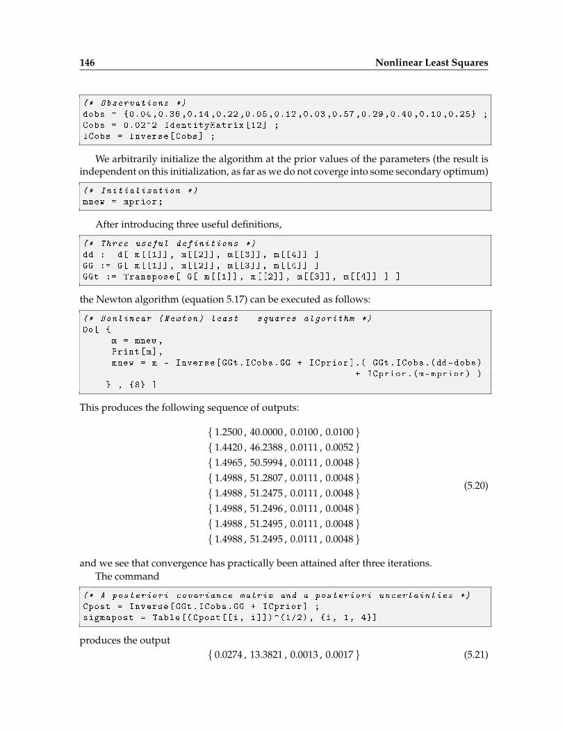
(* Observations *)

dobs = {0.04 ,0.36 ,0.14 ,0.22 ,0.05 ,0.12 ,0.03 ,0.57 ,0.29 ,0.40 ,0.10 ,0.25} ;

Cobs = 0.02^2 IdentityMatrix [12] ;

ICobs = Inverse[Cobs] ;

We arbitrarily initialize the algorithm at the prior values of the parameters (the result isindependent on this initialization, as far as we do not coverge into some secondary optimum)

(* Initialization *)

mnew = mprior;

After introducing three useful definitions,

(* Three useful definitions *)

dd := d[ m[[1]] , m[[2]] , m[[3]] , m[[4]] ]

GG := G[ m[[1]] , m[[2]] , m[[3]] , m[[4]] ]

GGt := Transpose[ G[ m[[1]], m[[2]] , m[[3]] , m[[4]] ] ]

the Newton algorithm (equation 5.17) can be executed as follows:

(* Nonlinear (Newton) least - squares algorithm *)

Do[ {

m = mnew ,

Print[m],

mnew = m - Inverse[GGt.ICobs.GG + ICprior ].( GGt.ICobs.(dd -dobs)

+ ICprior .(m-mprior) )

} , {8} ]

This produces the following sequence of outputs:

{ 1.2500 , 40.0000 , 0.0100 , 0.0100 }{ 1.4420 , 46.2388 , 0.0111 , 0.0052 }{ 1.4965 , 50.5994 , 0.0111 , 0.0048 }{ 1.4988 , 51.2807 , 0.0111 , 0.0048 }{ 1.4988 , 51.2475 , 0.0111 , 0.0048 }{ 1.4988 , 51.2496 , 0.0111 , 0.0048 }{ 1.4988 , 51.2495 , 0.0111 , 0.0048 }{ 1.4988 , 51.2495 , 0.0111 , 0.0048 }

(5.20)

and we see that convergence has practically been attained after three iterations.The command

(* A posteriori covariance matrix and a posteriori uncertainties *)

Cpost = Inverse[GGt.ICobs.GG + ICprior] ;

sigmapost = Table[( Cpost[[i, i]]) ^(1/2) , {i, 1, 4}]

produces the output{ 0.0274 , 13.3821 , 0.0013 , 0.0017 } (5.21)


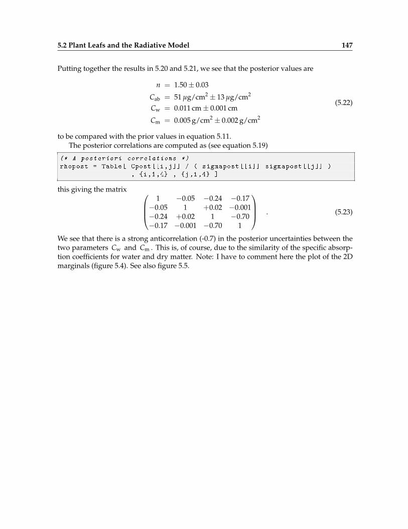
Putting together the results in 5.20 and 5.21, we see that the posterior values are

n = 1.50± 0.03


Cw = 0.011 cm± 0.001 cm

Cm = 0.005 g/cm2 ± 0.002 g/cm2

(5.22)

to be compared with the prior values in equation 5.11.The posterior correlations are computed as (see equation 5.19)

(* A posteriori correlations *)

rhopost = Table[ Cpost [[i,j]] / ( sigmapost [[i]] sigmapost [[j]] )

, {i,1,4} , {j,1,4} ]

this giving the matrix 1 −0.05 −0.24 −0.17

−0.05 1 +0.02 −0.001−0.24 +0.02 1 −0.70−0.17 −0.001 −0.70 1

. (5.23)

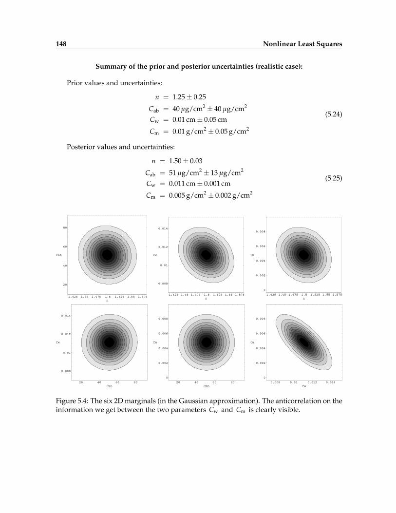
We see that there is a strong anticorrelation (-0.7) in the posterior uncertainties between thetwo parameters Cw and Cm . This is, of course, due to the similarity of the specific absorp-tion coefficients for water and dry matter. Note: I have to comment here the plot of the 2Dmarginals (figure 5.4). See also figure 5.5.


Summary of the prior and posterior uncertainties (realistic case):

Prior values and uncertainties:

n = 1.25± 0.25


Cw = 0.01 cm± 0.05 cm

Cm = 0.01 g/cm2 ± 0.05 g/cm2

(5.24)

Posterior values and uncertainties:

n = 1.50± 0.03


Cw = 0.011 cm± 0.001 cm

Cm = 0.005 g/cm2 ± 0.002 g/cm2

(5.25)

20 40 60 80Cab

0.008

0.01

0.012

0.014

Cw

1.425 1.45 1.475 1.5 1.525 1.55 1.575n

20

40

60

80

Cab

1.425 1.45 1.475 1.5 1.525 1.55 1.575n

0.008

0.01

0.012

0.014

Cw

0.008 0.01 0.012 0.014Cw

0

0.002

0.004

0.006

0.008

Cm

20 40 60 80Cab

0

0.002

0.004

0.006

0.008

Cm

1.425 1.45 1.475 1.5 1.525 1.55 1.575n

0

0.002

0.004

0.006

0.008

Cm

Figure 5.4: The six 2D marginals (in the Gaussian approximation). The anticorrelation on theinformation we get between the two parameters Cw and Cm is clearly visible.


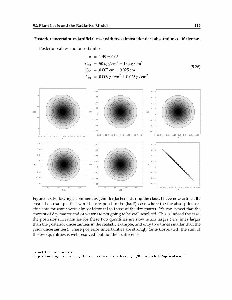
Posterior uncertainties (artificial case with two almost identical absorption coefficients):

Posterior values and uncertainties:

n = 1.49± 0.03


Cw = 0.007 cm± 0.025 cm

Cm = 0.009 g/cm2 ± 0.025 g/cm2

(5.26)

20 40 60 80Cab

-0.06

-0.04

-0.02

0

0.02

0.04

0.06

0.08

Cw

1.42 1.44 1.46 1.48 1.5 1.52 1.54 1.56n

20

40

60

80

Cab

1.42 1.44 1.46 1.48 1.5 1.52 1.54 1.56n

-0.06

-0.04

-0.02

0

0.02

0.04

0.06

0.08

Cw

20 40 60 80Cab

-0.06

-0.04

-0.02

0

0.02

0.04

0.06

0.08

Cm

1.42 1.44 1.46 1.48 1.5 1.52 1.54 1.56n

-0.06

-0.04

-0.02

0

0.02

0.04

0.06

0.08

Cm

-0.06-0.04-0.02 0 0.02 0.04 0.06 0.08Cw

-0.06

-0.04

-0.02

0

0.02

0.04

0.06

0.08

Cm

Figure 5.5: Following a comment by Jennifer Jackson during the class, I have now artificiallycreated an example that would correspond to the (bad!) case where the the absorption co-efficients for water were almost identical to those of the dry matter. We can expect that thecontent of dry matter and of water are not going to be well resolved. This is indeed the case:the posterior uncertainties for these two quantities are now much larger (ten times largerthan the posterior uncertainties in the realistic example, and only two times smaller than theprior uncertainties). These posterior uncertainties are strongly (anti-)correlated: the sum ofthe two quantities is well resolved, but not their difference.

Executable notebook at

http://www.ipgp.jussieu.fr/~tarantola/exercices/chapter_05/RadiativeWithDuplication.nb


5.2.3 Numerical Example (using Cartesian parameters)

Executable notebooks at

http://www.ipgp.jussieu.fr/~tarantola/exercices/chapter_05/RadiativeLog.nb

and

http://www.ipgp.jussieu.fr/~tarantola/exercices/chapter_05/RefractiveIndex.nb

Note: for the time being the mathematica code is not included here (see the files just men-tioned).

In relativity, the velocity v of a material particle has its velocity limited by the speed oflight, c , and it is well known that a useful parameter (that linearizes the rule of compositionof velocities) is

ψ = tanh-1 vc

. (5.27)

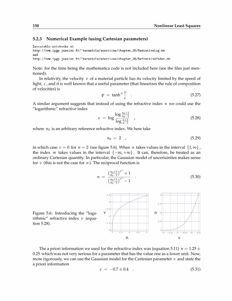
A similar argument suggests that instead of using the refractive index n we could use the“logarithmic” refractive index

ν = loglog n0+1

n0−1

log n+1n−1

, (5.28)

where n0 is an arbitrary reference refractive index. We here take

n0 = 2 , (5.29)

in which case ν = 0 for n = 2 (see figure 5.6). When n takes values in the interval {1, ∞} ,the index m takes values in the interval {−∞, +∞} . It can, therefore, be treated as anordinary Cartesian quantity. In particular, the Gaussian model of uncertainties makes sensefor ν (this is not the case for n ). The reciprocal function is

n =

( n0+1n0−1

)e-ν

+ 1( n0+1n0−1

)e-ν− 1

. (5.30)

Figure 5.6: Introducing the “loga-rithmic” refractive index ν (equa-tion 5.28).

n

ν

ν

n1 1.5 2 2.5 3

-2

-1.5

-1

-0.5

0

0.5

-2 -1.5 -1 -0.5 0 0.5

1

1.5

2

2.5

3

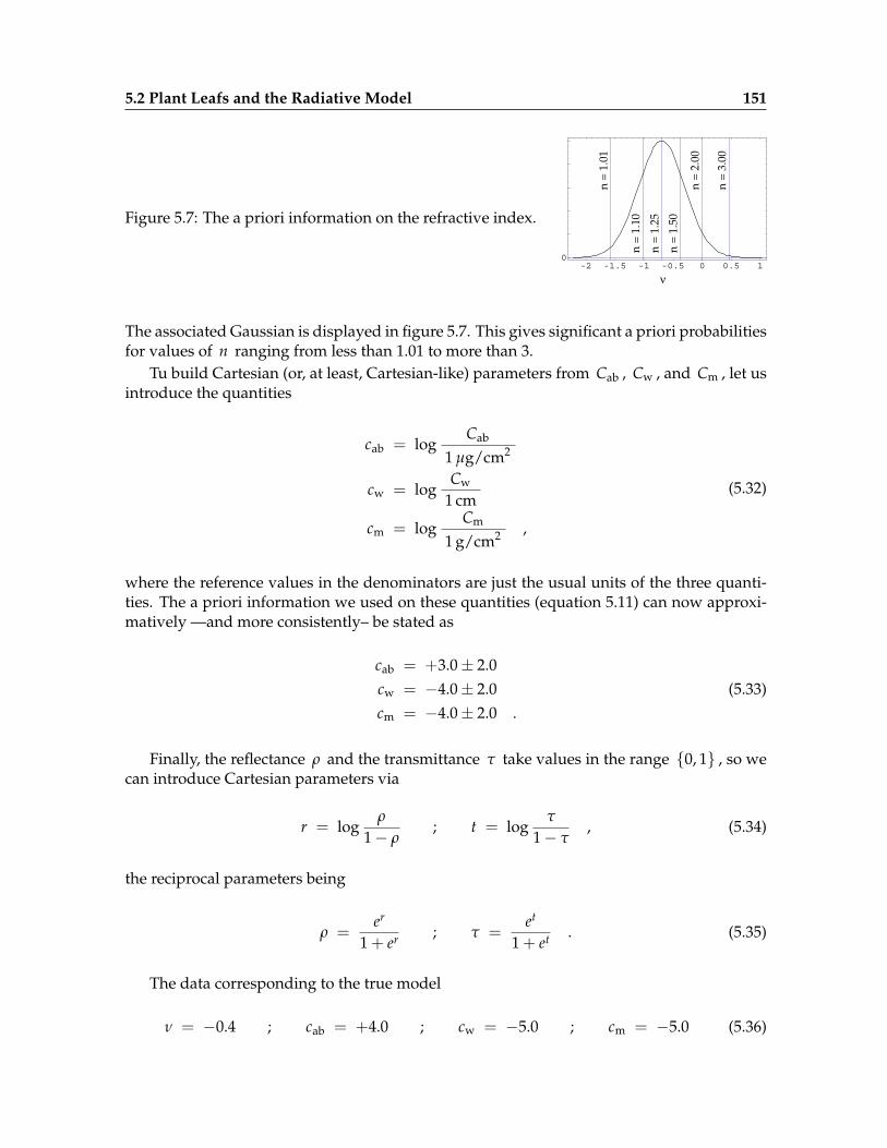
The a priori information we used for the refractive index was (equation 5.11) n = 1.25±0.25 which was not very serious for a parameter that has the value one as a lower unit. Now,more rigorously, we can use the Gaussian model for the Cartesian parameter ν and state thea priori information

ν = −0.7± 0.4 . (5.31)


Figure 5.7: The a priori information on the refractive index.

-2 -1.5 -1 -0.5 0 0.5 10

n =

1.01

n =

1.10

n =

1.25

n =

1.50

n =

3.00

n =

2.00

!

The associated Gaussian is displayed in figure 5.7. This gives significant a priori probabilitiesfor values of n ranging from less than 1.01 to more than 3.

Tu build Cartesian (or, at least, Cartesian-like) parameters from Cab , Cw , and Cm , let usintroduce the quantities

cab = logCab

1 µg/cm2

cw = logCw

1 cm

cm = logCm

1 g/cm2 ,

(5.32)

where the reference values in the denominators are just the usual units of the three quanti-ties. The a priori information we used on these quantities (equation 5.11) can now approxi-matively —and more consistently– be stated as

cab = +3.0± 2.0cw = −4.0± 2.0cm = −4.0± 2.0 .

(5.33)

Finally, the reflectance ρ and the transmittance τ take values in the range {0, 1} , so wecan introduce Cartesian parameters via

r = logρ

1− ρ; t = log

τ

1− τ, (5.34)

the reciprocal parameters being

ρ =er

1 + er ; τ =et

1 + et . (5.35)

The data corresponding to the true model

ν = −0.4 ; cab = +4.0 ; cw = −5.0 ; cm = −5.0 (5.36)


are (with rounding errors, and the corresponding uncertainties assumed)

r(λ1) = −3.2± 0.2 ; t(λ1) = −3.5± 0.2r(λ2) = −0.6± 0.2 ; t(λ2) = +0.3± 0.2r(λ3) = −1.5± 0.2 ; t(λ3) = −0.6± 0.2r(λ4) = −1.2± 0.2 ; t(λ4) = −0.3± 0.2r(λ5) = −2.5± 0.2 ; t(λ5) = −1.6± 0.2r(λ6) = −1.9± 0.2 ; t(λ6) = −1.0± 0.2 .

(5.37)

Using the algorithm introduced in the previous section (but the partial derivatives cor-responding to the new parameters) gives the posterior values (see the second mathematicanotebook)

ν = −0.39± 0.04cab = +3.98± 0.09cw = −5.04± 0.16cm = −4.95± 0.30 .

(5.38)

All the posterior correlations are small, excepted that associated to cw and cm whose valueis -0.7 . As mentioned above, this is due to the similarity of the specific absorption coefficientsfor water and dry matter.

5.2.4 Bibliography

Allen W.A., Gausman H.W., Richardson A.J., and Thomas J.R., 1969, Interaction of isotropiclight with a compact plant leaf, Journal of the Optical Society of America, 59(10), p. 1376–1379.

Sinclair, T.R., Schreiber, M.M., and Hoffer, R.M., 1973, Diffuse reflectance hypothesis for thepathway of Solar radiation through leaves, Agronomy Journal, 65, p. 276–283.

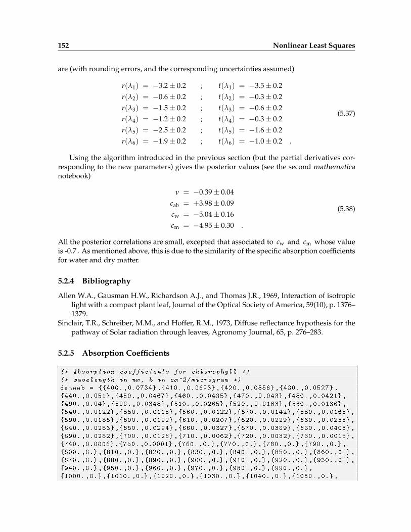
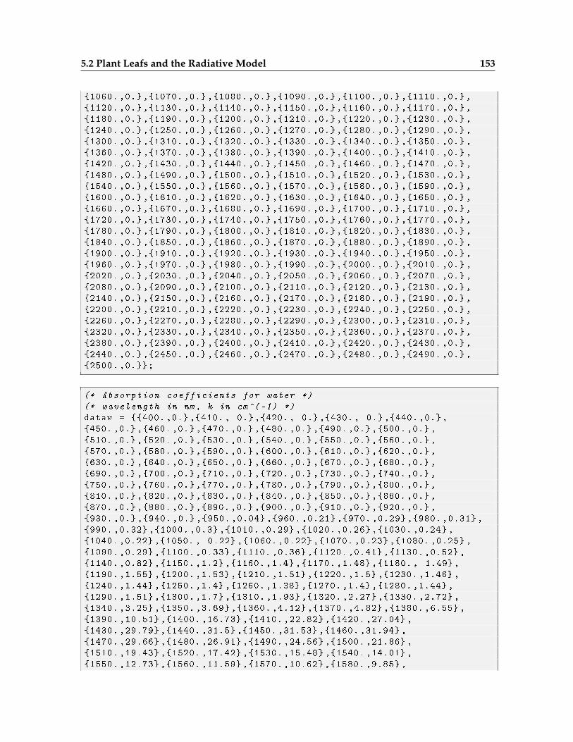
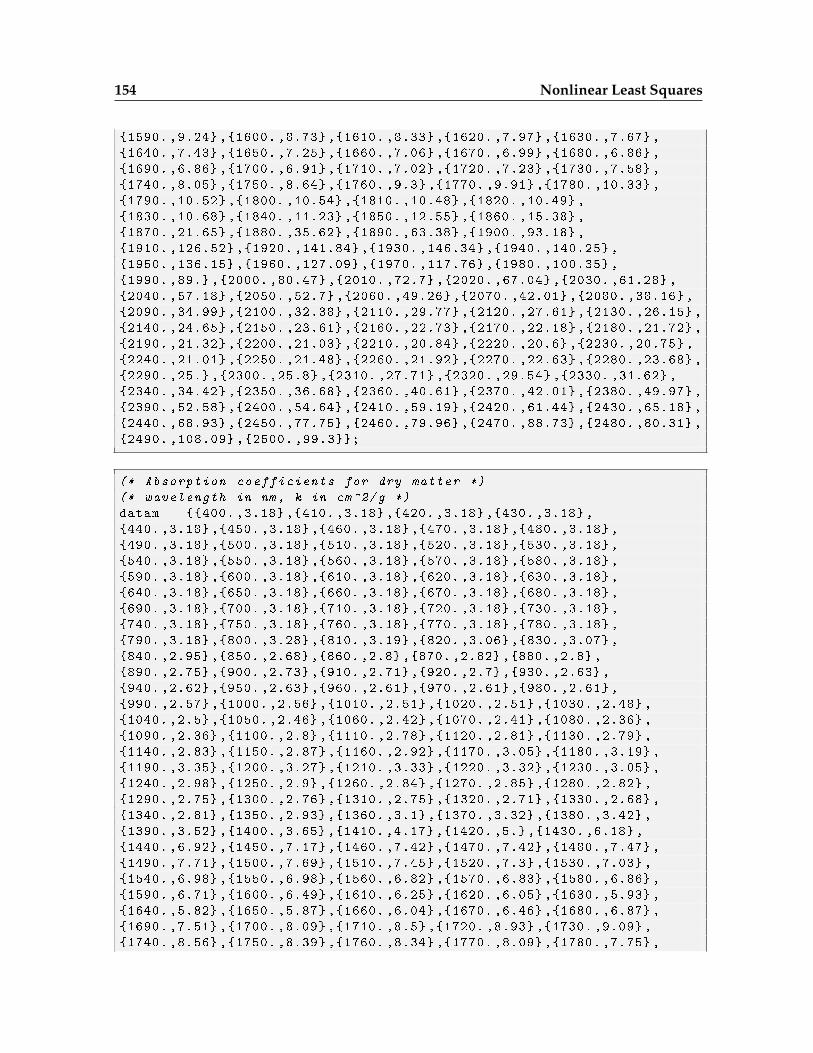
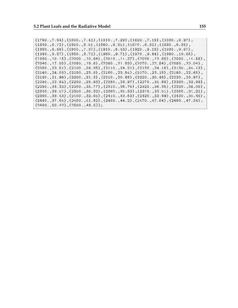
5.2.5 Absorption Coefficients

(* Absorption coefficients for chlorophyll *)

(* wavelength in nm, k in cm^2/ microgram *)

dataab = {{400. ,0.0734} ,{410. ,0.0623} ,{420. ,0.0556} ,{430. ,0.0527} ,

{440. ,0.051} ,{450. ,0.0467} ,{460. ,0.0435} ,{470. ,0.043} ,{480. ,0.0421} ,

{490. ,0.04} ,{500. ,0.0348} ,{510. ,0.0265} ,{520. ,0.0183} ,{530. ,0.0136} ,

{540. ,0.0122} ,{550. ,0.0118} ,{560. ,0.0122} ,{570. ,0.0142} ,{580. ,0.0168} ,

{590. ,0.0185} ,{600. ,0.0192} ,{610. ,0.0207} ,{620. ,0.0229} ,{630. ,0.0236} ,

{640. ,0.0253} ,{650. ,0.0294} ,{660. ,0.0327} ,{670. ,0.0389} ,{680. ,0.0403} ,

{690. ,0.0282} ,{700. ,0.0126} ,{710. ,0.0062} ,{720. ,0.0032} ,{730. ,0.0015} ,

{740. ,0.0006} ,{750. ,0.0001} ,{760. ,0.} ,{770. ,0.} ,{780. ,0.} ,{790. ,0.} ,

{800. ,0.} ,{810. ,0.} ,{820. ,0.} ,{830. ,0.} ,{840. ,0.} ,{850. ,0.} ,{860. ,0.} ,

{870. ,0.} ,{880. ,0.} ,{890. ,0.} ,{900. ,0.} ,{910. ,0.} ,{920. ,0.} ,{930. ,0.} ,

{940. ,0.} ,{950. ,0.} ,{960. ,0.} ,{970. ,0.} ,{980. ,0.} ,{990. ,0.} ,

{1000. ,0.} ,{1010. ,0.} ,{1020. ,0.} ,{1030. ,0.} ,{1040. ,0.} ,{1050. ,0.} ,


{1060. ,0.} ,{1070. ,0.} ,{1080. ,0.} ,{1090. ,0.} ,{1100. ,0.} ,{1110. ,0.} ,

{1120. ,0.} ,{1130. ,0.} ,{1140. ,0.} ,{1150. ,0.} ,{1160. ,0.} ,{1170. ,0.} ,

{1180. ,0.} ,{1190. ,0.} ,{1200. ,0.} ,{1210. ,0.} ,{1220. ,0.} ,{1230. ,0.} ,

{1240. ,0.} ,{1250. ,0.} ,{1260. ,0.} ,{1270. ,0.} ,{1280. ,0.} ,{1290. ,0.} ,

{1300. ,0.} ,{1310. ,0.} ,{1320. ,0.} ,{1330. ,0.} ,{1340. ,0.} ,{1350. ,0.} ,

{1360. ,0.} ,{1370. ,0.} ,{1380. ,0.} ,{1390. ,0.} ,{1400. ,0.} ,{1410. ,0.} ,

{1420. ,0.} ,{1430. ,0.} ,{1440. ,0.} ,{1450. ,0.} ,{1460. ,0.} ,{1470. ,0.} ,

{1480. ,0.} ,{1490. ,0.} ,{1500. ,0.} ,{1510. ,0.} ,{1520. ,0.} ,{1530. ,0.} ,

{1540. ,0.} ,{1550. ,0.} ,{1560. ,0.} ,{1570. ,0.} ,{1580. ,0.} ,{1590. ,0.} ,

{1600. ,0.} ,{1610. ,0.} ,{1620. ,0.} ,{1630. ,0.} ,{1640. ,0.} ,{1650. ,0.} ,

{1660. ,0.} ,{1670. ,0.} ,{1680. ,0.} ,{1690. ,0.} ,{1700. ,0.} ,{1710. ,0.} ,

{1720. ,0.} ,{1730. ,0.} ,{1740. ,0.} ,{1750. ,0.} ,{1760. ,0.} ,{1770. ,0.} ,

{1780. ,0.} ,{1790. ,0.} ,{1800. ,0.} ,{1810. ,0.} ,{1820. ,0.} ,{1830. ,0.} ,

{1840. ,0.} ,{1850. ,0.} ,{1860. ,0.} ,{1870. ,0.} ,{1880. ,0.} ,{1890. ,0.} ,

{1900. ,0.} ,{1910. ,0.} ,{1920. ,0.} ,{1930. ,0.} ,{1940. ,0.} ,{1950. ,0.} ,

{1960. ,0.} ,{1970. ,0.} ,{1980. ,0.} ,{1990. ,0.} ,{2000. ,0.} ,{2010. ,0.} ,

{2020. ,0.} ,{2030. ,0.} ,{2040. ,0.} ,{2050. ,0.} ,{2060. ,0.} ,{2070. ,0.} ,

{2080. ,0.} ,{2090. ,0.} ,{2100. ,0.} ,{2110. ,0.} ,{2120. ,0.} ,{2130. ,0.} ,

{2140. ,0.} ,{2150. ,0.} ,{2160. ,0.} ,{2170. ,0.} ,{2180. ,0.} ,{2190. ,0.} ,

{2200. ,0.} ,{2210. ,0.} ,{2220. ,0.} ,{2230. ,0.} ,{2240. ,0.} ,{2250. ,0.} ,

{2260. ,0.} ,{2270. ,0.} ,{2280. ,0.} ,{2290. ,0.} ,{2300. ,0.} ,{2310. ,0.} ,

{2320. ,0.} ,{2330. ,0.} ,{2340. ,0.} ,{2350. ,0.} ,{2360. ,0.} ,{2370. ,0.} ,

{2380. ,0.} ,{2390. ,0.} ,{2400. ,0.} ,{2410. ,0.} ,{2420. ,0.} ,{2430. ,0.} ,

{2440. ,0.} ,{2450. ,0.} ,{2460. ,0.} ,{2470. ,0.} ,{2480. ,0.} ,{2490. ,0.} ,

{2500. ,0.}};

(* Absorption coefficients for water *)

(* wavelength in nm, k in cm^(-1) *)

dataw = {{400. ,0.} ,{410. , 0.} ,{420. , 0.} ,{430. , 0.} ,{440. ,0.} ,

{450. ,0.} ,{460. ,0.} ,{470. ,0.} ,{480. ,0.} ,{490. ,0.} ,{500. ,0.} ,

{510. ,0.} ,{520. ,0.} ,{530. ,0.} ,{540. ,0.} ,{550. ,0.} ,{560. ,0.} ,

{570. ,0.} ,{580. ,0.} ,{590. ,0.} ,{600. ,0.} ,{610. ,0.} ,{620. ,0.} ,

{630. ,0.} ,{640. ,0.} ,{650. ,0.} ,{660. ,0.} ,{670. ,0.} ,{680. ,0.} ,

{690. ,0.} ,{700. ,0.} ,{710. ,0.} ,{720. ,0.} ,{730. ,0.} ,{740. ,0.} ,

{750. ,0.} ,{760. ,0.} ,{770. ,0.} ,{780. ,0.} ,{790. ,0.} ,{800. ,0.} ,

{810. ,0.} ,{820. ,0.} ,{830. ,0.} ,{840. ,0.} ,{850. ,0.} ,{860. ,0.} ,

{870. ,0.} ,{880. ,0.} ,{890. ,0.} ,{900. ,0.} ,{910. ,0.} ,{920. ,0.} ,

{930. ,0.} ,{940. ,0.} ,{950. ,0.04} ,{960. ,0.21} ,{970. ,0.29} ,{980. ,0.31} ,

{990. ,0.32} ,{1000. ,0.3} ,{1010. ,0.29} ,{1020. ,0.26} ,{1030. ,0.24} ,

{1040. ,0.22} ,{1050. , 0.22} ,{1060. ,0.22} ,{1070. ,0.23} ,{1080. ,0.25} ,

{1090. ,0.29} ,{1100. ,0.33} ,{1110. ,0.36} ,{1120. ,0.41} ,{1130. ,0.52} ,

{1140. ,0.82} ,{1150. ,1.2} ,{1160. ,1.4} ,{1170. ,1.48} ,{1180. , 1.49},

{1190. ,1.55} ,{1200. ,1.53} ,{1210. ,1.51} ,{1220. ,1.5} ,{1230. ,1.46} ,

{1240. ,1.44} ,{1250. ,1.4} ,{1260. ,1.38} ,{1270. ,1.4} ,{1280. ,1.44} ,

{1290. ,1.51} ,{1300. ,1.7} ,{1310. ,1.93} ,{1320. ,2.27} ,{1330. ,2.72} ,

{1340. ,3.25} ,{1350. ,3.69} ,{1360. ,4.12} ,{1370. ,4.82} ,{1380. ,6.55} ,

{1390. ,10.51} ,{1400. ,16.73} ,{1410. ,22.82} ,{1420. ,27.04} ,

{1430. ,29.79} ,{1440. ,31.5} ,{1450. ,31.53} ,{1460. ,31.94} ,

{1470. ,29.66} ,{1480. ,26.91} ,{1490. ,24.56} ,{1500. ,21.86} ,

{1510. ,19.43} ,{1520. ,17.42} ,{1530. ,15.48} ,{1540. ,14.01} ,

{1550. ,12.73} ,{1560. ,11.59} ,{1570. ,10.62} ,{1580. ,9.85} ,


{1590. ,9.24} ,{1600. ,8.73} ,{1610. ,8.33} ,{1620. ,7.97} ,{1630. ,7.67} ,

{1640. ,7.43} ,{1650. ,7.25} ,{1660. ,7.06} ,{1670. ,6.99} ,{1680. ,6.86} ,

{1690. ,6.86} ,{1700. ,6.91} ,{1710. ,7.02} ,{1720. ,7.23} ,{1730. ,7.58} ,

{1740. ,8.05} ,{1750. ,8.64} ,{1760. ,9.3} ,{1770. ,9.91} ,{1780. ,10.33} ,

{1790. ,10.52} ,{1800. ,10.54} ,{1810. ,10.48} ,{1820. ,10.49} ,

{1830. ,10.68} ,{1840. ,11.23} ,{1850. ,12.55} ,{1860. ,15.38} ,

{1870. ,21.65} ,{1880. ,35.62} ,{1890. ,63.38} ,{1900. ,93.18} ,

{1910. ,126.52} ,{1920. ,141.84} ,{1930. ,146.34} ,{1940. ,140.25} ,

{1950. ,136.15} ,{1960. ,127.09} ,{1970. ,117.76} ,{1980. ,100.35} ,

{1990. ,89.} ,{2000. ,80.47} ,{2010. ,72.7} ,{2020. ,67.04} ,{2030. ,61.28} ,

{2040. ,57.18} ,{2050. ,52.7} ,{2060. ,49.26} ,{2070. ,42.01} ,{2080. ,38.16} ,

{2090. ,34.99} ,{2100. ,32.38} ,{2110. ,29.77} ,{2120. ,27.61} ,{2130. ,26.15} ,

{2140. ,24.65} ,{2150. ,23.61} ,{2160. ,22.73} ,{2170. ,22.18} ,{2180. ,21.72} ,

{2190. ,21.32} ,{2200. ,21.03} ,{2210. ,20.84} ,{2220. ,20.6} ,{2230. ,20.75} ,

{2240. ,21.01} ,{2250. ,21.48} ,{2260. ,21.92} ,{2270. ,22.63} ,{2280. ,23.68} ,

{2290. ,25.} ,{2300. ,25.8} ,{2310. ,27.71} ,{2320. ,29.54} ,{2330. ,31.62} ,

{2340. ,34.42} ,{2350. ,36.68} ,{2360. ,40.61} ,{2370. ,42.01} ,{2380. ,49.97} ,

{2390. ,52.58} ,{2400. ,54.64} ,{2410. ,59.19} ,{2420. ,61.44} ,{2430. ,65.18} ,

{2440. ,68.93} ,{2450. ,77.75} ,{2460. ,79.96} ,{2470. ,88.73} ,{2480. ,80.31} ,

{2490. ,108.09} ,{2500. ,99.3}};

(* Absorption coefficients for dry matter *)

(* wavelength in nm, k in cm^2/g *)

datam = {{400. ,3.18} ,{410. ,3.18} ,{420. ,3.18} ,{430. ,3.18} ,

{440. ,3.18} ,{450. ,3.18} ,{460. ,3.18} ,{470. ,3.18} ,{480. ,3.18} ,

{490. ,3.18} ,{500. ,3.18} ,{510. ,3.18} ,{520. ,3.18} ,{530. ,3.18} ,

{540. ,3.18} ,{550. ,3.18} ,{560. ,3.18} ,{570. ,3.18} ,{580. ,3.18} ,

{590. ,3.18} ,{600. ,3.18} ,{610. ,3.18} ,{620. ,3.18} ,{630. ,3.18} ,

{640. ,3.18} ,{650. ,3.18} ,{660. ,3.18} ,{670. ,3.18} ,{680. ,3.18} ,

{690. ,3.18} ,{700. ,3.18} ,{710. ,3.18} ,{720. ,3.18} ,{730. ,3.18} ,

{740. ,3.18} ,{750. ,3.18} ,{760. ,3.18} ,{770. ,3.18} ,{780. ,3.18} ,

{790. ,3.18} ,{800. ,3.28} ,{810. ,3.19} ,{820. ,3.06} ,{830. ,3.07} ,

{840. ,2.95} ,{850. ,2.68} ,{860. ,2.8} ,{870. ,2.82} ,{880. ,2.8} ,

{890. ,2.75} ,{900. ,2.73} ,{910. ,2.71} ,{920. ,2.7} ,{930. ,2.63} ,

{940. ,2.62} ,{950. ,2.63} ,{960. ,2.61} ,{970. ,2.61} ,{980. ,2.61} ,

{990. ,2.57} ,{1000. ,2.56} ,{1010. ,2.51} ,{1020. ,2.51} ,{1030. ,2.48} ,

{1040. ,2.5} ,{1050. ,2.46} ,{1060. ,2.42} ,{1070. ,2.41} ,{1080. ,2.36} ,

{1090. ,2.36} ,{1100. ,2.8} ,{1110. ,2.78} ,{1120. ,2.81} ,{1130. ,2.79} ,

{1140. ,2.83} ,{1150. ,2.87} ,{1160. ,2.92} ,{1170. ,3.05} ,{1180. ,3.19} ,

{1190. ,3.35} ,{1200. ,3.27} ,{1210. ,3.33} ,{1220. ,3.32} ,{1230. ,3.05} ,

{1240. ,2.98} ,{1250. ,2.9} ,{1260. ,2.84} ,{1270. ,2.85} ,{1280. ,2.82} ,

{1290. ,2.75} ,{1300. ,2.76} ,{1310. ,2.75} ,{1320. ,2.71} ,{1330. ,2.68} ,

{1340. ,2.81} ,{1350. ,2.93} ,{1360. ,3.1} ,{1370. ,3.32} ,{1380. ,3.42} ,

{1390. ,3.52} ,{1400. ,3.65} ,{1410. ,4.17} ,{1420. ,5.} ,{1430. ,6.18} ,

{1440. ,6.92} ,{1450. ,7.17} ,{1460. ,7.42} ,{1470. ,7.42} ,{1480. ,7.47} ,

{1490. ,7.71} ,{1500. ,7.69} ,{1510. ,7.45} ,{1520. ,7.3} ,{1530. ,7.03} ,

{1540. ,6.98} ,{1550. ,6.98} ,{1560. ,6.82} ,{1570. ,6.83} ,{1580. ,6.86} ,

{1590. ,6.71} ,{1600. ,6.49} ,{1610. ,6.25} ,{1620. ,6.05} ,{1630. ,5.93} ,

{1640. ,5.82} ,{1650. ,5.87} ,{1660. ,6.04} ,{1670. ,6.46} ,{1680. ,6.87} ,

{1690. ,7.51} ,{1700. ,8.09} ,{1710. ,8.5} ,{1720. ,8.93} ,{1730. ,9.09} ,

{1740. ,8.56} ,{1750. ,8.39} ,{1760. ,8.34} ,{1770. ,8.09} ,{1780. ,7.75} ,


{1790. ,7.54} ,{1800. ,7.41} ,{1810. ,7.29} ,{1820. ,7.19} ,{1830. ,6.97} ,

{1840. ,6.72} ,{1850. ,6.5} ,{1860. ,6.35} ,{1870. ,6.31} ,{1880. ,6.36} ,

{1890. ,6.69} ,{1900. ,7.37} ,{1910. ,8.43} ,{1920. ,9.18} ,{1930. ,9.67} ,

{1940. ,9.57} ,{1950. ,9.71} ,{1960. ,9.71} ,{1970. ,9.84} ,{1980. ,10.05} ,

{1990. ,10.15} ,{2000. ,10.64} ,{2010. ,11.37} ,{2020. ,12.66} ,{2030. ,14.56} ,

{2040. ,17.05} ,{2050. ,19.6} ,{2060. ,21.59} ,{2070. ,22.54} ,{2080. ,23.04} ,

{2090. ,23.51} ,{2100. ,24.05} ,{2110. ,24.21} ,{2120. ,24.16} ,{2130. ,24.13} ,

{2140. ,24.05} ,{2150. ,23.9} ,{2160. ,23.54} ,{2170. ,23.15} ,{2180. ,22.65} ,

{2190. ,21.96} ,{2200. ,21.3} ,{2210. ,20.88} ,{2220. ,20.48} ,{2230. ,20.97} ,

{2240. ,22.84} ,{2250. ,25.93} ,{2260. ,28.97} ,{2270. ,31.56} ,{2280. ,32.99} ,

{2290. ,34.33} ,{2300. ,35.77} ,{2310. ,36.76} ,{2320. ,36.35} ,{2330. ,36.05} ,

{2340. ,36.57} ,{2350. ,36.32} ,{2360. ,35.83} ,{2370. ,34.51} ,{2380. ,34.21} ,

{2390. ,33.43} ,{2400. ,32.65} ,{2410. ,33.63} ,{2420. ,33.99} ,{2430. ,35.46} ,

{2440. ,37.64} ,{2450. ,41.82} ,{2460. ,44.2} ,{2470. ,47.04} ,{2480. ,47.34} ,

{2490. ,50.42} ,{2500. ,48.5}};

Documents

Inverse Problems: Exercices - Jussieutarantola/exercices/chapter_05/Radiative.pdf · Individual Sections of the Book Inverse Problems: Exercices With mathematica, matlab, and scilab