Embed Size (px)
Citation preview

1
Inverse modeling of methane sources and sinks using the adjoint of aglobal transport model
Sander Houweling, 1 Thomas Kaminski, 2 Frank Dentener, 1 Jos Lelieveld, 1 and Martin
Heimann3
Short title: INVERSE MODELING OF METHANE
1Institute for Marine and Atmospheric Research Utrecht (IMAU), Utrecht University, The
Netherlands.
2Max Planck Insitute of Meteorology, Hamburg, Germany.
3Max Planck Insitute of Bio Geo-chemical Cycles, Jena, Germany.

2
Abstract. An inverse modeling method is presented to evaluate the sources and sinks
of atmospheric methane. An adjoint version of a global transport model has been used to
estimate these fluxes at a relatively high spatial and temporal resolution. Measurements from
34 monitoring stations and 11 locations along two ship cruises by the National Oceanographic
and Atmospheric Administration have been used as input. Recent estimates of methane
sources, including a number of minor ones, have been used as a priori constraints. For the
target period 1993–1995 our inversion reduces the a priori assumed global methane emissions
of 528 to 505 Tg(CH4) yr−1 a posteriori. Further, the relative contribution of the Northern
Hemispheric sources decreases from 77% a priori to 67% a posteriori. In addition to making
the emission estimate more consistent with the measurements, the inversion helps to reduce
the uncertainties in the sources. Uncertainty reductions vary from 75% on the global scale to
∼1% on the grid-scale (8◦x10◦), indicating that the grid scale variability is not resolved by
the measurements. Large scale features such as the interhemispheric methane concentration
gradient are relatively well resolved and therefore impose strong constraints on the estimated
fluxes. The capability of the model to reproduce this gradient is critically dependent on the
accuracy at which the interhemispheric tracer exchange and the large-scale hydroxyl radical
distribution are represented. As a consequence, the inversion-derived emission estimates are
sensitive to errors in the transport model and the calculated hydroxyl radical distribution. In
fact, a considerable contribution of these model errors cannot be ignored. This underscores
that source quantification by inverse modeling is limited by the extent to which the rate of
interhemispheric transport and the hydroxyl radical distribution can be validated. We show
that the use of temporal and spatial correlations of emissions may significantly improve our
results; however, at present the experimental support for such correlations is lacking. Our
results further indicate that uncertainty reductions reported in previous inverse studies of
methane have been overestimated.

3
1. Introduction
Our understanding of atmospheric methane is to a large extent limited by a poor
quantification of its sources. Although the dominant methane-producing processes seem to
be identified, their global distributions as well as globally integrated source strengths are
still highly uncertain. Some sources for which relatively reliable statistics exist, for instance,
emissions by domestic ruminants, are relatively well constrained by integrating or scaling-up
the sources. For sources that have a large natural variability, for example, emissions from rice
paddies and natural wetlands, the opposite is true. Despite considerable effort to constrain
these important sources, progress is slow. For example, the amount of methane released from
rice paddies has recently been estimated at 80 ±50 Tg(CH4) yr−1 [Lelieveld et al., 1998],
indicating an uncertainty range similar to the IPCC [1990] estimate of nearly a decade ago
(20–150 Tg(CH4)/yr). Recent estimates of global methane emissions from natural wetlands,
the largest single source of methane, by Lelieveld et al. [1998] and Hein et al. [1997] disagree
strangely (145 ±30 and 232 ±27 Tg(CH4) yr−1, respectively).
Measurements over the past decade show a significant variability of the globally averaged
methane trend. The fluctuations in the early 1990s have been merely attributed to the
Mount Pinatubo eruption, but the underlying processes remain unclear [Dlugokencky et al.,
1994a, 1996]. Recent measurements indicate that the methane trend continues to decline
[Dlugokencky et al., 1998]. For the changes observed so far the sources and sinks of methane
are not well enough constrained to provide a reliable explanation. As a consequence, the
foundation for any future scenario of methane in the atmosphere is weak. It is important to
improve our understanding of the atmospheric budget of methane since it plays an important
role in radiative and chemical balances in the atmosphere.
In addition to upscaling techniques, inverse modeling can be used to estimate sources.
This method makes use of measurements of trace gas concentrations, which are translated to
constraints on the sources by means of an atmospheric transport model. Generally, the number
of available measurements is a limiting factor in this approach. For such an inverse problem
4
to have a single solution either the number of emission parameters to be estimated must be
adjusted according to the available measurements, or different constraints must be introduced.
Often it is required that the solution be close to existing knowledge by introducing first guess
or a priori information of the sources. This can be done in a consistent way by adopting a
so-called Bayesian approach, in which all parameters are expressed as statistical probability
distributions. A solution in the form of a superposition of all statistical distributions involved
can be computed, from which means and covariances can be derived.
Until now a number of studies have quantified global-scale sources using inverse
methods aiming at different trace gases, such as CFCs [Brown, 1993; Hartley and Prinn,
1993; Plumb and Zheng, 1996; Mulquiney and Norton, 1998; Mulquiney et al., 1998], CH4
[Brown, 1993, 1995; Hein et al., 1997], CO2 [Enting et al., 1995; Rayner et al., 1996; Law
and Simmonds, 1996; Kaminski et al., 1999b]. In all these studies except the last, fluxes
are aggregated into a few large regions. This “big region” approach has the disadvantage
that emission distributions over predefined regions are assumed to be perfectly well known,
which, in practice, is justified by computational limitations rather than by knowledge about
the sources. In fact, such an approach may lead to significant biases in the estimated emissions
caused by nonhomogeneous sampling by the measurement network as shown by Trampert
and Snieder [1996]. Presently, it is unknown at which resolution fluxes should be represented
in order to reduce this bias to an insignificant size. Sensitivity studies, however, show that
significant biases occur when continental-scale regions are applied (T. Kaminski, personal
communication, 1998).
The aim of this paper is to study the sources and sinks of methane on a global scale and to
assess the usefulness of the existing measurement data as constraints. In this study, as opposed
to previous studies, biases are minimized using the method of Kaminski et al. [1999a]. To
compute efficiently the large number of sensitivities needed to perform an inversion in this
approach, an adjoint model is used. Except for the definition of the fluxes and the method
to derive the sensitivities the method we adopt resembles the method by Hein et al. [1997].

5
Compared with this study, the measurements and first-guess assumptions have been extended
and updated.
Using our method, the inverse problem is strongly underdetermined because of the large
increase in the number of unknown compared with Hein et al. [1997], whereas the number
of constraints (measurements) is about the same. This can be interpreted as a reduction of a
priori information since temporal and spatial distributions of the sources and sinks within the
regions are no longer assumed to be well known. In fact, we choose the opposite starting point
by assuming that the uncertainties in the fluxes are fully uncorrelated. From this viewpoint the
big region approach can be considered as a case in which all fluxes over a region are assumed
to be fully correlated. Hence our confidence in the a priori emission distributions can be
expressed in the spatial and temporal correlation of source and sink uncertainties. Our method
allows different scenarios for treating these correlations.
In the next section the inverse modeling technique will be explained. We describe the
model in section 3, a priori knowledge on sources and sinks and measurements in sections 4
and 5, and the relevant chemistry in section 6. In section 7 the results of the methane inversion
are presented, focusing on differences between a priori and a posteriori estimates. The impact
of correlated uncertainties is studied in section 8, where we also present results using different
scenarios. Sensitivity tests have been performed to investigate the potential influence of the
major assumptions on the estimated sources and sinks. Finally, the ability of this method to
solve questions related to different emissions scenarios has been studied with rice paddies as a
test case in section 9.
2. Inversion Method and Unknowns
To deduce information about surface emissions from measured concentrations, we
use a global atmospheric chemistry transport model (CTM) that relates these emissions to
concentrations. In mathematical terminology the CTM defines a mapping (or function) of a
parameter set (including the emissions) on the simulated concentrations. For any measured

6
methane concentration di,t at location i and month t this function can be written in the form
di,t = di,t[f,Q(f,sOH,sstra,c0),R(f,soh,sstra,c0),c0], (1)
where any component f j,m of the vector f represents the integrated surface emission over
region j and month m. Since f j,m may either represent a surface source or sink, in the following
the term “flux” will be used to denote exchange between the surface and the atmosphere. The
sOH parameterizes the chemical removal of methane Q due to the reaction with the hydroxyl
radical in each tropospheric grid box. Similarly, sstra and R refer to stratospheric methane loss
as a result of the reactions with O(1D), Cl, Br, OH radicals, and methane photolysis. Finally,
c0 is defined as the global mean methane concentration at the start of a simulation. The aim
of the inversion is to find the set of most probable values for the parameters f, sOH , sstra, and
c0. For this purpose we iteratively apply a linear inversion procedure that combines the set of
observations d and a set of a priori estimates f, sOH , sstra, and c0 using (1).
We need to iterate because the chemistry introduces a nonlinearity as explained below.
The amount of methane Qk,l oxidized by hydroxyl radicals in a particular tropospheric grid
box k and month l can be represented as
Qk,l = sOHkOH(T )[OH]k,l[CH4]k,l, (2)
where kOH is the temperature-dependent rate constant for the reaction between the hydroxyl
radical and methane. The dependency of the amount of methane oxidized on its concentration
[CH4]k,l causes a nonlinear response to the fluxes at the observational sites. Since tropospheric
methane oxidation influences the hydroxyl radical concentration, there is also a feedback
mechanism through changes of [OH]k,l. Similar nonlinearities occur because of the
stratospheric sink.
Different strategies can be adopted to define the fluxes represented by the parameters
f j,m. One approach is to classify fluxes geographically, for example, per continent or country
[see, e.g., Hartley and Prinn [1993]; Mulquiney et al. [1998]]. Alternatively, a classification

7
distinguishing different flux-producing processes can be used, as is done, for instance, by Hein
et al. [1997]. Unless both the emission distributions over the specified regions and the model
are perfect, non homogeneous sampling by the sparse network will lead to biased emission
estimates [Trampert and Snieder, 1996]. This bias can be reduced by decreasing the size of the
regions or by defining the regions such that the uncertainty in the flux distribution over each
region is minimal. Because of the large spatial variability of CH4 emissions, we lack such
well-defined regions. Therefore, over the continents we choose to represent the surface flux in
every continental surface grid box of our CTM by a separate flux parameter. In contrast, ocean
grid boxes without linkages to continents or continental shelfs are aggregated into one single
region. For all fluxes, including those from the oceans, a temporal resolution of 1 month is
used; hence seasonal cycles are also subject to optimization.
The open ocean source is mainly driven by a small methane supersaturation in the surface
layer, ranging from 0.95 to 1.17 over the oceans [Bates et al., 1996]. Although the methane
concentration in ocean water has been determined at a limited number of sites only, the
available data suggest that the net emission is only small and that the variability is not large
enough to influence significantly the atmospheric methane concentration distribution. The
north and south polar ice shields are treated similarly to the oceans, which is justified by the
absence of any known significant surface source or sink in these regions. As a result of both
flux aggregations, the total number of surface flux parameters is reduced by about a factor of
2.
In (2) we scale the amount of methane oxidized in every tropospheric grid box by a single
parameter sOH , which implies that the entire spatiotemporal distribution of the OH radical
field is kept constant. Unlike the ocean and polar sources, such a treatment of the OH sink is
not sustained by our knowledge of the tropospheric OH distribution. Treating the OH sink this
way is equivalent to assuming that the OH distribution is perfectly known, which is not the
case. In fact, we lack the tools to validate model-simulated OH distributions for aspects other
than large-scale averages. The fact that other reactive trace gases, such as carbon monoxide

8
and ozone, are simulated realistically by our model [Houweling et al., 1998] indicates,
however, that the large-scale chemistry and transport are adequately represented. Therefore
we fix the OH distribution, assuring that the optimized methane flux fields are consistent with
our knowledge of global tropospheric chemistry. We return to this discussion in section 6.
For the stratospheric sink we used a fixed spatiotemporal CH4 loss distribution derived
from the two-dimensional (2-D) chemistry transport model of Bruhl and Crutzen [1993] since
our CTM does not have an accurate representation of the stratosphere. The error introduced
by this method is expected to be small as it appears that surface methane concentrations are
relatively insensitive to changes in this distribution because of the relatively long exchange
time between the troposphere and stratosphere. Formally, the stratospheric sink also introduces
a nonlinearity. Since the CH4 loss distribution has been fixed, the feedback of the methane
concentration on stratospheric oxidation is neglected, which eliminates this nonlinearity.
The linearized form of (1), including the simplifications as discussed above, is represented
by
di,t = ∆c0 + ∑j,m
∂di,t
∂ f j,m∆ f j,m −
∂di,t
∂sstra∆sstra
− ∑k,l
∂di,t
∂Qk,l(∑
k,l
∂Qk,l
∂[CH4]k,l∆[CH4]k,l +
∂Qk,l
∂sOH∆sOH)
+ di,t[f,Q( ˜[CH4], sOH), sstra, c0], (3)
where the tilde designates a first-guess estimate. In general, the relative changes in the CH4
concentration resulting from the inversion-derived changes in the fluxes are small (<5%), so
that the term∂Qk,l
∂[CH4]k,l∆[CH4]k,l in (3) can be neglected. In a second iteration of the inversion
procedure the changes in [CH4]k,l are taken into account by linearizing around the improved
values for f,sOH,sstra and c0. Generally, after the second iteration the changes in the results
have become insignificant (<1%).
In vector notation, (3) can be formulated as
∆d = T∆f−S∆s+∆c0, (4)

9
where s includes both sOH and sstra. The Jacobian matrix T contains concentration responses
to the surface fluxes at the measurement sites as a result of atmospheric transport only.
This matrix is efficiently computed using the adjoint version of our CTM since the number
of measurement stations is small compared with the number of surface flux parameters
[Kaminski et al., 1999a]. Since the atmospheric transport acts linearly on the concentration
and the sources are assumed to be independent of the atmospheric methane mixing ratio, the
corresponding terms in (4) are linear.
The matrix S, representing the concentration response to methane sinks in the
atmosphere, is calculated using the standard “forward” model version. First, the tropospheric
OH distribution is computed using the full chemistry version [Houweling et al., 1998]. The
OH fields obtained are used in a methyl chloroform (CH3CCl3) simulation and scaled to
give an optimal fit to observed CH3CCl3 concentrations (see section 6). In a second model
run these scaled OH fields are used to compute the∂Qk,l∂sOH
using ˜[CH4]. The stratospheric sink
response is determined in a separate run of the forward model using the prescribed sink
distribution.
A model spin-up time of 3 years has been applied to derive both matrices in (4), with
the responses being stored in the fourth year. In each year of model simulation the same
sources and sinks are used. According to Hein et al. [1997] and Tans [1997] a period of 3
years is sufficiently long for the atmosphere to be well mixed. As a result, the global-scale
concentration gradients, caused by the constant fluxes, change little after this period, and the
initial concentrations contribute to the global mean only.
The solution to the inverse flux optimization is defined as the set of parameter values
that optimally satisfy two requirements. First, the optimized or a posteriori fluxes should
be as close as possible to the first-guess (a priori) fluxes. Second, the inversion-derived (a
posteriori) fluxes should lead to an as close as possible agreement between modeled and
measured concentrations. In both instances, misfits are quantified as sums of squares in units
of observational and a priori standard deviations, respectively. Mathematically, this solution

10
corresponds to the minimum of a cost function J defined as
J (x) =< d(x)−dobs,C−1d (d(x)−dobs) > +
< x−xapr,C−1x,apr(x−xapr) >, (5)
where <> denotes an inner product, the subscripts obs and apr denote observed and a priori
values, and Cd and Cx,apr are the covariance matrices for the corresponding vectors dobs and
xapr (x contains both f and s). It can be shown that at the minimum of J the fluxes satisfy
x = xapr +(AT C−1d A+C−1
x,apr)−1AT C−1
d (dobs −Axapr), (6)
where matrix A contains both T and S [Tarantola, 1987]. A second, equally important,
result of the inversion is the uncertainty of the inferred parameters, which is derived from
the uncertainties of the observations and the uncertainties of the a priori estimates. The a
posteriori covariance matrix of the uncertainty in the inferred parameters is [Tarantola, 1987]:
Cx = (AT C−1d A+C−1
x,apr)−1. (7)
Technically, (6) and (7) are solved by means of a singular vector decomposition.
3. Model Description
In this study we use the “off-line” global 3-D atmospheric Transport Model 2 (TM2)
developed by Heimann [1995]. The spatial resolution of the model is 10◦ in the longitudinal
direction and 7.8◦ in the latitudinal direction with nine vertical sigma levels from the surface
up to 10 hPa (∼30 km altitude). The horizontal and vertical transport of tracers is based on
12 hourly mean air mass fluxes and sub-grid scale transport data. For this purpose, analyzed
meteorological fields from the European Centre for Medium-Range Weather Forecast
(ECMWF) model have been preprocessed as described by Heimann and Keeling [1989] and
Heimann [1995]. In the present study, ECMWF-analyzed data for the year 1987 have been
used for each year of model simulation.
11
The advective transport is calculated using the “slopes scheme” of Russell and Lerner
[1981]. The sub-grid scale convective mass fluxes are evaluated using the cloud scheme of
Tiedke [1989], which includes entrainment and detrainment in updrafts. Turbulent vertical
transport is based on stability-dependent vertical diffusion [Louis, 1979]. The tracer transport
has been validated by comparing 85Kr, SF6, 222Rn, and CFC-11 measurements to simulations.
The results indicate that the boundary layer mixing over the continents is reasonably well
represented. The cross-equatorial transport, however, is somewhat underestimated in the
model (see section 6).
To compute relationships between fluxes and concentrations efficiently, an adjoint version
of the model has been used. The adjoint model was developed by Kaminski et al. [1996]
using the tangent-linear and adjoint model compiler (TAMC) by Giering [1996]. This model
has previously been applied in a study of the global sources and sinks distribution of CO2
[Kaminski et al., 1999b].
To simulate the interactions between methane and tropospheric photochemistry, the
forward code has been extended with the photochemistry routine of Houweling et al. [1998].
Chemical equations are integrated using a Eulerian backward iterative (EBI) scheme as
formulated by Hertel et al. [1993]. Emissions of photochemical tracers other than CH4 are
based on Global Emission Inventory Activity (GEIA) and Emission Database for Global
Atmospheric Research (EDGARV2.0) inventories [Olivier et al., 1996; Guenther et al., 1995;
Yienger and Levy, 1995; Benkovitz et al., 1996]. The treatment of wet and dry deposition
of tracers is comparable to Houweling et al. [1998]. Photolysis rates are derived from the
radiation code of Bruhl and Crutzen [1988], and daytime average values are updated twice
a month. As a first-order approximation of the diurnal variation of photolysis rates, a single
period of a normalized (sin)2 function is used during daytime.

12
4. Measurements
Observational data have been derived from measurements at 34 monitoring stations and
11 positions along two cruise tracks of the National Oceanic and Atmospheric Administration
(NOAA)/ Climate Monitoring and Diagnostics Laboratory (CMDL) cooperative air sampling
network [Dlugokencky et al., 1994b] (see Table 1). In general, a duplicate sample at each Table 1.
station is taken about once a week. The precision of the gas chromatographic analysis is
estimated at 0.2% [Dlugokencky et al., 1994b]. Measurements “flagged” by NOAA, indicating
that the sampled air may have been influenced by local sources, have not been used.
The NOAA methane concentration records show significant interannual variability
caused by year to year differences in methane fluxes and atmospheric circulations. These
variabilities cannot be reproduced by the model since the same fluxes and winds are used for
each year of model simulation. The assumption of constant fluxes implies that a constant
methane trend is also computed. To satisfy this assumption as much as possible for recent
years, we have chosen January 1993 until December 1995 as a target period. Stations with a
regular data record over this period have been selected. At each station a multiyear averaged
seasonal cycle and a spline fit to the trend have been computed, on the basis of data sampled
over this target period.
A global mean surface CH4 trend has been derived from a linear fit to the spline trends
at 21 selected background locations (see Table 1). For this purpose, stations were selected
from which a reliable trend over this relatively short target period could be derived, favoring
remote stations with little data gaps. In this way we computed a trend of 6.1 ppbv yr−1 with
a 1σ uncertainty interval of 1.2 ppbv yr−1 over the period 1993–1995. For the 5.06x10¹⁸ kg
atmospheric load in our model this corresponds to 17.1 ±3.5 Tg(CH4) yr−1. From the global
mean trend T , the multi-year averaged seasonal cycle S , and the intercept I per station at the
midpoint of the target period (tmid) the observations are derived as
dobs(i, t) = Ii +(t − tmid)T +Si,t . (8)

13
The uncertainty in the derived monthly mean concentration is taken to be the root mean square
of the residual between the averaged duplicate samples and the fitted data as derived from
(8). The contribution of the analysis error to the uncertainty is small and has therefore been
neglected. This data-fitting procedure is described in detail by Hein et al. [1997].
The ship-based measurements over the pacific (P01–P05) and South China Sea
(SC1–SC7) have been sampled at 5◦ and 3◦ latitude intervals, respectively. Because of
variations in the cruise tracks, the longitudinal coordinates of the cruise measurements are not
constant. From the cruise-specific coordinates (E. J. Dlugokencky, personal communication,
1997) average longitudes have been computed. Data from cruises that followed alternative
tracks have been rejected. Variations in the longitudinal coordinates are generally within
10◦ over the Pacific and 2◦ over the South China Sea. These differences are considered to
be reasonably small given the horizontal resolution of our model and the relatively smooth
methane concentration gradients over the Pacific. The Pacific locations P01–P05 are only a
minor subset of all Pacific cruise locations at which samples are taken by NOAA. For the
remaining locations, however, too little data were available over the target period to derive
reliable seasonal cycles.
5. A Priori Assumptions
Recent estimates of the global distribution and annual total for each surface source and
sink process have been used as a priori inputs. Table 2 lists all the surface fluxes accounted for,
the associated annual totals, and the assumed uncertainties per process. It should be noted that
the applied inverse modeling formalism (as outlined in section 2) requires that the first-guess
information be independent of the measurements. The applied emission distributions to a
large degree satisfy this requirement, being merely based on bottom-up derived statistics of,
for example, population density, industrially produced quantities, etc. The global budget may
well have been taken into consideration, however, in establishing the first-guess annual total
and corresponding uncertainties. Although, formally, it is incorrect to use these numbers, they

14
are being used in this study for lack of alternative estimates. In this section, only those sources
and sinks are discussed that are not fully explained by the references listed in Table 2. Section Table 2.
6 discusses the a priori treatment of the tropospheric sink.
On the basis of a compilation of methane measurements in seawater [Lambert and
Schmidt, 1993], methane fluxes from open oceans and coastal zones have been estimated as
3.6 and 6.1 Tg(CH4) yr−1 respectively. In addition, about 5 Tg(CH4) yr−1 of methane is
assumed to be emitted from seepages through the sediments of continental shelfs. Open ocean
and continental shelf emissions are assumed to be uniformly distributed, where the continental
shelfs have been defined as the coastal zone with sea depths <200 m.
The global distribution of methane emissions from wild ruminants have been
approximated using the method described by Bouwman et al. [1997]. As proposed by Warneck
[1988] 3–6% of the net primary produced (NPP) vegetation is consumed by wild animals
of which a constant fraction is assumed to be emitted as methane. We used an annual NPP
distribution as derived from the Integrated Model to Assess the Greenhouse Effect (IMAGE)
[van Minnen et al., 1996; Kreileman, 1996] discarding cultivated regions on the basis of
land use database by Matthews [1983]. Similar to Bouwman et al. [1997], we assume that
in forested ecosystems only 20% of NPP consists of consumable grass or leaves. Vegetation
types have been assigned on the basis of the landcover database by Olson et al. [1983].
Sulphur emissions are used as a proxy for methane emissions from volcanic degassing
using the time-averaged distribution of volcanic sulphur emissions from continuously emitting
volcanoes on the basis of Andres and Kasgnoc [1998] scaled to 3.5 Tg(CH4) yr−1 [Lacroix,
1993]. Biomass burning emission estimates by Hao et al. [1991] and Olivier et al. [1996] do
not account for the contribution by the Australian continent. In this study these emissions have
been derived from estimated forest and savanna burning over Australia (L. Bouwman, personal
communication, 1998). We compute that the Australian biomass burning source contributes
6% to the global total, assuming the same methane release per unit biomass for each continent.
The seasonal cycles of Australian biomass burning emissions have been estimated using

15
monthly averaged precipitation based on 5 years of ECMWF output (1992–1996). The length
and the distribution of the emissions over the burning season are taken from Hao et al. [1991],
with the start of burning season in the second month of the dry period.
Uncertainty estimates of methane sources and sinks are mainly available for the globally
and annually integrated fluxes. Since the a priori uncertainties per grid cell are needed we
scale these integrated values down to “local” uncertainties σi, j for the flux by process i in each
surface grid cell and month (index j for both) in which the process is active. Subsequently,
for each surface grid cell we compute the combined uncertainty of the flux due to all active
processes. It has been assumed for each process i that (1) the relative uncertainties ki of
emissions fi, j from each active grid cell in each month are constant (σi, j = ki fi, j) and that (2)
the local uncertainties σi, j are uncorrelated (σ2i = ∑ j σ2
i, j). Assuming that in a particular grid
cell and month the local uncertainty of the fluxes due to all active processes are independent,
the local uncertainties for the sum of these fluxes σ j are given by:
σ j =√
∑i(ki fi, j)2. (9)
As a consequence, the local relative uncertainties are much larger than uncertainties in the
globally integrated emissions (see also section 7). This procedure for our standard inversion is
modified in testing the effect of spatial and temporal correlations in section 8.
6. Chemical Methane Loss
About 90% of the methane removal from the atmosphere is due to reaction with
the hydroxyl radical in the troposphere. This means that to simulate the methane cycle
accurately, a realistic representation of OH is of critical importance. Methyl Chloroform
(1,1,1 trichloroethane, called CH3CCl3 hereafter) can be used to constrain OH, because its
sources are relatively accurately known, and the hydroxyl radical reaction constitutes the
most important sink. To test and optimize the model-simulated hydroxyl radical fields, a
simulation of CH3CCl3 has been carried out. Simulated CH3CCl3 concentrations have been

16
compared to measurements from five stations of the Atmospheric Lifetime Experiment (ALE)/
Global Atmospheric Gases Experiment (GAGE) network from 1978 to 1994 [Prinn et al.,
1992, 1994].
To simulate CH3CCl3, surface emissions are applied on the basis of Midgley [1989]
and Midgley and McCulloch [1995]. Ocean uptake and stratospheric and tropospheric loss
have been represented according to Kanakidou et al. [1995]. The calculated turnover time of
CH3CCl3 due to ocean uptake amounts to 92 years, well within the range of 59–128 years
estimated by Butler et al. [1991]. The stratospheric turnover time has been scaled to ∼50
years, in agreement with Kanakidou et al. [1995]. A scaling factor αOH for the global OH
field has been computed minimizing the r m s differences between measured and simulated
CH3CCl3, weighted by the reciprocal standard deviations of the monthly mean measurements,
similar to Hein et al. [1997]. These weighting factors also take into account a 5% systematic
uncertainty in the absolute calibration of the CH3CCl3 measurements [Prinn et al., 1995].
The minimum is evaluated using the method of Brent [1973], applying inverse parabolic
interpolation. This procedure yields an optimized scaling factor αOH = 0.95, which has
subsequently been used to scale the OH fields. The corresponding atmospheric lifetime of
CH3CCl3 amounts to 5.0 years, which is on the high end of the range of 4.8 ±0.3 years
calculated by Prinn et al. [1995]. Krol et al. [1998] derived an even lower lifetime of 4.5–4.7
years over the period 1978–1993, taking into account a possible trend in the hydroxyl radical
concentration. The optimized hydroxyl radical level leads to a troposphere-integrated methane
turnover time of 9.0 years. This corresponds to the oxidation of 485 Tg of methane per year
for a concentration level representative of 1994. The uncertainty in the tropospheric OH
content is estimated at ∼10% by Krol et al. [1998]. We apply a 2σ uncertainty, which is a
factor of 2 smaller than this estimate (25 Tg(CH4); ∼5%), to keep the a posteriori derived sink
within a reasonable range (see section 10).
Figure 1 shows a comparison between simulated and measured CH3CCl3 concentrations
at the 5 sites of the ALE/GAGE network. From Figure 1 it appears that the latitudinal gradient Figure 1.
17
of CH3CCl3 is overestimated by the model. This indicates that tracer transport in the model
is too slow and/or that the simulated ratio between the Northern and Southern Hemispheric
(NH/SH) OH content is too low. Indeed, on the basis of 85Kr, SF6, and CFC-11 simulations
we conclude that the interhemispheric exchange time is underestimated by ∼20%, in line with
earlier findings [Hein, 1994; Heimann and Keeling, 1989]. From simulations carried out with
the horizontal and vertical diffusion coefficients tuned to reproduce these tracers optimally, we
conclude that transport explains about half of the underestimation of the CH3CCl3 gradient.
We aim to improve this as part of future model developments.
7. Methane Inversion Results
Figures 2 and 3 show comparisons of first-guess and optimized surface fluxes of methane.
The per grid differences appear to be significant, with values of the same order as the Figure 2.
Figure 3.assumed first-guess fluxes. As a result, flux parameters that are a priori assigned to be net
sources of methane may represent a net sink a posteriori and vice versa. The changes are
mainly limited to the continents, which is explained by the relatively small a priori uncertainty
in the oceanic flux. Over the continents, regions with relatively strong emission increases
are typically adjacent to regions with strong decreases, for example, over southeast Asia
during summer. Clearly, the simulated concentrations are most sensitive to flux changes
in those grid boxes, in which measurement sites are located. Consequently, in these grid
boxes relatively small flux adjustments can compensate for misfits between simulated and
modeled concentrations. This is also illustrated by maps of this sensitivity for CO2 as given by
Kaminski et al. [1999b]. To satisfy large-scale budget constraints, these corrections are then
compensated for elsewhere.
Concentrations as computed using a priori and a posteriori flux fields have been compared
to observations (Figure 4). As expected, the optimized flux field improves the agreement Figure 4.
between modeled and measured concentrations. In general, the a priori flux field appears to
overestimate the global north–south methane concentration gradient significantly. Figure 5

18
shows that this feature, particularly, has been corrected in the optimization. A decrease of the Figure 5.
latitudinal concentration gradient can be achieved in two different ways: first, by a decrease
in the ratio between the emissions in the Northern and Southern Hemispheres and, second, by
a decrease of the globally integrated sources and sinks. The latter will not affect the globally
integrated methane burden provided that the difference between the integrated sources and
sinks matches the trend in methane. In fact, many combinations of sources and sinks satisfy
this global budget constraint. It can be verified, however, that the latitudinal concentration
gradient is related to this combination such that larger sources and sinks lead to an increased
gradient. From the differences in the a priori and a posteriori integrated flux totals (Table 3) it
appears that both mechanisms contribute to the decreased a posteriori latitudinal gradient. Table 3.
Regional-scale flux changes can often be explained by examining the fits at the nearest
stations. For example, the decreased emissions over central China in Figure 3 are largely
imposed by the South China Sea cruise measurements. In autumn, when predominantly
continental air is sampled at these sites, measured concentrations are significantly lower than
predicted by a model simulation using a priori flux fields. Therefore a better fit at these
sites is obtained when fluxes over central China are reduced. Indeed, excluding the South
China Sea cruises from the inverse optimization almost completely eliminates the region of
decreased emissions over China in Figure 3. Also, measurements at the Mongolian station
Ulaan Uul and Qinghai Province in central China support a decrease in methane emissions
over central China relative to the a priori assumptions. The simulated concentrations at these
higher-altitude stations are, however, less sensitive to emission adjustments in this region and
therefore impose weaker constraints.
A decrease in the a posteriori estimated emissions over southeast Australia is a persistent
feature over all seasons. This is related to the measurements at Cape Grim and is most
probably caused by the fact that these measurements and the model simulated concentrations
at this station represent something different. At Cape Grim air is sampled only if the wind
direction is between west and southwest to avoid contamination by local sources. As a result

19
of this baseline selection, monthly mean measurements are expected to be lower than those
calculated by the model since in the model such a sampling protocol is not used. As shown by
Ramonet and Monfray [1996] for CO2, the seasonal cycle at this station is also influenced by
the sampling procedure.
The emission decrease over Europe, extending over northwest Russia, appears not to
be imposed by the measurements of the European stations at the Baltic Sea, Mace Head,
Gozo, and Ocean Station M. Removing these stations from the inverse optimization only
slightly influences the a posteriori emission patterns over these regions. Since the a posteriori
tropospheric OH sink has decreased as compared with the first guess, decreased fluxes help
balance the concentration level. In other words, the a posteriori flux reductions in these regions
are more strongly imposed by the global budget than by the regional observations.
The South American continent is poorly sampled by the observational network.
Ascension Island, which is at a relatively small distance from South America, predominantly
samples air transported from the African continent [Kaminski et al., 1999b]. Other stations
are at large distances where plumes of continental air have largely been dispersed. As a result,
the flux changes relative to the a priori assumptions over South America are not caused by
particular misfits at a few stations but rather contribute to the average level and seasonal
cycles at a large number of stations. Since most of these stations are surrounded by oceanic
grid boxes, which are all part of a larger flux region, local flux adjustments are suppressed.
Flux adjustments at the continents need to be larger to compensate for the lower sensitivities
at the oceanic stations. The standard deviations of the measurements at remote Southern
Hemispheric stations like the South Pole, Palmer Station, and Syowa are, however, relatively
small, and therefore these measurements receive a relatively large weight in the inversion.
Therefore, despite their relatively low sensitivity these measurements can still constrain the
estimated continental source strengths.
Figure 6 shows the reduction in the surface flux uncertainty as a result of flux constraints
imposed by observational data in the inversion. Evidently, the uncertainty reduction is most Figure 6.

20
pronounced in the direct vicinity of continental measurement stations. From (7) it follows
that the uncertainty reduction is determined by two factors: (1) the a priori uncertainty
relative to the measurement uncertainty and (2) the sensitivity of the simulated concentration
at a station toward the fluxes. If both factors are relatively large, as is the case for these
continental fluxes, the uncertainty reduction is relatively strong as well. At some locations a
significant uncertainty reduction is computed at larger distance from the measurement sites.
For example, the spot with relatively strong uncertainty reduction in Angola (Figure 6) is
related to constraints from the measurements at Ascension Island. At oceanic stations, no
sharp sensitivity maxima are found because of to the aggregation of oceanic fluxes. Since, in
addition, the a priori uncertainties assigned to the oceanic emissions are relatively low, the
computed uncertainty reduction over the ocean is low.
The difference in the integrated uncertainties in Table 3 and the uncertainty reduction per
grid in Figure 6 indicates that the relative uncertainty reduction increases toward larger scales.
Such strong uncertainty reductions can only be explained if the a posteriori uncertainties in
the contributing grids are predominantly anticorrelated. Figure 7 shows the covariances of
the a posteriori uncertainties of all surface fluxes for July and two flux elements in central
China and in Brazil. Indeed, the uncertainties in the a posteriori fluxes are predominantly Figure 7.
anticorrelated with respect to the single elements. Such anticorrelations indicate that the grid
box fluxes are not resolved by the measurements. In other words, the sum of a cluster of
parameters is constrained by the measurements rather than by the contributions of individual
elements. The covariance plot for the Chinese flux element shows a dipole structure similar to
the flux differences in Figure 2. This confirms that such structures are imposed by regional
budget constraints.
The validation of the a posteriori flux fields is difficult since it would require a source
of information independent of those already used in the inversion. Alternatively, we can
perform a series of inversions in each of which we omit the information of one of the stations.
Such a test shows to what extent the inversion-derived emission fields improve the simulated
21
methane concentrations. Figure 8 shows results of these tests at different sites. In particular, Figure 8.
at the remote stations over the oceans (GMI and ASC) the agreement between simulated
and measured concentrations has improved. At continental sites, such as Grifton, North
Carolina (ITN), concentrations are determined by the source and sink composition in the
direct surroundings of a station. Therefore the agreement is expected to be worse there. As
illustrated in previous studies [Kaminski et al., 1999b; Plumb and Zheng, 1996], the singular
vectors can be used to determine in which direction in the flux space the measurement
information is most efficiently mapped. Although these studies focus on different trace gases
(CO2 and CFCs, respectively), similar features are found for methane. Such an analysis
indicates that a few directions are relatively well resolved, i.e., the global mean mixing ratio,
the latitudinal gradient, and the seasonal cycle. From Figure 8 it can be seen that indeed, the
main improvements in the a posteriori flux derived concentrations are related to these features.
To quantify the amount of information in the observations of particular stations,
inversions have been carried out in which only a single station is used. Table 4 shows a
ranking of stations according to their globally and locally integrated uncertainty reduction.
Here local has been defined as the grid box in which a station is located plus all grid boxes
adjacent to this grid box (nine in total), which means all emissions within a range of ∼1500
km. The uncertainty reduction has been divided by the uncertainty reduction in a full (45
station) inversion. In other words, this uncertainty reduction represents the percentage of
uncertainty reduction in a full inversion, which can already be achieved by introducing only a
single station.
From the size of the globally integrated uncertainty reductions in Table 4 it is clear
that in a multistation inversion the uncertainty reduction per station is less than in the single
station inversion. The reason for this follows directly from (7). On the global scale, remote Table 4.
stations as, such as SPO and SYO, have the largest impact on the uncertainties. This can partly
be explained by the relatively small uncertainties of these measurement data owing to the
relatively small variability at these stations. Furthermore, the uncertainty in the local fluxes

22
is relatively small so that fluxes at a greater distance receive relatively more weight. Lowest
in rank on the global scale are stations for which the opposite argument holds. Generally,
stations with a high score in reducing global-scale uncertainties have a low score on the local
scale and vice versa. This analysis is dependent on the a priori assigned uncertainties and the
Jacobian matrix A. Therefore the exact order may be quite different when using other a priori
uncertainties or when studying a different trace gas.
8. Sensitivity Tests
In the previous section it was assumed that all errors in the measurements and fluxes are
uncorrelated. One can think, however, of realistic conditions that violate this assumption. In
fact, correlations may even serve as additional constraints on the fluxes. Consider, for example,
the European continent, with the most prominent methane sources being intensive farming
and industrial processes. None of these sources are expected to change substantially over
the seasons. Hence it is likely that these sources and related errors are positively correlated
in time. Another example is the use of emission factors that are, for instance, derived from
statistics of fossil fuel use or food production. A bias in such emission factors may lead to
correlated errors both in space and time. Emission factors are often relatively uncertain since
they are generally based on only a few case studies, which have been extrapolated to large
regions. Provided that it is reasonable to assume that emission factors are constant, such biases
may indeed occur. It can be argued, however, that the largest uncertainty introduced by using
emission factors is in the assumption that they are constant. At smaller distances between
sources, however, the assumption of constant emission factors is probably less violated since
source processes are expected to be more similar. In this case the correlation is expected to
increase with decreasing distance.
Regarding the measurements, for instance, systematic errors in the sampling analysis
lead to positively correlated errors. For the NOAA glass flask analyses, however, such errors
are expected to be small since the same calibration standard is used for all stations. Probably,

23
the representativity of point samples for the time- and spaceaveraged concentrations computed
by the model is a much larger source of errors. Although the measurements are screened for
“pollution events,” the remaining samples may still be influenced by conditions that the model
is not able to reproduce. Only in some special cases may such representation errors may also
be correlated. For example, systematic differences in the origin of air masses sampled in the
model and measurements, as is the case, for example, at Cape Grim, introduce positively
correlated errors. In general, however, representation errors are expected to be dominated by
random influences of “coincidental” events. Therefore it seems reasonable to assume that
measurement errors are uncorrelated.
The information needed to quantify spatial and temporal correlations in the fluxes is
practically absent. In general, uncertainty analyses of emission inventories are scarce, and
if present, they come in a wide range of different forms that cannot readily be combined
for purposes such as the present study. To investigate the importance of a priori assumed
correlations, two sensitivity tests have been carried out, one for temporal and one for spatial
correlations.
Figure 9 shows estimated seasonal cycles of the fluxes in some selected grid boxes. In Figure 9.
the time-correlated inversions a correlation coefficient of 0.9 has been applied to monthly
averaged surface fluxes at the same location representing different months. In addition, for
sources that are known to be strongly dependent on the season, for example, biomass burning,
rice cultivation, and natural wetlands, a temporal correlation length of 2 months has been
taken into account. In these cases the correlation is assumed to decrease exponentially in time.
The correlation length is defined as the time in which the correlation decreases by a factor 1/e.
Such time dependent correlations lead to a smoothing of the estimated seasonal cycles. The
timing and length of the season, which are generally quite uncertain for these sources, can still
be adjusted by the measurements.
Both for the Pacific Ocean and central Europe (see Figure 9) the a posteriori seasonal
cycles are influenced substantially by the assumed time correlation. Assuming uncorrelated

24
sources, the computed seasonal variations cannot be explained by the most probable processes
involved. The time-correlated seasonal cycles are considerably closer to their first guesses.
Also, at the Chinese and African sites the time-correlated cycles are substantially closer to
the first guess, despite the larger freedom for flux adjustments, because of to the 2 month
correlation length assigned to biomass burning and rice paddy emissions. In Zambia the
biomass burning peak during the dry season is suppressed in the time-correlated inversion.
Since biomass burning emissions may well peak in one particular month, the smoothing of
the emissions in the time correlated inversion probably does not improve the results for this
location.
In Figure 10, differences between first-guess and optimized fluxes are presented using
spatial correlations. A spatial correlation coefficient of 1.0 with a correlation length of 2000 Figure 10.
km (∼3 grid cells) has been applied to all sources. Probably, for some sources the spatial
distribution is better known than for others, which is, for example, the case for ruminants
compared with biomass burning. This would justify the use of source-specific correlations.
Since we lack the information to quantify these differences, all processes are treated the
same. Note that inversions that differ in the assumed correlations also have different local a
priori flux uncertainties since additional correlation terms appear in equation (9). Since no
anticorrelations are used and the same global uncertainties are assumed, the local uncertainties
will, as a result, become smaller. As a consequence, the a priori information on the fluxes
receive more weight. A comparison of Figures 10 and 2 indicates that spatial correlations
significantly change the estimated fluxes. As expected, emission changes extend over larger
regions. Compared with the time-correlated inversion, it is difficult to determine whether or
not the use of space correlations improves the results. Little is learned from a comparison
as presented in Figure 8 since the differences between the concentrations derived from the
correlated and uncorrelated inversions appear to be small.
Two additional sensitivity tests have been carried out to test the influence of the assigned
a priori uncertainties (also listed in Table 5) that determine the weights of misfits in the

25
cost function. One may question how fair this weighting is since these uncertainties are, in
general, poorly quantified. The method to derive grid-scale uncertainties from global-scale
estimates has been selected for its mathematical consistency but, in fact, does not give very
realistic values. The assumed global uncertainty estimates, as listed in Table 2, lead to
relative uncertainties per source per grid per month of ∼600%. Since Gaussian probability
distributions are assumed that do not conserve sign, grids a priori dominated by sources
could a posteriori easily be changed into sinks. In regions where a change in sign of the a
priori assumed flux is unrealistic it is not appropriate to assume a Gaussian distribution. To
investigate the sensitivity of estimated emissions to a priori prescribed flux uncertainties, two
sensitivity simulations have been carried out. In the first simulation it is assumed that we do
not know whether one source is more uncertain than another. Therefore each surface flux is
assigned the same relative uncertainty, taken to be 600%, except for the oceans. In the second
inversion, similar to the first, every surface flux is considered to be equally well (or poorly)
known; an uncertainty level of 100% is chosen so that changes in signs are always outside the
1σ interval.
Finally, an inversion is performed in which the ratio in the OH radical abundance of the
Northern and Southern Hemispheres has been changed. A ratio of 2 (NH/SH) has been chosen,
which, using a priori fluxes only, leads to a simulated latitudinal methane concentration that
is almost correct. The OH field, as derived from the tropospheric chemistry version of our
model, has a NH/SH ratio of 1.06. Thus, in this sensitivity test the overestimated methane
gradient is compensated by adjusting the OH distribution.
To quantify and illustrate the results of sensitivity tests, fluxes have been integrated
over hemispheres and regions. Obviously, the sensitivity of the optimized fluxes to a certain
assumption is dependent on the weight the tested assumptions receive in the inversion.
Since only a priori assumptions are tested, these weights are approximately determined by
the relative weights of a priori and measurement constraints. Therefore two regions have
been defined: region 1 over southeast Asia (75◦–135◦E, 10◦–40◦N), which is relatively well

26
resolved by the measurements and Region 2 over central Africa (5◦W–35◦E, 15◦S–25◦N),
which is relatively poorly resolved by the measurements. Table 5 summarizes these integrated
emissions and the associated uncertainties for all sensitivity tests performed. Table 5.
Overall, the a posteriori estimates are rather similar compared with the differences
between a priori and a posteriori estimates. Even for the African region, which is relatively
poorly sampled, the estimated totals are quite robust. The a priori and a posteriori uncertainties
are so high, however, that none of the differences in Table 3 are significant. Looking at the
global totals, surprisingly, the spatially correlated and 100% relative uncertainty inversions,
which both have relatively low a priori uncertainties compared to the standard simulation,
have the highest adjustments in the globally integrated fluxes. The Northern versus Southern
hemispheric emission ratio, however, is closer to the a priori value. A different compromise
between globally integrated flux adjustment and north–south emission adjustment to correct
for the simulated latitudinal concentration gradient is favored in these inversions. The
inversion in which the OH ratio has been adjusted shows that both the north–south emission
ratio and the globally integrated source and sink are close to their a priori values, which is
again explained by the corresponding effects on the latitudinal gradient in methane.
9. Case Study: Emissions From Southeast Asia
Rice agriculture constitutes an important methane source in southeast Asia. Its relatively
high uncertainty results from the high temporal and spatial variability in the source strength
of rice paddies and the relatively poor statistics on rice management in developing countries.
Recent studies [Huang et al., 1997; Denier van der Gon, 1998] point to a global source
strength in the lower part of the range of the IPCC estimate of 60 ±40 Tg(CH4) yr−1 IPCC
[1994] and of the 80 ±50 Tg(CH4) yr−1 [Lelieveld et al., 1998] used in this study. On the
basis of these recent studies and several estimates of the rice agriculture-related methane
emissions in China [Kern et al., 1995; Cao et al., 1995; Dong et al., 1996; Yao et al., 1996;
Kern et al., 1997], H. A. C. Denier van der Gon (personal communication, 1998) derived a

27
best guess estimate of 30 ±15 Tg(CH4) yr−1.
To test whether the inversion results are sensitive to the a priori emission scenario
assumed, two inversions called ”standard” and ”low rice” have been compared in which each
estimate has been used as a priori input. The low rice scenario equals the standard scenario
except for a reduction in rice paddy emissions, for which tropical wetland emissions have been
substituted. The global source estimates of these two processes are expected to be particularly
influenced by global budget information; that is, neither are independent of the measurements.
It is questionable, however, how well the measurements constrain the relative magnitudes
of these sources. Table 6 lists the emissions derived from both inversions integrated over
hemispheres, a zonal band (10◦–40◦N), and a region (75◦–135◦W part of the zone). The Table 6.
Matthews et al. [1991] rice emission map indicates that ∼80% of the rice paddies are located
in the selected zonal band, and ∼75% are confined to the region.
The a posteriori integrated emissions appear to be quite insensitive to the a priori scenario
applied. Globally, both scenarios show decreased a posteriori totals compared with the first
guesses. In the standard scenario the decrease over the region of intensive rice cultivation
(31%) is relatively large compared with the Northern Hemispheric emission change (16%),
which can be interpreted as a regional decrease superimposed on the global decrease. For the
low rice scenario the opposite is found, with a regional decrease (8%) slightly smaller than the
Northern Hemispheric emission decrease (11%). In summary, on the basis of the standard and
low rice simulations, relatively low emissions over southeast Asia are defensible, however, not
as low as those indicated above. On the basis of these results neither scenario can be ruled out.
It should be emphasized that the methane optimization is dominated by global-scale changes
in the emissions, which largely obscure regional-scale changes.
10. Discussion
Inverse modeling is a useful tool to complement bottom up estimates of global methane
sources and sinks. An important question is to what extent inverse modeling can contribute.

28
Since many different procedures can be used to perform such an inversion, the answer may
be different depending on the technique, the model, and the assumptions used. Since the
measurement data set is limited, the use of a priori knowledge is necessary to constrain
the inverse problem, i.e. to find the most likely emission scenario consistent with the
measurements. Compared to previous methane studies [Hein et al., 1997; Brown, 1993]
that for computational reasons have to prescribe a few fixed flux patterns and optimize the
corresponding scaling coefficients, we greatly release this rigid a priori constraint. In our case
the system has a much higher degree of freedom to adjust fluxes. Because a priori knowledge
is used as input, our inversion does not provide a fully independent emission estimate. Instead,
a different type of result is obtained addressing three important topics. First, this technique
helps to establish the consistency between estimated emissions and measured concentrations.
Second, the most likely emission changes can be derived to reduce inconsistencies. Third, by
combining constraints imposed by measurements and a priori knowledge, uncertainties are
reduced.
Uncertainty reductions appear to be a function of scale, with larger reductions going to
larger scales. This reflects a trade-off between resolution and uncertainty reduction, which
is common in inverse problems. This means that at small scales the individual sources and
sinks are not resolved by the measurements, except those close to measurement stations.
Closer to the stations, however, the uncertainty reduction becomes increasingly affected by
the resolution of the model. Generally, in inverse modeling, uncertainties are a measure of the
range over which parameters may change given the constraints. This range is dependent on
the dimension of the flux space. The higher the number of possible solutions, the more options
there are to compensate for ”outlying” fluxes while still keeping the constraints satisfied.
Therefore, in general, modeled a posteriori uncertainties are expected to be underestimates
of the real uncertainty since the real world is always more complex than the model. Indeed,
compared to big region approaches, we find relatively high a posteriori uncertainties. Since in
our inversion the resolution is less limiting, our uncertainty reductions are expected to be more

29
realistic.
The case study presented in section 9 illustrates the consequences this may have. The
results of Hein et al. [1997] suggest that inverse modeling puts a strong enough constraint on
rice paddy emissions to rule out one of the scenarios since the standard scenario is on the high
side and the low rice scenario is significantly lower than their inverse modeling-derived 95%
confidence interval for rice paddy emissions. In this study, however, both scenarios are still
within this uncertainty range.
In addition to uncertainty estimates, a posteriori derived methane concentration
distributions indicate how much we learn in the inversion. Such a comparison should be
interpreted with care, however, since it is an indirect test of fluxes. It is a direct test of
the methane concentration field, however, and as such, it leads to the conclusion that the
a posteriori derived methane concentration distribution has improved. Obviously, this is
useful for applications where methane concentration fields are needed rather than flux fields.
Although the concentration field has improved, the flux field may give improved results for the
wrong reason. As mentioned in section 7, this is the case when flux adjustments compensate
for model errors.
In fact, all inconsistencies between measurements and modeled concentrations are
attributed to the fluxes and the measurements since the model is assumed to be perfect.
A useful diagnostic of model error is the interhemispheric exchange time. As discussed
in section 6, simulation of 85Kr, SF6, and CFC-11 indicates that the exchange time is
underestimated by ∼20%. As a test, the exchange rate was increased by horizontal diffusion
[Prather et al., 1987; Keeling et al., 1989], which showed that transport explains at most
half of the difference between the measured and the simulated methane gradient if the a
priori values for the methane fluxes are used. As a consequence, the adjustments in the ratio
between Southern and Northern Hemispheric emissions and globally integrated sources and
sinks by the inversion, as shown in section 7, can partly be attributed to this model error. In
addition, an error in the relative OH abundances of both hemispheres may also contribute.

30
Within the uncertainty ranges of the CH3CCl3 test the OH ratio between both hemispheres
may vary between about 0.5 and 2 (C. M. Spivakovsky, Three-dimensional climatological
distribution of tropospheric OH: Update and evaluation, submitted to Journal of Geophysical
Research, 1999). This indicates that the CH3CCl3 test is not ideally suited for validating this
ratio, at least for the period of CH3CCl3 measurements that we used to test our OH fields. A
north–south ratio of 2, in addition to a corrected interhemispheric exchange time in the model,
can overcompensate the underestimated CH4 gradient. From an atmospheric chemistry point
of view such a high interhemispheric OH ratio is highly unlikely and cannot be explained by
the models. Quantification of such chemical constraints is, however, very difficult. Our results
indicate that to estimate sources and sinks of methane on a global scale accurately a more
accurate validation tool for the global OH radical distribution is needed.
The number of available measurements as compared with the number of unknowns
continues to be an important limitation on inversion studies. Unless considerable progress
in measuring methane from satellites is made, this is not expected to change much in the
next decade. Alternatively, measurements of isotope ratios, which provide process-specific
information, may be used. Studies by Brown [1995] and Hein et al. [1997], however, indicate
that the isotopic data set available at present does not provide an important constraint. Here
some progress may be expected in the future since more data will become available.
Alternatively, the source information contained in the measurements may be used more
efficiently. For example, it is likely that by using multiyear averaged seasonal cycles, much
information is lost. When, instead of using averaged data, the actual measured data are
used, the methane inversion should be improved in a number of ways. Meteorological input
representative of each year of the target period should then be used, as opposed to repeatedly
using one year, as is done in this study. Furthermore, quantitative information about sources
that have a high interannual variability, such as dependencies on precipitation and temperature,
should be provided. Representation errors between measured and modeled concentration
then become increasingly critical since coincidental disturbances are averaged out to a lesser

31
degree. These topics will be the focus of future work.
11. Conclusions
We presented an inverse modeling method to study the global-scale sources and sinks of
methane. The measurements have been treated in accordance with the quasi-stationary state
assumption, as by Hein et al. [1997], assuming a constant trend and a multiyear averaged
seasonal cycle. The inversion has been performed at a relatively high spatial and temporal
resolution (per grid and per month) over the continents using an adjoint version of the global
transport model by Kaminski et al. [1999b]. Recent estimates of the sources and sinks
of methane have been used as first-guess input, including minor sources such as oceans,
volcanoes, termites, and wild animals.
The inversion-derived net global surface source of methane amounts to 505 Tg(CH4)
yr−1, using a first guess of 528 Tg(CH4) yr−1 for the target period 1993–1995. The relative
contribution of the Northern Hemispheric sources decreases from 77 to 67%. The chemical
sinks in the troposphere and stratosphere decrease from 485 to 451 Tg(CH4) yr−1 and 40
to 37 Tg(CH4) yr−1, respectively. The computed a posteriori methane trend of 18 Tg(CH4)
yr−1 is well within the 17.1 ±3.5 Tg(CH4) yr−1 as derived from the measurements over the
target period 1993–1995. Simulations of 85Kr, CFC-11, and SF6 indicate that our model
underestimates the interhemispheric exchange rate by ∼20%, which explains up to 50% of the
differences between the a priori and a posteriori emission estimates. In addition, errors in the
simulated north–south distribution of the hydroxyl radical may contribute to these differences.
Within the ranges of uncertainty the combined effect of model errors could potentially explain
the differences in the observed and simulated methane gradient, which underscores the
importance of reliable tools to validate the interhemispheric transport rate and the hydroxyl
radical distribution.
In addition to providing new ”measurement”-consistent emission estimates, inverse
modeling helps to reduce the uncertainties. These uncertainty reductions are strongly related

32
to scale. Small (<1%) reductions are computed at the grid scale, with some exceptions close to
measurement stations. At the scale of hemispheres, uncertainty reductions as large as 75% are
obtained, for example, from ±80 a priori to ±20 Tg(CH4) yr−1 a posteriori for the Northern
Hemisphere. The sharp uncertainty decrease with scale is reflected by the predominantly
negative correlation of the a posteriori flux uncertainties, indicating that at the grid scale,
fluxes are not resolved by the measurements.
The sensitivity of the inversion-derived emission estimates to a number of a priori
assumptions, such as the assumed a priori uncertainties, the OH radical distribution, and
uncertainty correlations, has been tested. The conditions used in each sensitivity test are
within the ranges of uncertainty. Estimated emissions integrated over larger regions appear
to be quite robust to these assumptions, except for the large-scale OH radical distribution,
which could compensate for the emission adjustments derived using the standard scenario.
Defining more accurately the a priori state in terms of spatial and temporal correlations among
uncertainties helps to reduce the a posteriori uncertainties. Since the observational information
for justifying the use of any strong positive or negative correlations in space is essentially
lacking, the improvement is limited in this work. It may, however, be a useful constraint if
more information were available. The use of temporal correlations leads to more significant
improvements and helps, in particular, constrain seasonal cycles in the fluxes. We emphasize
that source quantification by inverse modeling would benefit from bottom up estimates of
source correlations, which could, for example, be derived from source process modeling.
As a case study, we have focused on emissions from rice fields in southeast Asia. The
continental NOAA stations Qinghai Province, Tae-ahn Peninsula, and Ulaan Uul and the
South China Sea cruises helped constrain the emission estimates for this region. The a
posteriori derived fluxes point to lower emissions as compared to the a priori assumptions. A
case study illustrates, however, that the uncertainty related to the a posteriori derived emissions
is still too large to reduce the uncertainty of rice paddy emissions significantly. In fact, the
present inversion method allows a larger range of fluxes from rice paddies than is reported by

33
Hein et al. [1997]. Since the use of a high-resolution inversion is expected to improve the
uncertainty estimates, our larger uncertainty range is expected to be more realistic.
Acknowledgments. We thank E. J. Dlugokencky (NOAA) for providing all kinds of information
about the NOAA sampling network and for the hospitality in letting us have a glimpse in the kitchen.
Also, we are grateful to R. Hein (DLR) for a helpful introduction to inverse modeling and for kindly
providing us data. Further, we would like to acknowledge a useful cooperation with H. A. C. Denier
van der Gon (Department of Soil Science and Geology, Wageningen University). This work has been
supported by the Dutch Global Change program, NOP project 951202.

34
References
Andres, R. J., and A. D. Kasgnoc, A time-averaged inventory of subaerial vulcanic sulfur emissions, J.
Geophys. Res., 103, 25,251–25,261, 1998.
Bates, T. S., K. C. Kelly, J. E. Johnson, and R. H. Gammon, A reevaluation of the open ocean source of
methane to the atmosphere, J. Geophys. Res., 101, 6953–6961, 1996.
Benkovitz, C. M., M. T. Scholtz, J. Pacyna, L. Tarrason, J. Dignon, E. C. Voldener, P. A. Spiro, J. A.
Logan, and T. E. Graedel, Global gridded inventories of anthropogenic emissions of sulfur and
nitrogen, J. Geophys. Res., 101, 29,239–29,253, 1996.
Bouwman, A. F., D. S. Lee, W. A. H. Asman, F. J. Dentener, K. W. van der Hoek, and J. G. J. Olivier,
A global high-resolution emission inventory for ammonia, Global Biogeochem. Cycles, 11,
561–587, 1997.
Brent, R. P., Algorithms for Minimization Without Derivatives, chap. 5, Prentice-Hall, Englewood
Cliffs, N. J., 1973.
Brown, M., Deduction of fluxes of source gases using an objective inversion algorithm and a chemical
transport model, J. Geophys. Res., 98, 12,639–12,660, 1993.
Brown, M., The singular value decomposition method applied to the deduction of the emissions and the
isotopic composition of atmospheric methane, J. Geophys. Res., 100, 11,425–11,446, 1995.
Bruhl, C., and P. J. Crutzen, Scenarios of possible change in tropospheric temperatures and ozone
concentrations due to man’s activities, estimated with a one dimensional coupled photochemical
climate model, Clim. Dyn., 2, 173–202, 1988.
Bruhl, C., and P. J. Crutzen, MPIC two-dimensional model, NASA Ref. Publ. 1292, pp. 103–104, 1993.
Butler, J. H., J. W. Elkins, T. M. Thompson, B. D. Hall, T. H. Swanson, and V. Koropalov,
Oceanic consumption of CH3CCl3: Implications for tropospheric OH, J. Geophys. Res., 96,
22,347–22,355, 1991.
Cao, M. K., J. B. Dent, and O. W. Heal, Methane emissions from China’s paddyland, Agr. Ecosyst.
Environ., 55, 129–137, 1995.

35
Crutzen, P. J., The role of methane in atmospheric chemistry and climate, in Ruminant Physiology:
Digestion, Metabolism, Growth and Reproduction: Proceedings of the Eighth International
Symposium on Ruminant Physiology, edited by W. V. Engelhardt, S. Leonhardt-Marek,
G. Breves, and D. Giesecke, pp. 291–315, Ferdinant Enke Verl., Stuttgart, Germany, 1995.
Denier van der Gon, H. A. C., Changes in CH4 emissions from rice fields from 1960 to the 1990s, 1,
impacts of modern rice technology, Global Biogeochem. Cycles, 1998, in press.
Dlugokencky, E. J., K. A. Masarie, P. M. Lang, P. P. Tans, and E. G. Nisbet, A dramatic decrease in
the growth rate of atmospheric methane in the northern hemisphere during 1992, Geophys. Res.
Lett., 21, 45–48, 1994a.
Dlugokencky, E. J., L. P. Steele, P. M. Lang, and K. A. Masarie, The growth rate and distribution of
atmospheric methane, J. Geophys. Res., 99, 17,021–17,043, 1994b.
Dlugokencky, E. J., E. G. Dutton, P. C. Novelli, and K. A. Masarie, Changes in CH4 and CO growth
rates after the eruption of Mt. Pinatubo and their link with changes in tropical tropospheric UV
flux, Geophys. Res. Lett., 23, 2761–2764, 1996.
Dlugokencky, E. J., K. A. Masarie, P. M. Lang, and P. P. Tans, Continuing decline in the growth rate of
the atmospheric methane burden, Nature, 393, 447–450, 1998.
Dong, H. M., L. Erda, Y. Li, M. J. Rao, and Q. C. Yang, An estimation of methane emissions from
agricultural activities in China, Ambio, 25, 292–296, 1996.
Enting, I. G., C. M. Trudinger, and R. J. Francey, A synthesis inversion of the concentration and δ13C
of atmospheric CO2, Tellus, Ser. B, 47, 35–52, 1995.
Fung, I., J. John, J. Lerner, E. Matthews, M. Prather, L. P. Steele, and P. J. Fraser, Three-dimensional
model synthesis of the global methane cycle, J. Geophys. Res., 96, 13,033–13,065, 1991.
Giering, R., Tangent linear and adjoint model compiler, Users Manual, Max Planck Inst. for Meteorol.,
Hamburg, Germany, 1996.
Guenther, A., et al., A global model of natural volatile organic compound emissions, J. Geophys. Res.,
100, 8873–8892, 1995.

36
Hao, W. M., M. H. Liu, and P. J. Crutzen, Estimates of the annual and regional releases of CO2 and
other trace gases to the atmosphere from fires in the tropics based on the fao statistics for
the period 1975-1980, in Fire in the Tropical Biota, edited by J. Goldhammer, pp. 440–462,
Springer, New York, 1991.
Hartley, D., and R. Prinn, Feasability of determining surface emissions of trace gases using an inverse
method in a three-dimensional chemical transport model, J. Geophys. Res., 98, 5183–5197,
1993.
Heimann, M., The global atmospheric tracer model TM2, Tech. Rep. 10 ISSN 0940-9327, Dtsch.
Klimarechenzentrum, Hamburg, Germany, 1995.
Heimann, M., and C. D. Keeling, A three-dimensional model of atmospheric CO2 transport based on
observed winds, model description and simulated tracer experiments, in Aspects of Climate
Variability in the Pacific and the Western Americas, Geophys. Monogr. Ser., vol. 55, edited by
D. H. Peterson, pp. 237–275, AGU, Washington, D. C., 1989.
Hein, R., Inverse Modellierung des atmospharischen Methan-Kreislaufs unter Verwendung eines
drei-dimensionalen Modells des Transports und der Chemie der Troposphare, Ph.D. thesis,
Fachbereich Geowiss. der Univ. Hamburg, Hamburg, Germany, 1994.
Hein, R., P. J. Crutzen, and M. Heimann, An inverse modeling approach to investigate the global
atmospheric methane cycle, Global Biogeochem. Cycles, 11, 43–76, 1997.
Hertel, O., R. Berkowicz, J. Christensen, and O. Hov, Test of two numerical schemes for use in
atmospheric transport-chemistry models, Atmos. Environ., Part A, 27, 2591–2611, 1993.
Houweling, S., F. J. Dentener, and J. Lelieveld, The impact of non-methane hydrocarbon compounds
on tropospheric photochemistry, J. Geophys. Res., 103, 10,673–10,696, 1998.
Huang, Y., R. L. Sass, and F. M. Fisher, Methane emissions from Texas rice paddy soils, 1, Quantative
multi-year dependence of CH4 emissions on soil, cultivar and grain yield, Global Change Biol.,
3, 479–489, 1997.
IPCC, Climate Change: The IPCC Scientific Assessment, Edited by J. T. Houghton et al., Cambridge
Univ. Press, New York, 1990.

37
IPCC, Radiative forcing of climate change and an evaluation of the IPCC IS92 emission scenarios, in
Climate Change 1994, edited by J. T. Houghton et al., Cambridge Univ. Press, New York, 1994.
Kaminski, T., M. Heimann, and R. Giering, Sensitivity of the seasonal cycle of CO2 at remote
monitoring stations with respect to seasonal surface exchange fluxes determined with the adjoint
of an atmospheric transport model, Phys. Chem. Earth, 21, 457–462, 1996.
Kaminski, T., M. Heimann, and R. Giering, A coarse grid three-dimensional global inverse model of
the atmospheric transport, 1, Adjoint model and Jacobian matrix, J. Geophys. Res., 1999a, in
press.
Kaminski, T., M. Heimann, and R. Giering, A coarse grid three-dimensional global inverse model of
the atmospheric transport, 2, Inversion of the transport of CO2 in the 1980s, J. Geophys. Res.,
1999b, in press.
Kanakidou, M., F. J. Dentener, and P. J. Crutzen, A global three-dimensional study of the fate of
HCFCs and HFC-134a in the troposphere, J. Geophys. Res., 100, 18,781–18,802, 1995.
Keeling, C. D., S. C. Piper, and M. Heimann, A three dimensional model of the atmospheric CO2
transport based on observed winds, 4, mean annual gradients and interannual variations, in
Aspects of Climate Variability in the Pacific and the Western Americas, Geophys. Monogr. Ser.,
vol. 55, edited by D. H. Peterson, pp. 305–363, AGU, Washington, D. C., 1989.
Kern, J. S., D. Bachelet, and M. Tolg, Organic matter inputs and methane emissions from soils in major
rice growing regions of China, in Soils and Global Change: advances in Soil Science, edited by
R. Lal, E. Levine, J. Kimble, and B. A. Stewart, CRC Lewis Publishers, New York, 1995.
Kern, J. S., Z. Gong, G. Zhang, H. Zhuo, and G. Luo, Spatial analysis of methane emissions from
paddy soils in China and the potential for emissions reduction, Nutrient Cycl. Agro-Ecosyst.,
49, 181–195, 1997.
Kreileman, G. J. J., Documentation of a geographically explicit dynamic carbon cycle model, RIVM
report, Natl. Inst. for Public Health and the Environ. (RIVM), Bilthoven, The Netherlands,
1996.
38
Krol, M., P. J. van Leeuwen, and J. Lelieveld, Global OH trend inferred from methylchloroform
measurements, J. Geophys. Res., 103, 10,697–10,711, 1998.
Lacroix, A. V., Unaccounted-for sources of fossil and isotopically-enriched methane and their
contribution to the emissions inventory: A review and synthesis, Chemosphere, 26, 507–557,
1993.
Lambert, G., and S. Schmidt, Reevaluation of the oceanic flux of methane: Uncertainties and long term
variations, Chemosphere, 26, 579–589, 1993.
Law, R., and I. Simmonds, The sensitivity of deduced CO2 sources and sinks to variations in transport
and imposed surface concentrations, Tellus, Ser. B, 48, 613–625, 1996.
Lelieveld, J., P. J. Crutzen, and F. J. Dentener, Changing concentration, lifetime and climate forcing of
atmospheric methane, Tellus, Ser. B, 50, 128–150, 1998.
Louis, J. F., A parametric model of vertical eddy fluxes in the atmosphere, Boundary Layer Meteorol.,
17, 187–202, 1979.
Matthews, E., Global vegetation and land use: New high-resolution data bases for climate studies, J.
Clim. Appl. Meteorol., 22, 474–487, 1983.
Matthews, E., and I. Fung, Methane emissions from natural wetlands: Global distribution, area, and
environmental characteristics of sources, Global Biogeochem. Cycles, 1, 61–86, 1987.
Matthews, E., I. Fung, and J. Lerner, Methane emission from rice cultivation: Geographic and seasonal
distribution of cultivated areas and emissions, Global Biogeochem. Cycles, 5, 3–24, 1991.
Midgley, P. M., The production and release to the atmosphere of 1,1,1-trichloroethane (methyl
chloroform), Atmos. Environ., 23, 2663–2665, 1989.
Midgley, P. M., and A. McCulloch, The production and global distribution of emissions to the
atmosphere of 1,1,1-trichloroethane (methyl chloroform), Atmos. Environ., 29, 1601–1608,
1995.
Mulquiney, J. E., and J. A. Norton, A new inverse method for trace gas flux estimation: State-space
model identification and constraints, J. Geophys. Res., 103, 1417–1427, 1998.

39
Mulquiney, J. E., J. A. Taylor, A. J. Jakeman, J. P. Norton, and R. G. Prinn, A new inverse method
for trace gas flux estimation: Application to tropospheric CFCl3 fluxes, J. Geophys. Res., 103,
1429–1442, 1998.
Olivier, J. G. J., et al., Description of EDGAR version 2.0: A set of global emission inventories of
greenhouse gases and ozone depleting substances for all anthropogenic and most natural sources
on a per country basis on 1◦ x 1◦ grid, RIVM Rep. 771060 002/TNO MEP Rep. R96/119, Natl.
Inst. for Public Health and the Environ., Bilthoven, The Netherlands, 1996.
Olson, J. S., J. A. Watts, and L. J. Allison, Carbon in live vegetation of major world ecosystems, Ornl
5862, Oak Ridge Lab., Oak Ridge, Tenn., 1983.
Plumb, R. A., and X. Zheng, Source determination from trace gas observations: An orthogonal
function approach and results for long-lived gases with surface sources, J. Geophys. Res., 101,
18,569–18,585, 1996.
Prather, M., M. McElroy, S. Wofsy, G. Russell, and D. Rind, Chemistry of the global troposphere:
Fluorocarbons as tracers of air motion, J. Geophys. Res., 92, 6579–6613, 1987.
Prinn, R. G., R. F. Weiss, B. R. Miller, F. N. Alyea, D. M. Cunnold, D. E. Hartley, P. B. Fraser,
and P. G. Simmonds, Global weighted-average concentration and trend of OH based on 15
years of ALE/GAGE CH3CCl3 data, paper presented at Joint Meeting on Global Atmospheric
Chemistry, Int. Assoc. of Meteorol. and Atmos. Phys., Fuji-Yoshida, Jpn., 1994.
Prinn, R. G., R. F. Weiss, B. R. Miller, J. Huang, F. N. Alyea, D. M. Cunnold, P. B. Fraser, D. E.
Hartley, and P. G. Simmonds, Atmospheric trends and lifetime of trichloro-ethane and global
average hydroxyl radical concentrations based on 1978–1994 ALE/GAGE measurements,
Science, 269, 187–192, 1995.
Prinn, R. G., et al., Global average concentration and trend for hydroxyl radical deduction from
ALE/GAGE trichloroethane (methyl chloroform) data for 1978-1990, J. Geophys. Res., 97,
2445–2461, 1992.
Ramonet, M., and P. Monfray, CO2 baseline concept in 3-D atmospheric transport models, Tellus, Ser.
B, 48, 502–520, 1996.

40
Rayner, P. J., I. G. Enting, and C. M. Trudinger, Optimizing the CO2 observing network for constraining
sources and sinks, Tellus, Ser. B, 48, 433–444, 1996.
Russell, G., and J. Lerner, A new finite-differencing scheme for the tracer transport equation, J. Appl.
Meteorol., 20, 1483–1498, 1981.
Sanderson, M. G., Biomass of termites and their emissions of methane and carbon dioxide: A global
database, Global Biogeochem. Cycles, 10, 543–557, 1996.
Tans, P. P., A note on isotopic ratios and the global atmospheric methane budget, Global Biogeochem.
Cycles, 11, 77–81, 1997.
Tarantola, A., Inverse Problem Theory, Methods for Data Fitting and Model Parameter Estimation,
Elsevier, New York, 1987.
Tiedke, M., A comprehensive mass flux scheme for cumulus parameterization in large-scale models,
Mon. Weather Rev., 117, 1779–1800, 1989.
Trampert, J., and R. Snieder, Model estimations biased by truncated expansions: Possible artifacts in
seismic tomography, Science, 271, 1257–1260, 1996.
van Minnen, J. G., K. Klein Goldewijk, and R. Leemans, The importance of feedback processes and
vegetation transition in the terrestrial carbon cycle, J. Biogeogr., 22, 805–814, 1996.
Warneck, P., Chemistry of the Natural Atmosphere, Int. Geophys. Ser., vol. 41, p. 757, Acad. Press, San
Diego, Calif., 1988.
Yao, H., Y. B. Zhuang, and Z. L. Chen, Estimation of methane emission from rice paddies in mainland
China, Global Biogechem. Cycles, 10, 641–649, 1996.
Yienger, J. J., and H. Levy, Empirical model of global soil-biogenic NOx emissions, J. Geophys. Res.,
100, 11,447–11,464, 1995.
F. J. Dentener, S. Houweling, and J. Lelieveld, Institute for Marine and Atmospheric
Research Utrecht, Utrecht University, Princetonplein 5, 3584 CC Utrecht, The Netherlands.

41
M. Heimann, Max Planck Institut fur Biogeochemie, postfach 100146, D-07745, Jena,
Germany ([email protected])
T. Kaminski, Max Planck Institut fur Meteorologie, Bundesstr. 55, D-20146, Hamburg,
Germany ([email protected])
Received March 17, 1999; revised June 10, 1999; accepted June 15, 1999.
This manuscript was prepared with AGU’s LATEX macros v4, with the extension package
‘AGU++’ by P. W. Daly, version 1.5d from 1997/04/28.

42
Figure Captions
Figure 1. Comparison of modeled 1,1,1-trichloroethane (CH3CCl3) concentrations to mea-
surements at the Atmospheric Lifetime Experiment (ALE)/ Global Atmospheric Gases Exper-
iment (GAGE) stations. Solid lines are optimized OH fields; dashed lines are original OH
fields; and squares are monthly mean measurements. Error bars represent the 1σ interval of the
measurements.
Figure 2. Estimated surface fluxes of methane for (left) January and (right) July: (a) a priori,
(b) a posteriori, and (c) difference a posteriori minus a priori.
Figure 3. As Figure 2 for annual means.
Figure 4. Comparison of simulated concentrations to measurements. Dashed lines represent
simulations based on a priori fluxes; solid lines represent simulations based on a posteriori
fluxes; and squares represent monthly means of observations. Error bars represent the 1σ
interval of the measurements. The offset of the a priori data has been adjusted according to the
offset at the South Pole.
Figure 5. Observed and simulated latitudinal methane concentration gradients (representing
annual means). Squares represent simulations based a priori fluxes; triangles represent simula-
tions based on a posteriori fluxes; and solid circles represent measurements. The offset in the a
priori data has been adjusted according to the offset at the South Pole.
Figure 6. Reduction in surface flux uncertainty gained by the inversion (1 −
σaposteriori/σapriori): (a) January, (b) July, (c) annual mean.
Figure 7. (a) A posteriori uncertainty covariances between the July flux for a grid in Brazil and
all remaining fluxes for July and (b) the same as Figure 7a but for a grid in China. Covariances
are expressed in units of the corresponding (Brazilian or Chinese) variances. (Consequently,
these Chinese and Brazilian grids both have a value of 1.)

43
Figure 8. Comparison between simulated and observed concentrations. Measurements at these
locations have been excluded from the inversion. Dashed lines represent a priori; solid lines
represent a posteriori; and squares represent measurements. Error bars represent 1σ interval of
the measurements.
Figure 9. Seasonal cycles in the estimated fluxes for four regions. Solid lines are uncorrelated
fluxes; dashed lines are time-orrelated fluxes (see text); and dotted lines are a priori fluxes.
Figure 10. Spatial correlation: difference between a posteriori and a priori (a posteriori minus
a priori) surface flux estimates for (a) January , (b) July, and (c) annual mean.

44
Tables
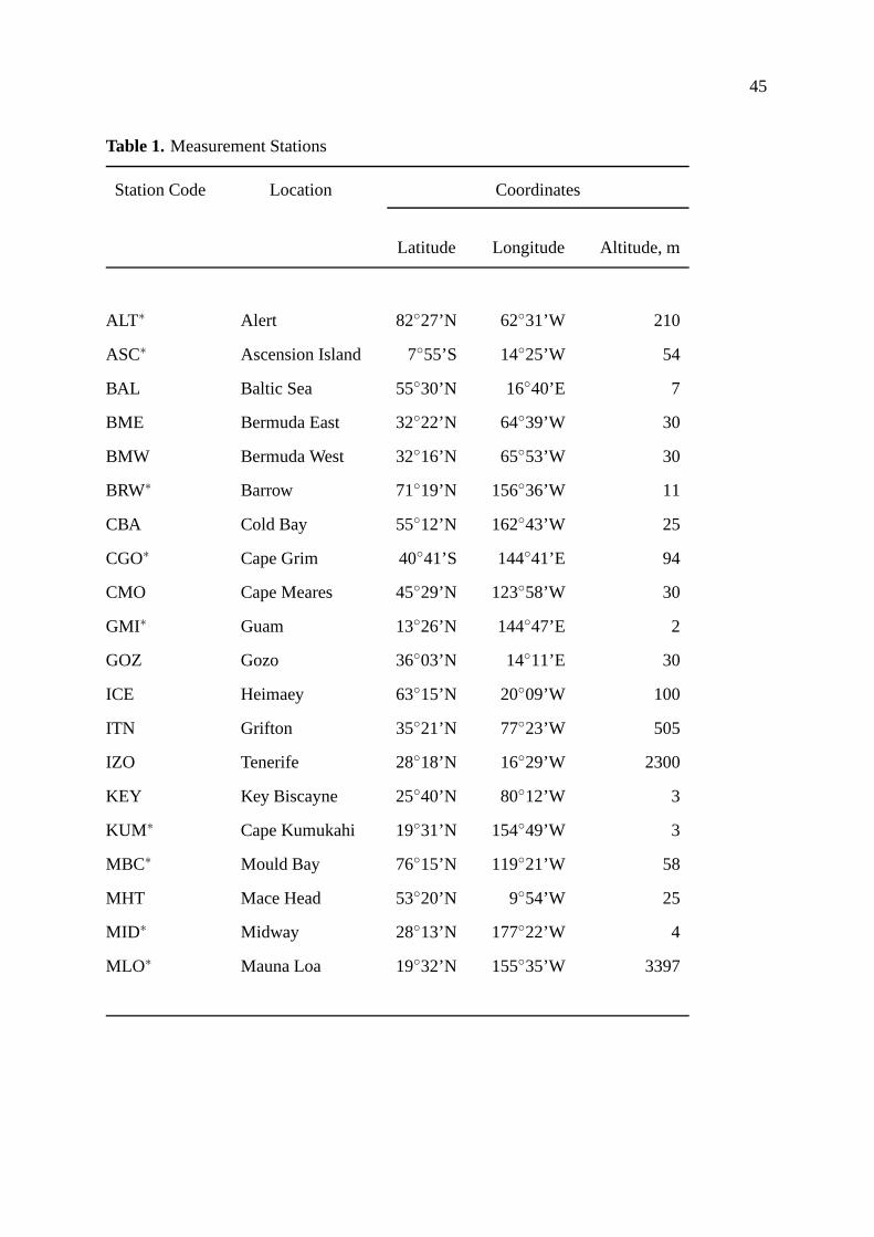
45
Table 1. Measurement Stations
Station Code Location Coordinates
Latitude Longitude Altitude, m
ALT∗ Alert 82◦27’N 62◦31’W 210
ASC∗ Ascension Island 7◦55’S 14◦25’W 54
BAL Baltic Sea 55◦30’N 16◦40’E 7
BME Bermuda East 32◦22’N 64◦39’W 30
BMW Bermuda West 32◦16’N 65◦53’W 30
BRW∗ Barrow 71◦19’N 156◦36’W 11
CBA Cold Bay 55◦12’N 162◦43’W 25
CGO∗ Cape Grim 40◦41’S 144◦41’E 94
CMO Cape Meares 45◦29’N 123◦58’W 30
GMI∗ Guam 13◦26’N 144◦47’E 2
GOZ Gozo 36◦03’N 14◦11’E 30
ICE Heimaey 63◦15’N 20◦09’W 100
ITN Grifton 35◦21’N 77◦23’W 505
IZO Tenerife 28◦18’N 16◦29’W 2300
KEY Key Biscayne 25◦40’N 80◦12’W 3
KUM∗ Cape Kumukahi 19◦31’N 154◦49’W 3
MBC∗ Mould Bay 76◦15’N 119◦21’W 58
MHT Mace Head 53◦20’N 9◦54’W 25
MID∗ Midway 28◦13’N 177◦22’W 4
MLO∗ Mauna Loa 19◦32’N 155◦35’W 3397

46
Table 1. (continued)
Station Code Location Coordinates
Latitude Longitude Altitude, m
NWR Niwot Ridge 40◦03’N 105◦35’W 3475
P01∗ Pacific cruise 10◦00’S 168◦36’W 0
P02∗ Pacific cruise 15◦00’S 175◦42’W 0
P03∗ Pacific cruise 25◦00’S 178◦00’E 0
P04∗ Pacific cruise 30◦00’S 177◦06’E 0
PSA∗ Palmer Station 64◦55’S 64◦00’W 10
QPC Qinghai Province 36◦16’N 100◦55’E 3810
RPB∗ Barbados 13◦10’N 59◦26’W 3
SC1 South China Sea cruise 3◦00’N 105◦12’E 0
SC2 South China Sea cruise 6◦00’N 107◦18’E 0
SC3 South China Sea cruise 9◦00’N 109◦24’E 0
SC4 South China Sea cruise 12◦00’N 111◦00’E 0
SC5 South China Sea cruise 15◦00’N 112◦18’E 0
SC6 South China Sea cruise 18◦00’N 113◦18’E 0
SC7 South China Sea cruise 21◦00’N 114◦00’E 0
SEY∗ Seychelles 4◦40’S 55◦10’E 3
SHM∗ Shemya Island 52◦43’N 174◦06’E 40
SMO∗ American Samoa 14◦15’S 170◦34’W 42

47
Table 1. (continued)
Station Code Location Coordinates
Latitude Longitude Altitude, m
SPO∗ South Pole 89◦59’S 24◦48’W 2810
STM∗ Ocean Station “M” 66◦00’N 2◦00’E 7
SYO∗ Syowa 69◦00’S 39◦35’E 11
TAP Tae-ahn Peninsula 36◦44’N 126◦08’E 20
UTA Utah 39◦54’N 113◦43’W 1320
UUM Ulaan Uul 44◦27’N 111◦06’E 914
ZEP Ny-Alesund 78◦54’N 11◦53’E 475
∗Station is used to derive the global mean trend.

48
Table 2. A Priori CH4 Fluxes and Uncertainties
Process Annual Total Uncertainty a Seasonality Reference b,c
Anthropogenic Surface Fluxes
Oil/gas production 51 ± 30 . . . OL(1,3)
Coal mining 38 ± 15 . . . OL(1,3)
Landfills 48 ± 20 . . . OL(1,3)
Domestic ruminants 93 ± 35 . . . OL(1,3)
Biomass burning 40 ± 30 part of the dry season LE(1), OL(3), H91(4)
Rice agriculture 80 ± 50 dependent on the LE(1), M91(3,4)
growing season
Other sources d 20 ± 16 . . . OL(1,3)
Natural Surface Fluxes
Tropical wetlands 91 ± 26 . . . LE(1), M87(3)
Boreal/arctic wetlands 54 ± 15 temperature dependent LE(1), M87(3), RH(4)
Termites 20 ± 20 . . . LE(1), SA(3)
Oceans 15 ± 10 . . . LE(1), PS(3)
Volcanoes 3.5 ± 3 . . . LA(1), PS(3)
Wild animals 5 ± 5 . . . LE(1), PS(3)
Soil oxidation -30 ± 15 . . . LE(1), FU(3)
Total 528 ± 90
Fluxes and uncertainties in Tg(CH4) yr−1.
aA 95% uncertainty interval (± 2σ) is used.

49
bReferences are 1 annual and global flux total; 2 uncertainty in 1 (Lelieveld et al. [1998] if not stated
explicitly); 3 spatial distribution; and 4 seasonality.
cReferences are OL, Olivier et al. [1996]; CR, Crutzen [1995]; LE, Lelieveld et al. [1998]; H91, Hao et al.
[1991]; M91, Matthews et al. [1991]; M87, Matthews and Fung [1987]; RH, Hein et al. [1997]; SA, Sanderson
[1996]; LA, Lacroix [1993]; FU, Fung et al. [1991]; and PS, present study (see text).
dOther sources are the sum of fossil fuel and domestic biofuel combustion, and industrial production of iron,
steel, and chemicals.

50
Table 3. Standard Scenario Integrated CH4 Fluxes and Uncertainties
A priori A posteriori
Mean Uncertainty a Mean Uncertainty a
Surface flux
Globe 528 ± 90 505 ± 24
Northern Hemisphere (NH) 405 ± 81 340 ± 19
Southern Hemisphere (SH) 123 ± 40 165 ± 18
Tropospheric OH 485 ± 25 451 ± 22
Stratospheric loss 40 ± 10 37 ± 9.7
Trend 3 ± 94 18 ± 7
c0 1.696 . . . b 1.694 ± 0.009
Fluxes and uncertainties are in Tg(CH4) yr−1.
aA 95% uncertainty interval (± 2σ) is used.
bInitial methane concentration is in ppmv (see (3)). Uncertainty in c0 is set to a high value.

51
Table 4. Uncertainty Reduction per Station
Global Local
Station Uncertainty Reduction,a% Station Uncertainty Reduction, %
1. SPO 83 QPC 45
2. SYO 81 TAP 39
3. P24 75 GMI 39
4. PSA 74 SC7 32
5. P25 71 SC5 20
6. P22 63 SC6 18
7. CGO 58 SEY 16
8. ASC 48 UUM 16
9. SMO 46 SC4 15
10. MLO 42 SC3 14
11. P20 37 GOZ 12
12. GMI 37 MHT 12
13. QPC 34 IZO 11
14. MID 34 STM 10
15. SHM 34 UTA 9...
...
41. TAP 13 CMO 2
42. UTA 13 P25 1
43. GOZ 13 P24 1
44. ITN 5 ALT <0.5

52
Table 4. (continued)
Global Local
Station Uncertainty Reduction,a% Station Uncertainty Reduction, %
45. BAL 4 SPO <0.5
aUncertainty reductions are relative to the uncertainty reductions in a standard inversion (see
text).

53
Table 5. Sensitivity Tests, Integrated CH4 Fluxes and Uncertainties
Globe NH SH Region 1 a Region 2 b
A PrioriAll inversions 528 (±90)c 405 (±81) 123 (±40) 111 (±56) 51 (±28)
A PosterioriStandard 505 (±24) 340 (±19) 165 (±18) 77 (±23) 65 (±20)
Time correlation 500 (±23) 338 (±17) 162 (±16) 80 (±20) 65 (±18)
Space correlation 481 (±22) 333 (±15) 148 (±13) 78 (±15) 63 (±14)
Relative uncertainty (600%) 511 (±25) 343 (±21) 169 (±20) 76 (±27) 68 (±25)
Relative uncertainty (100%) 479 (±15) 338 (±9) 142 (±8) 75 (±8) 54 (±6)
OH ratio (NH/SH=2) 516 (±24) 395 (±20) 121 (±17) 103 (±23) 69 (±20)
Fluxes and uncertainties in Tg(CH4) yr−1.
aRegion 1 is 75◦–135◦E, 10◦–40◦N (southeast Asia).
bRegion 2 is 5◦W–35◦E, 15◦S–25◦N (central Africa).
cA 95% uncertainty interval (± 2σ) is used. The a priori uncertainties correspond to
the standard scenario only.

54
Table 6. Standard and Low Rice Scenarios, Integrated CH4 Fluxes, and
Uncertainties
Scenario Globe NH SH Zone a Region b
A priori
Standard 528 (±90) 405 (±81) 123 (±40) 212 (±66) 111 (±56)
Low rice 528 (±77) 384 (±66) 143 (±38) 185 (±47) 74 (±31)
A posteriori
Standard 505 (±24) 340 (±19) 165 (±18) 169 (±25) 77 (±23)
Low rice 508 (±24) 342 (±18) 166 (±17) 164 (±23) 68 (±18)
Fluxes are in Tg(CH4) yr−1.
aThe zonal band is from 10◦–40◦N.
bThe region is 75◦–135◦W, 10◦–40◦N.
cA 95% uncertainty interval (± 2σ) is used.

55
FiguresMace Head(53N,10W)
1977.0 1978.6 1980.3 1981.9 1983.5 1985.2 1986.8 1988.5 1990.1 1991.7 1993.4 1995.0year
60
80
100
120
140
160
CH
3CC
l3 (
pptv
)
Oregon(45N,124W)
1977.0 1978.6 1980.3 1981.9 1983.5 1985.2 1986.8 1988.5 1990.1 1991.7 1993.4 1995.0year
60
80
100
120
140
160
CH
3CC
l3 (
pptv
)
Barbados(13N,59W)
1977.0 1978.6 1980.3 1981.9 1983.5 1985.2 1986.8 1988.5 1990.1 1991.7 1993.4 1995.0year
60
80
100
120
140
CH
3CC
l3 (
pptv
)
Samoa(14S,171W)
1977.0 1978.6 1980.3 1981.9 1983.5 1985.2 1986.8 1988.5 1990.1 1991.7 1993.4 1995.0year
40
60
80
100
120
CH
3CC
l3 (
pptv
)
Tasmania(41S,145E)
1977.0 1978.6 1980.3 1981.9 1983.5 1985.2 1986.8 1988.5 1990.1 1991.7 1993.4 1995.0year
40
60
80
100
120
CH
3CC
l3 (
pptv
)
Figure 1. Comparison of modeled 1,1,1-trichloroethane (CH3CCl3) concentrations to mea-
surements at the Atmospheric Lifetime Experiment (ALE)/ Global Atmospheric Gases Exper-
iment (GAGE) stations. Solid lines are optimized OH fields; dashed lines are original OH
fields; and squares are monthly mean measurements. Error bars represent the 1σ interval of the
measurements.

56
a
b
c
Figure 2. Estimated surface fluxes of methane for (left) January and (right) July: (a) a priori,
(b) a posteriori, and (c) difference a posteriori minus a priori.
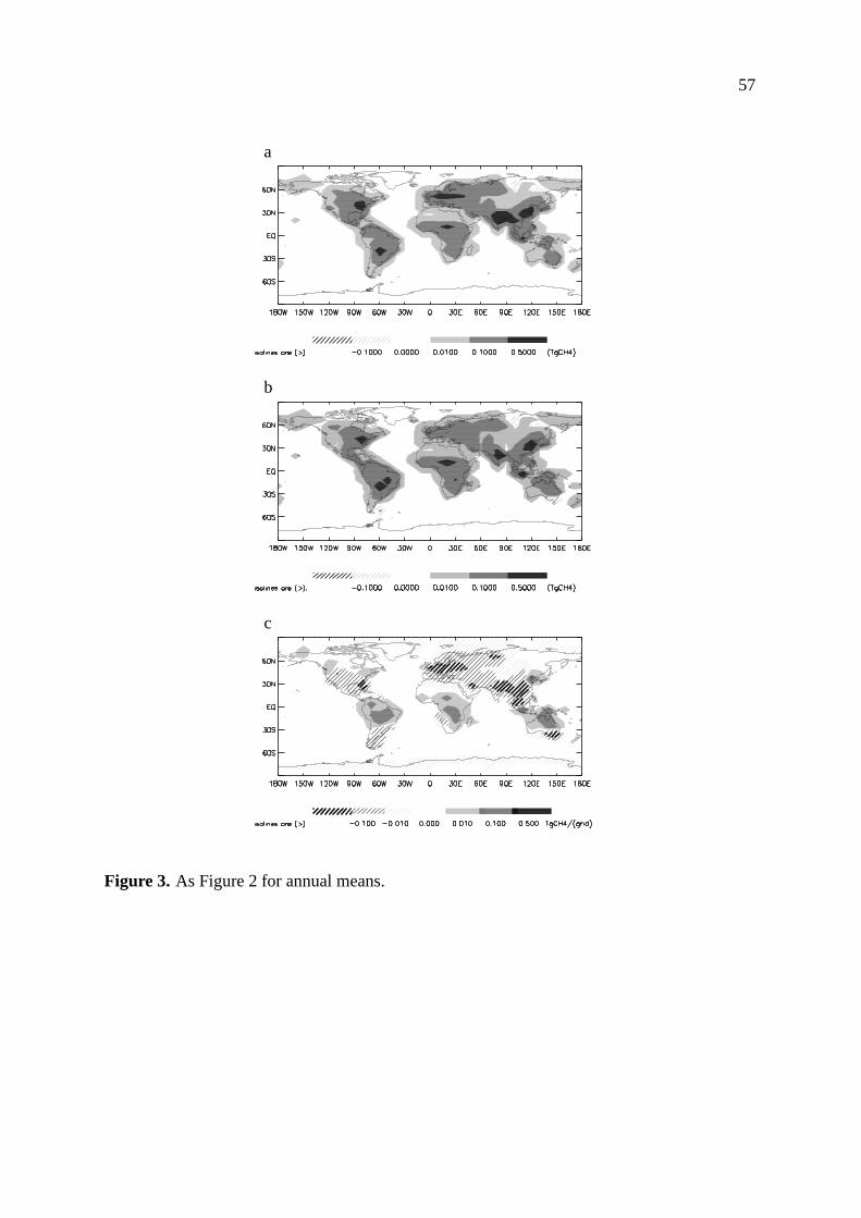
57
a
b
c
Figure 3. As Figure 2 for annual means.

58
ALT
J F M A M J J A S O N D
1.75
1.80
1.85
CH
4(pp
mv)
CMO
J F M A M J J A S O N D
1.72
1.74
1.76
1.78
1.80
1.82
1.84
CH
4(pp
mv)
KUM
J F M A M J J A S O N D
1.68
1.70
1.72
1.74
1.76
1.78
1.80
1.82
CH
4(pp
mv)
MID
J F M A M J J A S O N D 1.68
1.70
1.72
1.74
1.76
1.78
1.80
1.82
CH
4(pp
mv)
P24
J F M A M J J A S O N D
1.62
1.64
1.66
1.68
1.70
1.72
1.74
CH
4(pp
mv)
SPO
J F M A M J J A S O N D
1.62
1.64
1.66
1.68
1.70
1.72
CH
4(pp
mv)
Figure 4. Comparison of simulated concentrations to measurements. Dashed lines represent
simulations based on a priori fluxes; solid lines represent simulations based on a posteriori
fluxes; and squares represent monthly means of observations. Error bars represent the 1σ
interval of the measurements. The offset of the a priori data has been adjusted according to the
offset at the South Pole.

59
-90 -45 0 45 90Latitude (degrees)
1.65
1.70
1.75
1.80
1.85
1.90
CH
4(pp
mv)
Figure 5. Observed and simulated latitudinal methane concentration gradients (representing
annual means). Squares represent simulations based a priori fluxes; triangles represent simula-
tions based on a posteriori fluxes; and solid circles represent measurements. The offset in the a
priori data has been adjusted according to the offset at the South Pole.

60
a
b
c
Figure 6. Reduction in surface flux uncertainty gained by the inversion (1 −
σaposteriori/σapriori): (a) January, (b) July, (c) annual mean.

61
a
b
Figure 7. (a) A posteriori uncertainty covariances between the July flux for a grid in Brazil and
all remaining fluxes for July and (b) the same as Figure 7a but for a grid in China. Covariances
are expressed in units of the corresponding (Brazilian or Chinese) variances. (Consequently,
these Chinese and Brazilian grids both have a value of 1.)

62
CBA
J F M A M J J A S O N D
1.72
1.74
1.76
1.78
1.80
1.82
1.84
1.86
CH
4(pp
mv)
MHT
J F M A M J J A S O N D
1.74
1.76
1.78
1.80
1.82
1.84
CH
4(pp
mv)
ITN
J F M A M J J A S O N D
1.75
1.80
1.85
1.90
CH
4(pp
mv)
MLO
J F M A M J J A S O N D
1.68
1.70
1.72
1.74
1.76
1.78
1.80
CH
4(pp
mv)
GMI
J F M A M J J A S O N D
1.66
1.68
1.70
1.72
1.74
1.76
1.78
CH
4(pp
mv)
SC5
J F M A M J J A S O N D
1.70
1.75
1.80
CH
4(pp
mv)
ASC
J F M A M J J A S O N D
1.64
1.66
1.68
1.70
1.72
1.74
CH
4(pp
mv)
CGO
J F M A M J J A S O N D
1.62
1.64
1.66
1.68
1.70
1.72
CH
4(pp
mv)
SPO
J F M A M J J A S O N D
1.62
1.64
1.66
1.68
1.70
1.72
CH
4(pp
mv)
Figure 8. Comparison between simulated and observed concentrations. Measurements at these
locations have been excluded from the inversion. Dashed lines represent a priori; solid lines
represent a posteriori; and squares represent measurements. Error bars represent 1σ interval of
the measurements.

63
Figure 9. Seasonal cycles in the estimated fluxes for four regions. Solid lines are uncorrelated
fluxes; dashed lines are time-orrelated fluxes (see text); and dotted lines are a priori fluxes.
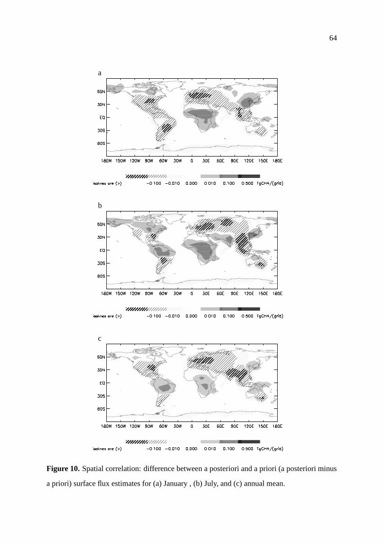
64
a
b
c
Figure 10. Spatial correlation: difference between a posteriori and a priori (a posteriori minus
a priori) surface flux estimates for (a) January , (b) July, and (c) annual mean.