Inverse and Direct Kinematics of Hexa Parallel Robot of ...Angie J Valencia C, Mauricio Mauledoux, and Diego A. Nunez Faculty of Engineering, Militar Nueva Granada University, Bogota,

748

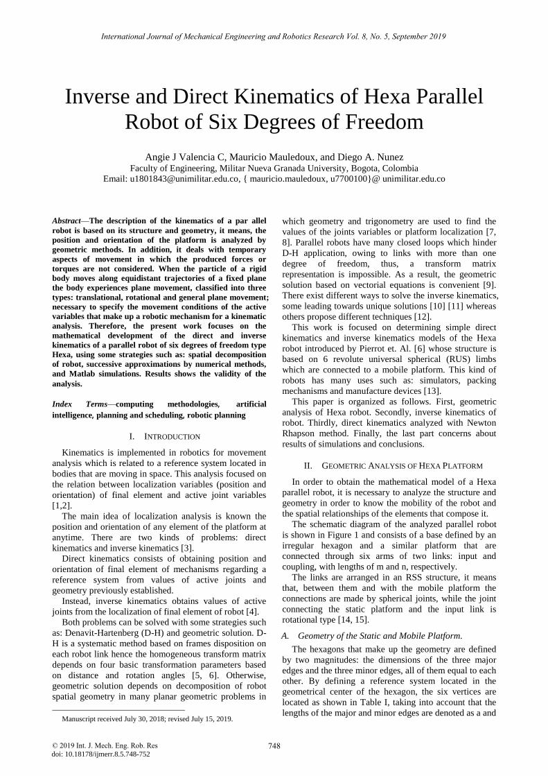
International Journal of Mechanical Engineering and Robotics Research Vol. 8, No. 5, September 2019

© 2019 Int. J. Mech. Eng. Rob. Resdoi: 10.18178/ijmerr.8.5.748-752

Inverse and Direct Kinematics of Hexa Parallel

Robot of Six Degrees of Freedom

Angie J Valencia C, Mauricio Mauledoux, and Diego A. Nunez Faculty of Engineering, Militar Nueva Granada University, Bogota, Colombia

Email: [email protected], { mauricio.mauledoux, u7700100}@ unimilitar.edu.co

Abstract—The description of the kinematics of a par allel

robot is based on its structure and geometry, it means, the

position and orientation of the platform is analyzed by

geometric methods. In addition, it deals with temporary

aspects of movement in which the produced forces or

torques are not considered. When the particle of a rigid

body moves along equidistant trajectories of a fixed plane

the body experiences plane movement, classified into three

types: translational, rotational and general plane movement;

necessary to specify the movement conditions of the active

variables that make up a robotic mechanism for a kinematic

analysis. Therefore, the present work focuses on the

mathematical development of the direct and inverse

kinematics of a parallel robot of six degrees of freedom type

Hexa, using some strategies such as: spatial decomposition

of robot, successive approximations by numerical methods,

and Matlab simulations. Results shows the validity of the

analysis.

Index Terms—computing methodologies, artificial

intelligence, planning and scheduling, robotic planning

I. INTRODUCTION

Kinematics is implemented in robotics for movement

analysis which is related to a reference system located in

bodies that are moving in space. This analysis focused on

the relation between localization variables (position and

orientation) of final element and active joint variables

[1,2].

The main idea of localization analysis is known the

position and orientation of any element of the platform at

anytime. There are two kinds of problems: direct

kinematics and inverse kinematics [3].

Direct kinematics consists of obtaining position and

orientation of final element of mechanisms regarding a

reference system from values of active joints and

geometry previously established.

Instead, inverse kinematics obtains values of active

joints from the localization of final element of robot [4].

Both problems can be solved with some strategies such

as: Denavit-Hartenberg (D-H) and geometric solution. D-

H is a systematic method based on frames disposition on

each robot link hence the homogeneous transform matrix

depends on four basic transformation parameters based

on distance and rotation angles [5, 6]. Otherwise,

geometric solution depends on decomposition of robot

spatial geometry in many planar geometric problems in

Manuscript received July 30, 2018; revised July 15, 2019.

which geometry and trigonometry are used to find the

values of the joints variables or platform localization [7,

8]. Parallel robots have many closed loops which hinder

D-H application, owing to links with more than one

degree of freedom, thus, a transform matrix

representation is impossible. As a result, the geometric

solution based on vectorial equations is convenient [9].

There exist different ways to solve the inverse kinematics,

some leading towards unique solutions [10] [11] whereas

others propose different techniques [12].

This work is focused on determining simple direct

kinematics and inverse kinematics models of the Hexa

robot introduced by Pierrot et. Al. [6] whose structure is

based on 6 revolute universal spherical (RUS) limbs

which are connected to a mobile platform. This kind of

robots has many uses such as: simulators, packing

mechanisms and manufacture devices [13].

This paper is organized as follows. First, geometric

analysis of Hexa robot. Secondly, inverse kinematics of

robot. Thirdly, direct kinematics analyzed with Newton

Rhapson method. Finally, the last part concerns about

results of simulations and conclusions.

II. GEOMETRIC ANALYSIS OF HEXA PLATFORM

In order to obtain the mathematical model of a Hexa

parallel robot, it is necessary to analyze the structure and

geometry in order to know the mobility of the robot and

the spatial relationships of the elements that compose it.

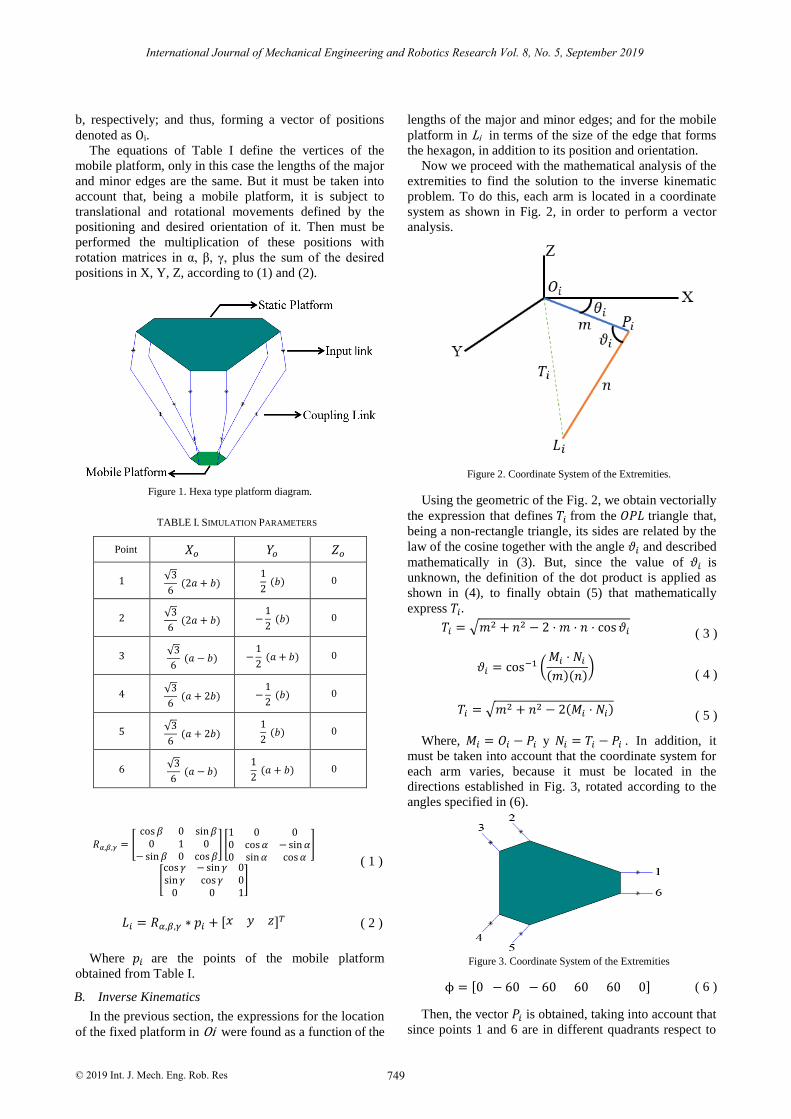
The schematic diagram of the analyzed parallel robot

is shown in Figure 1 and consists of a base defined by an

irregular hexagon and a similar platform that are

connected through six arms of two links: input and

coupling, with lengths of m and n, respectively.

The links are arranged in an RSS structure, it means

that, between them and with the mobile platform the

connections are made by spherical joints, while the joint

connecting the static platform and the input link is

rotational type [14, 15].

A. Geometry of the Static and Mobile Platform.

The hexagons that make up the geometry are defined

by two magnitudes: the dimensions of the three major

edges and the three minor edges, all of them equal to each

other. By defining a reference system located in the

geometrical center of the hexagon, the six vertices are

located as shown in Table I, taking into account that the

lengths of the major and minor edges are denoted as a and

749


© 2019 Int. J. Mech. Eng. Rob. Res

b, respectively; and thus, forming a vector of positions

denoted as Oi.

The equations of Table I define the vertices of the

mobile platform, only in this case the lengths of the major

and minor edges are the same. But it must be taken into

account that, being a mobile platform, it is subject to

translational and rotational movements defined by the

positioning and desired orientation of it. Then must be

performed the multiplication of these positions with

rotation matrices in α, β, γ, plus the sum of the desired

positions in X, Y, Z, according to (1) and (2).

Figure 1.

Hexa type platform diagram.

TABLE I. SIMULATION PARAMETERS

Point 𝑋𝑜 𝑌𝑜 𝑍𝑜

1 √3

6 (2𝑎 + 𝑏)

1

2 (𝑏) 0

2 √3

6 (2𝑎 + 𝑏) −

1

2 (𝑏) 0

3 √3

6 (𝑎 − 𝑏) −

1

2 (𝑎 + 𝑏) 0

4 √3

6 (𝑎 + 2𝑏) −

1

2 (𝑏) 0

5 √3

6 (𝑎 + 2𝑏)

1

2 (𝑏) 0

6 √3

6 (𝑎 − 𝑏)

1

2 (𝑎 + 𝑏) 0

𝑅𝛼,𝛽,𝛾 = [cos 𝛽 0 sin 𝛽

0 1 0− sin 𝛽 0 cos 𝛽

] [1 0 00 cos 𝛼 − sin 𝛼0 sin 𝛼 cos 𝛼

]

[cos 𝛾 − sin 𝛾 0sin 𝛾 cos 𝛾 0

0 0 1]

( 1 )

𝐿𝑖 = 𝑅𝛼,𝛽,𝛾 ∗ 𝑝𝑖 + [𝑥 𝑦 𝑧]𝑇 ( 2 )

Where 𝑝𝑖 are the points of the mobile platform

obtained from Table I.

B. Inverse Kinematics

In the previous section, the expressions for the location

of the fixed platform in Oi were found as a function of the

lengths of the major and minor edges; and for the mobile

platform in Li in terms of the size of the edge that forms

the hexagon, in addition to its position and orientation.

Now we proceed with the mathematical analysis of the

extremities to find the solution to the inverse kinematic

problem. To do this, each arm is located in a coordinate

system as shown in Fig. 2, in order to perform a vector

analysis.

Figure 2. Coordinate System of the Extremities.

Using the geometric of the Fig. 2, we obtain vectorially

the expression that defines 𝑇𝑖 from the 𝑂𝑃𝐿 triangle that,

being a non-rectangle triangle, its sides are related by the

law of the cosine together with the angle 𝜗𝑖 and described

mathematically in (3). But, since the value of 𝜗𝑖 is

unknown, the definition of the dot product is applied as

shown in (4), to finally obtain (5) that mathematically

express 𝑇𝑖 .

𝑇𝑖 = √𝑚2 + 𝑛2 − 2 ⋅ 𝑚 ⋅ 𝑛 ⋅ cos 𝜗𝑖

( 3 )

𝜗𝑖 = cos−1 (𝑀𝑖 ⋅ 𝑁𝑖

(𝑚)(𝑛))

( 4 )

𝑇𝑖 = √𝑚2 + 𝑛2 − 2(𝑀𝑖 ⋅ 𝑁𝑖)

( 5 )

Where, 𝑀𝑖 = 𝑂𝑖 − 𝑃𝑖 y 𝑁𝑖 = 𝑇𝑖 − 𝑃𝑖 . In addition, it

must be taken into account that the coordinate system for

each arm varies, because it must be located in the

directions established in Fig. 3, rotated according to the

angles specified in (6).

Figure 3. Coordinate System of the Extremities

ϕ = [0 − 60 − 60 60 60 0] ( 6 )

Then, the vector 𝑃𝑖 is obtained, taking into account that

since points 1 and 6 are in different quadrants respect to

750



points 2 to 5, two different equations must be considered.

For 1 and 6 the value of 𝑃𝑖 is described in (7) and for the

others in (8).

For the magnitude of 𝑇𝑖 , the mathematics are defined

by the Pythagorean theorem as shown in (9).

𝑇𝑖 = √(𝑋𝐿𝑖− 𝑋𝑜)

2+ (𝑌𝐿𝑖

− 𝑦𝑜)2

+ (𝑍𝐿𝑖)

2

( 9 )

Taking in to account the two equations for 𝑇𝑖 in (5) and

(9), the terms are equated to find the equation of each arm,

adopting the form of (10), according to Fig. 4. Where 𝐴𝑖,

𝐵𝑖 and 𝐶𝑖, vary depending of the working point, so (11)

are defined for points 1 and 6 and (12) for points 2 to 5.

Figure 4. Graphical representation of (10).

𝐴𝑖 sin 𝜃𝑖 + 𝐵𝑖 cos 𝜃𝑖 = 𝐶𝑖 ( 10 )

𝐴𝑖 = 2 ⋅ 𝑚 ⋅ (𝑍𝐿𝑖− 𝑍𝑜)

𝐵𝑖 = 2 ⋅ 𝑚 ⋅ (𝑐𝑜𝑠(𝜙𝑖) ⋅ (𝑋𝑜 − 𝑋𝐿𝑖) + 𝑠𝑖𝑛(𝜙𝑖) ⋅ (𝑌𝐿𝑖

− 𝑌𝑜))

𝐶𝑖 = 𝑛2 − 𝑚2 − (𝑋𝑜 − 𝑋𝐿𝑖)

2− (𝑌𝑜 − 𝑌𝐿𝑖

)2

− (𝑍𝑜 − 𝑍𝐿𝑖)

2

( 11 )

𝐴𝑖 = 2 ⋅ 𝑚 ⋅ (𝑍𝐿𝑖− 𝑍𝑜)

𝐵𝑖 = 2 ⋅ 𝑚 ⋅ (𝑐𝑜𝑠(𝜙𝑖) ⋅ (𝑋𝐿𝑖− 𝑋𝑜) + 𝑠𝑖𝑛(𝜙𝑖) ⋅ (𝑌𝐿𝑖

− 𝑌𝑜))

𝐶𝑖 = 𝑛2 − 𝑚2 − (𝑋𝑜 − 𝑋𝐿𝑖)

2− (𝑌𝑜 − 𝑌𝐿𝑖

)2

− (𝑍𝑜 − 𝑍𝐿𝑖)

2

( 12 )

To finally obtain the value of the angle 𝜃𝑖 of each arm,

implementing (13).

𝜃𝑖 = cos−1 (𝐶𝑖

√𝐴𝑖2 + 𝐵𝑖

2) + tan−1 (

𝐴𝑖

𝐵𝑖

) ( 13 )

C. Direct Kinematics

Direct kinematics is solved base on (14), which

determines the length of link in terms of tridimensional

positions of points 𝑃𝑖 y 𝐿𝑖.

𝑛2 = (𝑋𝐿𝑖− 𝑋𝑃𝑖

)2

+ (𝑌𝐿𝑖− 𝑌𝑃𝑖

)2

+ (𝑍𝐿𝑖− 𝑍𝑃𝑖

)2 ( 14 )

Applying (14) for each arm of robot, a no-lineal

equation system was determined due to 𝑋𝐿𝑖, 𝑌𝐿𝑖

y 𝑍𝐿𝑖 are

expresed in position and orientation terms of mobil

platform. Hence, there are six unknowns 𝑥, 𝑦, 𝑧, 𝛼, 𝛽, 𝛾

which are express in 6x6 equation system showed in (15).

𝑓𝑖 = (𝑋𝐿𝑖− 𝑋𝑃𝑖

)2

+ (𝑌𝐿𝑖− 𝑌𝑃𝑖

)2

+ (𝑍𝐿𝑖− 𝑍𝑃𝑖

)2

− 𝑛2 = 0 ( 15 )

Previous system has a unique solution and it can be

resolved with numeric methods, for instance, Newton

Raphson multivariable method. That method requires

Jacobian Matrix [13] which is expressed in (16).

𝑓´𝑥𝑖 =𝜕𝑓𝑖

𝜕𝑥, 𝑓´𝑦𝑖 =

𝜕𝑓𝑖

𝜕𝑦, 𝑓´𝑧𝑖 =

𝜕𝑓𝑖

𝜕𝑧

𝑓´𝛼𝑖 =𝜕𝑓𝑖

𝜕𝛼, 𝑓´𝛽𝑖 =

𝜕𝑓𝑖

𝜕𝛽, 𝑓´𝛾𝑖 =

𝜕𝑓𝑖

𝜕𝛾

(16 )

Newton Rhapson method is implemented based on

(17), objective function is related to (18).

[𝑥, 𝑦, 𝑧, 𝛼, 𝛽, 𝛾]𝑖+1 = [𝑥, 𝑦, 𝑧, 𝛼, 𝛽, 𝛾] −𝑓𝑖

𝑓´𝑖

( 17 )

𝑒𝑟𝑟𝑜𝑟 = ((𝑋 − 𝑋𝑑)2 + (𝑌 − 𝑌𝑑)2 + (𝑍 − 𝑍𝑑)2

+ (𝛼 − 𝛼𝑑)2 + (𝛽 − 𝛽𝑑)2

+ (𝛾 − 𝛾𝑑)2)1/2 ≤ 𝑡𝑜𝑙 ( 18 )

If the determinant of Jacobian matrix is equal zero, the

matrix will be singular, and its inverse cannot be

calculated. This case describes that robot loses mobility

or cannot reach the required position because of its

geometry. Therefore, its important calculate the inverse

matrix following (19) [16, 17].

𝑑𝑞

𝑑𝑡= 𝑓′(𝑞) ⋅ �̇� ( 19 )

Where 𝑞 denoted generalized coordinates: 𝑥 , 𝑦 , 𝑧 , 𝛼 ,

𝛽, 𝛾.

III. RESULTS AND DISCUSSIONS

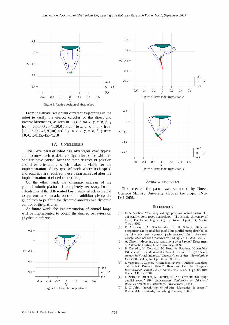
The simulation of the previously established

calculations is performed with the values specified in

Table II. And we start from a resting position for 𝑥, 𝑦, 𝑧,

in meters 𝛼, 𝛽 , 𝛾 in degrees of [ 0, 0, −0.45, 0, 0, 0] of

the robot as shown in Fig. 5.

TABLE II: SIMULATION PARAMETERS

Parameter Value

𝑚 0.15 𝑚

𝑛 0.35 𝑚

𝑎 0.3 𝑚

𝑏 0.1 𝑚

𝑐 0.05 𝑚

𝑃𝑖 = [

𝑚 ⋅ 𝑐𝑜𝑠(𝜃𝑖) ⋅ 𝑐𝑜𝑠(𝜙𝑖) + 𝑋𝑜

−𝑚 ⋅ 𝑐𝑜𝑠(𝜃𝑖) ⋅ 𝑠𝑖𝑛(𝜙𝑖) + 𝑌𝑜

−𝑚 ⋅ 𝑠𝑖𝑛(𝜃𝑖) + 𝑍𝑜];]

( 7 )

𝑃𝑖 = [

−𝑚 ⋅ 𝑐𝑜𝑠(𝜃𝑖) ⋅ 𝑐𝑜𝑠(𝜙𝑖) + 𝑋𝑜

−𝑚 ⋅ 𝑐𝑜𝑠(𝜃𝑖) ⋅ 𝑠𝑖𝑛(𝜙𝑖) + 𝑌𝑜

−𝑚 ⋅ 𝑠𝑖𝑛(𝜃𝑖) + 𝑍𝑜];]

( 8 )

751



Figure 5. Resting position of Hexa robot

From the above, we obtain different trajectories of the

robot to verify the correct calculus of the direct and

inverse kinematics, as seen in Figs. 6 for x, y, z, α, β, γ

from [ 0,0.5,-0.25,45,20,0], Fig. 7 to x, y, z, α, β, γ from

[ 0,-0.5,-0.2,45,20,30] and Fig. 8 to x, y, z, α, β, γ from

[ 0,-0.1,-0.35,-45,-45,10].

IV. CONCLUSIONS

The Hexa parallel robot has advantages over typical

architectures such as delta configuration, since with this

one can have control over the three degrees of position

and three orientation, which makes it viable for the

implementation of any type of work where both speed

and accuracy are required, these being achieved after the

implementation of closed control loops.

On the other hand, the kinematic analysis of the

parallel robotic platform is completely necessary for the

calculation of the differential kinematics, which is crucial

to perform a kinematic control, in addition giving the

guidelines to perform the dynamic analysis and dynamic

control of the platform.

As future work, the implementation of control loops

will be implemented to obtain the desired behaviors on

physical platforms.

Figure 6. Hexa robot in position 1



ACKNOWLEDGEMENT

The research for paper was supported by Nueva

Granada Military University, through the project ING-

IMP-2658.

REFERENCES

[1] H. A. Alashqat, “Modeling and high precision motion control of 3 dof parallel delta robot manipulator,” The Islamic University of

Gaza, Faculty of Engineering, Electrical Department, Master

Thesis, 2013.

[2] E. Mirshekari, A. Ghanbarzabeh, K. H. Shirazi, “Structure

comparison and optimal design of 6-rus parallel manipulator based on kinematic and dynamic performances,” Latin American

Journal of Solids and Structures, vol. 13, pp. 2414 – 2438, 2016.

[3] A. Olsson, “Modelling and control of a delta 3 robot” Department of Automatic Control, Lund University, 2009.

[4] P. Zamudio, V. Gonzalez, M. Parra, A. Ramirez, “Cinemática

Diferencial de un Manipulador Paralelo Plano 3RRR-(RRR) con Actuación Virtual Indirecta,” Ingeniería mecánica – Tecnologia y

Desarrollo, vol. 6, no. 3, pp 321 – 331, 2016.

[5] J. Vázquez, F. Cuenca, “Cinemática Inversa y Análisis Jacobiano del Robot Paralelo Hexa,” Memorias Del Xv Congreso

Internacional Annual De La Somim, vol. 1, no. 4, pp 800-810,

Sonora. México, 2009. [6] F. Pierrot, P. Dauchez, A. Fournier, “HEXA: a fast six-DOF fully-

parallel robot,” Fifth International Conference on Advanced

Robotics ‘Robots in Unstructured Environments, 1991.

[7] J. C. John, “Introduction to robotics: Mechanics & control,”

Boston, Addison-Wesley Publishing Company, 1986.

752



[8] J. Sabater, “Control de Robots”. División de Ingeniería de Sistemas y Automática del Grupo de Tecnología Industrial de la

Universidad Miguel Hernández (UMH) Campus Elche, 2004.

[9] R. Cisneros, “Modelo Matemático de un Robot Paralelo de Seis Grados de Libertad,” National Institute of Advanced Industrial

Science and Technology, Santa Catarina Mártir, Cholula, Puebla,

2006. [10] C. Vaida, D. Pisla, F. Covaciu, B. Gherman, A. Pisla, and N.

Plitea, “Development of a control system for a HEXA parallel

robot,” IEEE International Conference on Automation, Quality and Testing, Robotics (AQTR), pp. 1-6, 2016.

[11] B. Mohammed, “Planning a trajectory of a 6-DOF parallel robot

HEXA,” Electrical and Information Technologies (ICEIT) International Conference, pp. 300-305, 2016.

[12] A. Zubizarreta, M. Larrea, E. Irigoyen, I. Cabanes, “Real time

parallel robot direct kinematic problem computation using neural networks,” in Proc. 10th International Conference on Soft

Computing Models in Industrial and Environmental Applications,

Advances in Intelligent Systems and Computing, vol. 368, pp. 285-295, 2015.

[13] S. Tartari, E. Lustosa, “Kinematics and workspace analysis of a

parallel architecture robot: The Hexa,” ABCM Symposium Series in Mechatronics, vol. 2, pp 158-165, 2006.

[14] R. C. Hibbeler, “Mecánica vectorial para ingenieros: Dinámica,”

Décima edición. México, Pearson Educación, 2004. [15] T. Yukio, F. Hiroaki, K. Masafumi, H. Kazuya, “6-RSS type

spatial in-parallel actuated mechanism with six degrees of

freedom,” Department of Mechanical Engineering and Science: Tokio Institute of Technology, 1998.

[16] W. S. Mark and M. Vidyasagar, Robot Dynamics and Control,

New York, John Wiley & Sons, 1989. [17] L. W. Tsai, Robot Analysis: The Mechanics of Serial and Parallel

Manipulators, Maryland, John Wiley & Sons, Inc., 1999.

Angie J Valencia C received the B.S degree in mechatronics engineering from Nueva

Granada Military University, Colombia, in

2015 and her MSc in mechatronics engineering from the same University in 2018.

Since 2015, she has joined the DaVinci Group

at the Nueva Granada Military University, Colombia, as researching assistant. Her

current research interests include Control

System, Modelling Systems, Quadrotor prototype, Optimization Technics and Robotics Platforms.

Mauricio Mauledoux received the B.S. in mechatronics engineering from Militar Nueva

Granada University, in 2005. In 2011 He

received the PhD degree in Mathematical models, numerical methods and software

systems (Red Diploma) from St. Petersburg

State Polytechnic University, Russia. In 2012, he joined the Department of Mechatronic

Engineering, at Militar Nueva Granada

University, in Colombia as Assistant Professor. His current research interests include Robotics, automatic

control, Multi-agent Systems, Smart Grids, and Optimization.

Diego A Nunez received the B.S. in

mechatronics engineering from Militar Nueva

Granada University in 2005 and the M.Sc in mechanical engineering from Andes

University in 2014. Currently, he is working

toward the Ph.D. degree in Applied Science at Militar Nueva Granada University. His

research interests include parallel robots,

optimization and additive manufacturing.

Documents

Inverse and Direct Kinematics of Hexa Parallel Robot of ...Angie J Valencia C, Mauricio Mauledoux, and Diego A. Nunez Faculty of Engineering, Militar Nueva Granada University, Bogota,