Embed Size (px)
Citation preview
Corvinus University Budapest Faculty of Business Administration
Inventory Models in Reverse Logistics
PhD Dissertation
by
Dobos Imre
November, 2006.
2
Contents
Preface 3
1. Reverse Logistics: A Framework 4
2. Economic Order Quantity Models in Reverse Logistics 17
2.1. A Reverse Logistics Model with Procurement and Repair 20
2.2. A Model with Procurement and Finite Repair Rate:
The Substitution Policy 33
2.3. A Model with Procurement and Finite Repair Rate:
The Continuous Supplement Policy 46
3. Inventory Models with Waste Disposal 55
3.1. A Repair Model with Three Stocking Point 57
3.2. A Recoverable Item Inventory System 68
3.3. A Production-Recycling Model with Buybacking 83
4. Production Planning in Reverse Logistics 100
5. Summary and Further Research 119
References 123
Appendix 129
3
Preface
Environmental conscious material and inventory management will be studied in this
dissertation. It is named as reverse, inverse, or waste disposal logistics in the last decade. In
the Hungarian literature there are no uniform definitions for this scientific area. This research
field is defined in English speaking countries as reverse logistics. A former name of this idea
was inverse logistics, but this name is used mainly in Japan.
The dissertation consists of three chapters. In the first chapter I define reverse logistics and its
problems.
In the second chapter I present six deterministic reverse logistics inventory models. These
inventory models were constructed in the last three decades. A natural extension of EOQ-type
inventory models was examined in the last decade. The first reverse logistic inventory model
was built in 1967. The second model was published in 1979. In the eighties no paper was
published on this research area. The European Union has aided some research projects in the
nineties to support European environmental regulation. The publication of new reverse
logistic inventory models is in progress nowadays. Main point of the research is now
inventory models with shortage. The dissertation contains all available deterministic EOQ-
type models without shortage.
The last chapter investigates shortly the influence of reverse logistics on production planning,
and on material requirements planning systems. EOQ-type reverse logistics models can be
used, as a basis for the dynamic lot size reverse logistic model. The first publication appeared
on this field in 2000. The solution of Wagner-Whitin-type reverse logistic model is not easy,
because of the complexity of dynamic programming algorithms. EOQ-type reverse logistic
models can serve as heuristics to solve such kind of inventory models. This is a potential
application of this research field.
And last I summarize the results of this dissertation.
4
1. Reverse Logistics: A Framework
1.1. Introduction
Collection of used products, as paper, bottle, and battery, is a known idea in modern
economies. Reuse, remanufacturing and recycling of cars and electronic appliances, and
disposal of hazardous waste are very recent research field. The listed activities include a very
broad area, and it seems to have different management problems. This chapter summarizes the
reverse logistics which offers a theoretical background to solve such kind of business
problems.
The reuse is not a new phenomenon in the practice, but a lot of publications are appeared in
the international literature in eighties, named reverse logistics. In Hungarian literature there
are only a few publications on this research field. The first publication is paper of Rixer
(1995). He has called this field as “inverse logistics”. Cselényi et al. (1997) has used the
expression “recycling logistics”, and Mike (2002) has given the name “reverse logistics”
which is used in English speaking countries. There are some new publications about reverse
logistics in Hungarian, as well. (Richter and Dobos (2003)), Dobos (2004)) Reverse logistics
includes not only the material flow from supplier to consumer, but also the material flow of
used products from consumer to producer and supplier, in order to reduce the burden of
environment.
The aim of this chapter is to present the international (mainly Anglo-Saxon) literature on this
field. The environmental regulation becomes rigorous in the European Union and in Hungary.
There are recently a lot of environmental regulations about wastes along the life cycle of a
product in the European Union. (For example, about used cars.)
The European Union plans to solve environmental problems in the near future by the help of
legal regulation. These include the use of renewable environmental resources and energy;
avoid wastes, and substitution of non-renewable resources.
The Hungarian Parliament has legislated a law about the waste management in 2000. The aim
of this law is to protect the human health and environment, to support the rational use of
5
resources, and to reduce the environmental load, in order to promote sustainable development
and economic growth. The law disposes of wastes and activities of its handling. This law does
not touch the emissions in the air, and nuclear hazardous wastes. Some of principles are
mentioned in this law, as prevention, responsibility of producer, divided responsibility,
pollutant pays principle, best available technique, cost efficiency, and so on. The law disposes
of responsibility of producers, retailers, consumers, and owners of wastes. Steps of waste
management and reuse, and explanation of ideas are included in the law. There are defined
collection and transportation of wastes, reuse of wastes and handling. Separate sections
present responsibility of handling of communal and hazardous wastes, and organization of
waste management. It is to emphasize obligation of publicity and information.
Firms must keep this law, but application of reverse logistic methods can lead to cost savings
in long range. Legal registration can not force enterprise to produce an environmental
conscious way, but economic earnings can result an environmental friendly production
structure of firms.
In this chapter I present shortly the development of reverse logistics, and then I show a
conceptual framework, considering the development of this idea in the last decades. After that
I look for answer the main questions of reverse logistics: “why-how-what-who”. And last I
analyze the participants of reverse logistics, examined the main management problems.
1.2. About development…
There were economic and historic causes of development of logistics, as it is for the reverse
logistics. Retailers have recognized the chance of takeback of products in the United States at
the end of eighties, as a tool of market growth. Control of takeback was not directed, because
there was no uniform and serious regulation of forms of return policies of used products. The
result of this development was that consumers have taken back a number of products. The
costs of this process have dramatically increased at the producers and at the retailers, which
has reduced the profitability and competitiveness of firms. They have recognized that an
effective reverse logistics system is an important integral part of corporate strategy of firms.
The importance of reverse logistics is out of question, but the application of this concept
makes more difficult that authors define reverse logistics differently, and the solution of
6
reverse logistics concepts differs from each other at firm level. Because of this difficult
applicability, I try to define the idea, and I determine the potential research fields of reverse
logistics.
1.2.1. Determination of the concept
The reverse logistics was first defined in the eighties. In this time there were published only a
few articles in the literature, so the theoretical basis of investigations was unsettled. One of
the first publications on this field is the paper of Lambert and Stock (1981). They have
defined reverse logistics, as a reverse material flow opposite to supply chain, which is a “bad”
process along the material flow of firms. It means that until material flow of traditional supply
chain occurs in supplier-producer-wholesaler-retailer-consumer chain, reverse logistics seizes
the return material flow of used products, in order to follow this process backward from
consumer to supplier.
After the negative definition of Lambert and Stock, Murphy and Poist (1989) have offered a
new approach to determine reverse logistics. They have defined reverse logistics, as a material
flow of products from consumers to producers in the supply chain. This definition is accepted
by Pohlen and Farris (1992), who prefer to apply marketing concepts to reverse logistics. The
importance of their paper is that they have named the final consumer, and they have
emphasized that the process is reverse in the supply chain. A drawback of this definition is
that they have not determined the main activities of reverse logistics, which makes more
difficult to limit the framework of reverse logistics.
In the nineties Stock (1992) has given a wide definition, which is a basis for waste
management. He stresses the role of logistics, which contains recycling, waste disposal,
substitution of hazardous material, reduction of resources, and reuse. This definition of Stock
is more accurate than that of earlier. The connection with supply chain activities is missing in
this general definition, and the reverse process is not emphasized, as well.
These last approaches are summarized by Kopicky et al. (1993). This definition contains all
above-mentioned activities, the reverse movement of materials along the supply chain,
opposite to traditional logistics. Kopicky et al. (1993) have introduced information flow in the
7
definition of reverse logistics, which helps on effective practical functioning of reverse
logistic systems.
Carter and Ellram (1998) have collected a number of definitions of reverse logistics. I will
cite one of the definitions. The more general definition is: “Reverse logistics is such an
activity, which helps to continue an environmental effective policy of firms with reuse of
necessary materials, remanufacturing, and with reduction of amount of necessary materials”.
This efficiency touches the personal in production, supply, and consumption process. Carter
and Ellram (1998) approach reverse logistics from point of view of environmental protection.
Environmental consciousness occurs at three level of activity of firms: governmental
regulation, social pressure, and voluntary self restriction.
A next definition contains both traditional and reverse logistics. Council of Logistics
Management defines logistics: Logistics is a successful, cost-effective planning, realization,
and control of raw material, work-in progress, final products, and connected information from
the beginning to consumption, in order to perform consumer’s needs.
Rogers and Tibben-Lembke (1999) defines reverse logistics, as: Logistics is a successful,
cost-effective planning, realization, and control of raw material, work-in progress, final
products, and connected information from consumption to the beginning, in interest of value
regain, and handling of wastes.
Reverse Logistics Executive Council (RLEC) has given a more general definition of reverse
logistics, which summarizes the above definitions: Reverse logistics is a movement of
materials from a typical final consumption in an opposite direction, in order to regain value,
or to dispose of wastes. This reverse activity includes tackback of damaged products, renewal
and enlargement of inventories through product takeback, remanufacturing of packaging
materials, reuse of containers, repair and renovation of products, and handling of obsolete
appliances.
European Working Group on Reverse Logistics (REVLOG) has given a similar definition of
reverse logistics in 1998. The difference is that the beginning of collection is not only the
consumption, but it can be also production, distribution, or use.
8
The development of concept of reverse logistics was presented. The concept has changed
dramatically in the last two decades. Till the first approach has considered reverse logistics, as
a bad direction, nowadays the theory of reverse logistics contains marketing, financial, and
environmental points of view. In nineteen’s reverse logistics has become a well established
theory. This complex definition supports the idea that reverse logistics covers all activities
along the supply chain.
1.3. Factors of reverse logistics: Why? – How? – What? – Who?
After definition of reverse logistics I examine the factors that stand behind this concept. Four
questions arise in this context: why, how, what, and who. These questions are answered by
Brito and Dekker (2002) most comprehensively.
1.3.1. Why?
This question contains two research fields. First, why send persons used products back, and
why accept others used items? I have mentioned the causes of reverse logistics in the second
section of these chapter, i.e. economic, legislative, and social consequences. These causes
touch the “receiver” of groups. Brito and Dekker (2002) distinguish direct and indirect gains
inside of economic advantages. Direct gains are the possibility of profit increase that means a
reduction of use of raw materials, decrease of costs of waste disposal, and value added
through reuse. Indirect advantages are the “green” image of a firm which is a factor of
competitiveness for enterprises. Experiences have supported that environmental conscious
functioning of firms results in a stable consumer connection. It is a competitive advantage of
firms that increases in profit chances. A strict legislative regulation is a new argument for
practical application of reverse logistic processes, which serves as a method for environmental
protection. The United States and the European Union are leading in environmental
legislation, which forces the firms to keep the law. Thirdly, voluntary social responsibility of
firms directs organizations to protect environment. In the practice this voluntary activity
increases in competitive advantages of firms.
A second area is to investigate the group of “sender”. They have decided to send back a used
product to the manufacturer. As by the “receiver”, three fields are to be analyzed: return by
manufacturers, distributors, and users.
9
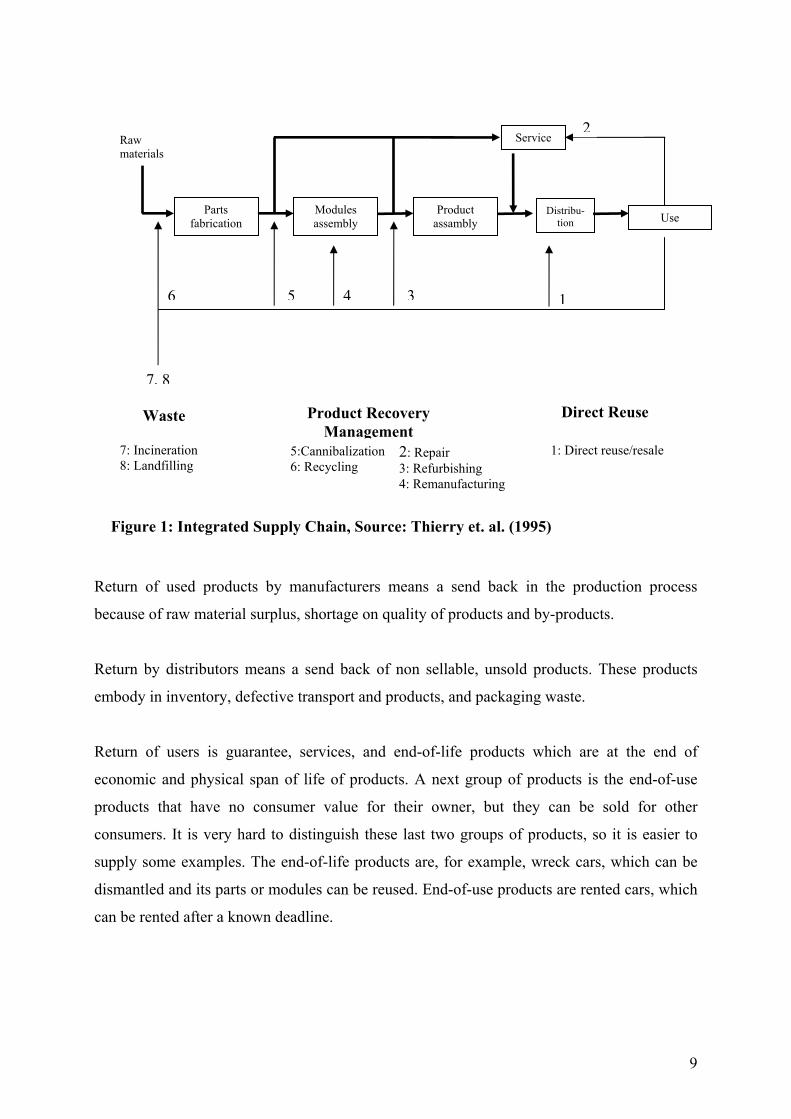
Return of used products by manufacturers means a send back in the production process
because of raw material surplus, shortage on quality of products and by-products.
Return by distributors means a send back of non sellable, unsold products. These products
embody in inventory, defective transport and products, and packaging waste.
Return of users is guarantee, services, and end-of-life products which are at the end of
economic and physical span of life of products. A next group of products is the end-of-use
products that have no consumer value for their owner, but they can be sold for other
consumers. It is very hard to distinguish these last two groups of products, so it is easier to
supply some examples. The end-of-life products are, for example, wreck cars, which can be
dismantled and its parts or modules can be reused. End-of-use products are rented cars, which
can be rented after a known deadline.
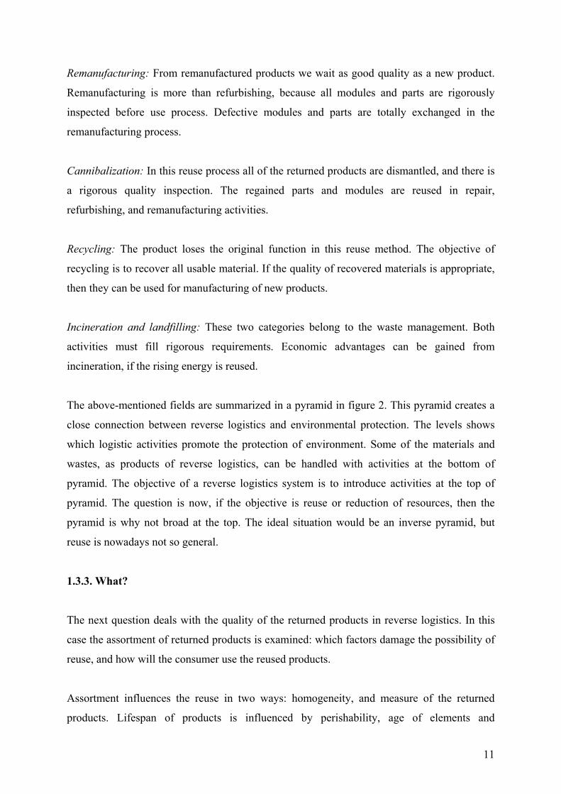
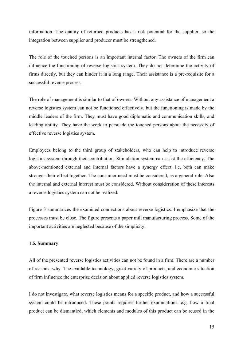
Waste Product Recovery Management
Direct Reuse
7: Incineration 8: Landfilling
5:Cannibalization6: Recycling
2: Repair 3: Refurbishing 4: Remanufacturing
1: Direct reuse/resale
6 5 14
Parts fabrication
Modules assembly
Product assambly
Distribu- tion
Service
Use
2
3
7, 8
Raw materials
Figure 1: Integrated Supply Chain, Source: Thierry et. al. (1995)
10
Resale, Reuse, Redistribution
Repair
Refurbishing
Remanufacturing
Recycling
Incineration, Landfilling
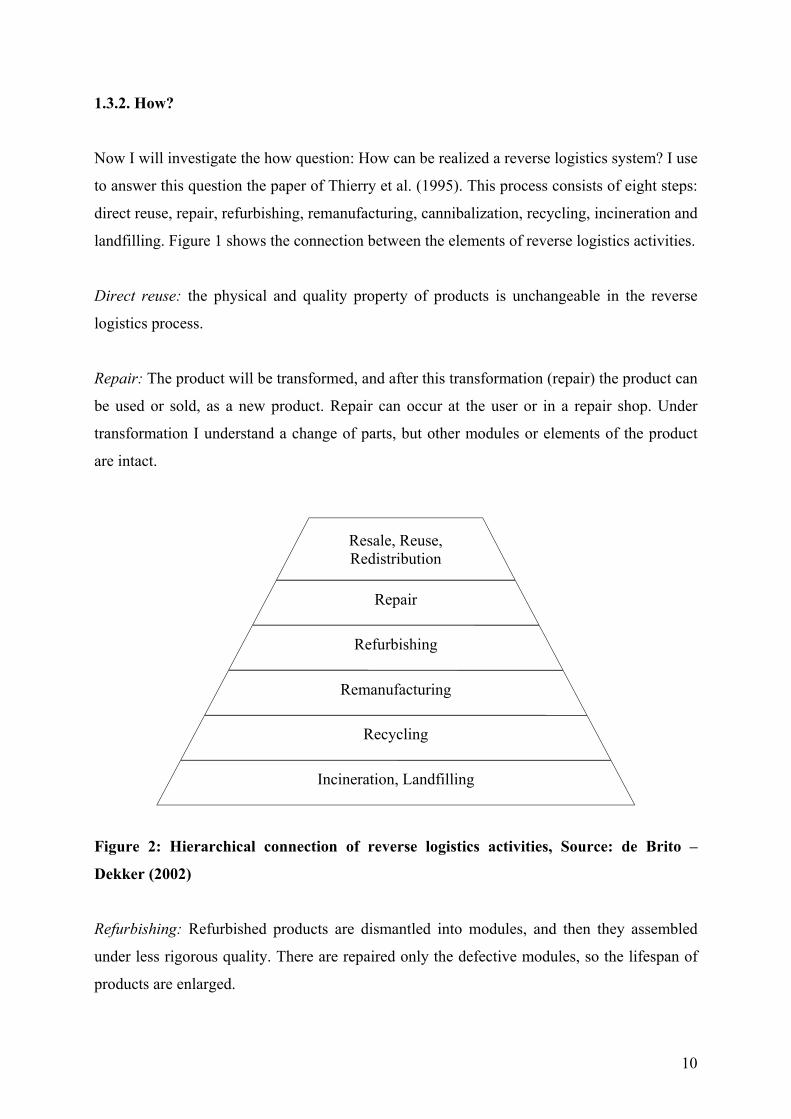
1.3.2. How?
Now I will investigate the how question: How can be realized a reverse logistics system? I use
to answer this question the paper of Thierry et al. (1995). This process consists of eight steps:
direct reuse, repair, refurbishing, remanufacturing, cannibalization, recycling, incineration and
landfilling. Figure 1 shows the connection between the elements of reverse logistics activities.
Direct reuse: the physical and quality property of products is unchangeable in the reverse
logistics process.
Repair: The product will be transformed, and after this transformation (repair) the product can
be used or sold, as a new product. Repair can occur at the user or in a repair shop. Under
transformation I understand a change of parts, but other modules or elements of the product
are intact.
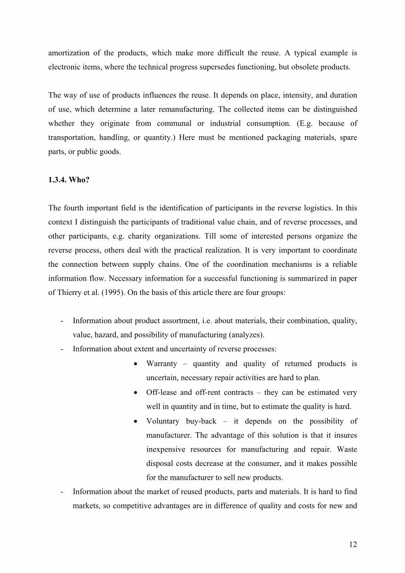
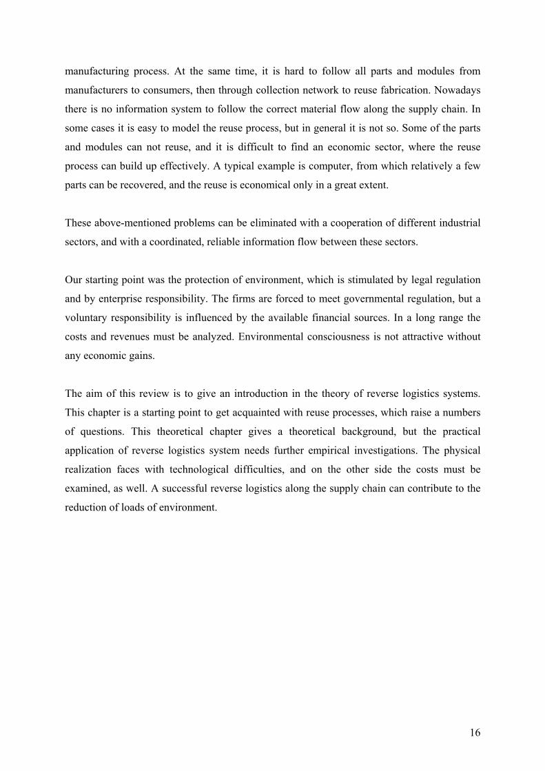
Figure 2: Hierarchical connection of reverse logistics activities, Source: de Brito –
Dekker (2002)
Refurbishing: Refurbished products are dismantled into modules, and then they assembled
under less rigorous quality. There are repaired only the defective modules, so the lifespan of
products are enlarged.
11
Remanufacturing: From remanufactured products we wait as good quality as a new product.
Remanufacturing is more than refurbishing, because all modules and parts are rigorously
inspected before use process. Defective modules and parts are totally exchanged in the
remanufacturing process.
Cannibalization: In this reuse process all of the returned products are dismantled, and there is
a rigorous quality inspection. The regained parts and modules are reused in repair,
refurbishing, and remanufacturing activities.
Recycling: The product loses the original function in this reuse method. The objective of
recycling is to recover all usable material. If the quality of recovered materials is appropriate,
then they can be used for manufacturing of new products.
Incineration and landfilling: These two categories belong to the waste management. Both
activities must fill rigorous requirements. Economic advantages can be gained from
incineration, if the rising energy is reused.
The above-mentioned fields are summarized in a pyramid in figure 2. This pyramid creates a
close connection between reverse logistics and environmental protection. The levels shows
which logistic activities promote the protection of environment. Some of the materials and
wastes, as products of reverse logistics, can be handled with activities at the bottom of
pyramid. The objective of a reverse logistics system is to introduce activities at the top of
pyramid. The question is now, if the objective is reuse or reduction of resources, then the
pyramid is why not broad at the top. The ideal situation would be an inverse pyramid, but
reuse is nowadays not so general.
1.3.3. What?
The next question deals with the quality of the returned products in reverse logistics. In this
case the assortment of returned products is examined: which factors damage the possibility of
reuse, and how will the consumer use the reused products.
Assortment influences the reuse in two ways: homogeneity, and measure of the returned
products. Lifespan of products is influenced by perishability, age of elements and
12
amortization of the products, which make more difficult the reuse. A typical example is
electronic items, where the technical progress supersedes functioning, but obsolete products.
The way of use of products influences the reuse. It depends on place, intensity, and duration
of use, which determine a later remanufacturing. The collected items can be distinguished
whether they originate from communal or industrial consumption. (E.g. because of
transportation, handling, or quantity.) Here must be mentioned packaging materials, spare
parts, or public goods.
1.3.4. Who?
The fourth important field is the identification of participants in the reverse logistics. In this
context I distinguish the participants of traditional value chain, and of reverse processes, and
other participants, e.g. charity organizations. Till some of interested persons organize the
reverse process, others deal with the practical realization. It is very important to coordinate
the connection between supply chains. One of the coordination mechanisms is a reliable
information flow. Necessary information for a successful functioning is summarized in paper
of Thierry et al. (1995). On the basis of this article there are four groups:
- Information about product assortment, i.e. about materials, their combination, quality,
value, hazard, and possibility of manufacturing (analyzes).
- Information about extent and uncertainty of reverse processes:
• Warranty – quantity and quality of returned products is
uncertain, necessary repair activities are hard to plan.
• Off-lease and off-rent contracts – they can be estimated very
well in quantity and in time, but to estimate the quality is hard.
• Voluntary buy-back – it depends on the possibility of
manufacturer. The advantage of this solution is that it insures
inexpensive resources for manufacturing and repair. Waste
disposal costs decrease at the consumer, and it makes possible
for the manufacturer to sell new products.
- Information about the market of reused products, parts and materials. It is hard to find
markets, so competitive advantages are in difference of quality and costs for new and
13
used products. Reuse can be made by the manufacturer, but other firms can realize the
reuse inside and outside supply chain.
- Information about collection of used products and waste disposal. The examination
includes organizations involved in the process, obstacles occurred, quantity of
returned products, and cost-benefit analyzes.
1.4. Stakeholders of reverse logistics
Participants of reverse logistics can be approached in another way. A theoretical background
is supplied in paper of Carter and Ellram (1998), in which there are internal and external
factors that influence reverse logistics.
In general, there are factors within organizations and between organizations, which are
external factors. Internal factors belong interested persons inside of firms, steps for protection
of environment, successful applied business ethics standards, and mainly those persons who
are responsible for the environment friendly corporate philosophy. Also internal influences
have the consumers, supplier, competitors, and government. These four elements are
influenced also by the macro environment with social, political, and economic trends that
touch reverse logistics indirectly.
The listed sectors have a different effect, and they have several interpretations. Among
external factors governmental sector has a most determining influence. It can be accepted
from environmental protection point of view, considering that environmental problems initiate
most of the questions in the European Union. It must be remarked that law forces enterprises,
till other competitors have to consider enterprise competitiveness in the same way. From this
point of view a firm must meet the consumer need under keeping the environmental
regulation of government. Without keeping governmental instruction an enterprise can not
become competitive. There are two views about firm behavior.
14
Supply
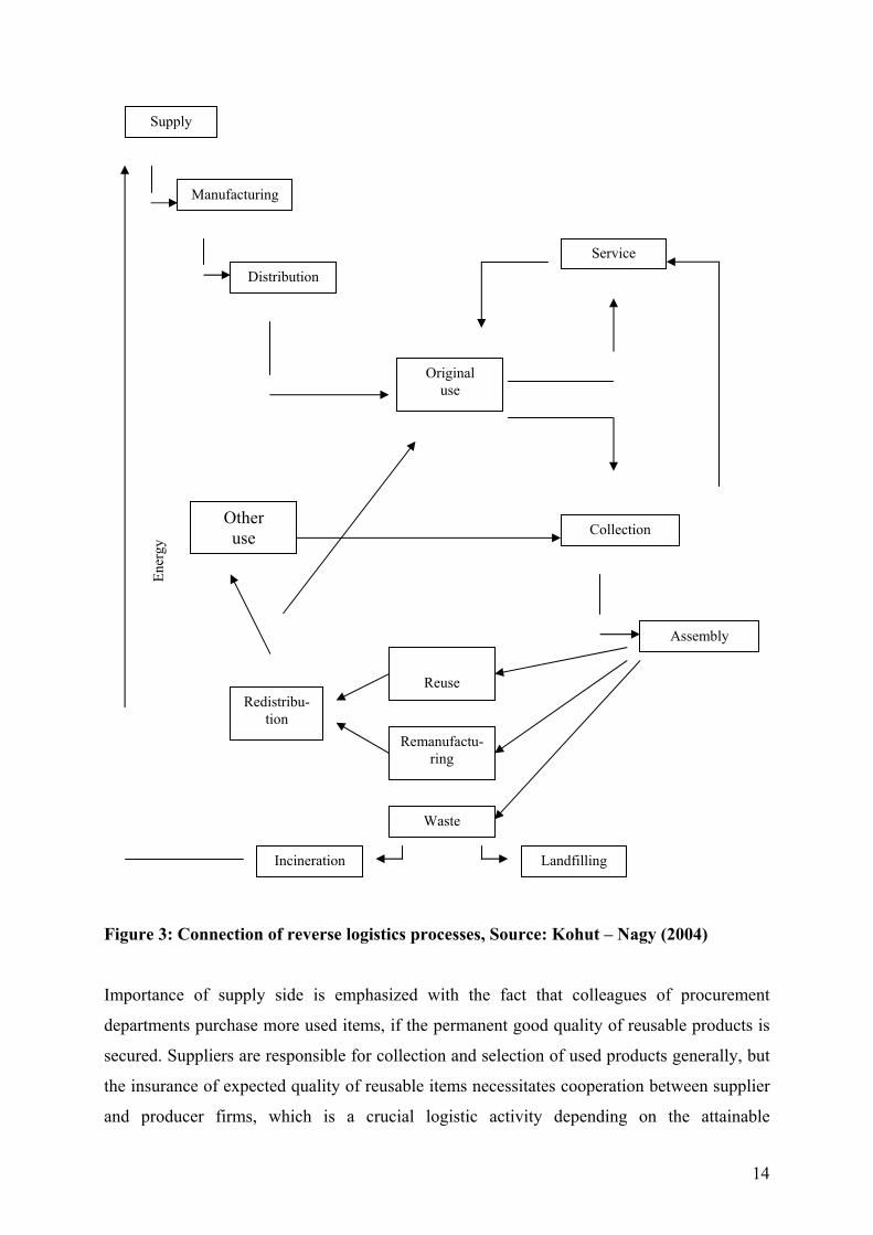
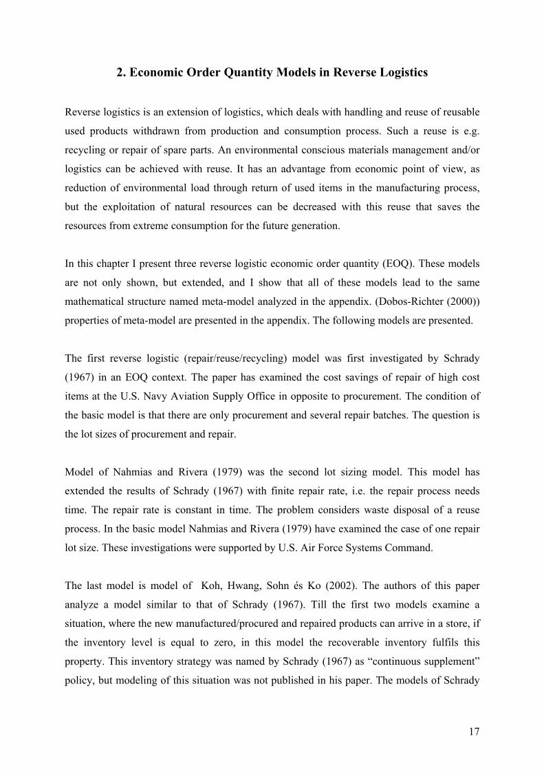
Figure 3: Connection of reverse logistics processes, Source: Kohut – Nagy (2004)
Importance of supply side is emphasized with the fact that colleagues of procurement
departments purchase more used items, if the permanent good quality of reusable products is
secured. Suppliers are responsible for collection and selection of used products generally, but
the insurance of expected quality of reusable items necessitates cooperation between supplier
and producer firms, which is a crucial logistic activity depending on the attainable
Reuse
Original use
Waste
Remanufactu-ring
Distribution
Manufacturing
Collection
Assembly
Service
Incineration Landfilling
Ener
gy
Redistribu-tion
Other use
15
information. The quality of returned products has a risk potential for the supplier, so the
integration between supplier and producer must be strengthened.
The role of the touched persons is an important internal factor. The owners of the firm can
influence the functioning of reverse logistics system. They do not determine the activity of
firms directly, but they can hinder it in a long range. Their assistance is a pre-requisite for a
successful reverse process.
The role of management is similar to that of owners. Without any assistance of management a
reverse logistics system can not be functioned effectively, but the functioning is made by the
middle leaders of the firm. They must have good diplomatic and communication skills, and
leading ability. They have the work to persuade the touched persons about the necessity of
effective reverse logistics system.
Employees belong to the third group of stakeholders, who can help to introduce reverse
logistics system through their contribution. Stimulation system can assist the efficiency. The
above-mentioned external and internal factors have a synergy effect, i.e. both can make
stronger their effect together. The consumer need must be considered, as a general rule. Also
the internal and external interest must be considered. Without consideration of these interests
a reverse logistics system can not be realized.
Figure 3 summarizes the examined connections about reverse logistics. I emphasize that the
processes must be close. The figure presents a paper mill manufacturing process. Some of the
important activities are neglected because of the simplicity.
1.5. Summary
All of the presented reverse logistics activities can not be found in a firm. There are a number
of reasons, why. The available technology, great variety of products, and economic situation
of firm influence the enterprise decision about applied reverse logistics system.
I do not investigate, what reverse logistics means for a specific product, and how a successful
system could be introduced. These points requires further examinations, e.g. how a final
product can be dismantled, which elements and modules of this product can be reused in the
16
manufacturing process. At the same time, it is hard to follow all parts and modules from
manufacturers to consumers, then through collection network to reuse fabrication. Nowadays
there is no information system to follow the correct material flow along the supply chain. In
some cases it is easy to model the reuse process, but in general it is not so. Some of the parts
and modules can not reuse, and it is difficult to find an economic sector, where the reuse
process can build up effectively. A typical example is computer, from which relatively a few
parts can be recovered, and the reuse is economical only in a great extent.
These above-mentioned problems can be eliminated with a cooperation of different industrial
sectors, and with a coordinated, reliable information flow between these sectors.
Our starting point was the protection of environment, which is stimulated by legal regulation
and by enterprise responsibility. The firms are forced to meet governmental regulation, but a
voluntary responsibility is influenced by the available financial sources. In a long range the
costs and revenues must be analyzed. Environmental consciousness is not attractive without
any economic gains.
The aim of this review is to give an introduction in the theory of reverse logistics systems.
This chapter is a starting point to get acquainted with reuse processes, which raise a numbers
of questions. This theoretical chapter gives a theoretical background, but the practical
application of reverse logistics system needs further empirical investigations. The physical
realization faces with technological difficulties, and on the other side the costs must be
examined, as well. A successful reverse logistics along the supply chain can contribute to the
reduction of loads of environment.
17
2. Economic Order Quantity Models in Reverse Logistics
Reverse logistics is an extension of logistics, which deals with handling and reuse of reusable
used products withdrawn from production and consumption process. Such a reuse is e.g.
recycling or repair of spare parts. An environmental conscious materials management and/or
logistics can be achieved with reuse. It has an advantage from economic point of view, as
reduction of environmental load through return of used items in the manufacturing process,
but the exploitation of natural resources can be decreased with this reuse that saves the
resources from extreme consumption for the future generation.
In this chapter I present three reverse logistic economic order quantity (EOQ). These models
are not only shown, but extended, and I show that all of these models lead to the same
mathematical structure named meta-model analyzed in the appendix. (Dobos-Richter (2000))
properties of meta-model are presented in the appendix. The following models are presented.
The first reverse logistic (repair/reuse/recycling) model was first investigated by Schrady
(1967) in an EOQ context. The paper has examined the cost savings of repair of high cost
items at the U.S. Navy Aviation Supply Office in opposite to procurement. The condition of
the basic model is that there are only procurement and several repair batches. The question is
the lot sizes of procurement and repair.
Model of Nahmias and Rivera (1979) was the second lot sizing model. This model has
extended the results of Schrady (1967) with finite repair rate, i.e. the repair process needs
time. The repair rate is constant in time. The problem considers waste disposal of a reuse
process. In the basic model Nahmias and Rivera (1979) have examined the case of one repair
lot size. These investigations were supported by U.S. Air Force Systems Command.
The last model is model of Koh, Hwang, Sohn és Ko (2002). The authors of this paper
analyze a model similar to that of Schrady (1967). Till the first two models examine a
situation, where the new manufactured/procured and repaired products can arrive in a store, if
the inventory level is equal to zero, in this model the recoverable inventory fulfils this
property. This inventory strategy was named by Schrady (1967) as “continuous supplement”
policy, but modeling of this situation was not published in his paper. The models of Schrady
18
(1967) and Nahmias and Rivera (1979) have applied an other inventory policy named
“substitution”. Koh, Hwang, Sohn and Ko (2002) have not expressed the batch sizes, but they
investigate two separate cases: number of purchasing batch is one, and repair batch is one. I
show a new formulation of the model, which treats these two cases in a general model. Koh et
al. (2002), examine an other model. In this model the reuse capacity is not greater than the
demand rate. In my investigation I ignore this type of model.
There is a multi product generalization of EOQ-type reverse logistics models published by
Mabini, Pintelon and Gelders (1998). They have extended the basic model of Schrady (1967)
with capital budget restriction. The examined models have determined the lot sizes, but they
have not taken into account that number of lots is integer, and the sensitivity of return process
from parameters was not investigated.
After this brief overview I summarize the common conditions of these models.
1. The inventory holding policies are known in the models. It means that in an inventory
cycle the inventory status is given and known in time.
2. The demand for new and recovered products is constant and deterministic in time.
3. The return rate of used items is constant and known in time. It is a similar condition to
that of last point.
4. The ordering costs of purchasing and setup costs of repair are known.
5. The inventory holding costs of recovered and new products and holding costs of used
items waiting for repair are known.
6. There is no shortage in store of recovered and new products and store of returned
items.
The first condition defines the inventory holding policy. The variables of these strategies must
be determined in a model, i.e. the lot sizes for new and recovered products, number of batches
for new and used products, and cycle time. The next four conditions are similar to that of
traditional one product EOQ model, i.e. cost structure and demand process. The shortage
situation is excluded with the last condition. Consideration of shortage is not a complicated
mathematical problem, but the aim of this chapter is to give an introduction in the basic
models of EOQ-type reverse logistics models.
19
I present the models in the following sections.
20
2.1. A Reverse Logistics Model with Procurement and Repair
2.1.1. Introduction
A deterministic EOQ-type inventory model for repairable items was first offered by Schrady
(1967). This model can be seen as the first reverse logistics model. His model has examined
the U.S. Naval Supply Systems Command stock holding problem with repairable items. The
repairable items may be scrapped upon a failure, but the products are usually returned from
the user to the overhaul and repair point. The repaired items are sent then to the ready-for-
issue (RFI) inventory to await demand. Based on the feasibility of repair, the items not sent
back are disposed of and they are replaced with new procured products. The returned and not
repaired items are held in a second stock point, i.e. the inventory of non-ready-for-issue
(NRFI) items are awaiting repair at the overhaul and repair point.
Schrady has offered to inventory holding policy to solve problem: the “continuous
supplement” and “substitution” policies. To this last policy he has determined the optimal
procurement and repair quantities. It was assumed that there are only one procurement
quantity (batch size) and more than one repair quantities.
The aim of the paper is to analyze the introduced substitution policy in a general framework.
In this generalization it is allowed a more than one procurement quantity. To solve the
problem we use the meta-model. (See appendix.) Schrady has not investigated the integer
solution for the repair batch number, it is examined now. We will show that the by Schrady
offered solution can be improved in dependence on the recovery (return) rate.
The paper is organized as follows. The next section summarizes the parameters and
functioning of the model. In section 3 we construct the inventory holding cost function of the
model. Then analyzing the total average costs, we determine the optimal procurement/repair
cycle. After eliminating the cycle time we have attained the model in dependence on
procurement and repair batch numbers which leads to the meta-model investigated by the
author, as well. Section 5 presents the basic model of Schrady with one procurement batch.
We will show the optimal integer solution to this model. The following section solves the
generalized model with continuous batch numbers.
21
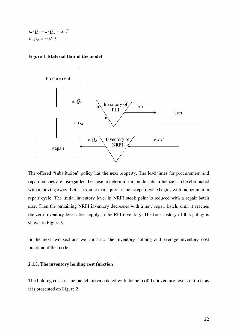
2.1.2. Parameters and functioning of the model
The system contains two inventories. The user’s demand can be satisfied from the RFI
inventory. The demand of the user is constant in time. The RFI inventory is filled up with
procured and repaired items. Shortage is not allowed in this stock point. The procurement and
repair quantities are equal. From the user the repairable items are sent back to the overhaul
and repair point with a constant rate. The repairable items are stored in the NRFI stock point
waiting for repair. After repair products are seen as new and they are sent back to the RFI
inventory. The material flow of the model is depicted in Figure 1. We define the variables and
parameters as follows:
The decision variables of the model:
- QP procurement quantity,
- m number of procurements, m ≥ 1, integer,
- QR repair batch size,
- n number of repair batches, n ≥ 1, integer,
- T procurement/repair cycle time.
Parameters of the model:
- d demand rate, units per unit time,
- r the recovery rate, percent of the demand rate d, the scrap rate is 1-r,
- AP fixed procurement cost, per order,
- AR fixed repair batch induction cost, per batch,
- h1 RFI holding cost, per unit per time,
- h2 NRFI holding cost, per unit per time.
The following equalities show relations between the in- and outflows in the stocking points in
a procurement/repair cycle.
22
TdrQnTdQnQm
R
RP
⋅⋅=⋅⋅=⋅+⋅
Figure 1. Material flow of the model
The offered “substitution” policy has the next property. The lead times for procurement and
repair batches are disregarded, because in deterministic models its influence can be eliminated
with a moving away. Let us assume that a procurement/repair cycle begins with induction of a
repair cycle. The initial inventory level in NRFI stock point is reduced with a repair batch
size. Then the remaining NRFI inventory decreases with a new repair batch, until it reaches
the zero inventory level after supply in the RFI inventory. The time history of this policy is
shown in Figure 3.
In the next two sections we construct the inventory holding and average inventory cost
function of the model.
2.1.3. The inventory holding cost function
The holding costs of the model are calculated with the help of the inventory levels in time, as
it is presented on Figure 2.
n⋅QR
d⋅T
n⋅QR
User
Procurement
Repair
Inventory of RFI
Inventory of NRFI
m⋅QP
r⋅d⋅T
23
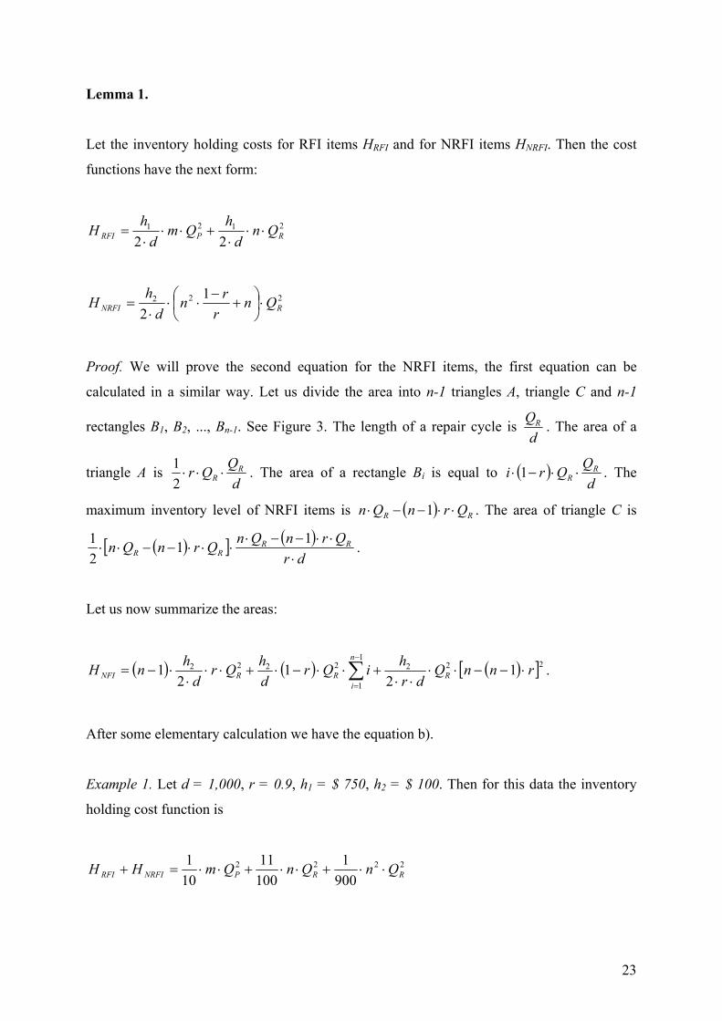
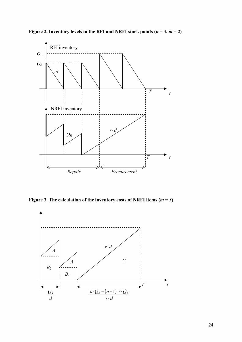
Lemma 1.
Let the inventory holding costs for RFI items HRFI and for NRFI items HNRFI. Then the cost
functions have the next form:
2121
22 RPRFI Qnd
hQmd
hH ⋅⋅⋅
+⋅⋅⋅
=
222 12 RNRFI Qn
rrn
dhH ⋅
+
−⋅⋅
⋅=
Proof. We will prove the second equation for the NRFI items, the first equation can be
calculated in a similar way. Let us divide the area into n-1 triangles A, triangle C and n-1
rectangles B1, B2, ..., Bn-1. See Figure 3. The length of a repair cycle is d
QR . The area of a
triangle A is d
QQr RR ⋅⋅⋅
21 . The area of a rectangle Bi is equal to ( )
dQQri R
R ⋅⋅−⋅ 1 . The
maximum inventory level of NRFI items is ( ) RR QrnQn ⋅⋅−−⋅ 1 . The area of triangle C is
( )[ ] ( )dr
QrnQnQrnQn RRRR ⋅
⋅⋅−−⋅⋅⋅⋅−−⋅⋅
1121 .
Let us now summarize the areas:
( ) ( ) ( )[ ]2221
1
2222 12
12
1 rnnQdr
hiQrdhQr
dhnH R
n
iRRNFI ⋅−−⋅⋅
⋅⋅+⋅⋅−⋅+⋅⋅
⋅⋅−= ∑
−
=
.
After some elementary calculation we have the equation b).
Example 1. Let d = 1,000, r = 0.9, h1 = $ 750, h2 = $ 100. Then for this data the inventory
holding cost function is
2222
9001
10011
101
RRPNRFIRFI QnQnQmHH ⋅⋅+⋅⋅+⋅⋅=+
24
Figure 2. Inventory levels in the RFI and NRFI stock points (n = 3, m = 2)
Figure 3. The calculation of the inventory costs of NRFI items (m = 3)
NRFI inventory
RFI inventory
QR
t
tT
T
r⋅ d
-dQR
QP
Repair Procurement
( )dr
QrnQn RR
⋅⋅⋅−−⋅ 1
dQR
A
A
t T
r⋅ d
B1
B2
C
25
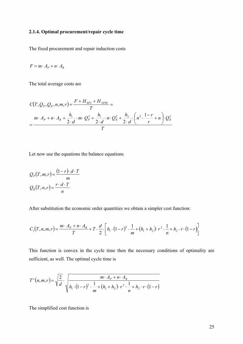
2.1.4. Optimal procurement/repair cycle time
The fixed procurement and repair induction costs
RP AnAmF ⋅+⋅=
The total average costs are
( )
T
Qnr
rnd
hQnd
hQmd
hAnAm
THHF
rmnQQTC
RRPRP
NFRIRFIRP
2222121 1222
,,,,,
⋅
+
−⋅⋅
⋅+⋅⋅
⋅+⋅⋅
⋅+⋅+⋅
=
=++
=
Let now use the equations the balance equations
( ) ( )
( )n
TdrrnTQ
mTdrrmTQ
R
P
⋅⋅=
⋅⋅−=
,,
1,,
After substitution the economic order quantities we obtain a simpler cost function:
( ) ( ) ( ) ( )
−⋅⋅+⋅⋅++⋅−⋅⋅⋅+
⋅+⋅= rrh
nrhh
mrhdT
TAnAmrmnTC RP 1111
2,,, 2
221
211
This function is convex in the cycle time then the necessary conditions of optimality are
sufficient, as well. The optimal cycle time is
( )( ) ( ) ( )rrh
nrhh
mrh
AnAmd
rmnT RPo
−⋅⋅+⋅⋅++⋅−⋅
⋅+⋅⋅=
1111
2,,2
221
21
The simplified cost function is
26
( ) ( ) ( ) ( ) ( )
−⋅⋅+⋅⋅++⋅−⋅⋅⋅+⋅⋅⋅= rrh
nrhh
mrhAnAmdrmnC RP 11112,, 2
221
212
or
( ) ( ) ( ) ( ) ( ) ( )rEnrDmrCmnrB
nmrAdrmnC +⋅+⋅+⋅+⋅⋅⋅= 2,,2
where
( ) ( ) ( ) ( ) ( ) ( )( ) ( ) ( ) ( ) ( ) 2
212
12
22
12
21
11
11
rhhArhArE,rrhArD
,rrhArC,rhArB,rhhArA
RPR
PRP
⋅+⋅+−⋅⋅=−⋅⋅⋅=
−⋅⋅⋅=−⋅⋅=⋅+⋅=
Example 2. Let d = 1,000, r = 0.9, h1 = $ 200, h2 = $ 20, AP = $ 750, AR = $ 100. Then for
this data ( ) ( ) ( ) ( ) ( ) 200,1939.0,1809.0,1359.0,2009.0,650,1339.0 ===== EDCBA
2.1.5. The basic model of Schrady
Schrady has investigated the case with only one procurement batch m = 1. The cost function
of this model is
( ) ( ) ( ) ( ) ( )[ ] ( ) ( )[ ]rErCnrDrBn
rAdr,n,Cr,nC S ++⋅++⋅⋅⋅==1212
The optimal continuous solution for this case is
Lemma 2.
The solution of model of Schrady is
a) if ( ) ( ) ( ) 011 212
221 >−⋅⋅−−⋅⋅⋅−⋅+⋅ rhArrhArhhA RRP ,
27
then ( )
rrhh
hhAA
rrrn
R
Po
−⋅+
+⋅⋅
−=
11
21
21 and
( )( ) ( ) ( )
+⋅⋅+
−⋅+⋅⋅−⋅⋅= 2121 1
12 hhArr
rhhArdr,rnC RPoS
b) if ( ) ( ) ( ) 011 212
221 ≤−⋅⋅−−⋅⋅⋅−⋅+⋅ rhArrhArhhA RRP ,
then ( ) 1=rno and
( )( ) ( ) ( ) ( ) ( )[ ]rrhrhrhhAAdr,rnC RPoS −⋅⋅+−⋅+⋅+⋅+⋅⋅= 112 2
21
221
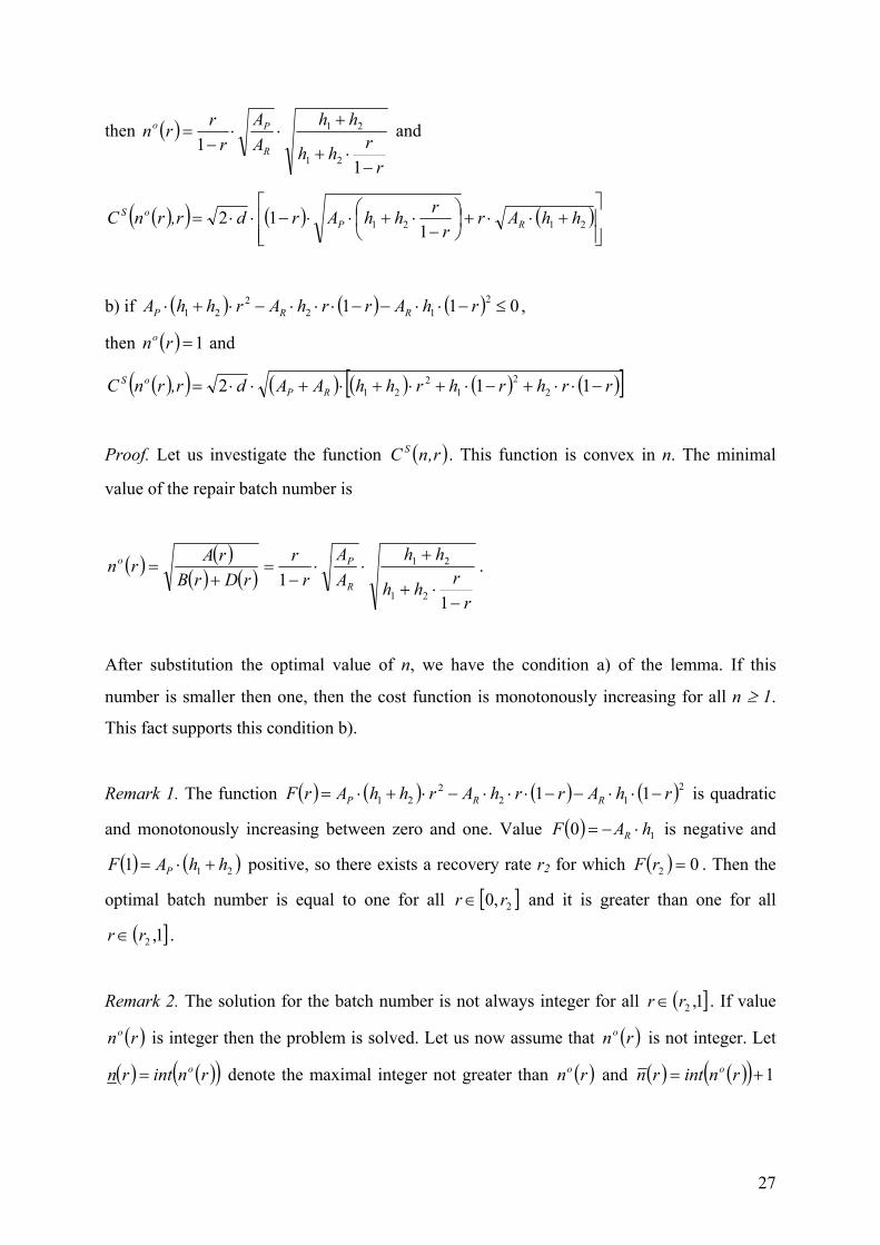
Proof. Let us investigate the function ( )r,nC S . This function is convex in n. The minimal
value of the repair batch number is
( ) ( )( ) ( )
rrhh
hhAA
rr
rDrBrArn
R
Po
−⋅+
+⋅⋅
−=
+=
11
21
21 .
After substitution the optimal value of n, we have the condition a) of the lemma. If this
number is smaller then one, then the cost function is monotonously increasing for all n ≥ 1.
This fact supports this condition b).
Remark 1. The function ( ) ( ) ( ) ( )2122
21 11 rhArrhArhhArF RRP −⋅⋅−−⋅⋅⋅−⋅+⋅= is quadratic
and monotonously increasing between zero and one. Value ( ) 10 hAF R ⋅−= is negative and
( ) ( )211 hhAF P +⋅= positive, so there exists a recovery rate r2 for which ( ) 02 =rF . Then the
optimal batch number is equal to one for all [ ]2,0 rr ∈ and it is greater than one for all
( ]1,2rr ∈ .
Remark 2. The solution for the batch number is not always integer for all ( ]1,2rr ∈ . If value
( )rno is integer then the problem is solved. Let us now assume that ( )rno is not integer. Let
( ) ( )( )rnintrn o= denote the maximal integer not greater than ( )rno and ( ) ( )( ) 1+= rnintrn o
28
the minimal integer not smaller than ( )rno . The optimal integer solution can be determined
from the following relation
( ) ( )( ) ( )( ){ }rnCrnCrn SSoi ,minarg= .
Theorem 1.
The optimal continuous the cycle time and order quantities of model of Schrady are
( ) ( ) ( ) ( )[ ]
( ) ( )( ]
∈−⋅⋅+−⋅
⋅
∈−⋅⋅+⋅++−⋅
+⋅
=1,
112
,011
2
22
21
22
221
21
rrrrhrh
Ad
rrrrhrhhrh
AAd
rTP
RP
o
( )
( ) ( )( ) ( ) ( )
[ ]
( )( ) ( ]
∈⋅+−⋅
−⋅⋅⋅
∈−⋅⋅+⋅++−⋅
−⋅+⋅⋅
=
1,1
12
,011
12
221
22
221
21
2
rrrhrh
rAd
rrrrhrhhrh
rAAd
rQP
RP
oP
and
( )
( )( ) ( ) ( )
[ ]
( ]
∈+⋅⋅
∈−⋅⋅+⋅++−⋅
⋅+⋅⋅
=
1,2
,011
2
221
22
221
21
2
rrhhAd
rrrrhrhhrh
rAAd
rQR
RP
oR
Proof. If [ ]2,0 rr ∈ , i.e. the optimal repair batch number is one, then after substitution we have
the optimal cycle and order quantities. To determine the other case, we use the following
relation
( ) ( )21
2hh
Ar
rnd
)r,rn(T Ro
oo
+⋅⋅= .
29
Substituting the optimal repair batch number and cycle time in balance equations, we get the
results of the theorem.
Schrady in his paper has not analyzed those cases, for which the optimal batch number is even
one. In this formulation we have shown that the solution supplied by Schrady
is limited to the case for ( ]1,2rr ∈ . The method proposed in this paper has the same result for
the economic order quantities, as obtained by Schrady. The optimal cycle time and economic
order quantities for the integer batch number can be calculated with substitution and with
some elementary operations.
Example 3. Let as in Ex. 2. d = 1,000, r = 0.9, h1 = $ 200, h2 = $ 20, AP = $ 750, AR = $ 100.
Then for this data the optimal continuous solution and the switching point r2 are r2 = 0.2316
and 4.357,8$,151.30,828.62,628.0,1,754.18 ====== SoR
oP
ooo CQQyearsTmn .
2.1.6. The optimal number of repair and procurement batches
To minimize the costs in dependence on the batch numbers we apply an auxiliary problem
(meta-model). The problem is
( ) ( ) ( ) ( ) ( ) ( ) minrEnrDmrCmnrB
nmrAdr,n,mC →+⋅+⋅+⋅+⋅⋅⋅= 22
subject to
11 ≥≥ n,m . This problem was extensively studied in papers [1-5]. Based on the mentioned
papers we examine the continuous solution of this model.
Theorem 2.
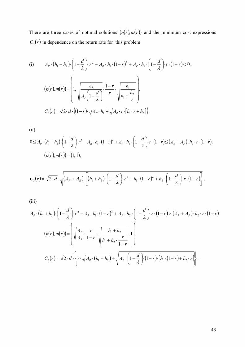
There are three cases of optimal solutions ( ) ( )( )rmrn , and the minimum cost expressions
( )rC3 in dependence on the return rate for this problem
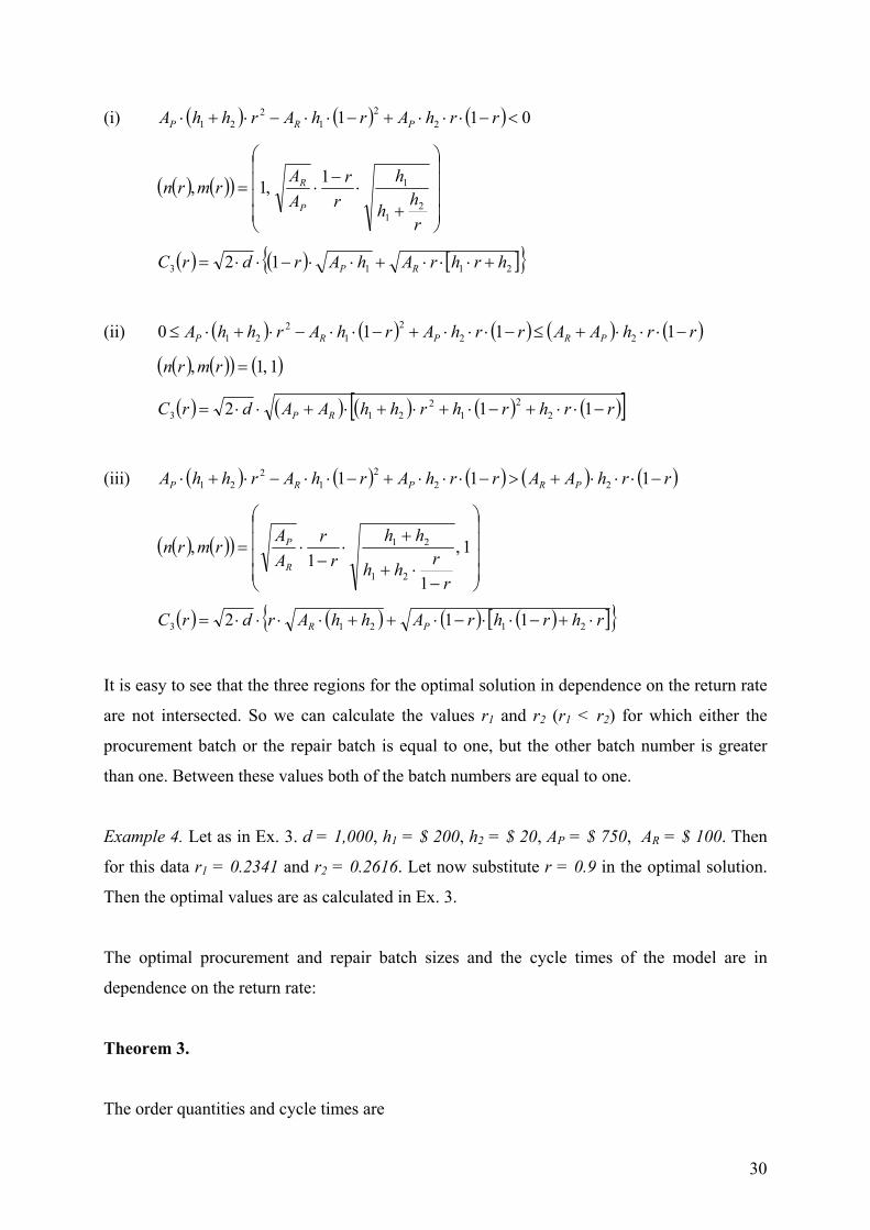
30
(i) ( ) ( ) ( ) 011 22
12
21 <−⋅⋅⋅+−⋅⋅−⋅+⋅ rrhArhArhhA PRP
( ) ( )( )
+⋅
−⋅=
rh
h
hr
rAArmrn
P
R
21
11,1,
( ) ( ) [ ]{ }2113 12 hrhrAhArdrC RP +⋅⋅⋅+⋅⋅−⋅⋅=
(ii) ( ) ( ) ( ) ( ) ( )rrhAArrhArhArhhA PRPRP −⋅⋅⋅+≤−⋅⋅⋅+−⋅⋅−⋅+⋅≤ 1110 222
12
21
( ) ( )( ) ( )1,1, =rmrn
( ) ( ) ( ) ( ) ( )[ ]rrhrhrhhAAdrC RP −⋅⋅+−⋅+⋅+⋅+⋅⋅= 112 22
12
213
(iii) ( ) ( ) ( ) ( ) ( )rrhAArrhArhArhhA PRPRP −⋅⋅⋅+>−⋅⋅⋅+−⋅⋅−⋅+⋅ 111 222
12
21
( ) ( )( )
−⋅+
+⋅
−⋅= 1,
11
,21
21
rrhh
hhr
rAA
rmrnR
P
( ) ( ) ( ) ( )[ ]{ }rhrhrAhhArdrC PR ⋅+−⋅⋅−⋅++⋅⋅⋅⋅= 21213 112
It is easy to see that the three regions for the optimal solution in dependence on the return rate
are not intersected. So we can calculate the values r1 and r2 (r1 < r2) for which either the
procurement batch or the repair batch is equal to one, but the other batch number is greater
than one. Between these values both of the batch numbers are equal to one.
Example 4. Let as in Ex. 3. d = 1,000, h1 = $ 200, h2 = $ 20, AP = $ 750, AR = $ 100. Then
for this data r1 = 0.2341 and r2 = 0.2616. Let now substitute r = 0.9 in the optimal solution.
Then the optimal values are as calculated in Ex. 3.
The optimal procurement and repair batch sizes and the cycle times of the model are in
dependence on the return rate:
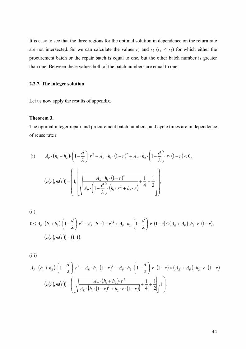
Theorem 3.
The order quantities and cycle times are
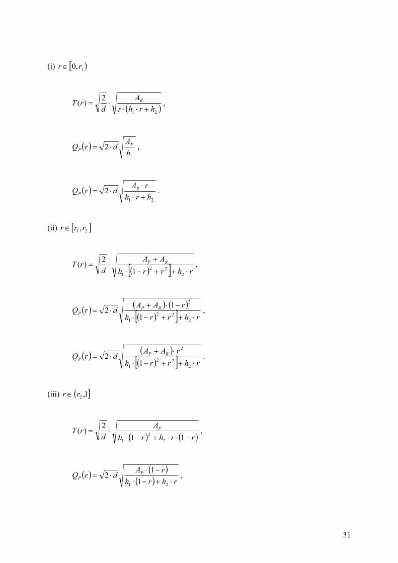
31
(i) [ )1,0 rr ∈
( )21
2)(hrhr
Ad
rT R
+⋅⋅⋅= ,
( )1
2hA
drQ PP ⋅= ,
( )21
2hrh
rAdrQ R
P +⋅⋅
⋅= .
(ii) [ ]21 , rrr ∈
( )[ ] rhrrh
AAd
rT RP
⋅++−⋅+
⋅=2
221 1
2)( ,
( ) ( ) ( )( )[ ] rhrrh
rAAdrQ RPP
⋅++−⋅−⋅+
⋅=2
221
2
112 ,
( ) ( )( )[ ] rhrrh
rAAdrQ RPP
⋅++−⋅⋅+
⋅=2
221
2
12 .
(iii) ( ]1,2rr ∈
( ) ( )rrhrh
Ad
rT P
−⋅⋅+−⋅⋅=
112)(
22
1
,
( ) ( )( ) rhrh
rAdrQ P
P ⋅+−⋅−⋅
⋅=21 1
12 ,
32
( )21
2hh
AdrQ R
P +⋅= .
The proof is easy; we must substitute the continuous batch numbers in the order quantities and
cycle times.
Example 5. Let as in Ex. 3. d = 1,000, r = 0.05, h1 = $ 200, h2 = $ 20, AP = $ 750, AR = $
100. Then for this data the minimal cost for the basic model: CS(0.05) = 17,589.8 and the
minimal cost for the generalized model C(0.05) = 17,002.2. This means a cost saving of 3.5
percent of the total EOQ related costs.
2.1.7. Conclusion
In this paper we have reformulated and solved the model of Schrady. We have shown that for
smaller recovery rate it gives a better solution if the procurement batch number is greater than
one and on the basis of model of Schrady we can obtain a more effective solution for higher
return rate. This result can be interpreted as a generalization of model of Schrady for the case
of more than one procurement batch.
33
2.2. A Model with Purchasing and Finite Repair Rate: Substitution Policy
2.2.1. Introduction
The model of Nahmias and Rivera (1979) is a natural generalization of model of Schrady
(1967). This model takes into account that repair process needs time, i.e. it depends on
capacity.
The model and its solution will be presented in three steps. First I show the functioning of the
repair-procurement process. After that the cost function will be constructed, and then the
optimal decision variables are determined sequentially.
The presented model is an extension of basic model of Nahmias and Rivera (1979). The
authors of this article have allowed only one procurement batch size. I allow in this chapter
more than one procurement. As it will be shown, the number of repair and procurement batch
sizes depends on the return rates.
2.2.2. Parameters and functioning of the model
This inventory system contains two stocking points. The demand of the user is satisfied from
supply depot. Demand is constant in time in a repair and procurement cycle. Supply depot is
filled up from procurement and repair. Shortage is not allowed in this stocking point, so there
are always new products. Procurement and repair batch sizes equal. User of spare parts sends
back the used products in the repair depot with a constant return rate, till they are waiting for
repair. In opposite to the model of Schrady (1967), the capacity of the overhaul department is
finite. It is assumed that repair rate is greater than the demand rate. After repair the spare parts
are sent back to the supply depot, and they are used as newly purchased products. The length
of repair and purchasing lead times are constant, so they do not influence the decision
variables. The material flow of the model is shown in figure 1. The used decision variables
and parameters are similar to that of used by Schrady (1967). This circumstance makes it
easier to compare these models.
The decision variables of the model:
34
- QP procurement quantity,
- m number of procurements, m ≥ 1, integer,
- QR repair batch size,
- n number of repair batches, n ≥ 1, integer,
- T procurement/repair cycle time.
Parameters of the model:
- d demand rate, units per unit time,
- r the recovery rate, percent of the demand rate d, the scrap rate is 1-r,
- λ repair rate per unit time, λ > d,
- AP fixed procurement cost, per order,
- AR fixed repair batch induction cost, per batch,
- h1 holding cost in supply depot, per unit per time,
- h2 holding cost in repair depot, per unit per time.
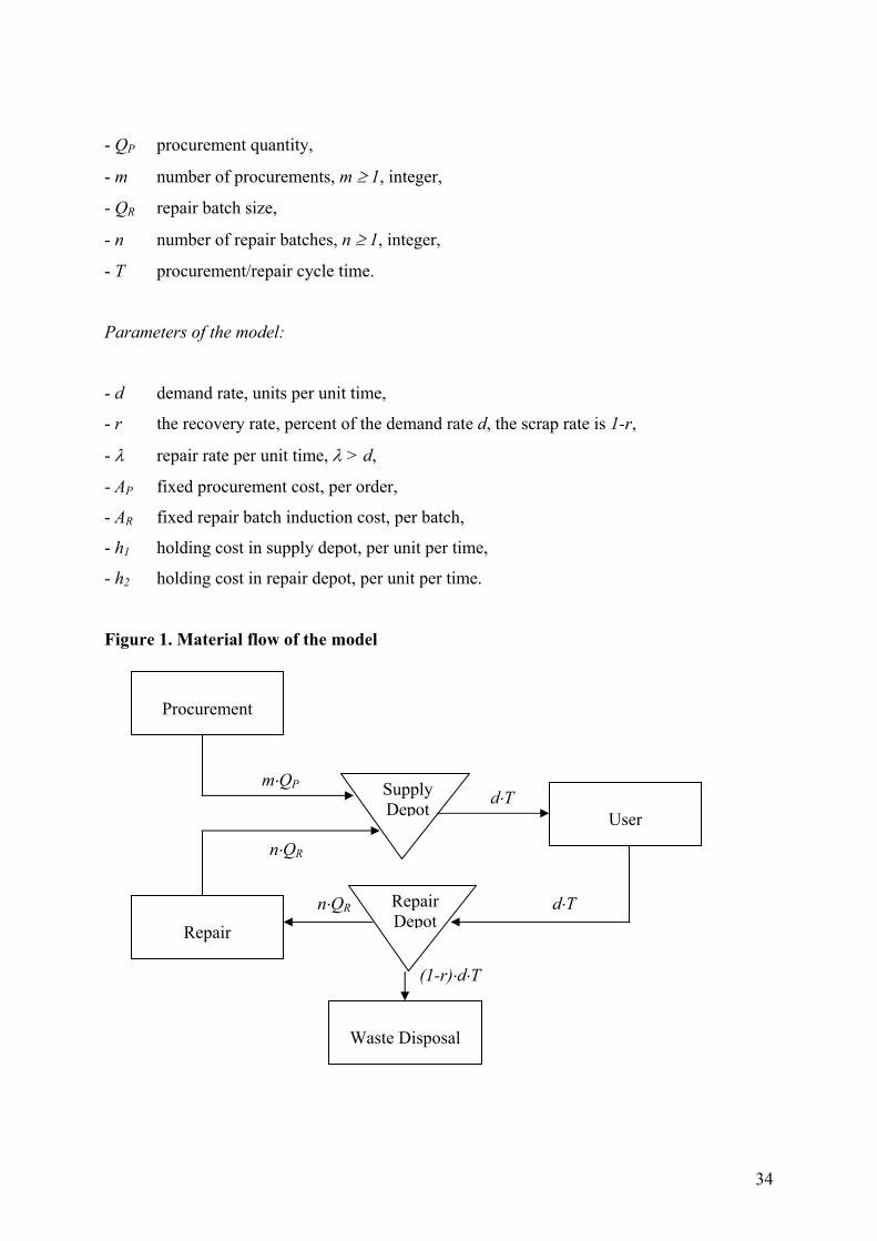
Figure 1. Material flow of the model
(1-r)⋅d⋅T
m⋅QP
n⋅QR
d⋅T
n⋅QR
User
Procurement
Repair
Supply Depot
Repair Depot
d⋅T
Waste Disposal
35
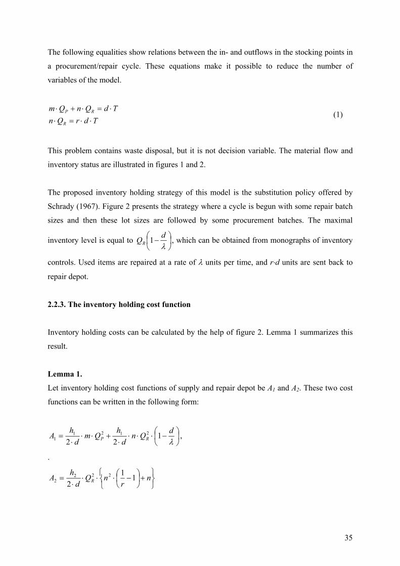
The following equalities show relations between the in- and outflows in the stocking points in
a procurement/repair cycle. These equations make it possible to reduce the number of
variables of the model.
TdrQnTdQnQm
R
RP
⋅⋅=⋅⋅=⋅+⋅
(1)
This problem contains waste disposal, but it is not decision variable. The material flow and
inventory status are illustrated in figures 1 and 2.
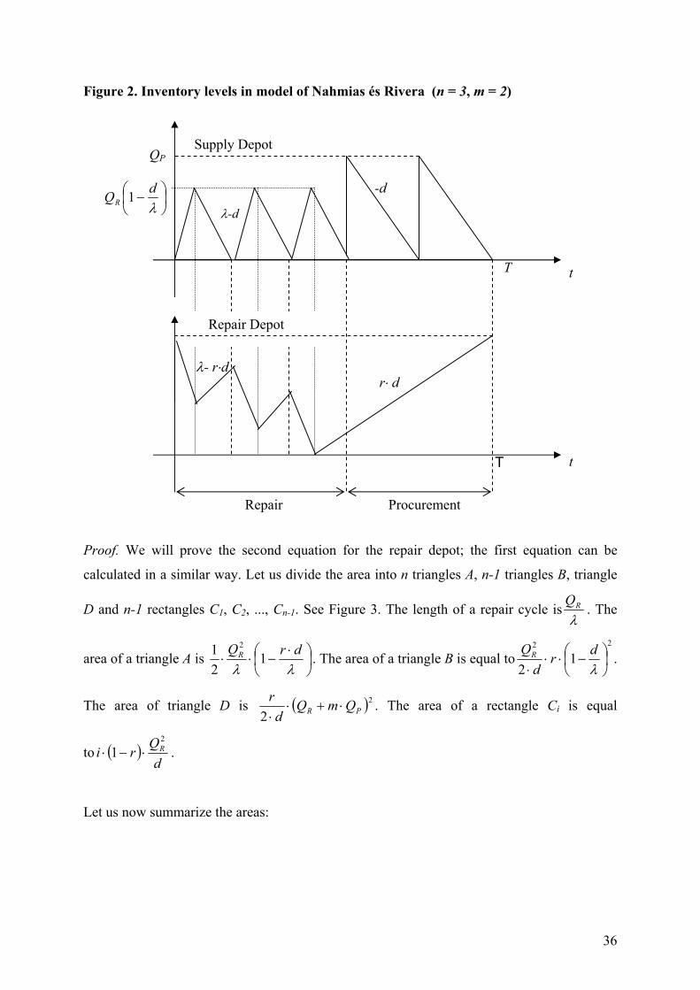
The proposed inventory holding strategy of this model is the substitution policy offered by
Schrady (1967). Figure 2 presents the strategy where a cycle is begun with some repair batch
sizes and then these lot sizes are followed by some procurement batches. The maximal
inventory level is equal to
−
λdQR 1 , which can be obtained from monographs of inventory
controls. Used items are repaired at a rate of λ units per time, and r⋅d units are sent back to
repair depot.
2.2.3. The inventory holding cost function
Inventory holding costs can be calculated by the help of figure 2. Lemma 1 summarizes this
result.
Lemma 1.
Let inventory holding cost functions of supply and repair depot be A1 and A2. These two cost
functions can be written in the following form:
−⋅⋅⋅
⋅+⋅⋅
⋅=
λdQn
dh
Qmd
hA RP 1
222121
1 ,
.
+
−⋅⋅⋅
⋅= n
rnQ
dhA R 11
2222
2
36
Figure 2. Inventory levels in model of Nahmias és Rivera (n = 3, m = 2)
Proof. We will prove the second equation for the repair depot; the first equation can be
calculated in a similar way. Let us divide the area into n triangles A, n-1 triangles B, triangle
D and n-1 rectangles C1, C2, ..., Cn-1. See Figure 3. The length of a repair cycle isλ
RQ . The
area of a triangle A is
⋅−⋅⋅
λλdrQR 1
21 2
. The area of a triangle B is equal to22
12
−⋅⋅
⋅ λdr
dQR .
The area of triangle D is ( )2
2 PR QmQd
r⋅+⋅
⋅. The area of a rectangle Ci is equal
to ( )d
Qri R2
1 ⋅−⋅ .
Let us now summarize the areas:
QP
λ- r⋅d
-d
Supply Depot
t
t T
T
r⋅ d
λ-d
−
λdQR 1
Repair Procurement
Repair Depot
37
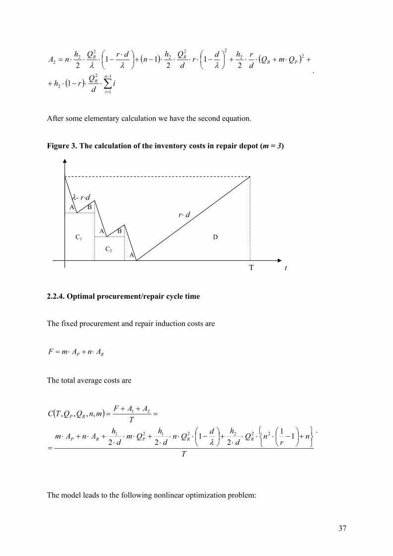
( ) ( )
( ) ∑−
=
⋅⋅−⋅+
+⋅+⋅⋅+
−⋅⋅⋅⋅−+
⋅−⋅⋅⋅=
1
1
2
2
2222
22
22
1
21
211
2n
i
R
PRRR
id
Qrh
QmQdrhdr
dQhndrQhnA
λλλ .
After some elementary calculation we have the second equation.
Figure 3. The calculation of the inventory costs in repair depot (m = 3)
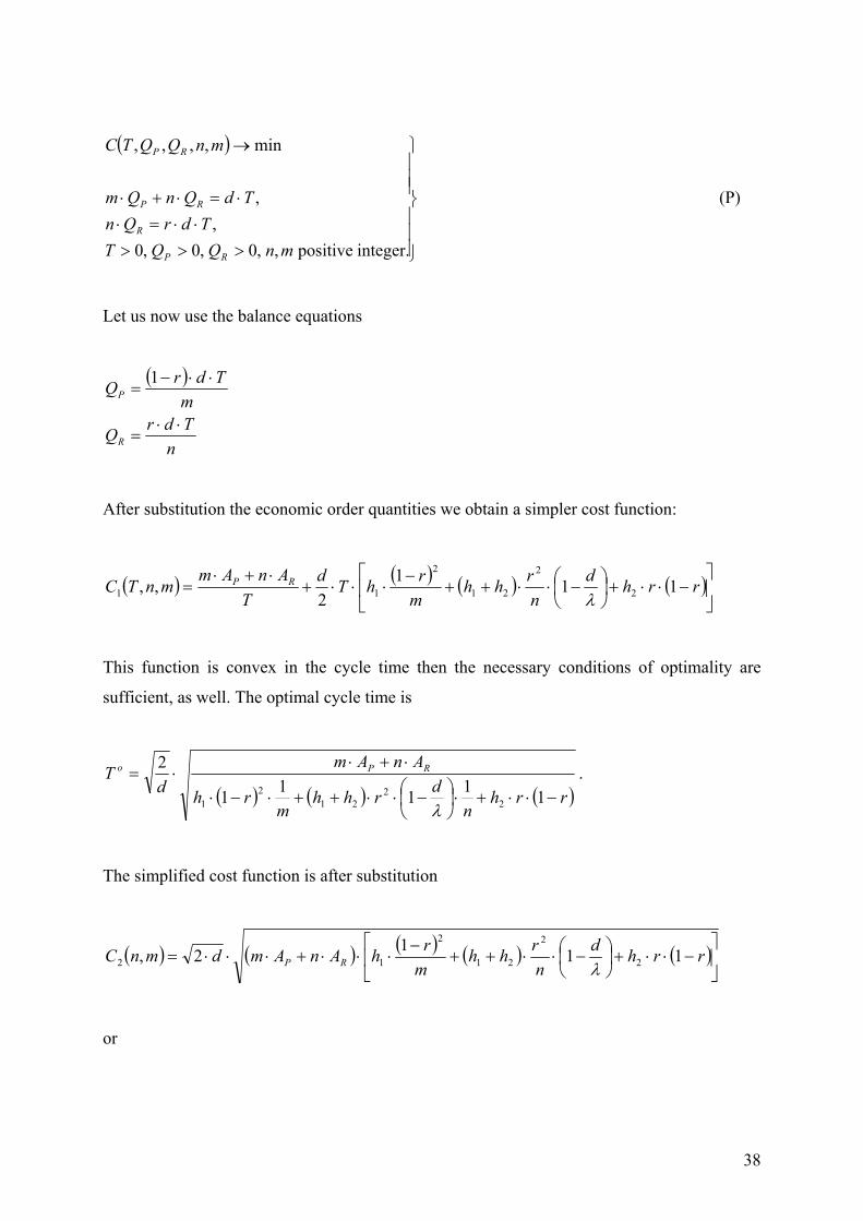
2.2.4. Optimal procurement/repair cycle time
The fixed procurement and repair induction costs are
RP AnAmF ⋅+⋅=
The total average costs are
( )
T
nr
nQd
hdQnd
hQm
dh
AnAm
TAAFmnQQTC
RRPRP
RP
+
−⋅⋅⋅
⋅+
−⋅⋅⋅
⋅+⋅⋅
⋅+⋅+⋅
=
=++
=
112
122
,,,,
2222121
21
λ.
The model leads to the following nonlinear optimization problem:
A
B
BC1
A
A λ- r⋅d
t T
r⋅ d
D
C2
38
( )
>>>⋅⋅=⋅
⋅=⋅+⋅
→
integer.positive,,0,0,0,
,
min,,,,
mnQQTTdrQn
TdQnQm
mnQQTC
RP
R
RP
RP
(P)
Let us now use the balance equations
( )
nTdrQ
mTdrQ
R
P
⋅⋅=
⋅⋅−=
1
After substitution the economic order quantities we obtain a simpler cost function:
( ) ( ) ( ) ( )
−⋅⋅+
−⋅⋅++
−⋅⋅⋅+
⋅+⋅= rrhd
nrhh
mrhTd
TAnAm
mnTC RP 1112
,, 2
2
21
2
11 λ
This function is convex in the cycle time then the necessary conditions of optimality are
sufficient, as well. The optimal cycle time is
( ) ( ) ( )rrhn
drhhm
rh
AnAmd
T RPo
−⋅⋅+⋅
−⋅⋅++⋅−⋅
⋅+⋅⋅=
11111
2
22
212
1 λ
.
The simplified cost function is after substitution
( ) ( ) ( ) ( ) ( )
−⋅⋅+
−⋅⋅++
−⋅⋅⋅+⋅⋅⋅= rrhd
nrhh
mrhAnAmdmnC RP 1112, 2
2
21
2
12 λ
or
39
( ) ( ) ( ) ( ) ( ) ( )rEnrDmrCmnrB
nmrAdmnC +⋅+⋅+⋅+⋅⋅⋅= 2,2 , (2)
where
( ) ( ) ( ) ( ) ( ) ( )
( ) ( ) ( ) ( ) ( ) 221
212
22
12
21
111
,1,1,1
rdhhArhArErrhArD
rrhArCrhArBrdhhArA
RPR
PRP
⋅
−⋅+⋅+−⋅⋅=⋅−⋅⋅=
⋅−⋅⋅=−⋅⋅=⋅
−⋅+⋅=
λ
λ.
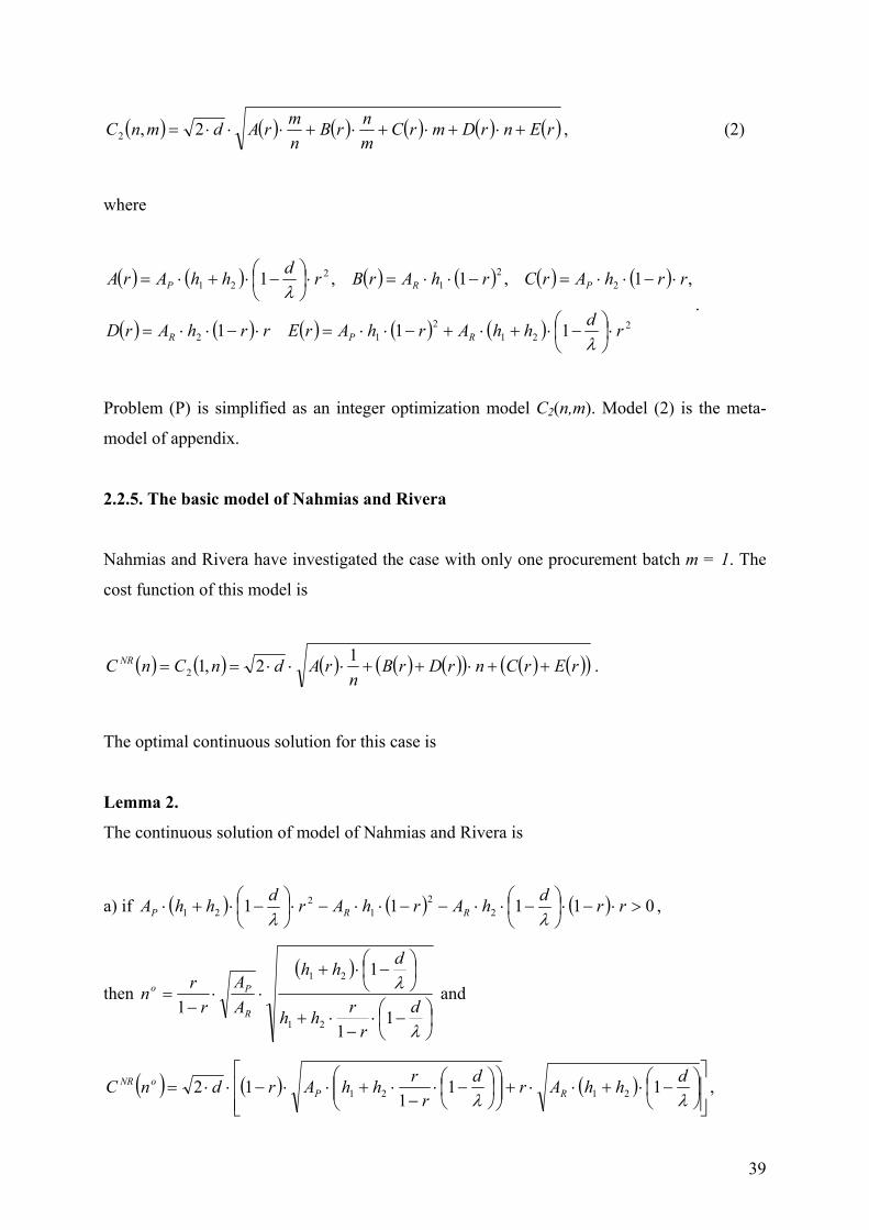
Problem (P) is simplified as an integer optimization model C2(n,m). Model (2) is the meta-
model of appendix.
2.2.5. The basic model of Nahmias and Rivera
Nahmias and Rivera have investigated the case with only one procurement batch m = 1. The
cost function of this model is
( ) ( ) ( ) ( ) ( )( ) ( ) ( )( )rErCnrDrBn
rAdnCnC NR ++⋅++⋅⋅⋅==12,12 .
The optimal continuous solution for this case is
Lemma 2.
The continuous solution of model of Nahmias and Rivera is
a) if ( ) ( ) ( ) 01111 22
12
21 >⋅−⋅
−⋅⋅−−⋅⋅−⋅
−⋅+⋅ rrdhArhArdhhA RRP λλ
,
then ( )
−⋅
−⋅+
−⋅+
⋅⋅−
=
λ
λd
rrhh
dhh
AA
rrn
R
Po
11
1
121
21
and
( ) ( ) ( )
−⋅+⋅⋅+
−⋅
−⋅+⋅⋅−⋅⋅=
λλdhhArd
rrhhArdnC RP
oNR 111
12 2121 ,
40
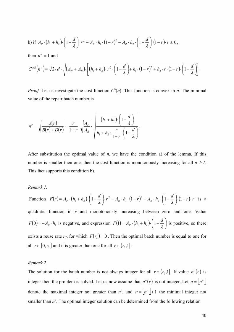
b) if ( ) ( ) ( ) 01111 22
12
21 ≤⋅−⋅
−⋅⋅−−⋅⋅−⋅
−⋅+⋅ rrdhArhArdhhA RRP λλ
,
then 1=on and
( ) ( ) ( ) ( ) ( )
−⋅−⋅⋅+−⋅+
−⋅⋅+⋅+⋅⋅=
λλdrrhrhdrhhAAdnC RP
oNR 11112 22
12
21 .
Proof. Let us investigate the cost function CS(n). This function is convex in n. The minimal
value of the repair batch number is
( )( ) ( )
( )
−⋅
−⋅+
−⋅+
⋅⋅−
=+
=
λ
λd
rrhh
dhh
AA
rr
rDrBrAn
R
Po
11
1
121
21
.
After substitution the optimal value of n, we have the condition a) of the lemma. If this
number is smaller then one, then the cost function is monotonously increasing for all n ≥ 1.
This fact supports this condition b).
Remark 1.
Function ( ) ( ) ( ) ( ) rrdhArhArdhhArF RRP ⋅−⋅
−⋅⋅−−⋅⋅−⋅
−⋅+⋅= 1111 2
21
221 λλ
is a
quadratic function in r and monotonously increasing between zero and one. Value
( ) 10 hAF R ⋅−= is negative, and expression ( ) ( )
−⋅+⋅=
λdhhAF P 11 21 is positive, so there
exists a reuse rate r2, for which ( ) 02 =rF . Then the optimal batch number is equal to one for
all [ ]2,0 rr ∈ and it is greater than one for all ( ]1,2rr ∈ .
Remark 2.
The solution for the batch number is not always integer for all ( ]1,2rr ∈ . If value ( )rno is
integer then the problem is solved. Let us now assume that ( )rno is not integer. Let onn =
denote the maximal integer not greater than no, and 1+= onn the minimal integer not
smaller than no. The optimal integer solution can be determined from the following relation
41
( ) ( ){ }nCnCn NRNRi ,minarg= .
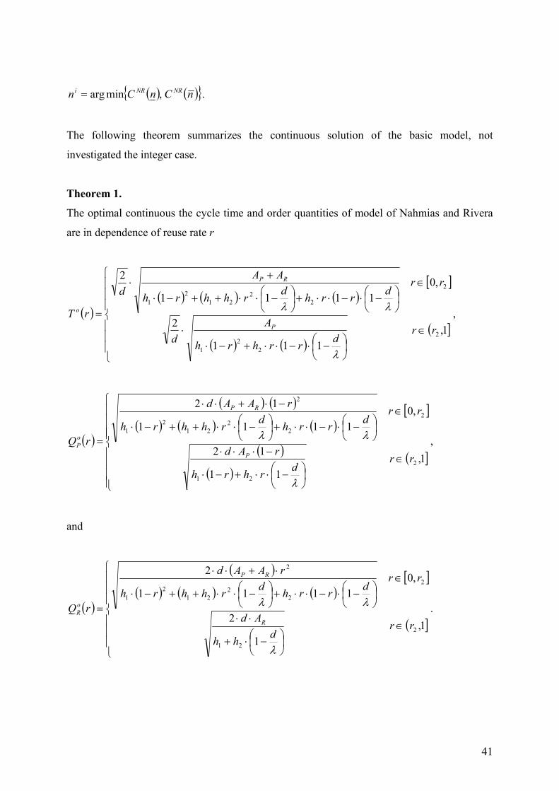
The following theorem summarizes the continuous solution of the basic model, not
investigated the integer case.
Theorem 1.
The optimal continuous the cycle time and order quantities of model of Nahmias and Rivera
are in dependence of reuse rate r
( )( ) ( ) ( )
[ ]
( ) ( )( ]
∈
−⋅−⋅⋅+−⋅
⋅
∈
−⋅−⋅⋅+
−⋅⋅++−⋅
+⋅
=1,
111
2
,01111
2
2
22
1
2
22
212
1
rrdrrhrh
Ad
rrdrrhdrhhrh
AAd
rTP
RP
o
λ
λλ ,
( )
( ) ( )
( ) ( ) ( )[ ]
( )
( )( ]
∈
−⋅⋅+−⋅
−⋅⋅⋅
∈
−⋅−⋅⋅+
−⋅⋅++−⋅
−⋅+⋅⋅
=
1,11
12
,01111
12
2
21
2
22
212
1
2
rrdrhrh
rAd
rrdrrhdrhhrh
rAAd
rQP
RP
oP
λ
λλ ,
and
( )
( )
( ) ( ) ( )[ ]
( ]
∈
−⋅+
⋅⋅
∈
−⋅−⋅⋅+
−⋅⋅++−⋅
⋅+⋅⋅
=1,
1
2
,01111
2
2
21
2
22
212
1
2
rrdhh
Ad
rrdrrhdrhhrh
rAAd
rQR
RP
oR
λ
λλ .
42
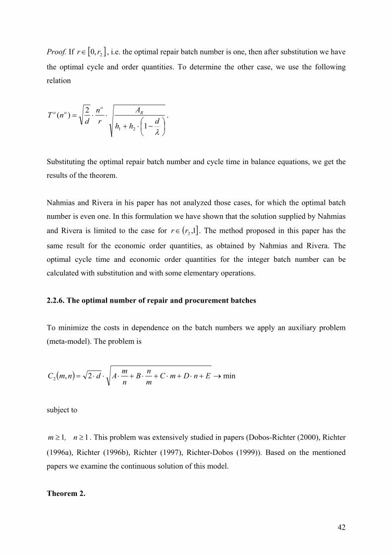
Proof. If [ ]2,0 rr ∈ , i.e. the optimal repair batch number is one, then after substitution we have
the optimal cycle and order quantities. To determine the other case, we use the following
relation
−⋅+
⋅⋅=
λdhh
Ar
nd
nT Ro
oo
1
2)(21
.
Substituting the optimal repair batch number and cycle time in balance equations, we get the
results of the theorem.
Nahmias and Rivera in his paper has not analyzed those cases, for which the optimal batch
number is even one. In this formulation we have shown that the solution supplied by Nahmias
and Rivera is limited to the case for ( ]1,2rr ∈ . The method proposed in this paper has the
same result for the economic order quantities, as obtained by Nahmias and Rivera. The
optimal cycle time and economic order quantities for the integer batch number can be
calculated with substitution and with some elementary operations.
2.2.6. The optimal number of repair and procurement batches
To minimize the costs in dependence on the batch numbers we apply an auxiliary problem
(meta-model). The problem is
( ) min2,2 →+⋅+⋅+⋅+⋅⋅⋅= EnDmCmnB
nmAdnmC
subject to
11 ≥≥ n,m . This problem was extensively studied in papers (Dobos-Richter (2000), Richter
(1996a), Richter (1996b), Richter (1997), Richter-Dobos (1999)). Based on the mentioned
papers we examine the continuous solution of this model.
Theorem 2.
43
There are three cases of optimal solutions ( ) ( )( )rmrn , and the minimum cost expressions
( )rC3 in dependence on the return rate for this problem
(i) ( ) ( ) ( ) 01111 22
12
21 <−⋅⋅
−⋅⋅+−⋅⋅−⋅
−⋅+⋅ rrdhArhArdhhA PRP λλ
,
( ) ( )( )
+⋅
−⋅
−
=
rh
h
hr
rdA
ArmrnP
R
21
11
1,1,
λ
,
( ) ( ) [ ]{ }2113 12 hrhrAhArdrC RP +⋅⋅⋅+⋅⋅−⋅⋅= ,
(ii)
( ) ( ) ( ) ( ) ( )rrhAArrdhArhArdhhA PRPRP −⋅⋅⋅+≤−⋅⋅
−⋅⋅+−⋅⋅−⋅
−⋅+⋅≤ 111110 22
21
221 λλ
,
( ) ( )( ) ( )1,1, =rmrn ,
( ) ( ) ( ) ( ) ( )
−⋅⋅
−⋅+−⋅+⋅
−⋅+⋅+⋅⋅= rrdhrhrdhhAAdrC RP 11112 2
21
2213 λλ
,
(iii)
( ) ( ) ( ) ( ) ( )rrhAArrdhArhArdhhA PRPRP −⋅⋅⋅+>−⋅⋅
−⋅⋅+−⋅⋅−⋅
−⋅+⋅ 11111 22
21
221 λλ
( ) ( )( )
−⋅+
+⋅
−⋅= 1,
11
,21
21
rrhh
hhr
rAArmrn
R
P ,
( ) ( ) ( ) ( )[ ]
⋅+−⋅⋅−⋅
−⋅++⋅⋅⋅⋅= rhrhrdAhhArdrC PR 21213 1112
λ.
44
It is easy to see that the three regions for the optimal solution in dependence on the return rate
are not intersected. So we can calculate the values r1 and r2 (r1 < r2) for which either the
procurement batch or the repair batch is equal to one, but the other batch number is greater
than one. Between these values both of the batch numbers are equal to one.
2.2.7. The integer solution
Let us now apply the results of appendix.
Theorem 3.
The optimal integer repair and procurement batch numbers, and cycle times are in dependence
of reuse rate r
(i) ( ) ( ) ( ) 01111 22
12
21 <−⋅⋅
−⋅⋅+−⋅⋅−⋅
−⋅+⋅ rrdhArhArdhhA PRP λλ
,
( ) ( )( ) ( )
( )
++⋅+⋅⋅
−⋅
−⋅⋅=
21
41
1
1,1,
22
1
21
rhrhdA
rhArmrn
P
R
λ
,
(ii)
( ) ( ) ( ) ( ) ( )rrhAArrdhArhArdhhA PRPRP −⋅⋅⋅+≤−⋅⋅
−⋅⋅+−⋅⋅−⋅
−⋅+⋅≤ 111110 22
21
221 λλ
,
( ) ( )( ) ( )1,1, =rmrn ,
(iii)
( ) ( ) ( ) ( ) ( )rrhAArrdhArhArdhhA PRPRP −⋅⋅⋅+>−⋅⋅
−⋅⋅+−⋅⋅−⋅
−⋅+⋅ 11111 22
21
221 λλ
( ) ( )( ) ( )( ) ( )( )
++
−⋅⋅+−⋅⋅⋅+⋅
= 1,21
41
11,
22
1
221
rrhrhArhhArmrn
R
P .
45
Here function ⋅ denotes the maximal integer not greater than the argument. The proof of the
theorem is easy, with elementary manipulation we get the results. With these results I have
finished the investigation of the model.
2.2.8. Conclusion
The model of Nahmias and Rivera is similar to that of model of Schrady. In this chapter I
have not presented numerical examples. Nahmias and Rivera (1979) have mentioned some
possible extensions in their paper. Such generalizations are e.g. constraints on depot capacity.
The costs of waste disposal and return rate as decision variables are proposed by them.
46
2.3. A Model with Purchasing and Finite Repair Rate: Continuous
Supplement Policy
2.3.1. Introduction
The authors of this model investigate a simple model. The problem is similar to that of
Nahmias and Rivera (1979), but they apply an other inventory holding policy, which is
initiated by Schrady (1967) and called continuous supplement policy instead of substitution
policy. The authors do not express the batch sizes explicitly. The model of Koh et al. (2002)
contains a new formulation for continuous supplement policy. They examine the case of
capacitated remanufacturing rate that is not greater than production and reuse rate, but I do
not analyze that case.
2.3.2. Parameters and functioning of the model
The inventory system contains two stocking points. Demand of users is satisfied from depot
of usable products. Demand is constant in time during reuse cycle. The depot of usable
products is fulfilled from purchase and repair. Shortage is not allowed in this system, so there
are always usable products in depot. The procurement and repair batch sizes are equal. Use
items return from the consumption process with a known return rate. The capacity of repair
department is finite, as it was assumed by Nahmias and Rivers (1979). It is assumed that
repair rate is greater than demand rate that is greater than return rate. After repair the spare
parts are sent back and they are used as new products. Replenishment and repair lead times
are disregarded, because they don not influence the decision variables. The material flow of
this model is depicted on figure 1. Let us now define the decision variables and parameters of
the model.
The decision variables of the model:
- QP procurement batch size,
- m number of procurements, m ≥ 1, integer,
- QR repair batch size,
- n number of repair batches, n ≥ 1, integer,
47
- T procurement/repair cycle time.
Parameters of the model:
- d demand rate, units per unit time,
- r return rate, d > r,
- p production rate, p > d,
- Co fixed procurement cost, per order,
- Cs fixed reuse batch induction cost, per batch,
- Ch2 holding cost of usable products, per unit per time,
- Ch1 holding cost of reusable items, per unit per time.
The inventory levels are presented in figure 2.
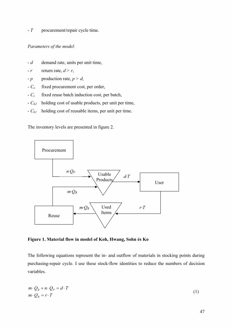
Figure 1. Material flow in model of Koh, Hwang, Sohn és Ko
The following equations represent the in- and outflow of materials in stocking points during
purchasing-repair cycle. I use these stock-flow identities to reduce the numbers of decision
variables.
TrQmTdQnQm
R
PR
⋅=⋅⋅=⋅+⋅
(1)
m⋅QR
d⋅T
m⋅QR
User
Procurement
Reuse
Usable Products
Used Items
n⋅QP
r⋅T
48
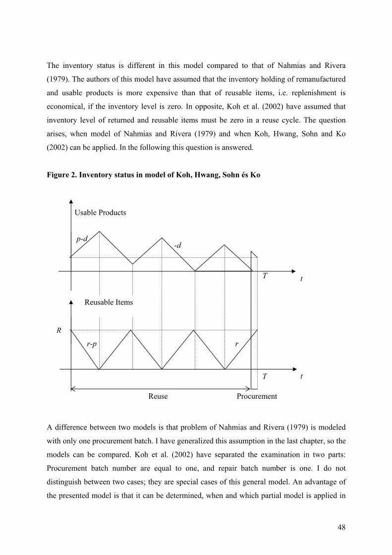
The inventory status is different in this model compared to that of Nahmias and Rivera
(1979). The authors of this model have assumed that the inventory holding of remanufactured
and usable products is more expensive than that of reusable items, i.e. replenishment is
economical, if the inventory level is zero. In opposite, Koh et al. (2002) have assumed that
inventory level of returned and reusable items must be zero in a reuse cycle. The question
arises, when model of Nahmias and Rivera (1979) and when Koh, Hwang, Sohn and Ko
(2002) can be applied. In the following this question is answered.
Figure 2. Inventory status in model of Koh, Hwang, Sohn és Ko
A difference between two models is that problem of Nahmias and Rivera (1979) is modeled
with only one procurement batch. I have generalized this assumption in the last chapter, so the
models can be compared. Koh et al. (2002) have separated the examination in two parts:
Procurement batch number are equal to one, and repair batch number is one. I do not
distinguish between two cases; they are special cases of this general model. An advantage of
the presented model is that it can be determined, when and which partial model is applied in
-d
r-p
R
Usable Products
t
t T
T
r
p-d
Reuse Procurement
Reusable Items
49
dependence of cost parameters and return rates. Of course, these investigations are supported
by the meta-model offered in appendix.
I construct the inventory holding cost function in dependence of decision variables in the next
section. The solution of the model is led to a nonlinear programming problem.
2.3.3. The inventory holding cost function
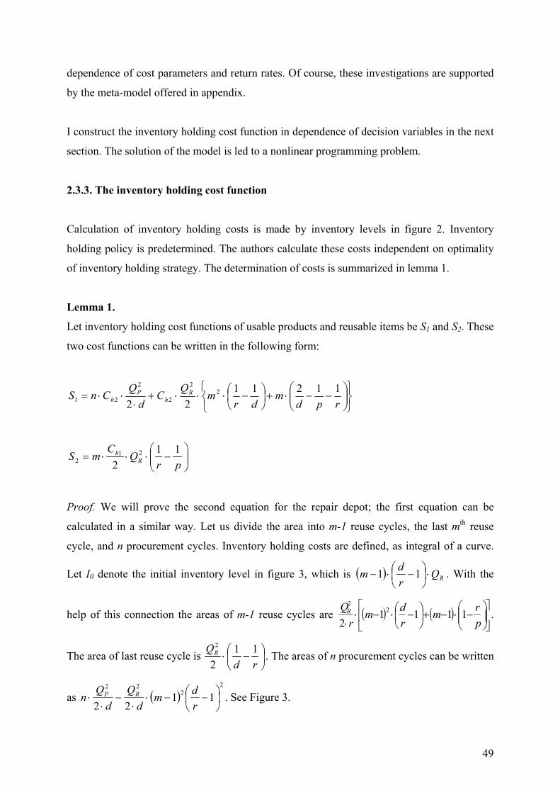
Calculation of inventory holding costs is made by inventory levels in figure 2. Inventory
holding policy is predetermined. The authors calculate these costs independent on optimality
of inventory holding strategy. The determination of costs is summarized in lemma 1.
Lemma 1.
Let inventory holding cost functions of usable products and reusable items be S1 and S2. These
two cost functions can be written in the following form:
−−⋅+
−⋅⋅⋅+
⋅⋅⋅=
rpdm
drm
QC
dQ
CnS Rh
Ph
1121122
22
2
2
21
−⋅⋅⋅=
prQ
CmS R
h 112
212
Proof. We will prove the second equation for the repair depot; the first equation can be
calculated in a similar way. Let us divide the area into m-1 reuse cycles, the last mth reuse
cycle, and n procurement cycles. Inventory holding costs are defined, as integral of a curve.
Let I0 denote the initial inventory level in figure 3, which is ( ) RQrdm ⋅
−⋅− 11 . With the
help of this connection the areas of m-1 reuse cycles are ( ) ( )
−⋅−+
−⋅−⋅
⋅ prm
rdm
rQR 11112
22
.
The area of last reuse cycle is
−⋅
rdQR 112
2
. The areas of n procurement cycles can be written
as ( )2
222
1122
−−⋅
⋅−
⋅⋅
rdm
dQ
dQ
n RP . See Figure 3.
50
Let us now summarize the areas:
( ) ( ) ( )
−−⋅
⋅−
⋅⋅+
−⋅+
−⋅−+
−⋅−⋅
⋅=
22
2222
2
1 1122
112
11112 r
dmd
Qd
Qn
rdQ
prm
rdm
rQ
S RPRR .
After some elementary calculation we have the second equation.
Figure 3. The calculation of the inventory costs of reusable items (m = 3)
2.3.4. Optimal procurement/repair cycle time
The fixed procurement and repair costs are
os CnCmF ⋅+⋅= .
The total average costs are determined in a procurement and repair cycle.
( )
Tpr
QCmCm
Td
QCnCn
Trpd
mdr
mQ
C
TSSF
mnQQTC
Rhs
Pho
Rh
RP
−⋅⋅⋅+⋅
+⋅⋅⋅+⋅
+
−−⋅+
−⋅⋅⋅
=++
=
1122
112112
,,,,
2
1
2
2
22
2
21
.
n procurement
mth reuse m-1 reuses T
I0 -d
Reusable items
t
p-d
51
The model leads to the following nonlinear optimization problem:
The model leads to the following nonlinear optimization problem:
( )
>>>⋅=⋅
⋅=⋅+⋅
→
ű.egészértékpozitív,,0,0,0,
,
min,,,,
mnQQTTrQm
TdQnQm
mnQQTC
RP
R
PR
RP
(P)
Let us now use the balance equations (1) to simplify the problem. Two continuous variables
are substituted in the inventory holding cost function. For the sake of simplicity, let these
variables be the batch sizes. Of course, the batch numbers can be chosen, but this choice
makes more difficult the investigations.
( )
mTrQ
nTrdQ
R
P
⋅=
⋅−=
After substitution the economic order quantities we obtain a simpler cost function. Let the
new cost function denote C1(.).
( )
( )
−⋅⋅+⋅
−⋅+⋅
−⋅⋅+
−−⋅⋅⋅+
+⋅+⋅
=
drrC
ndrdC
mprrC
rpdrCT
TCnCm
mnTC
hh
hh
os
1111111122
,,
22
222
12
2
1
I exclude the cycle time sequentially from this cost function. This function is convex in the
cycle time then the necessary conditions of optimality are sufficient, as well. The optimal
cycle time is
( )( )
−⋅⋅+⋅
−⋅+⋅
−⋅⋅+
−−⋅⋅
⋅+⋅⋅=
drrC
ndrdC
mprrC
rpdrC
CnCmT
hh
hh
oso
1111111122
22
222
12
2
.
52
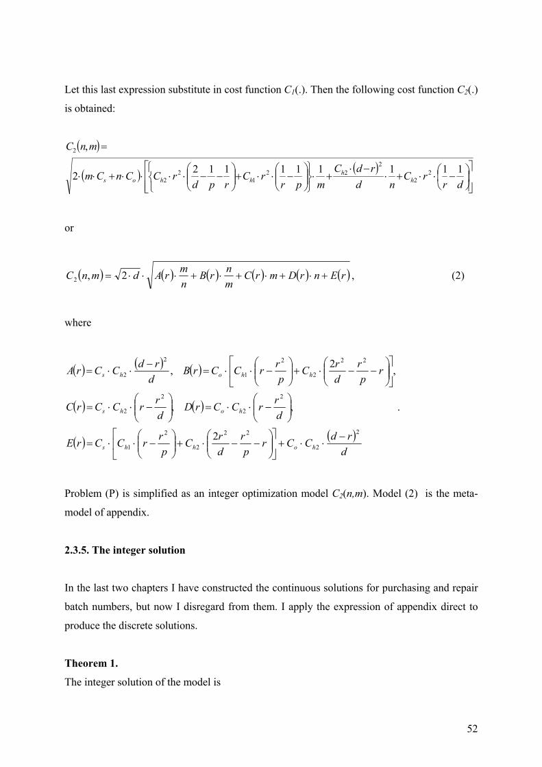
Let this last expression substitute in cost function C1(.). Then the following cost function C2(.)
is obtained:
( )
( ) ( )
−⋅⋅+⋅
−⋅+⋅
−⋅⋅+
−−⋅⋅⋅⋅+⋅⋅
=
drrC
ndrdC
mprrC
rpdrCCnCm
mnC
hh
hhos1111111122
,
22
222
12
2
2
or
( ) ( ) ( ) ( ) ( ) ( )rEnrDmrCmnrB
nmrAdmnC +⋅+⋅+⋅+⋅⋅⋅= 2,2 , (2)
where
( ) ( ) ( )
( ) ( )
( ) ( )d
rdCCrp
rdrC
prrCCrE
drrCCrD
drrCCrC
rp
rdrC
prrCCrB
drdCCrA
hohhs
hohs
hhohs
2
2
22
2
2
1
2
2
2
2
22
2
2
1
2
2
2
,,
,2,
−⋅⋅+
−−⋅+
−⋅⋅=
−⋅⋅=
−⋅⋅=
−−⋅+
−⋅⋅=
−⋅⋅=
.
Problem (P) is simplified as an integer optimization model C2(n,m). Model (2) is the meta-
model of appendix.
2.3.5. The integer solution
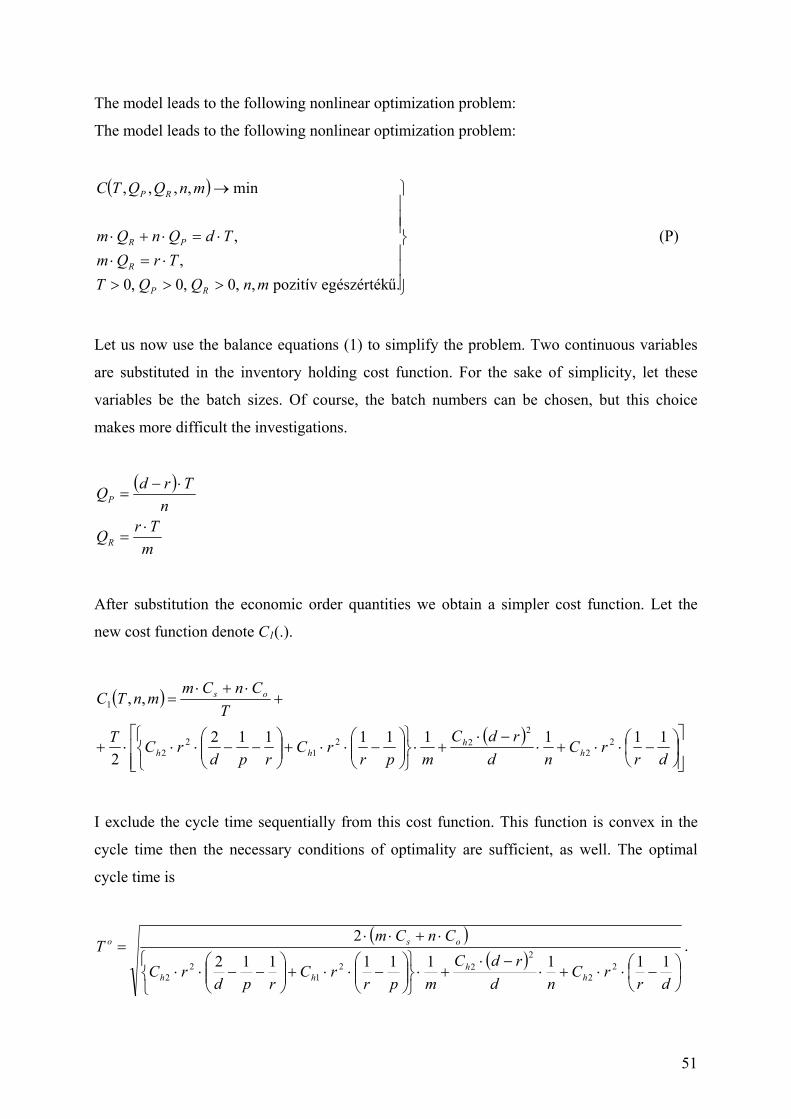
In the last two chapters I have constructed the continuous solutions for purchasing and repair
batch numbers, but now I disregard from them. I apply the expression of appendix direct to
produce the discrete solutions.
Theorem 1.
The integer solution of the model is
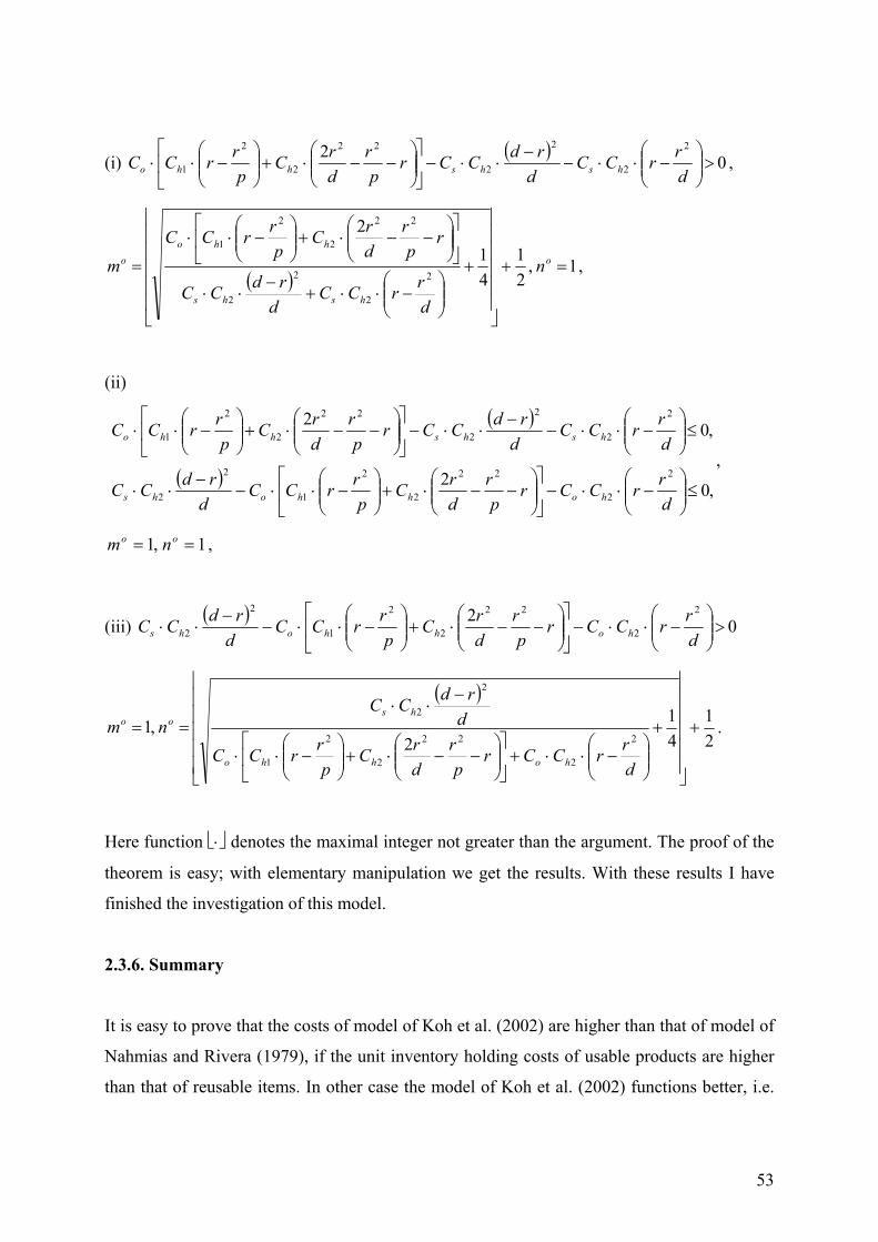
53
(i) ( ) 02 2
2
2
2
22
2
2
1 >
−⋅⋅−
−⋅⋅−
−−⋅+
−⋅⋅
drrCC
drdCCr
pr
drC
prrCC hshshho ,
( )1,
21
41
2
2
2
2
2
22
2
2
1
=+
+
−⋅⋅+
−⋅⋅
−−⋅+
−⋅⋅
= o
hshs
hhoo n
drrCC
drdCC
rp
rdrC
prrCC
m ,
(ii)
( )
( ) ,02
,02
2
2
22
2
2
1
2
2
2
2
2
2
22
2
2
1
≤
−⋅⋅−
−−⋅+
−⋅⋅−
−⋅⋅
≤
−⋅⋅−
−⋅⋅−
−−⋅+
−⋅⋅
drrCCr
pr
drC
prrCC
drdCC
drrCC
drdCCr
pr
drC
prrCC
hohhohs
hshshho
,
1,1 == oo nm ,
(iii) ( ) 02 2
2
22
2
2
1
2
2 >
−⋅⋅−
−−⋅+
−⋅⋅−
−⋅⋅
drrCCr
pr
drC
prrCC
drdCC hohhohs
( )
21
41
2,1
2
2
22
2
2
1
2
2
+
+
−⋅⋅+
−−⋅+
−⋅⋅
−⋅⋅
==
drrCCr
pr
drC
prrCC
drdCC
nm
hohho
hsoo .
Here function ⋅ denotes the maximal integer not greater than the argument. The proof of the
theorem is easy; with elementary manipulation we get the results. With these results I have
finished the investigation of this model.
2.3.6. Summary
It is easy to prove that the costs of model of Koh et al. (2002) are higher than that of model of
Nahmias and Rivera (1979), if the unit inventory holding costs of usable products are higher
than that of reusable items. In other case the model of Koh et al. (2002) functions better, i.e.
54
with lower costs. This fact was proven by Teunter (2004). After some reformulation of model
of Koh et al. (2002) the model becomes problem of a Nahmias and Rivera (1979).
55
3. Inventory Models with Waste Disposal
The objective of the models of last chapter was to minimize the relevant costs, in order to
determine the purchasing and repair lot sizes, and the number of their batches. Cost
minimization is the primary management goal. A second question arises from management
point of view: If the rate of product return is an influenced variable, then how much used
products must be recovered in an inventory cycle. The answer will be looked for this question
in three models of product recovery management.
The three models consist of two parts: first, the optimal lot sizes and number of batches are
determined for reuse/repair and purchasing/manufacturing; secondly, the optimal reuse rate is
determined for known unit manufacturing/purchasing, reuse/repair, and waste disposal costs.
So I define two steps inventory optimization problems.
The first model was initiated by Richter (1996a). The products (containers in this case) are
manufactured in a shop or used containers are repaired in this shop, in order to transport spare
parts in them to an other shop. The empty containers are stored at the second shop, and then
they are collected and sent back to the first manufacturing-repair shop at the end of the
production period. It is decided in the second shop, how many containers are sent back to the
first shop for repair and how many containers are disposed off as waste outside. (Waste
disposal can mean a secondary market of containers.) The following questions arise in this
context: how much percentage of containers are repaired, and lot sizes of manufacturing and
repair, if the aim of decision makers is to minimize the relevant costs.
The next model (Teunter (2001)) investigates a remanufacturing situation. Remanufacturing is
followed by manufacturing in this model. A known part of sold products is returned from the
market, from customers. Waste disposal process begins after ending of remanufacturing, and
after that manufacturing process starts. The question is now, how many items must be
remanufactured from the returned products, and how many items must be disposed of. This
model consists of two parts: minimization of inventory costs, and then determination of reuse
rate.
56
Last, I present a third problem. (Dobos-Richter (2004)) Let us assume that a firm satisfies the
demand from production and recycling. I assume that the production and recycling processes
go on time, so production and recycling rate is finite. The firm purchases the used products to
recycling from market, and the firm can purchase all of its manufactured and used products.
The question is the quantity of product bought back from the market so that the firm
minimizes the total relevant costs, i.e. the sum of EOQ-type and non EOQ-type costs.
The conditions of the three models are common in inventory holding subsystem. These
conditions are found at the end of chapter 2. The conditions must be extended with the
assumption that non EOQ-type costs are linear.
Let us now brief summarize the solution of the models. Since the aim of the models is to
determine the optimal reuse rate, the results are similar for these problems. The optimal reuse
is on the boundary in the optimal solution, i.e. either all of the returned items must be
recovered and the rests are replaced from manufacturing, or the demand is met from
manufacturing and all returned items are disposed off. I prove this property in these models.
And now I present the models.
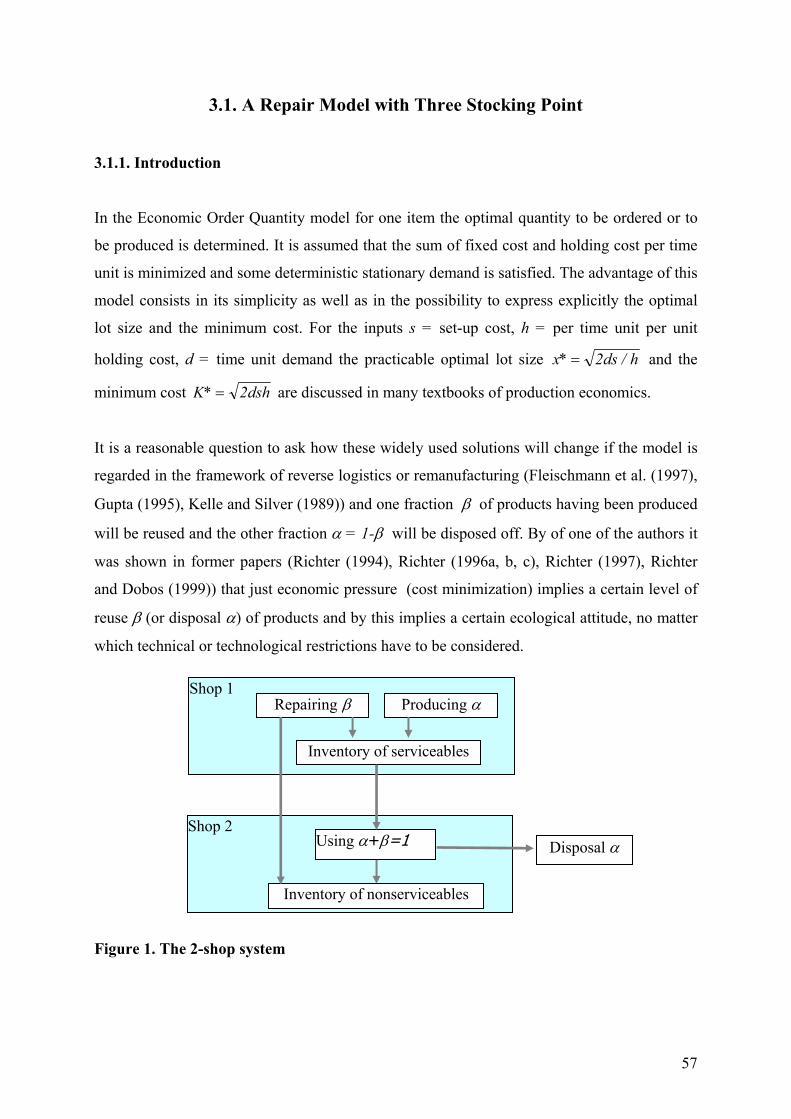
57
3.1. A Repair Model with Three Stocking Point
3.1.1. Introduction
In the Economic Order Quantity model for one item the optimal quantity to be ordered or to
be produced is determined. It is assumed that the sum of fixed cost and holding cost per time
unit is minimized and some deterministic stationary demand is satisfied. The advantage of this
model consists in its simplicity as well as in the possibility to express explicitly the optimal
lot size and the minimum cost. For the inputs s = set-up cost, h = per time unit per unit
holding cost, d = time unit demand the practicable optimal lot size h/ds2*x = and the
minimum cost K dsh* = 2 are discussed in many textbooks of production economics.
It is a reasonable question to ask how these widely used solutions will change if the model is
regarded in the framework of reverse logistics or remanufacturing (Fleischmann et al. (1997),
Gupta (1995), Kelle and Silver (1989)) and one fraction β of products having been produced
will be reused and the other fraction α = 1-β will be disposed off. By of one of the authors it
was shown in former papers (Richter (1994), Richter (1996a, b, c), Richter (1997), Richter
and Dobos (1999)) that just economic pressure (cost minimization) implies a certain level of
reuse β (or disposal α) of products and by this implies a certain ecological attitude, no matter
which technical or technological restrictions have to be considered.
Figure 1. The 2-shop system
Shop 1 Repairing β Producing α
Inventory of serviceables
Shop 2 Using α+β=1
Inventory of nonserviceables
Disposal α
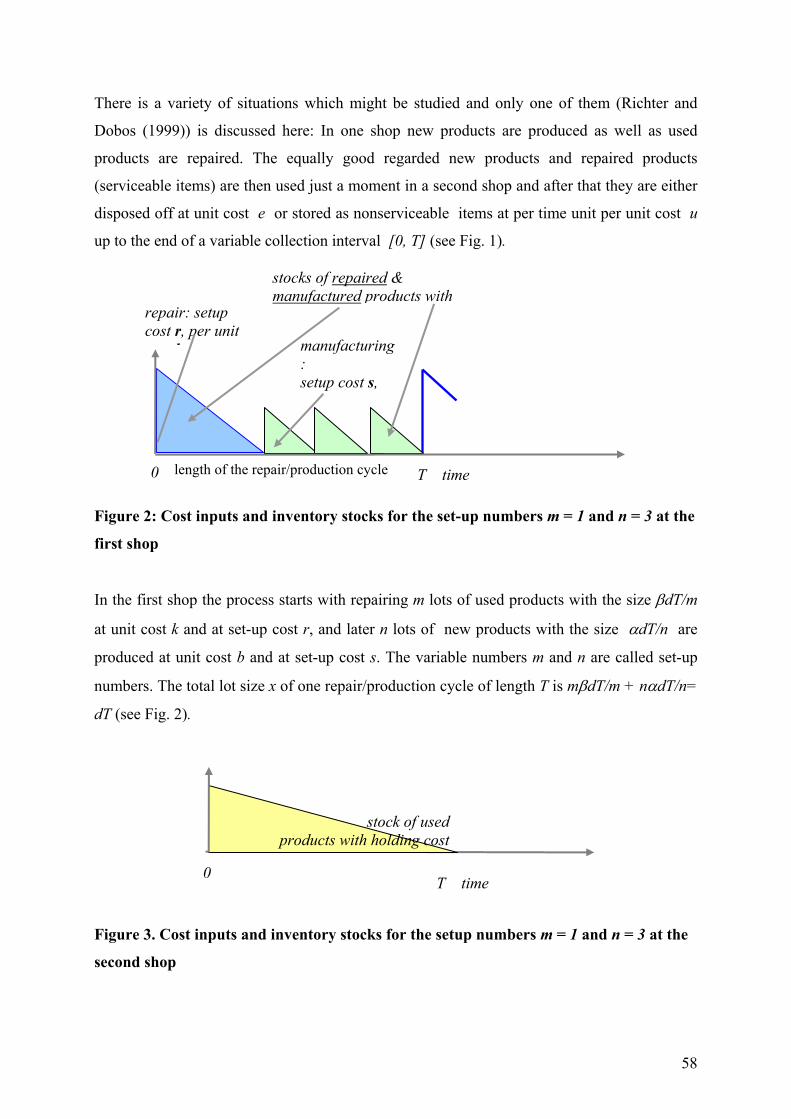
58
There is a variety of situations which might be studied and only one of them (Richter and
Dobos (1999)) is discussed here: In one shop new products are produced as well as used
products are repaired. The equally good regarded new products and repaired products
(serviceable items) are then used just a moment in a second shop and after that they are either
disposed off at unit cost e or stored as nonserviceable items at per time unit per unit cost u
up to the end of a variable collection interval [0, T] (see Fig. 1).
Figure 2: Cost inputs and inventory stocks for the set-up numbers m = 1 and n = 3 at the
first shop
In the first shop the process starts with repairing m lots of used products with the size βdT/m
at unit cost k and at set-up cost r, and later n lots of new products with the size αdT/n are
produced at unit cost b and at set-up cost s. The variable numbers m and n are called set-up
numbers. The total lot size x of one repair/production cycle of length T is mβdT/m + nαdT/n=
dT (see Fig. 2).
Figure 3. Cost inputs and inventory stocks for the setup numbers m = 1 and n = 3 at the
second shop
0 T time
stock of used products with holding cost
stocks of repaired & manufactured products with
repair: setup cost r, per unit
t k manufacturing: setup cost s,
0 T time length of the repair/production cycle
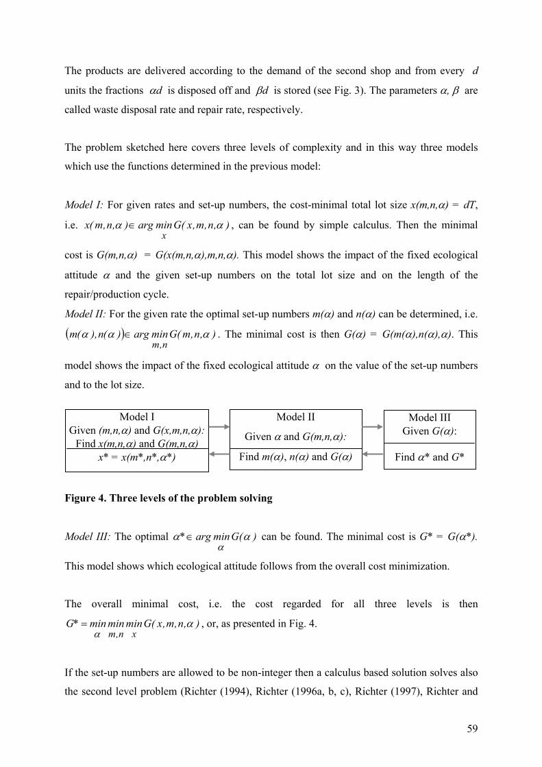
59
The products are delivered according to the demand of the second shop and from every d
units the fractions αd is disposed off and βd is stored (see Fig. 3). The parameters α, β are
called waste disposal rate and repair rate, respectively.
The problem sketched here covers three levels of complexity and in this way three models
which use the functions determined in the previous model:
Model I: For given rates and set-up numbers, the cost-minimal total lot size x(m,n,α) = dT,
i.e. ),n,m,x(Gminarg),n,m(xx
αα ∈ , can be found by simple calculus. Then the minimal
cost is G(m,n,α) = G(x(m,n,α),m,n,α). This model shows the impact of the fixed ecological
attitude α and the given set-up numbers on the total lot size and on the length of the
repair/production cycle.
Model II: For the given rate the optimal set-up numbers m(α) and n(α) can be determined, i.e.
( ) ),n,m(Gminarg)(n),(mn,m
ααα ∈ . The minimal cost is then G(α) = G(m(α),n(α),α). This
model shows the impact of the fixed ecological attitude α on the value of the set-up numbers
and to the lot size.
Figure 4. Three levels of the problem solving
Model III: The optimal )(Gminarg* ααα
∈ can be found. The minimal cost is G* = G(α*).
This model shows which ecological attitude follows from the overall cost minimization.
The overall minimal cost, i.e. the cost regarded for all three levels is then
),n,m,x(Gminminmin*Gxn,m
αα
= , or, as presented in Fig. 4.
If the set-up numbers are allowed to be non-integer then a calculus based solution solves also
the second level problem (Richter (1994), Richter (1996a, b, c), Richter (1997), Richter and
Model I Given (m,n,α) and G(x,m,n,α):
Find x(m,n,α) and G(m,n,α) x* = x(m*,n*,α*)
Model III Given G(α):
Find α* and G*
Model II
Given α and G(m,n,α):
Find m(α), n(α) and G(α)
60
Dobos (1999))). The function G(m,n,α) has been separated in (Richter (1996a, b, c), Richter
(1997), Richter and Dobos (1999))) into G(m,n,α) = K(m,n,α) + R(α) where K(m,n,α) is the
so called EOQ-related cost and R(α) = d(α(e+b)+(1-α)k) expresses the EOQ-independent
per time unit repair, manufacturing and disposal cost. As long as model I /II are regarded
where α is fixed, the cost R(α) does not have impact on the minimum and the main question
is the determination of the optimal solutions for K(m,n,α). This remains also true for model III
because of the linearity of R(α).
Here, however, it will be asked what happens if the numbers m and n must be integers. In
papers Richter (1994), Richter (1996a, b, c), Richter (1997), Richter and Dobos (1999)) the
non-integer problem of minimizing the cost function G(m,n,α), i. e. the non-integer problem
of minimizing the cost function K(m,n,α) on m,n ≥ 1, has been solved by analyzing a special
fractional program S(m,n) → min, subject to m,n ≥ 1.
Similarly, the integer problem
G(m,n,α) → min [= G(α)], m,n ∈ {1,2,...} (1)
K(m,n,α) → min [= K(α)], m,n ∈ {1,2,...}
can be solved if a solution is found for minimizing that auxiliary function S(m,n) on m,n ∈
{1,2,...}. In paper Richter and Dobos (1999) the integer problem (1) has been analyzed and it
was stated that
• the optimal solution is boundary, i.e. one of the lot numbers equals one under certain
conditions,
• some relative error for the non-optimality of boundary solutions can be given,
• the minimum cost functions are partly convex and partly concave under various
conditions and
• these results can be applied to the initial models I-III.
In this papers all properties from paper of Richter (1997) will be proved now, will be
discussed in greater detail and an example will be provided that shows that the optimal integer
solution is not necessarily boundary.
The auxiliary function S(m,n) has been derived in papers of Richter (1994), Richter (1996a, b,
c), Richter (1997), Richter and Dobos (1999)) from the following cost function
61
K(m,n,α) = ( )
++−++ 2
22
)()(2 βββα um
uhn
hnsmrd , (2)
which covers the EOQ-related cost from G(m,n,α). Due to monotonicity considerations the
function S(m,n,α) = (mr+ns)(hα2/n+ (h-u)β2/m+u(β+β2)), (3)
can be analyzed instead of (2). For both functions the relationship K(m,n,α)=
2d S m n⋅ ( , , )α holds.
The parameters in the function (3) can be replaced by
A = rhα2, B = s(h-u) β2, C = ru(β+β²), D= su(β+β²), E = shα2+r(h-u) β2 (4)
and, thus, the function
S m n A mn
B nm
Cm Dn E( , ) = + + + + , (5)
appears. If the minimum of the function (5) on m,n ∈ {1,2,...} is determined then also the
problem K(m,n,α) → min on m,n ∈ {1,2,...} is solved, and, since G(m,n,α) = K(m,n,α) +
R(α). Therefore, it will be asked in the next section, which solution can be found for the
problem of minimizing the function (5) on the set of positive integers.
3.1.2. Application to the repair and waste disposal model
3.1.2.1. The optimal solution
Due to paper of Richter (1997) the relations A, C, D, B+D, E > 0 hold and the results of the
Lemma 4 of appendix are to be applied.
Theorem 1 (Richter (1997)): The continuous optimal solution for minimizing the function
(2) is
(i) {h > u} ∧ {s(h-u) β² ≥ r ( )α β β² h+ u( )1+ } ⇒ m(α) = β ( )s h u
r u( )
( )−
+α β β² h+ 1, n(α)= 1,
(ii) rhα²-suβ(1+β) ≤ s(h-u)β² ≤ r( )α β β² h+ u( )1+ ⇒ (m(α),n(α)) = (1,1),
(iii) α²rh ≥ sβ β( )h u+ ⇒ m(α) =1, n(α) = α rhs h uβ β( )+
,
62
According to the cases (i) - (iii) the region (0,1) is separated into three subregions and it is
clear that the problem of finding an optimal integer solution needs special attention only for
α ∈ (0, α1) ∪ (α2,1). Therefore the two cases (i) and (iii) will be studied in detail and the
results of Theorem 3 from [13] will be extended.
Lemma 1: (i) 49A ≤ 527C holds if α ≤ α3 = 105449 1054
uh u+
and 49h-527u > 0 and α3 = 2/3 in
the opposite case and (iii) 49B ≤ 527D holds if α ≥ α4 = 49 110349 576
h uh u−−
and 49h > 576u and
for every α in the opposite case.
Proof: (i) The inequality holds if and only if 49hα2 ≤ 527uβ(1+β) or (49h-527u)α2 +1571uα
≤ 1054u. Since u > 0 and α ≥ α2 holds the inequality is satisfied at most by α ≤ α3.
(iii) The other inequality holds if and only if 49(h-u)β ≤ 527u(1+β) is fulfilled or (49h-576u)β
≤ 527u. If 49h ≤ 576u then that inequality holds for every β and α. In the other case the
inequalities β ≤ 527u/(49h-576u) and α ≥ α4 hold.
Lemma 2: The boundaries of the two sets α1 and α2 fulfill:
(i) α1 ≤ s h u rus h u r h u
( )( ) ( )
− −− + −
22
if s(h-u) > r(h+u) and α1 ≤ h uh u−−2
in the other case.
(iii) α2 ≥ s h u
s h u hr( )
( )+
+ + if r > s and α2 ≥
h uh u++2
if r ≤ s
Proof: (i) The relation B ≥ A+C holds if h > u and β²s(h-u) ≥ r ( )α β β² h+ u( )1+ hold. After
some transformation the inequality β2[s(h-u) - r(h+u)]+ βr(2h-u) ≥ rh has to be analyzed and
the formulas under (i) appears.
(iii) The relation A ≥ B+D implies that rhα2 ≥ s(1-α)[h(1-α)+u] and that
α2h(r-s)+ αs(2h+u) ≥ s(h+u). (6)
If s=r the statement holds obviously. If r > s then
α[hr+ s(h+u)] = αh(r-s)+ αs(2h+u) ≥ α2h(r-s)+ αs(2h+u)
and every α satisfying (11) satisfies also α[hr+ s(h+u)] ≥ s(h+u) (7)
Therefore the lower bound for α obtained from (13) is also a bound for (12).
If r < s then every α satisfying (12) also satisfies αs(2h+u) ≥ s(h+u).
63
Remark: Due to the Lemmas 1 and 2 boundary optimal integer solutions will be found if
α1 ≤ α3 and α4 ≤ α2, (8)
respectively. In the next Theorem conditions are formulated which secure that the relations
(14) hold.
Theorem 2: The optimal integer solution of the EOQ repair and waste disposal model is
boundary (i) if α ≤ α1 and
(ia) s(h-u) ≤ r(h+u) and 49u < 49h ≤ 1103u or (ib) 49h > 527u and 115249
ur ≥ s(h-u) >
r(h+u) or (ic) 49u < 49h ≤ 527u and 2r(h+u) ≥ s(h-u) > r(h+u) or
(iii) if α2 ≤ α and
(iiia) 49h ≤ 576u, or (iiib) 49h > 576u, r > s and 527us(h+u) ≥ hr(49h-1103u), or (iiic) 49h
> 576u, r ≤ s and 527u2+1640uh ≥ 49h2.
Proof: (i) With respect to the previous two lemmas the relation α1 ≤ α3 holds if and only
(ia) if h uh u
uh u
−−
≤+2
105449 1054
or (ib) if s h u rus h u r h u
uh u
( )( ) ( )
− −− + −
≤+
22
105449 1054
. The analysis of
these inequalities produces the mentioned results.
(iiia) If 49h ≤ 527u then due to Lemma 7 the inequality α4 ≤ α2 holds obviously. If 49h >
527u the cases (iiib) and (iiic) are dealt with by analyzing the inequalities
α4 = 49 110349 576
h uh u
s h us h u hr
−−
≤+
+ +( )
( )= α2 and 49 1103
49 576 2h uh u
h uh u
−−
≤++
.
Remark: Let some simple cases be considered:
r = s: Then 49h ≤ 576u guarantees the boundary property of the optimal integer solution for a
wide range of inputs.
h = u: Then α1 = α4 = 0, i.e. the first region is empty and for the second region the
boundary property is fulfilled.
By applying the Theorem 2 of the appendix the following property of the boundary optimal
integer solution can be found.
64
Theorem 3 (Richter and Dobos (1999)): The boundary optimal solutions for the discrete
EOQ repair and waste disposal problem is:
( ) ( ) , ( )
( ) ( ) , ( )
iB
A C
iii mA
B D
g g
g g
m n
n
1
2
α α α α
α α α α
≤ ⇒ =+
+ +
=
≥ ⇒ = =+
+ +
14
12
1
114
12
(15)
A more detailed expression of the optimal solution will not be given at the moment.
3.1.2.2. The boundary solution as an approximate solution
Let now the Theorem 4 of the appendix be applied to the EOQ repair and waste disposal
model.
Theorem 4 (Richter and Dobos (1999)): The relative error of an optimal boundary solution
is dKG = K K
K
b −≤
**
148
, where Kb denotes the minimal value for boundary solutions and K*
denotes the global minimum.
Proof: Let dKG = K K
K
b − **
be estimated. Since K(m,n,α)= 2d S m n⋅ ( , , )α the relation can
be expressed as dK S SS
S SS S S
S SSG
b b
b
b
=−
=−
+ ⋅≤
−≤
**
*( * ) *
**2
148
.
Hence, the relative error of optimal boundary solutions is not greater than 2.1 %.
3.1.2.3. Minimum cost for the integer problem
According to the first section the minimum cost Kg(α) = min{K(m,n,α): m,n ∈ {1,2,...}} is
K d Amn
Bnm
Cm Dn Eg
g
g
g
gg g( )
( )( )
( )( )
( ) ( )ααα
αα
α α= + + + +
2
65
If the set-up numbers are integer this function coincides with K(α). If α is changing there
must be switching points where two neighbor set-up numbers are optimal. Below these points
are determined and the behavior of the cost function between these switching points is
characterized.
Lemma 3: If the boundary property holds there are two sets M and N of switching numbers α
with the properties
(i) M = {α: B = m(m+1)(A+C), m=1,2,...} and
Kg(α) = K(mg(α),1,α) = K(mg(α)+1,1,α) for α ∈ M and
(iii) N = {α: A = n(n+1)(B+D), n=1,2,...} and
Kg(α) = K(1,ng(α),α) = K(1,ng(α)+1,α) for α ∈ N.
Proof: It follows from K(mg(α),1,α) = K(mg(α)+1,1,α) immediately that
B = mg(α)(mg(α)+1)(A+C). Hence, the structure of M is proved. The second case can be dealt
with in the same way.
Remark: The finite set M = {αm1, αm2,..., αml} and N = {αn1, αn2, αn3,...} separate the
regions (0, α1) and (α2,1) into such subsets of identical optimal set-up numbers mg(α) and
ng(α).
Let for instance, h = u and r = s. Then the set N = {α: α2 = n(n+1)(2-3α+α2)} = {0.764,
0.883, 0.932, 0.956, 0.97, 0.978...}
Let finally the behaviour of the function Kg(α) be studied at the different intervals [αmi,
αm,i+1] and [αnj, αn,j+1].
Lemma 4 (Richter and Dobos (1999)): The function Kg(α) is
(i) convex on the intervals [αmi, αm,i+1], i=1,2,...,l,
(ii) convex on [α1, α2] if 4h2+4hu-u2 ≥ 0,
(iii1) convex on [αnj, αn,j+1] if 4(h2 +hu) ≥ u2n(αnj) and
(iii2) concave in the other cases. In other words, the function is partly piecewise convex and
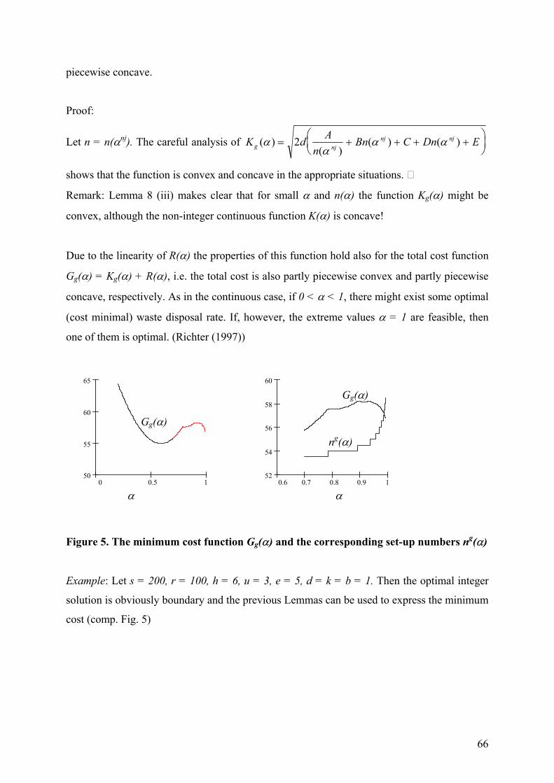
66
piecewise concave.
Proof:
Let n = n(αnj). The careful analysis of K d An
Bn C Dn Eg njnj nj( )
( )( ) ( )α
αα α= + + + +
2
shows that the function is convex and concave in the appropriate situations.
Remark: Lemma 8 (iii) makes clear that for small α and n(α) the function Kg(α) might be
convex, although the non-integer continuous function K(α) is concave!
Due to the linearity of R(α) the properties of this function hold also for the total cost function
Gg(α) = Kg(α) + R(α), i.e. the total cost is also partly piecewise convex and partly piecewise
concave, respectively. As in the continuous case, if 0 < α < 1, there might exist some optimal
(cost minimal) waste disposal rate. If, however, the extreme values α = 1 are feasible, then
one of them is optimal. (Richter (1997))
0 0.5 150
55
60
65
0.6 0.7 0.8 0.9 152
54
56
58
60
Figure 5. The minimum cost function Gg(α) and the corresponding set-up numbers ng(α)
Example: Let s = 200, r = 100, h = 6, u = 3, e = 5, d = k = b = 1. Then the optimal integer
solution is obviously boundary and the previous Lemmas can be used to express the minimum
cost (comp. Fig. 5)
Gg(α)
Gg(α)
ng(α)
αα
67
3.1.3. Conclusion
The EOQ repair and waste disposal model was analyzed. The variable set-up numbers n and
m for production and repair within some collection time interval were supposed to be natural.
First, conditions for some auxiliary fractional program were discussed to have optimal integer
solutions at the boundary of the feasible region. Secondly, these conditions were used to
determine the optimal integer solution and the minimum cost for the repair and waste disposal
model for a wide class of model inputs. Thirdly, it was shown that the minimum cost is a
partly piecewise convex, partly piecewise concave function of the waste disposal rate and the
relative error of optimal boundary solutions is not greater than 2.1 %. Several problems are
subject to further studies as for instance how to determine the optimal integer solution, if the
optimal solution is not boundary, how to include non-linear repair cost and finite
production/repair rates in the integer model.
68
3.2. A Recoverable Item Inventory System
3.2.1. Introduction
Quantitative models for inventory systems with product recovery management provide an
actual generalization of classical EOQ models. The classical EOQ model analyzes one
product inventory systems. The difficulty of recovery system is that a number of authors have
proposed such models. This chapter deals with one of these proposals, we investigate the
model of Teunter (1999).
Teunter in his work has stated that in the proposed model there should be either no more than
one manufacturing batch and no more than one remanufacturing batch in a cycle. A cycle is a
sequence of activities with a fixed number of batches.
The goal of the chapter is to reconsider the Teunter`s model. First the explicit model will be
discussed and a solution is given for this model, because the author has neglected to describe
the explicit model. After solving the problem, we give a counterexample, where the
manufacturing and remanufacturing batches are strictly greater than one. By this
counterexample we show that the Teunter’s graphical proof, that one of the batch numbers
equal to one is not correct. In fact, he proved this property of the batch numbers for the
assumption that only relatively prime (coprime) batch numbers of manufacturing and
remanufacturing are considered, or in other words, for batch numbers with a greatest common
divisors greater than one.
The paper continues the investigations of the proposed model. Now we assume that the
planning horizon, as cycle time, is decision variable.
3.2.2. The model
Teunter has investigated in his model the following activities:
- remanufacturing,
- disposal and
- manufacturing.
69
Let a cycle be the above-mentioned schedule with fixed batch sizes for manufacturing and
remanufacturing. In a planning period there is only one cycle. (This can be proved very easily
by grouping the remanufacturing and manufacturing lots.)
The goal of the decision maker is to minimize the cost for manufacturing and remanufacturing
batch numbers and sizes and for the reuse rate. There are EOQ-oriented setup and holding
costs for remanufacturing and manufacturing, linear production and remanufacturing costs,
linear disposal cost and holding cost for non-serviceable items.
The notations of the model are the following:
System parameters:
- r return rate (0≤r≤1),
- λ rate of demand.
Cost parameters:
- Km setup cost for manufacturing,
- Kr setup cost for remanufacturing,
- hm holding cost for manufactured items,
- hr holding cost for remanufactured items,
- hn holding cost for non-serviceable items,
- cm manufacturing cost,
- cr remanufacturing cost,
- cd cost for disposing one non-serviceable item.
Let us assume that cm + cd > cr, i.e. the unit manufacturing and disposal costs are strictly
greater than the cost of remanufacturing. If the material flow of this model is studied, then it
cen be seen that the disposed items must be newly manufactured. For this reason these two
costs must be summarized. If remanufacturing is economical, then the unit remanufacturing
costs are lower than that of manufacturing and disposal.
Decision variables:
- Qm batch size for manufacturing,
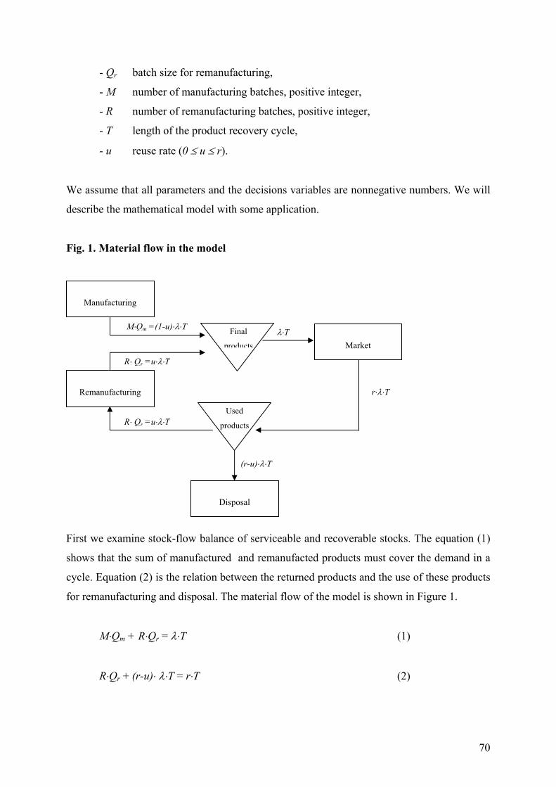
70
- Qr batch size for remanufacturing,
- M number of manufacturing batches, positive integer,
- R number of remanufacturing batches, positive integer,
- T length of the product recovery cycle,
- u reuse rate (0 ≤ u ≤ r).
We assume that all parameters and the decisions variables are nonnegative numbers. We will
describe the mathematical model with some application.
Fig. 1. Material flow in the model
First we examine stock-flow balance of serviceable and recoverable stocks. The equation (1)
shows that the sum of manufactured and remanufacted products must cover the demand in a
cycle. Equation (2) is the relation between the returned products and the use of these products
for remanufacturing and disposal. The material flow of the model is shown in Figure 1.
M⋅Qm + R⋅Qr = λ⋅T (1)
R⋅Qr + (r-u)⋅ λ⋅T = r⋅T (2)
Market
Disposal
Remanufacturing
Used
products
Final
products
M⋅Qm =(1-u)⋅λ⋅T
R⋅ Qr =u⋅λ⋅T
R⋅ Qr =u⋅λ⋅T
λ⋅T
r⋅λ⋅T
(r-u)⋅λ⋅T
Manufacturing
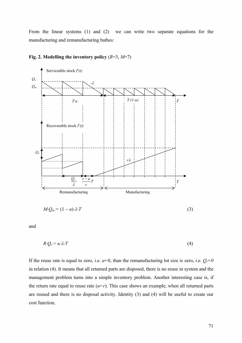
71
From the linear systems (1) and (2) we can write two separate equations for the
manufacturing and remanufacturing bathes:
Fig. 2. Modelling the inventory policy (R=3, M=7)
M⋅Qm = (1 − u)⋅λ⋅T (3)
and
R⋅Qr = u⋅λ⋅T (4)
If the reuse rate is equal to zero, i.e. u=0, than the remanufacturing lot size is zero, i.e. Qr=0
in relation (4). It means that all returned parts are disposed, there is no reuse in system and the
management problem turns into a simple inventory problem. Another interesting case is, if
the return rate equal to reuse rate (u=r). This case shows an example, when all returned parts
are reused and there is no disposal activity. Identity (3) and (4) will be useful to create our
cost function.
Recoverable stock Ir(t)
Serviceable stock Is(t)
T·u
Remanufacturing Manufacturing
Qr
rλ
Tr
ur −λ
rQ
T
-λ Qr
Qm
T·(1-u)
T
72
Now we construct the total cost function. We make it in two steps. In the first step we
investigate the inventory holding cost function H(Qm,Qr,T,M,R,u) for serviceable and non-
serviceable parts.In the second step we describe the linear costs L(Qm,Qr,T,M,R,u) of
manufacturing, remanufacturing, and disposal.
Let us now calculate the inventory holding costs H(Qm,Qr,T,M,R,u). The inventory holding
policy is shown in Figure 2. This policy is a predetermined policy and we look for the optimal
parameters (Qm,Qr,T,M,R,u) of this strategy. Let us assume that the inventory level functions
for a known strategy are function Is(t) for serviceable stock and function Ir(t) for recoverable
stock, 0≤t≤T. The inventory holding costs are the area below this functions, i.e.
( ) ∫∫∫ ⋅+⋅+⋅=⋅
⋅ Tr
n
T
uT
sm
uTs
rrm dttIhdttIhdttIhuRMQQH00
)()()(,,,, .
Now we use the property of the inventory policy that the sum of serviceable and recovarable
products is a monotone decreasing, linear and continuous function of time in the
remanufacturing cycle. So the inventory cycle can be divided into two subcycles.
(1) the demand is satisfied from remanufacturing, and the recoverable stock is positive.
The length of this interval is equal to λ
rQuT −⋅ .
(2) The demand is satisfied from the last remanufacturing batch and from manufacturing,
and the stock level of recoverable items are monotone nondecreasing. A
remanufacturing batch is used in an interval length of λ
rQ . The length of this subcycle
is ( )λ
rQuT +−⋅ 1 .
So the inventory holding cost function can be expressed with the help of the cycles, as
( )
( ) [ ] ∫∫∫∫∫−⋅
−⋅
⋅
⋅
−⋅
−⋅
+++++−
=
T
quT
rn
quT
rsn
T
uT
sm
uT
quT
sr
quT
snr
rm
r
r
r
r
dttIhdttItIhdttIhdttIhdttIhh
uRMQQH
λ
λ
λ
λ
)()()()()()(
,,,,
00
.
73
We must now calculate the five integrals. The first integral consists of R-1 pieces
remanufacturing batches. The costs are ( ) ( ) ( )λ
λ
21)(
2
0
rnr
quT
snr
QhhRdttIhh
r
⋅−⋅−=⋅− ∫−⋅
. The
second integral is only a remanufacturing batch λ
λ
2)(
2r
r
uT
quT
sr
QhdttIh
r
⋅=⋅ ∫⋅
−⋅
. The third value is
the cost of inventory holding of manufactured products, which consists of M batches
λ2)(
2m
m
T
uT
sm
QhMdttIh ⋅⋅=⋅ ∫
⋅
. The computation of the fourth integral is a little bit complicated.
We have pointed out that the sum of the inventory levels Is(t)+Ir(t) is a monotone decreasing
linear function. The tangent of this linear function is (1-r)⋅λ. In point of time λ
rQuT −⋅ this
function has a value of Qr. With this assumption the value of the integral is
[ ] ( )
−⋅⋅
−⋅⋅⋅−+⋅=+⋅ ∫
−⋅
λλλλ
rrrn
quT
rsn
QuT
QuTrQhdttItIh
r
21)()(
0
. The fifth, last
integral is 21
2)(
+⋅⋅−
⋅⋅⋅=⋅ ∫−⋅
λλ
λ
rn
T
quT
rn
QuTr
rrhdttIhr
.
Summing up the integrals and with elementary calculations, we have the following expression
for the inventory holding costs:
( )
+
−⋅⋅⋅+⋅⋅+⋅⋅= R
rrR
Qh
QhM
QhRuRMTQQH r
nm
mr
rrm1
222,,,,, 2
222
λλλ.
In this expression we have applied from equation (4) that λ
rQRuT
⋅=⋅ .
The linear costs of manufacturing, remanufacturing, and disposal can be calculated very
easily:
L(Qm,Qr,T,M,R,u) = cm⋅M⋅Qm + cr⋅R⋅Qr + cd⋅λ⋅T⋅(r-u) = ( ) ( )[ ]rcccccuT dmdmr ⋅++−−⋅⋅⋅ λ
74
Now we can formulate the average cost function Ca(Qm,,Qr,T,M,R,u) summing up the total
inventory holding costs (setup and inventory holding costs) and the linear manufacturing,
remanufacturing, and disposal costs, and divided with the length of the cycle:
( )
( ) ( )rcccccuT
Rr
rRQ
hQ
hMKMQ
hRKR
uRMTQQC
dmdmr
rn
mmm
rrr
rma
⋅+⋅+−−⋅⋅+
+
+
−⋅⋅⋅+⋅⋅+⋅+⋅⋅+⋅
=
=
λλ
λλλ1
222
,,,,,
2222
This way we have constructed a non-linear mixed-integer mathematical programming
problem:
( )
>≥≥≤≤
⋅⋅=⋅⋅⋅−=⋅
→
integers positive,,0,0,00
)1(such that
min,,,,
RMTQQru
TuQRTuQM
uRMTQQC
rm
r
m
rma
λλ
(P)
Before solving problem (P) we will show that
In the next section we will solve the problem for the relevant variables.
3.2.3. Solutions of the model
In this section we solve proble (P) in two different way. The difference is the order of
eliminating the continuous variables from the cost function using equations (3) and (4). The
first method offers to eliminate the integer variables R and M, in order to express the
manufacturing and remanufacturing lot sizes. Second method suggests elimination the lot
sizes in order to investigate an integer programming problem. Let us follow this two ways.
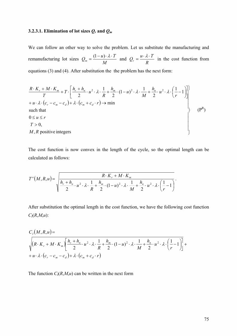
75
3.2.3.1. Elimination of lot sizes Qr and Qm
We can follow an other way to solve the problem. Let us substitute the manufacturing and
remanufacturing lot sizes M
TuQm⋅⋅−
=λ)1( and
RTuQr⋅⋅
=λ in the cost function from
equations (3) and (4). After substitution the the problem has the next form:
( ) ( )
>≤≤
→⋅+⋅+−−⋅⋅+
−⋅⋅⋅+⋅⋅−⋅+⋅⋅⋅
+⋅+
⋅+⋅
integers positive,,0
0such that
min
112
1)1(2
12
222
RMT
ru
rcccccur
uhM
uhR
uhhTT
KMKR
dmdmr
nmnrmr
λλ
λλλ
(PR)
The cost function is now convex in the length of the cycle, so the optimal length can be
calculated as follows:
( )
−⋅⋅⋅+⋅⋅−⋅+⋅⋅⋅
+⋅+⋅
=11
21)1(
21
2
,,222
ru
hM
uh
Ru
hhKMKR
uRMTnmnr
mro
λλλ.
After substitution the optimal length in the cost function, we have the following cost function
CI(R,M,u):
( )
( )
( ) ( )rcccccur
uh
Mu
hR
uhh
KMKR
uRMC
dmdmr
nmnrmr
I
⋅+⋅+−−⋅⋅+
+
−⋅⋅⋅+⋅⋅−⋅+⋅⋅⋅
+⋅+⋅
=
λλ
λλλ 112
1)1(2
12
,,
222
The function CI(R,M,u) can be written in the next form
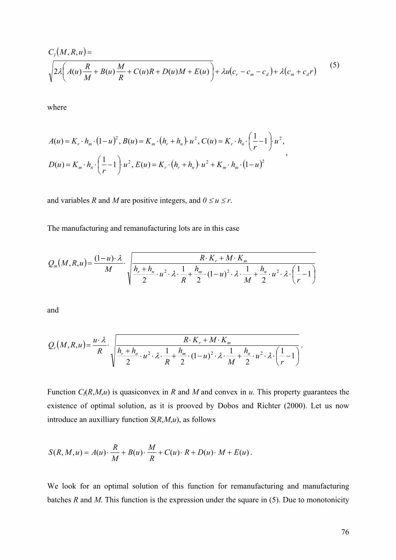
76
( )
( ) ( )rcccccuuEMuDRuCRMuB
MRuA
uRMC
dmdmr
I
++−−+
++++
=
λλλ )()()()()(2
,, (5)
where
( ) ( )
( ) ( )222
222
1)(,11)(
,11)(,)(,1)(
uhKuhhKuEur
hKuD
ur
hKuCuhhKuBuhKuA
mmnrrnm
nrnrmmr
−⋅⋅+⋅+⋅=⋅
−⋅⋅=
⋅
−⋅⋅=⋅+⋅=−⋅⋅=
,
and variables R and M are positive integers, and 0 ≤ u ≤ r.
The manufacturing and remanufacturing lots are in this case
( )
−⋅⋅⋅+⋅⋅−⋅+⋅⋅⋅
+⋅+⋅
⋅⋅−
=11
21)1(
21
2
)1(,,222
ruh
Muh
Ruhh
KMKRMuuRMQ
nmnr
mrm
λλλ
λ
and
( )
−⋅⋅⋅+⋅⋅−⋅+⋅⋅⋅
+⋅+⋅
⋅⋅
=11
21)1(
21
2
,,222
ruh
Muh
Ruhh
KMKRR
uuRMQnmnr
mrr
λλλ
λ .
Function CI(R,M,u) is quasiconvex in R and M and convex in u. This property guarantees the
existence of optimal solution, as it is prooved by Dobos and Richter (2000). Let us now
introduce an auxilliary function S(R,M,u), as follows
)()()()()(),,( uEMuDRuCRMuB
MRuAuMRS +⋅+⋅+⋅+⋅= .
We look for an optimal solution of this function for remanufacturing and manufacturing
batches R and M. This function is the expression under the square in (5). Due to monotonicity
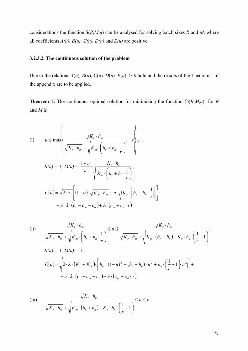
77
considerations the function S(R,M,u) can be analysed for solving batch sizes R and M, where
all coefficients A(u), B(u), C(u), D(u) and E(u) are positive.
3.2.3.2. The continuous solution of the problem
Due to the relations A(u), B(u), C(u), D(u), E(u) > 0 hold and the results of the Theorem 1 of
the appendix are to be applied.
Theorem 1: The continuous optimal solution for minimizing the function CI(R,M,u) for R
and M is
(i)
⋅+⋅+⋅
⋅≤ r
rhhKhK
hKu
nrmmr
mr ,1
max ,
R(u) = 1, M(u) =
⋅+⋅
⋅⋅
−
rhhK
hKu
u
nrm
mr
11 ,
( ) ( )
( ) ( )rcccccu
rhhKuhKuuC
dmdmr
nrrmm
⋅+⋅+−−⋅⋅+
+
⋅+⋅⋅+⋅⋅−⋅⋅=
λλ
λ 112
(ii) ( )
−⋅⋅−+⋅+⋅
⋅≤≤
⋅+⋅+⋅
⋅
111r
hKhhKhK
hKu
rhhKhK
hK
nrnrmmr
mr
nrmmr
mr ,
R(u) = 1, M(u) = 1,
( ) ( )
( ) ( )rcccccu
ur
huhhuhKKuC
dmdmr
nnrmmr
⋅+⋅+−−⋅⋅+
+
⋅
−⋅+⋅++−⋅⋅+⋅⋅=
λλ
λ 222 11)()1(2
(iii) ( )
ru
rhKhhKhK
hK
nrnrmmr
mr ≤≤
−⋅⋅−+⋅+⋅
⋅
11,
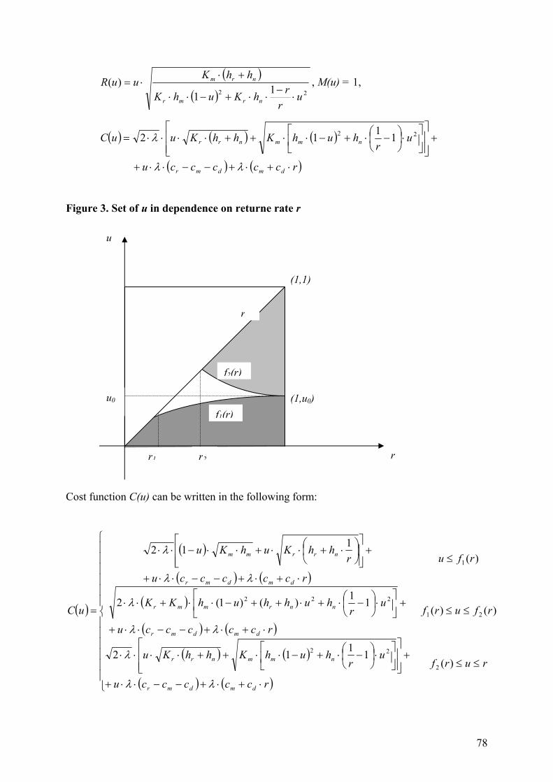
78
( )( ) 22 11
)(u
rrhKuhK
hhKuuR
nrmr
nrm
⋅−
⋅⋅+−⋅⋅
+⋅⋅= , M(u) = 1,
( ) ( ) ( )
( ) ( )rcccccu
ur
huhKhhKuuC
dmdmr
nmmnrr
⋅+⋅+−−⋅⋅+
+
⋅
−⋅+−⋅⋅++⋅⋅⋅⋅=
λλ
λ 22 1112
Figure 3. Set of u in dependence on returne rate r
Cost function C(u) can be written in the following form:
( )
( )
( ) ( )
( )
( ) ( )
( ) ( )
( ) ( )
≤≤
⋅+⋅+−−⋅⋅+
+
⋅
−⋅+−⋅⋅++⋅⋅⋅⋅
≤≤
⋅+⋅+−−⋅⋅+
+
⋅
−⋅+⋅++−⋅⋅+⋅⋅
≤
⋅+⋅+−−⋅⋅+
+
⋅+⋅⋅+⋅⋅−⋅⋅
=
rurf
rcccccu
ur
huhKhhKu
rfurf
rcccccu
ur
huhhuhKK
rfu
rcccccu
rhhKuhKu
uC
dmdmr
nmmnrr
dmdmr
nnrmmr
dmdmr
nrrmm
)(1112
)()(11)()1(2
)(112
2
22
21
222
1
λλ
λ
λλ
λ
λλ
λ
(1,1)
(1,u0)
r1
u
r
f1(r)
f2(r)
r
r2
u0
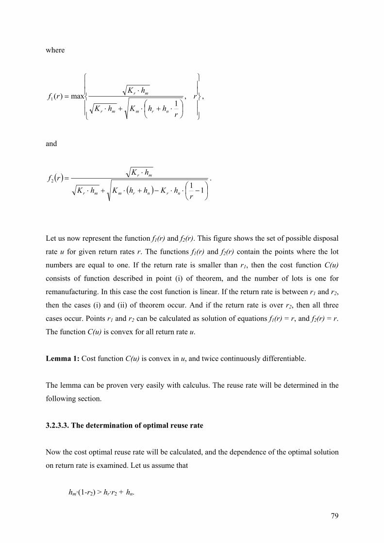
79
where
⋅+⋅+⋅
⋅= r
rhhKhK
hKrf
nrmmr
mr ,1
max)(1 ,
and
( )( )
−⋅⋅−+⋅+⋅
⋅=
112
rhKhhKhK
hKrf
nrnrmmr
mr .
Let us now represent the function f1(r) and f2(r). This figure shows the set of possible disposal
rate u for given return rates r. The functions f1(r) and f2(r) contain the points where the lot
numbers are equal to one. If the return rate is smaller than r1, then the cost function C(u)
consists of function described in point (i) of theorem, and the number of lots is one for
remanufacturing. In this case the cost function is linear. If the return rate is between r1 and r2,
then the cases (i) and (ii) of theorem occur. And if the return rate is over r2, then all three
cases occur. Points r1 and r2 can be calculated as solution of equations f1(r) = r, and f2(r) = r.
The function C(u) is convex for all return rate u.
Lemma 1: Cost function C(u) is convex in u, and twice continuously differentiable.
The lemma can be proven very easily with calculus. The reuse rate will be determined in the
following section.
3.2.3.3. The determination of optimal reuse rate
Now the cost optimal reuse rate will be calculated, and the dependence of the optimal solution
on return rate is examined. Let us assume that
hm·(1-r2) > hr·r2 + hn.
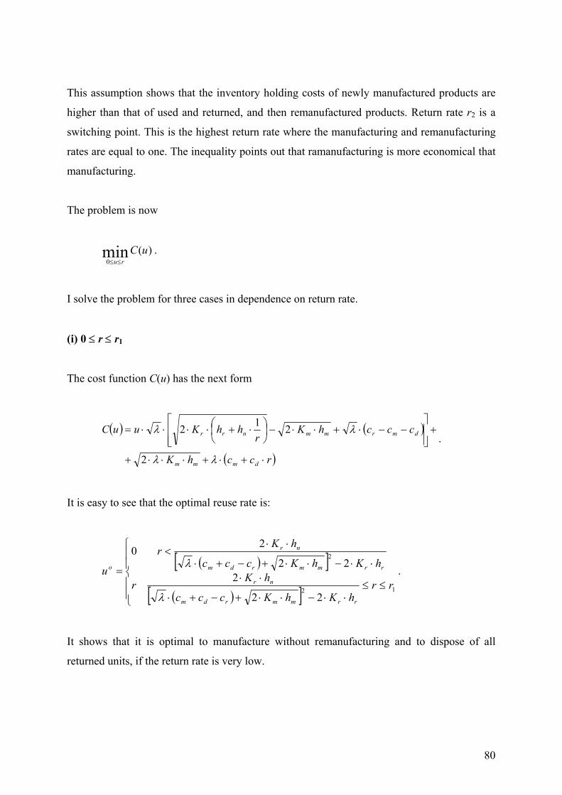
80
This assumption shows that the inventory holding costs of newly manufactured products are
higher than that of used and returned, and then remanufactured products. Return rate r2 is a
switching point. This is the highest return rate where the manufacturing and remanufacturing
rates are equal to one. The inequality points out that ramanufacturing is more economical that
manufacturing.
The problem is now
)(min0
uCru≤≤
.
I solve the problem for three cases in dependence on return rate.
(i) 0 ≤ r ≤ r1
The cost function C(u) has the next form
( ) ( )
( )rcchK
ccchKr
hhKuuC
dmmm
dmrmmnrr
⋅+⋅+⋅⋅⋅+
+
−−⋅+⋅⋅−
⋅+⋅⋅⋅⋅=
λλ
λλ
2
212.
It is easy to see that the optimal reuse rate is:
( )[ ]
( )[ ]
≤≤⋅⋅−⋅⋅+−+⋅
⋅⋅⋅⋅−⋅⋅+−+⋅
⋅⋅<
=12
2
22
222
20
rrhKhKccc
hKr
hKhKccc
hKr
u
rrmmrdm
nr
rrmmrdm
nr
o
λ
λ.
It shows that it is optimal to manufacture without remanufacturing and to dispose of all
returned units, if the return rate is very low.
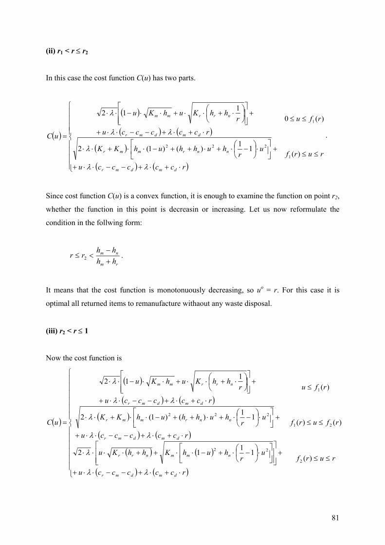
81
(ii) r1 < r ≤ r2
In this case the cost function C(u) has two parts.
( )
( )
( ) ( )
( )
( ) ( )
≤≤
⋅+⋅+−−⋅⋅+
+
⋅
−⋅+⋅++−⋅⋅+⋅⋅
≤≤
⋅+⋅+−−⋅⋅+
+
⋅+⋅⋅+⋅⋅−⋅⋅
=
rurf
rcccccu
ur
huhhuhKK
rfu
rcccccu
rhhKuhKu
uC
dmdmr
nnrmmr
dmdmr
nrrmm
)(11)()1(2
)(0112
1
222
1
λλ
λ
λλ
λ
.
Since cost function C(u) is a convex function, it is enough to examine the function on point r2,
whether the function in this point is decreasin or increasing. Let us now reformulate the
condition in the follwing form:
rm
nm
hhhh
rr+−
<≤ 2 .
It means that the cost function is monotonuously decreasing, so uo = r. For this case it is
optimal all returned items to remanufacture withaout any waste disposal.
(iii) r2 < r ≤ 1
Now the cost function is
( )
( )
( ) ( )
( )
( ) ( )
( ) ( )
( ) ( )
≤≤
⋅+⋅+−−⋅⋅+
+
⋅
−⋅+−⋅⋅++⋅⋅⋅⋅
≤≤
⋅+⋅+−−⋅⋅+
+
⋅
−⋅+⋅++−⋅⋅+⋅⋅
≤
⋅+⋅+−−⋅⋅+
+
⋅+⋅⋅+⋅⋅−⋅⋅
=
rurf
rcccccu
ur
huhKhhKu
rfurf
rcccccu
ur
huhhuhKK
rfu
rcccccu
rhhKuhKu
uC
dmdmr
nmmnrr
dmdmr
nnrmmr
dmdmr
nrrmm
)(1112
)()(11)()1(2
)(112
2
22
21
222
1
λλ
λ
λλ
λ
λλ
λ
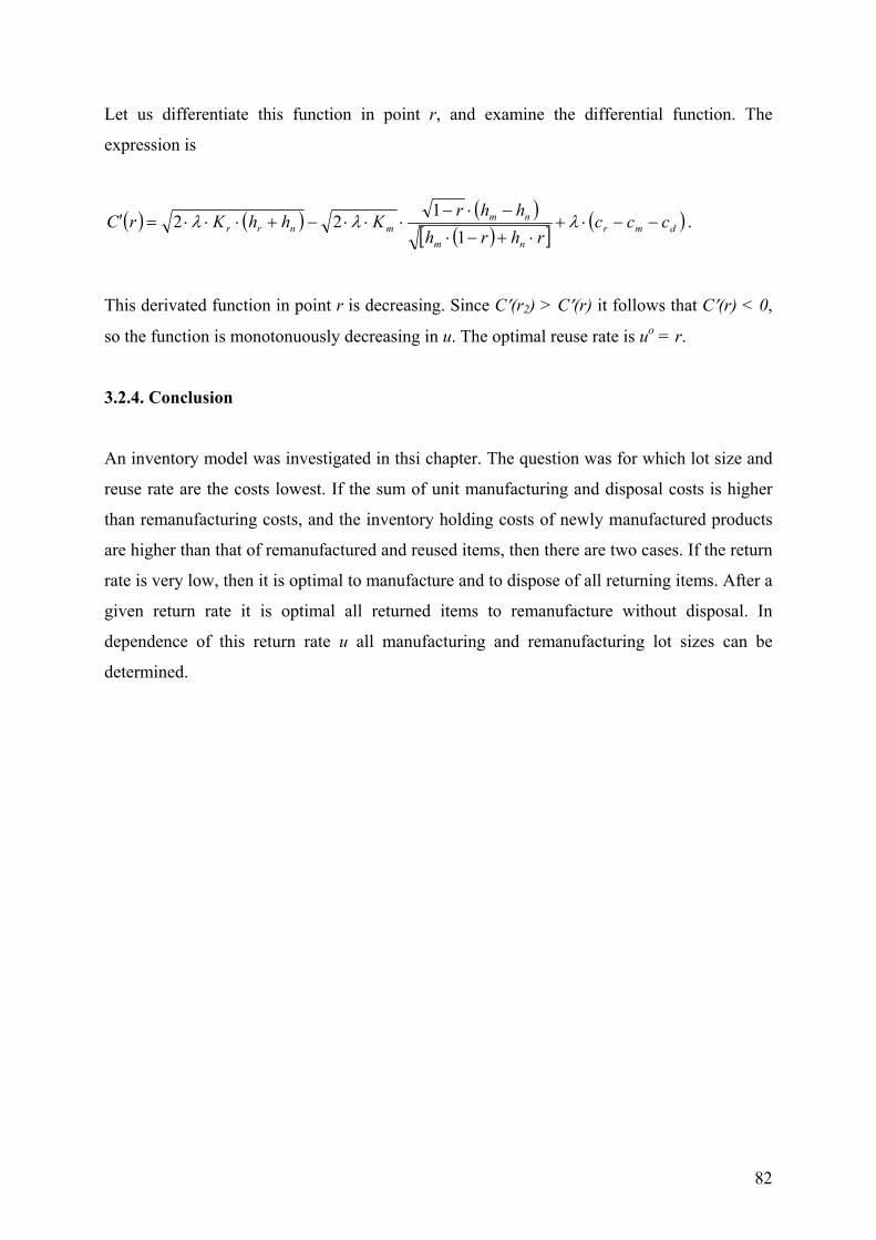
82
Let us differentiate this function in point r, and examine the differential function. The
expression is
( ) ( ) ( )( )[ ]
( )dmrnm
nmmnrr ccc
rhrhhhr
KhhKrC −−⋅+⋅+−⋅
−⋅−⋅⋅⋅−+⋅⋅⋅=′ λλλ
11
22 .
This derivated function in point r is decreasing. Since C′(r2) > C′(r) it follows that C′(r) < 0,
so the function is monotonuously decreasing in u. The optimal reuse rate is uo = r.
3.2.4. Conclusion
An inventory model was investigated in thsi chapter. The question was for which lot size and
reuse rate are the costs lowest. If the sum of unit manufacturing and disposal costs is higher
than remanufacturing costs, and the inventory holding costs of newly manufactured products
are higher than that of remanufactured and reused items, then there are two cases. If the return
rate is very low, then it is optimal to manufacture and to dispose of all returning items. After a
given return rate it is optimal all returned items to remanufacture without disposal. In
dependence of this return rate u all manufacturing and remanufacturing lot sizes can be
determined.
83
3.3. A production-recycling model with buybacking
3.3.1. Introduction
Classical logistic systems manage the material and related informational flow from raw
material until the final products are delivered to the customer. This means a forward flow.
Reverse logistics manages backward process, i.e. the used and reusable parts and products
return from the customers to the producers. Environmental consciousness forces companies to
initiate such product recovery systems. These way natural resources can be saved for the
future generations, so the firms can contribute to the sustainable development efforts. This
work analyzes a situation where the returned items are recycled and the firm saves with the
recycling the mining of other natural resources.
In this paper a model of the EOQ type is developed and analyzed, in which a producer serves
a stationary product demand occurring at the rate D > 0. This demand is served by producing
or procuring new items as well as by recycling some part 0 ≤ δ ≤ 1 of the used products
coming back to the producer at a constant return rate d = αD, 0≤ α ≤ 1. It is assumed that the
producer is in the situation to buy back all used product to recycle and/or to dispose off them.
The parameters δ and α are called marginal use rate and marginal buyback (return) rate,
respectively. The remaining part of the non-serviceable products (1-δ)d will be disposed off.
(1-δ) is called marginal disposal rate.
First, an analysis of the situation is provided. The inventory stocks for serviceable products
from the production and recycling processes (PRP) and for the non-serviceable items is
determined. On the basis of these results the lot sizes and cycle times for the PRP can be
found which minimize the per time unit total set-up and holding cost. This results in the
explicit determination of a function CI(α,δ) which expresses these minimal costs as function
of the marginal use and buyback rates.
Secondly, if linear waste disposal, production, recycling and buyback costs are introduced, the
problem appears at which δ and α the total set-up, holding and linear costs CI(α,δ)+CN(α,δ) is
minimal. In this formulation the producer makes decision about how much used items buy
back to recycle.
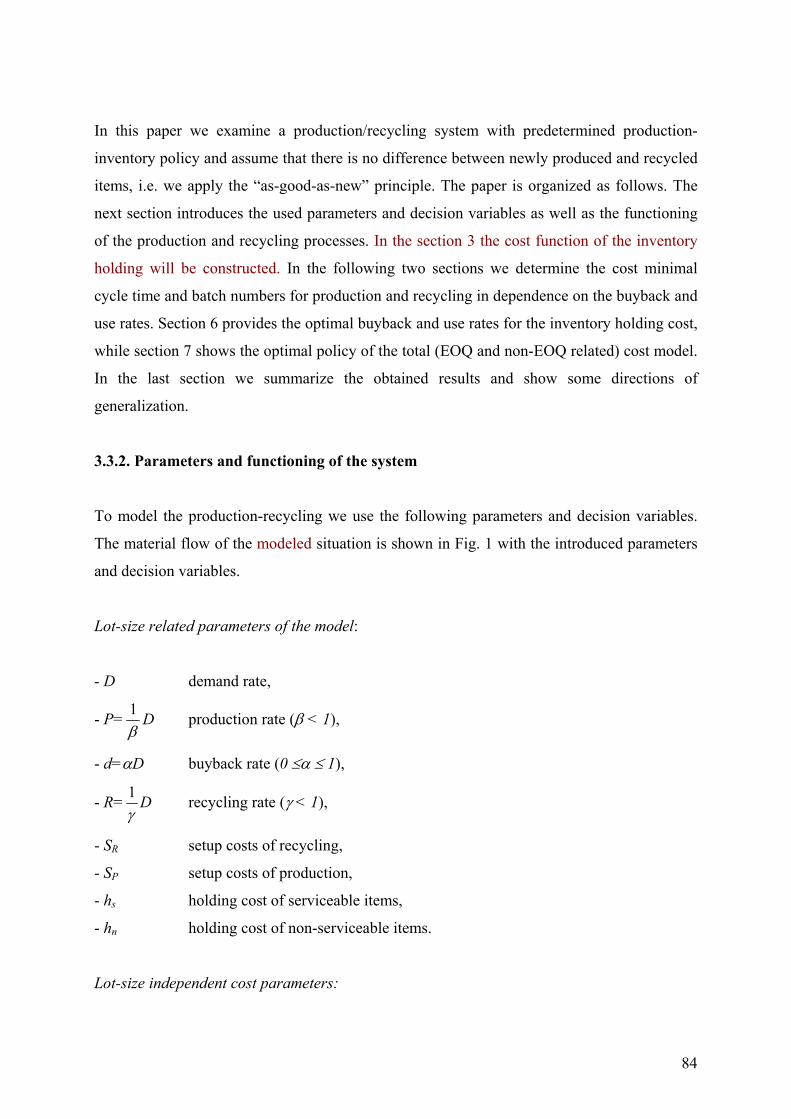
84
In this paper we examine a production/recycling system with predetermined production-
inventory policy and assume that there is no difference between newly produced and recycled
items, i.e. we apply the “as-good-as-new” principle. The paper is organized as follows. The
next section introduces the used parameters and decision variables as well as the functioning
of the production and recycling processes. In the section 3 the cost function of the inventory
holding will be constructed. In the following two sections we determine the cost minimal
cycle time and batch numbers for production and recycling in dependence on the buyback and
use rates. Section 6 provides the optimal buyback and use rates for the inventory holding cost,
while section 7 shows the optimal policy of the total (EOQ and non-EOQ related) cost model.
In the last section we summarize the obtained results and show some directions of
generalization.
3.3.2. Parameters and functioning of the system
To model the production-recycling we use the following parameters and decision variables.
The material flow of the modeled situation is shown in Fig. 1 with the introduced parameters
and decision variables.
Lot-size related parameters of the model:
- D demand rate,
- P=β1 D production rate (β < 1),
- d=αD buyback rate (0 ≤α ≤ 1),
- R=γ1 D recycling rate (γ < 1),
- SR setup costs of recycling,
- SP setup costs of production,
- hs holding cost of serviceable items,
- hn holding cost of non-serviceable items.
Lot-size independent cost parameters:
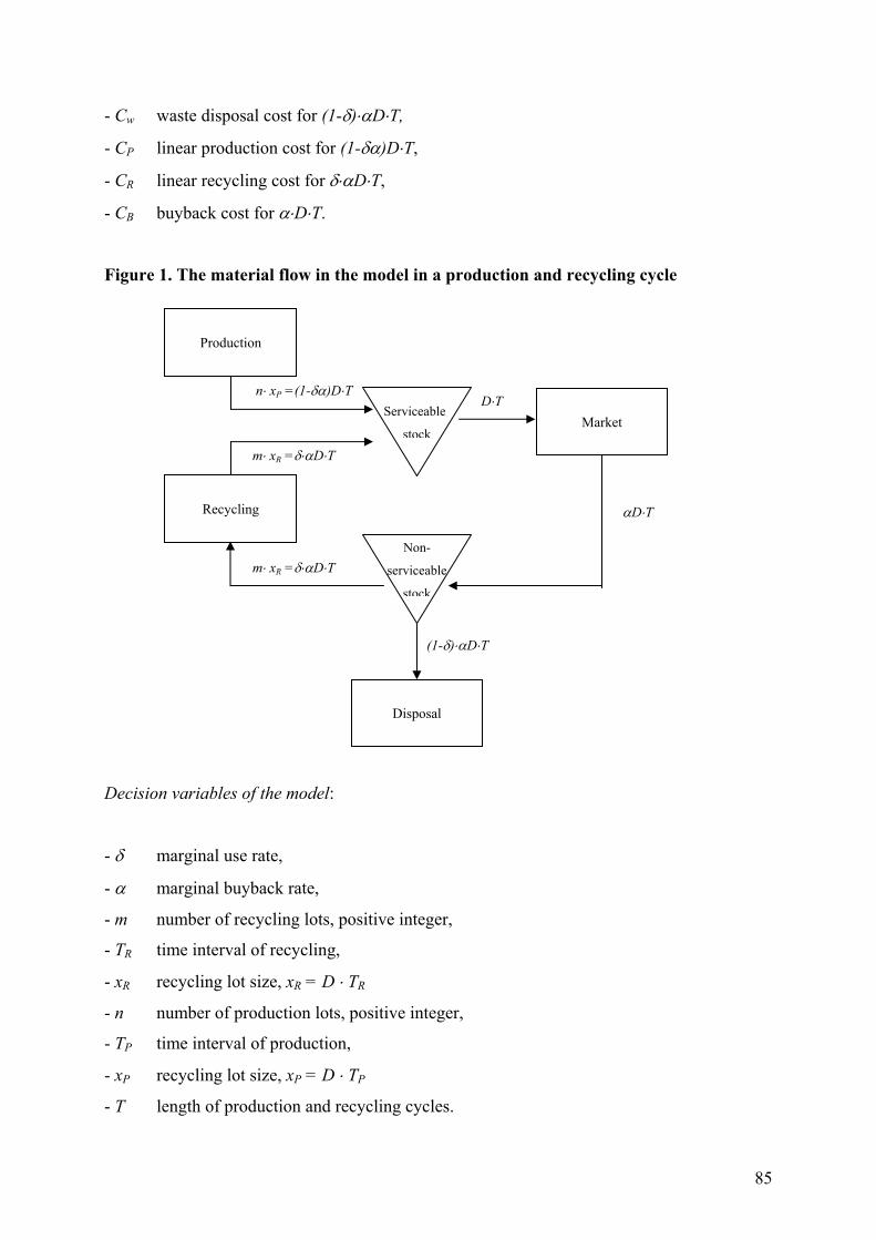
85
- Cw waste disposal cost for (1-δ)⋅αD⋅T,
- CP linear production cost for (1-δα)D⋅T,
- CR linear recycling cost for δ⋅αD⋅T,
- CB buyback cost for α⋅D⋅T.
Figure 1. The material flow in the model in a production and recycling cycle
Decision variables of the model:
- δ marginal use rate,
- α marginal buyback rate,
- m number of recycling lots, positive integer,
- TR time interval of recycling,
- xR recycling lot size, xR = D ⋅ TR
- n number of production lots, positive integer,
- TP time interval of production,
- xP recycling lot size, xP = D ⋅ TP
- T length of production and recycling cycles.
Market
Disposal
Recycling
Non-
serviceable
stock
Serviceable
stock
n⋅ xP =(1-δα)D⋅T
m⋅ xR =δ⋅αD⋅T
m⋅ xR =δ⋅αD⋅T
D⋅T
αD⋅T
(1-δ)⋅αD⋅T
Production
86
Figure 2. Inventory status in the model (m = 3, n = 2)
The demand is satisfied by recycling the non-serviceable products during time period TR , and
stored until the end of this cycle as well as the used products arrive at the rate d =αD < D in
non-serviceable stocking point (compare Fig. 2). Due to the given recycling rate R > D = γR
the process of recycling lasts for some γ ·TR time units. When the recycling process is stopped
the demand can be served by the accumulated stock of recycled products. Parameter of this
figure TR denotes the length of the recycling cycle.
IP
Stock of non-serviceable items
αD
TR
-D
IR
In
αD
-DD
−11
β
Stock of serviceable items
D
−11
γ
D
−γ
α 1
TP
TD
T
T
87
After recycling the producer serves a demand of one product, which appears at a constant rate
D > 0 The producer has to determine how much of new items to produce at a rate P, D = βP
< P. Depending on this information he can found out how long he has to store the excess
production. The time interval in which production and carrying new production is
accomplished is called the production cycle and it is be denoted by TP. The time interval T =
m⋅ TR + n⋅ TP gives the length of the production and recycling cycles.
The process of storing and disposing off non-serviceable goods can be organized in the
following way: the (1-δ)dT units which have to be disposed during some interval T are
disposed during the time disposal interval TD = (1-δ)T just when they arrive. Hence some
stock of non-serviceable items is set up during the collection interval TRC = T - TD = δT.
At the end of the production cycle the inventory stock of non-serviceable products attains its
peak In = [(1-α)m+α(1-γ)]·DTR which is the initial inventory level at the beginning of the
production and recycling cycle. At the end of a recycling period the inventory stock of
serviceable recycled products attains its peak IR = (1-γ)·DTR. The peak of the inventory stock
of newly produced items is IP = (1-β)·DTP.
3.3.3. Determination of the inventory cost
Let hs denote the inventory cost for serviceable items per unit and time unit, and let hn denote
the same cost for non-serviceable items. If the length of the production and recycling cycle T
is given the average inventory cost HP, HR, Hn for the newly produced items, recycled items
and for the non-serviceable items, correspondingly, are as shown in Lemma 1. Let us now
assume that the return rate α and the use rate δ are positive, i.e. there is recycling and the
buyback and use rates are not equal to one, i.e. there is production, as well.
Lemma 1: The average inventory costs are in this model:
( )m
hDThTImH ssRRR11
21
21 222 ⋅−⋅⋅=⋅⋅= δαγ (1)
( )( )n
hDThTInH ssPPP111
21
21 22 ⋅−−⋅⋅=⋅⋅= αδβ (2)
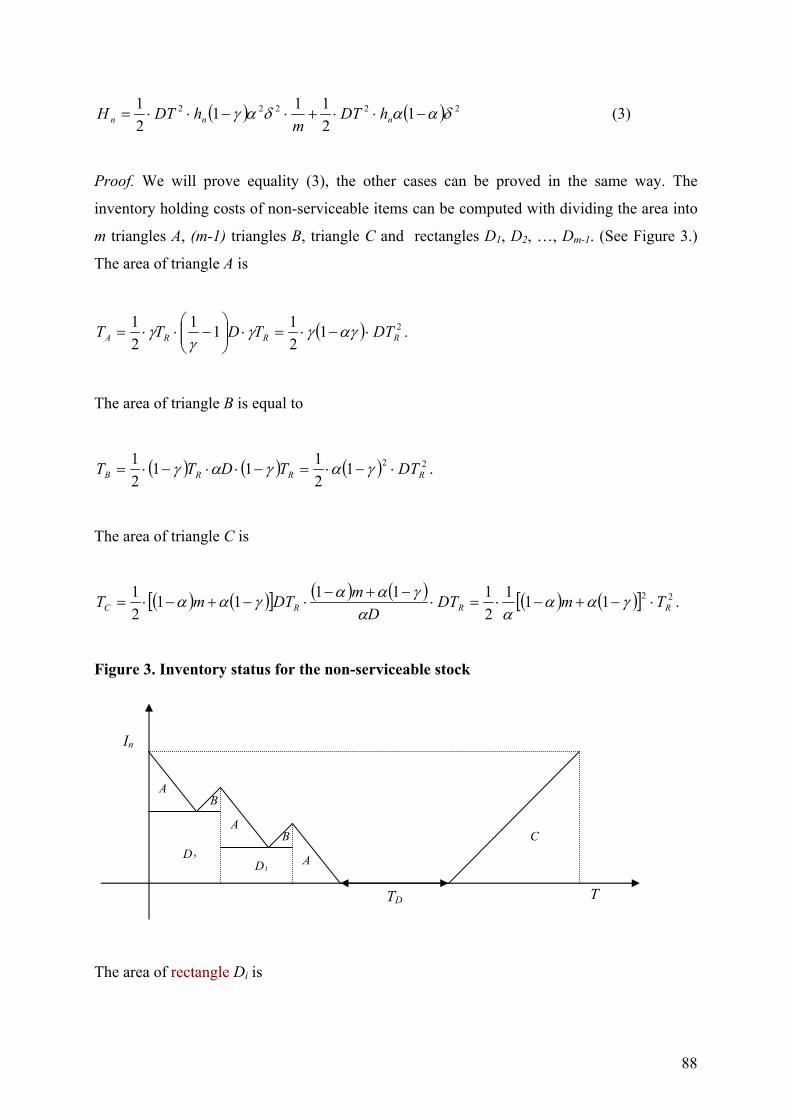
88
( ) ( ) 22222 12111
21 δααδαγ −⋅⋅+⋅−⋅⋅= nnn hDT
mhDTH (3)
Proof. We will prove equality (3), the other cases can be proved in the same way. The
inventory holding costs of non-serviceable items can be computed with dividing the area into
m triangles A, (m-1) triangles B, triangle C and rectangles D1, D2, …, Dm-1. (See Figure 3.)
The area of triangle A is
( ) 212111
21
RRRA DTTDTT ⋅−⋅=⋅
−⋅⋅= αγγγ
γγ .
The area of triangle B is equal to
( ) ( ) ( ) 2212111
21
RRRB DTTDTT ⋅−⋅=−⋅⋅−⋅= γαγαγ .
The area of triangle C is
( ) ( )[ ] ( ) ( ) ( ) ( )[ ] 22111211111
21
RRRC TmDTD
mDTmT ⋅−+−⋅=⋅−+−
⋅−+−⋅= γαααα
γααγαα .
Figure 3. Inventory status for the non-serviceable stock
The area of rectangle Di is
In
TD T
A
A
A
C
B
B D2
D1
89
( ) 21 RiD DTiT α−⋅= .
The total costs are now
( ) ∑−
=
++⋅−+⋅=1
11
m
iiDCBAn TTTmTmH .
After some simple calculation we get the result of (3).
Lemma 2: The total inventory cost per time unit is
HT = =++
THHH nRP ),,,(
21 δαnmVTD ⋅ (4)
with
( )( ) ( )( ) ( ) 2222 111111),,,( δαααδβδαγδα −+⋅−−+⋅−+= nsns hn
hm
hhnmV (5)
Proof. Formulas (4) and (5) are obtained, if the cost and time parameters on the left-hand side
of (4) are substituted by the expressions (1) – (3).
Example 1: Let D = 1,000, hs = 850, hn = 80, β = 2/3, γ = 2/3, m = 1, n = 2, α = 1/2 and δ =
2/3. For this data V(2,1,1/2,2/3) = 0.167hs+ 0.130hn = 106.296 and HT = 296.106000,121
⋅⋅⋅T
53,148.1T hold.
The function ),,,( δαnmV expresses the total inventory cost per time unit and per demand
unit.
3.3.4. Total cost minimization for the cycle time
Let the setup cost S per production and recycling cycle as the sum of setup costs SP and SR for
the production and the recycling, respectively, be given. Then the setup cost per time unit is
90
( ) nSmSnmS PRT ⋅+⋅=, .
The average inventory costs of the model CA(T,m,n,α,δ) can be written in the following form
( )min),,,(
21,),,,,( →⋅+= δαδα nmVTD
TnmSnmTC T
A (6)
Because of the convexity of the cost function in the production and recycling cycle time the
cost optimal cycle time is ( )
),,,(,2),,,(
δαδα
nmVDnmSnmT To
⋅= (7)
and the minimal total setup and inventory cost per time unit is
( ) ),,,(,2),,,(~ δαδα nmVnmSDnmC TA ⋅⋅= . (8)
The optimal recycling and production cycle times are
( )
),,,(,2),,,(
δααδδα
nmVDnmS
mnmT To
R ⋅= , (9)
( )
),,,(,21),,,(
δααδδα
nmVDnmS
nnmT To
P ⋅−
= . (10)
The optimal lot sizes are
( )
),,,(,2),,,(δα
αδδαnmV
nmDSm
nmx ToR = , (11)
( )
),,,(,21),,,(δα
αδδαnmV
nmDSn
nmx ToP
−= . (12)
Example 2: Let as in examples 1 D = 1,000, hs = 850, hn = 80, β = 2/3, γ = 2/3, m = 1, n = 2,
α = 1/2 and δ = 2/3. It is known from Example 1 that V(m,n,α,δ) = 106.296 and HT =
91
53,148.1T hold. Setting SP = 1,960 and SR = 440 the total cost per time unit is according to
formula (6) TT
TCA 1.148,53360,432,
21,2,1, +=
. The optimal length of the production cycle
and recycling cycle is 286.032,
21,2,1 =
T year or 104 days. The minimal cost per time unit
is
1.445,301.148,53360,4232,
21,2,1~
=⋅=
AC .
3.3.5. The optimal number of lots for production and recycling
Now we will minimize the cost function ),,,(~ δαnmCA in order to determine the optimal
number of lots. After some calculation this cost function can be written in the following the
form
( ) ( ) ( ) ( ) ( )
+⋅+⋅+⋅+⋅⋅= δαδαδαδαδαδα ,,,,,2),,,(~ EnDmC
mnB
nmADnmC A (13)
where
( ) ( )( ) ( ) ( )( )( ) ( ) ( ) ( )( ) ( )( ) ( )( )222
22
222
111,
,1,,1,
,1,,11,
αδβδαγδα
δααδαδααδα
δαγδααδβδα
−−+−+=
−=−=
−+=−−=
sPnsR
nPnR
nsPsR
hShhSE
hSDhSC
hhSBhSA
To solve this problem we can introduce a relaxed auxiliary problem (meta-model) (Richter
(1996), Dobos and Richter (2000)):
min),( →++++= EDnCmmnB
nmAnmS , m ≥ 1, n ≥ 1.
Applying the results of Dobos and Richter (2000), the optimal continuous solution for the lots
number (m,n) is
92
Lemma 3: There are three cases of optimal continuous solutions (m(α,δ),n(α,δ)) and
minimum cost expressions CI(α,δ) for the function (13):
(i) A(α,δ) ≥ B(α,δ)+D(α,δ), B(α,δ) ≤ A(α,δ)+C(α,δ)
( ) ( )( ) ( )( )( ) ( )
−+−+−−
=αααγ
βδαδδαδα
1111,1,,, 2
nns
s
P
Roo
hhhh
SSnm
( ) ( ) ( ) ( )( ) ( )[ ]{ }αααγδβαδδα −+−+⋅+−⋅−= 11112, 2nnsRsPI hhhShSDC
(ii) A(α,δ) ≤ B(α,δ)+D(α,δ), B(α,δ) ≤ A(α,δ)+C(α,δ)
( ) ( )( ) ( )1,1,,, =δαδα oo nm
( ) ( ) ( )( ) ( )( ) ( )[ ]2222 11112, δααδαγαδβδα −+−++−−+= nnssPRI hhhhSSDC
(iii) A(α,δ) ≤ B(α,δ)+D(α,δ), B(α,δ) ≥ A(α,δ)+C(α,δ)
( ) ( )( ) ( )( )( )( ) ( )
−+−−
−+⋅⋅= 1,
1111
,,,22 δαααδβ
γαδδαδα
ns
ns
R
Poo
hhhh
SSnm
( ) ( )( ) ( )( ) ( )[ ]{ }22 11112, δαααδβγαδδα −+−−+−+⋅= nsPnsRI hhShhSDC
Note that the expressions for the found optimal lot (batch) numbers are not necessarily
integer! Nevertheless we shall see in the next section that this (immediately practically not
very useful) result will help us to prove that the mixed strategies are dominated by pure ones.
Now we introduce the following functions
( ) ( )( ) ( )( ) ( )[ ]αααγβα
βαδ
−+−++−⋅
−⋅=
111
121
nnsPsR
sR
hhhShS
hS
and
93
( ) ( )( ) ( )( ) ( )αααγβα
βαδ
−⋅−−+⋅+−⋅
−⋅=
111
122
nRnsPsR
sR
hShhShS
hS.
Functions δ1(α) and δ2(α) are such switching points for which the optimal number of lots
(m,n) is equal to one. This is shown in Figure 5. Function δ1(α) separates the cases (i) and (ii)
and δ2(α) the cases (ii) and (iii). To calculate the functions, we have used the conditions in
cases of equality. It is easy to see that δ1(α) ≤ δ2(α). The proof is left to the reader.
Let us now define the possible sets for (α,δ) with the help of functions δ1(α) and δ2(α):
( ) ( ){ }10,10,, 1 ≤≤≤≤≤= δααδδδαI ,
( ) ( ) ( ){ }10,10,, 21 ≤≤≤≤≤≤= δααδδαδδαJ ,
( ) ( ){ }10,10,, 2 ≤≤≤≤≥= δααδδδαK .
The set I is represented by the borders of the possible values of (α,δ), the function δ1(α) and
the points (α1,1) and (1,δ0), where value α1 is the solution of the following equality for α
( )( ) ( )( ) ( )[ ] ( )αδ
αααγβα
β12 111
11 =
−+−++−⋅
−⋅=
nnsPsR
sR
hhhShS
hS
and
( )( ) ( )( )γβ
βδ
−+⋅+−⋅
−⋅=
111
0nsPsR
sR
hhShShS
.
And the set K is represented by the borders of the possible values of (α,δ), the function δ2(α)
and the points (α2,1) and (1,δ0), where value α1 is the solution of the following equality for α
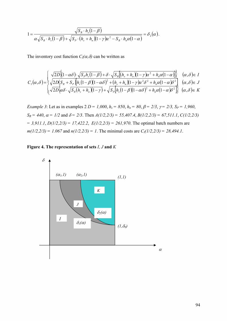
94
( )( ) ( )( ) ( )
( )αδαααγβα
β22 111
11 =
−⋅−−+⋅+−⋅
−⋅=
nRnsPsR
sR
hShhShS
hS.
The inventory cost function CI(α,δ) can be written as
( )( ) ( ) ( )( ) ( )[ ]{ } ( )
( ) ( )( ) ( )( ) ( )[ ] ( )( )( ) ( )( ) ( )[ ]{ } ( )
∈−+−−+−+⋅
∈−+−++−−+
∈−+−+⋅+−⋅−
=
KhhShhSD
JhhhhSSD
IhhhShSD
C
nsPnsR
nnssPR
nnsRsP
I
δαδαααδβγαδ
δαδααδαγαδβ
δααααγδβαδ
δα
,11112
,11112
,11112
,22
2222
2
Example 3: Let as in examples 2 D = 1,000, hs = 850, hn = 80, β = 2/3, γ = 2/3, SP = 1,960,
SR = 440, α = 1/2 and δ = 2/3. Then A(1/2,2/3) = 55,407.4, B(1/2,2/3) = 67,511.1, C(1/2,2/3)
= 3,911.1, D(1/2,2/3) = 17,422.2, E(1/2,2/3) = 261,970. The optimal batch numbers are
m(1/2,2/3) = 1.067 and n(1/2,2/3) = 1. The minimal costs are CI(1/2,2/3) = 28,494.1.
Figure 4. The representation of sets I, J and K
(1,1)
(1,δ0)
(α2,1) (α1,1)
δ
α
I
J
K
δ1(α)
δ2(α)
95
3.3.6. Minimizing the inventory holding costs for the buyback and use rates
Before minimizing the inventory holding costs CI(α,δ) we will prove a simple lemma.
Lemma 3: Let values a, b, c and d be positive. Then the following equality holds
( )( ) bdacdcba +≥++ .
Proof. Let both sides of the inequality raise to the second power. Then
( )( ) abcdbdacdcba 2++≥++
and after simplifying
abcdbcad 2≥+
and this inequality holds for all positive a, b, c and d, because ( ) 02≥− bcad .
Let us apply this result to the strategy with one-one lots:
( ) ( )( ) ( ) ( )[ ] JhhhSSDC nssRPI ∈−+−+−−⋅+= ),(,11112),( 2222 δαδααδαγαδβδα .
Let now
( )( )( ) ( ) 222
2
11
11
22
δααδαγ
αδβ
−+−=
−−=
==
ns
s
R
P
hhd
hc
DSbDSa
Using the result of lemma 3 we have the following inequalities
96
( )( ) ( ) ( )[ ]( ) ( ) ( )( )γαδβαδ
δααδαγαδβδα
−+⋅+−⋅−≥
≥−+−⋅+−−⋅≥
12121
112112),( 2222
nsRsP
nsRsPI
hhDShDS
hhDShDSC
The last inequality holds because we have reduced the costs with the expression
( ) 21 δαα −nh . With this method it can be shown that over sets I and K
( ) ( ) ( )( )γαδβαδδα −+⋅+−⋅−≥ 12121),( nsRsPI hhDShDSC
The last expression is a convex linear combination of the pure strategies, i.e. the recycling and
production. The weights are the possible products of marginal use and buyback rates αδ
which is non-negative and not greater than one. This cost expression is always greater than
the smaller of the costs of pure strategies:
( ) ( ) ( )( )( ) ( )( ){ }γβ
γαδβαδ
−+⋅−⋅≥
≥−+⋅+−⋅−
12;12min
12121
nsRsP
nsRsP
hhDShDS
hhDShDS
By this last inequality a proof is given for the
Theorem 1: The optimal inventory holding strategy in this production-recycling model is a
pure strategy: either to produce to meet the demand (αo = δo = 0) or to buy back and to
recycle all used product without production (αo = δo = 1).
Example 5. Let D=1,000, β = γ = 2/3, SP =1960, SRR =440, hs = 850 and hn = 80. Then the
inventory holding costs of recycling is 16,516.7 and that of production 33,326.7. It is
economical to recycle with buyback of all used items.
Example 6. Let D=1,000, β =2/5 γ = 2/3, SP =360, SRR =440, hs = 85 and hn = 80. Then the
inventory holding costs of production is 6,059.7 and that of recycling 6,957.01. It is more
effective to produce and not to recycle.
97
7. Minimizing the total lot-size related and lot-size independent costs
In this section we minimize the sum of the EOQ-related and EOQ independent costs. The cost
function is in this case
( ) ( )δαδαδα ,),(, NIT CCC +=
where function ( ) ( ) ( ) DCDCDCDCC BPRWN αδαδααδδα ⋅+−⋅+⋅+−⋅= 11, is the sum of
the linear waste disposal, recycling, production and buyback costs.
The problem to be solved has the form
min),( →αδTC
subject to
[ ] [ ]1,0,1,0 ∈∈ αδ .
In the last section we have seen that
( ) ( ) ( )( )γαδβαδδα −+⋅+−⋅−≥ 12121),( nsRsPI hhDShDSC
i.e. the inventory holding costs are not greater than the convex linear combination of the pure
production and recycling strategies. The non-EOQ related costs can be approximated in the
following way
( ) ( ) ( )RBPN CCDCDC +⋅+⋅−≥ δαδαδα 1, .
To get this inequality, we have reduced the lot-size independent costs with the waste disposal
costs ( ) DCW αδ−⋅ 1 and with costs of bought back but not recycled items ( ) DCB αδ−⋅ 1 .
Using these two approximations we can give a lower bound of the total cost function
98
( ) ( ){ } ( )( ) ( ){ }RBnsRPsPT CCDhhDSCDhDSC +⋅+−+⋅+⋅+−⋅−≥ γαδβαδδα 12121),( .
The right-hand expression is again a convex linear combination of the pure strategies, so
( ) ( ){ } ( )( ) ( ){ }( ) ( )( ) ( ){ }RBnsRPsP
RBnsRPsP
CCDhhDSCDhDS
CCDhhDSCDhDS
+⋅+−+⋅⋅+−⋅
≥+⋅+−+⋅+⋅+−⋅−
γβ
γαδβαδ
12,12min
12121.
This result proves the next
Theorem 2: The optimal production-recycling strategy for the total cost model is either to
buyback all sold and used items (αo = δo = 1) or to produce new items without buybacking
and recycling (αo = δo = 0).
This result was shown by Richter [10] for another waste disposal model and by Dobos and
Richter [3] for a production/recycling model. In the case of linear waste disposal, production,
recycling and buyback costs and free choice of buyback and recycling rates between 0 and 1
one of the pure strategies to buy back and recycle or to produce is optimal. The optimal pure
strategy can be found by comparing the values ( ) PsP CDhDS ⋅+−⋅ β12 and
( )( ) ( )RBnsR CCDhhDS +⋅+−+⋅ γ12 .
8. Conclusions and further research
In this chapter we have investigated a production-recycling model. By minimizing the
inventory holding costs it was shown that one of the pure strategies (to produce or to recycle
all products) is optimal. A similar proposition can be obtained minimizing the total EOQ and
non-EOQ related costs. A similar result was obtained by Richter (1997) in a waste disposal
model with remanufacturing and by Dobos and Richter (2003) in a production and recycling
model.
Probably these pure strategies are technologically not feasible and some used products will
not return or even more as the sold ones will come back, and some of them will be not
99
recyclable. This kind of generalization of this basic model could be the introduction of an
upper bound on the buyback rate which is strongly smaller than one. In such a case a mixed
strategy would be economical compared to the pure strategy “production”.
An other way to generalize this model is to ask for the quality of the bought back products. In
the proposed model we have assumed that all returned items are serviceable. One can be put a
question: Who must control the quality of the returned items? If the suppliers examine the
quality of the reusable products, then the buyback rate is strongly smaller than one. If the user
makes it, then not all returned items are recyclable, i.e. the use rate is smaller than one. Which
one of the control systems are more cost advantageous in this case?
100
4. Production Planning in Reverse Logistics
4.1. Introduction
Several management problems arise along the reverse material flow. Some important
questions are the collection of used products and materials and organization of this process;
transportation, storage, and stocking of products, as well as introduction of parts and modules
in the production planning process after organization and control of disassembly.
One of the important research and application field is the integration of reuse in the
production planning. There are only a few international publications on this field. Most of
them are German speaking literature. (Inderfurth (1998), Spengler et al. (1997), Rautenstrauch
(1997)) There are some Anglo-Saxon papers on this field. (Ferrer-Whybark (2000), Guide
(2000)) As I know, there are no Hungarian publications that investigate this problem. In this
chapter I do not examine the organization of return processes, i.e. return management.
This chapter consists of following sections. The second section tries to extend production
planning with reuse. It means that I give some insights in the connection of production
planning and recycling planning. I create a model to analyze disassembly planning, which can
be viewed as a “negative” bill of material. The next section presents the integration of reuse in
the MRP production planning and control system. I show a material requirement planning
(MRP) item record, and the planning steps till the use of materials. The fourth section
summarizes the role of recycling in production planning.
4.2. An extension of production planning with reuse
The collection and reuse of used products and materials cause new problems in the production
planning, which necessitates a connection between MRP and recycling planning. Involvement
of recycling in material flow means a new problem in material management.
Production planning and control systems are developed for traditional production processes,
which is not characterized by a cyclical material flow. The role of recycling activities has
increased because of decreasing amount of raw materials and of rise in storage prices, which
101
have economic and ecological causes. Strong social pressure and increasing governmental
regulation make a current problem from reuse.
In this chapter I define recycling as a return of used products from production process and
from outside, in order to reuse of these used products. Internal recycling products are those
products that are not necessary in a following production process, i.e. by-products, or wastes.
External recycling products are those products that are at the end of life and they originate
from the consumer processes. Both internal and external recycling products are reused then in
the production process. The aim of a recycling process is to produce new products from
recycled products or to manufacture reusable parts and modules for further use. The further
not usable parts and materials can be sold in a second hand market or disposed outside.
Material flow extended with recycling processes involves storage of raw materials, semi-
finished products, end-products, and recycling products. Uncertainty of wastes and returned
products in time, quality and quantity, and uncertainty of duration of reuse process make the
recycling planning process uncertain. So the planning becomes a more complex problem, and
there are a number of decision variables in the decision making. The first situation is decision
about disassembly, reuse and use processes. A second relevant decision is on the field of
manufacturing and purchasing, i.e. the substitution between recycled and newly procured
products and materials, as alternative possibility of material supply. From this context it is
clear that an integration of production and recycling planning is necessary.
Recycling planning, as production planning as well, means a strategic and tactical point of
view, and then it has an operative content. This operative content can be divided as an original
production planning and control, quantity planning, time and capacity planning, and
manufacturing planning. Of course, these activities are extended with recycling activities.
Program planning in recycling means a demand forecasting of type, quantity and duration of
recycling products. On the basis of this forecasting the recycling activity can be formed, and
on the basis of forecasted and returned products an active planning can be developed. If this
forecasting is not taken to be account, then this process is defined as passive recycling
planning, because the enterprise reacts only on the known amount of returned recycling
products.
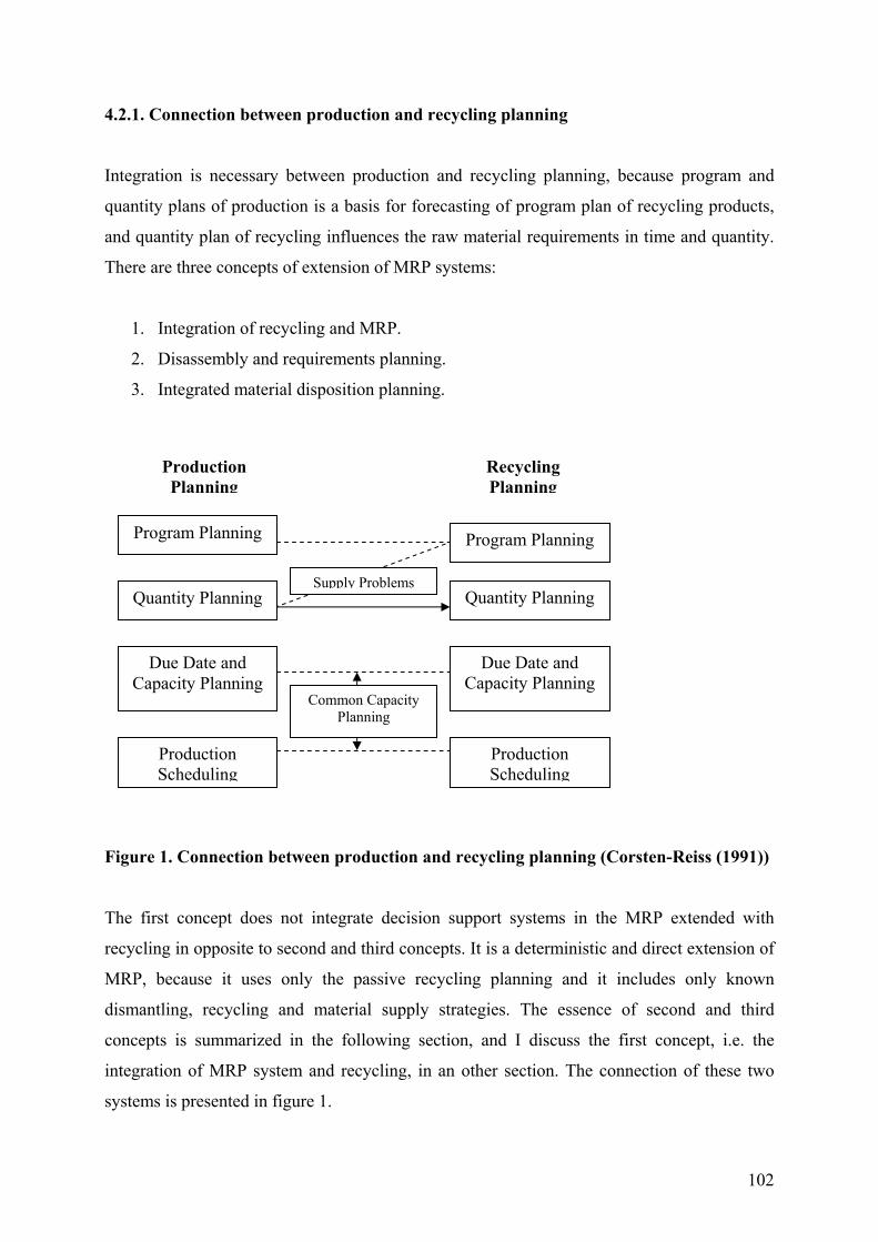
102
4.2.1. Connection between production and recycling planning
Integration is necessary between production and recycling planning, because program and
quantity plans of production is a basis for forecasting of program plan of recycling products,
and quantity plan of recycling influences the raw material requirements in time and quantity.
There are three concepts of extension of MRP systems:
1. Integration of recycling and MRP.
2. Disassembly and requirements planning.
3. Integrated material disposition planning.
Figure 1. Connection between production and recycling planning (Corsten-Reiss (1991))
The first concept does not integrate decision support systems in the MRP extended with
recycling in opposite to second and third concepts. It is a deterministic and direct extension of
MRP, because it uses only the passive recycling planning and it includes only known
dismantling, recycling and material supply strategies. The essence of second and third
concepts is summarized in the following section, and I discuss the first concept, i.e. the
integration of MRP system and recycling, in an other section. The connection of these two
systems is presented in figure 1.
Production Planning
Recycling Planning
Program Planning
Production Scheduling
Production Scheduling
Quantity Planning
Due Date and Capacity Planning
Due Date and Capacity Planning
Quantity PlanningSupply Problems
Common Capacity Planning
Program Planning
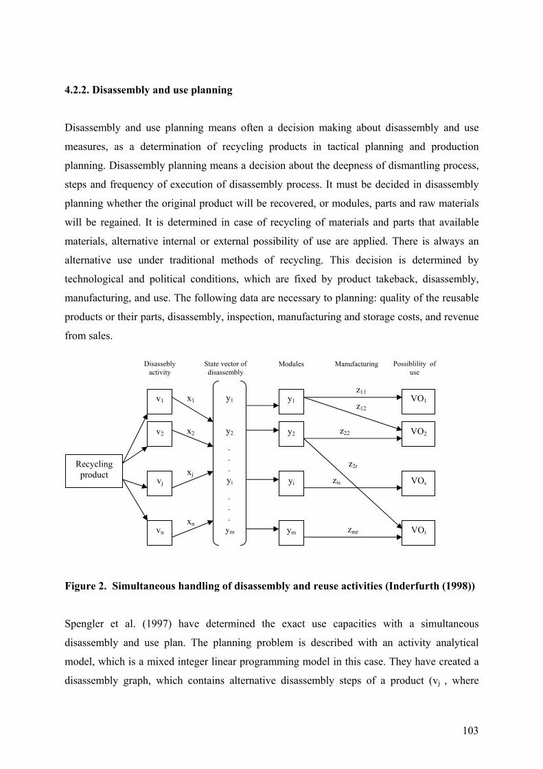
103
4.2.2. Disassembly and use planning
Disassembly and use planning means often a decision making about disassembly and use
measures, as a determination of recycling products in tactical planning and production
planning. Disassembly planning means a decision about the deepness of dismantling process,
steps and frequency of execution of disassembly process. It must be decided in disassembly
planning whether the original product will be recovered, or modules, parts and raw materials
will be regained. It is determined in case of recycling of materials and parts that available
materials, alternative internal or external possibility of use are applied. There is always an
alternative use under traditional methods of recycling. This decision is determined by
technological and political conditions, which are fixed by product takeback, disassembly,
manufacturing, and use. The following data are necessary to planning: quality of the reusable
products or their parts, disassembly, inspection, manufacturing and storage costs, and revenue
from sales.
Figure 2. Simultaneous handling of disassembly and reuse activities (Inderfurth (1998))
Spengler et al. (1997) have determined the exact use capacities with a simultaneous
disassembly and use plan. The planning problem is described with an activity analytical
model, which is a mixed integer linear programming model in this case. They have created a
disassembly graph, which contains alternative disassembly steps of a product (vj , where
Recycling product
z11
z12
z22
z2r
zis
zmr xn
xj
x2
x1
.
.
.
y1
y2
yi
ym
Disassebly activity
State vector of disassembly
Modules Manufacturing Possiblility of use
v1
v2
vj
vn
y1
y2
yi
ym
VO1
VO2
VOs
VOr
.
.
.
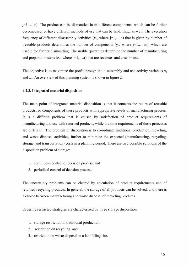
104
j=1,…..n). The product can be dismantled in m different components, which can be further
decomposed, or have different methods of use that can be landfilling, as well. The execution
frequency of different disassembly activities (xj,, where j=1,….n) that is given by number of
treatable products determines the number of components (yji, where j=1,… m), which are
usable for further dismantling. The usable quantities determine the number of manufacturing
and preparation steps (zis, where s=1,….r) that are revenues and costs in use.
The objective is to maximize the profit through the disassembly and use activity variables xj
and zis. An overview of this planning system is shown in figure 2.
4.2.3. Integrated material disposition
The main point of integrated material disposition is that it connects the return of reusable
products, or components of these products with appropriate levels of manufacturing process.
It is a difficult problem that is caused by satisfaction of product requirements of
manufacturing and use with returned products, while the time requirements of these processes
are different. The problem of disposition is to co-ordinate traditional production, recycling,
and waste disposal activities, further to minimize the expected (manufacturing, recycling,
storage, and transportation) costs in a planning period. There are two possible solutions of the
disposition problem of storage:
1. continuous control of decision process, and
2. periodical control of decision process.
The uncertainty problems can be cleared by calculation of product requirements and of
returned recycling products. In general, the storage of all products can be solved, and there is
a choice between manufacturing and waste disposal of recycling products.
Ordering restricted strategies are characterized by three storage disposition:
1. storage restriction in traditional production,
2. restriction on recycling, and
3. restriction on waste disposal in a landfilling site.
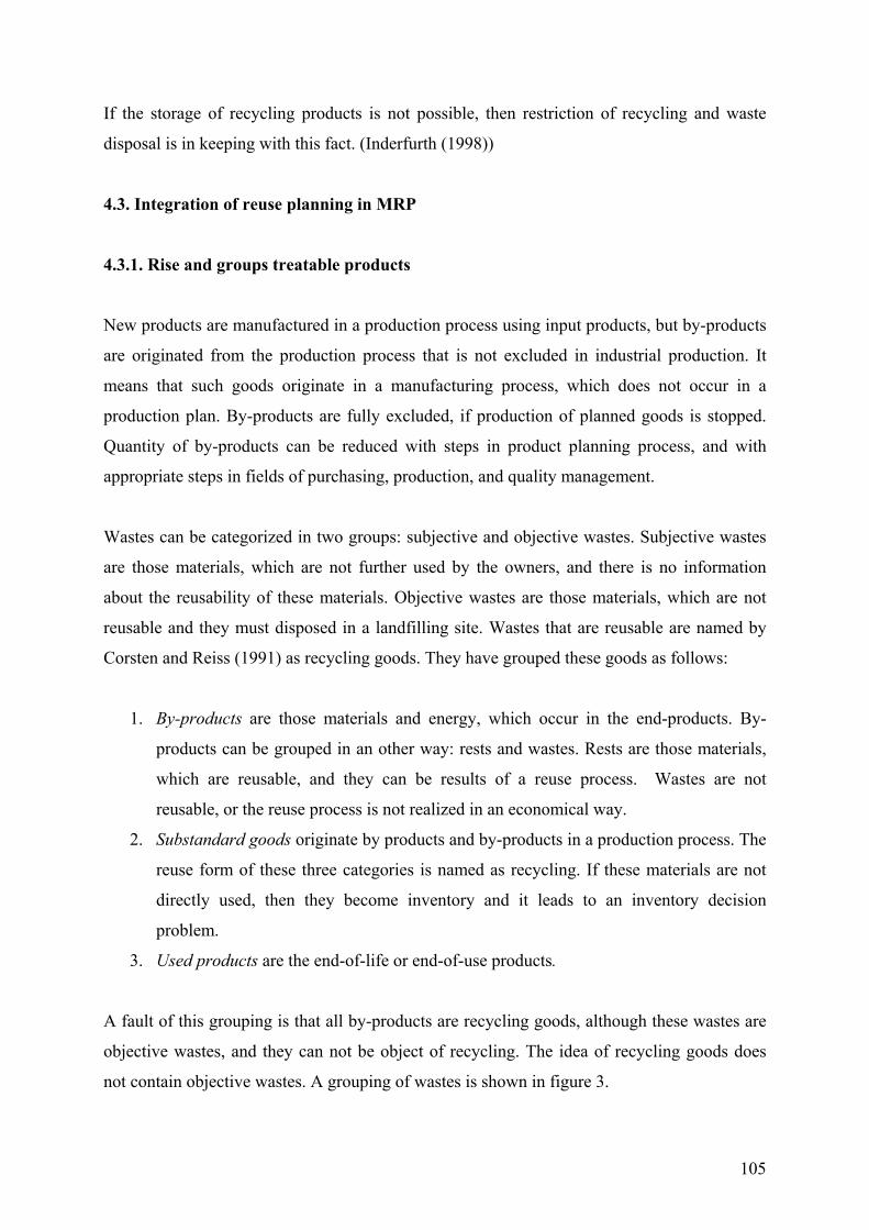
105
If the storage of recycling products is not possible, then restriction of recycling and waste
disposal is in keeping with this fact. (Inderfurth (1998))
4.3. Integration of reuse planning in MRP
4.3.1. Rise and groups treatable products
New products are manufactured in a production process using input products, but by-products
are originated from the production process that is not excluded in industrial production. It
means that such goods originate in a manufacturing process, which does not occur in a
production plan. By-products are fully excluded, if production of planned goods is stopped.
Quantity of by-products can be reduced with steps in product planning process, and with
appropriate steps in fields of purchasing, production, and quality management.
Wastes can be categorized in two groups: subjective and objective wastes. Subjective wastes
are those materials, which are not further used by the owners, and there is no information
about the reusability of these materials. Objective wastes are those materials, which are not
reusable and they must disposed in a landfilling site. Wastes that are reusable are named by
Corsten and Reiss (1991) as recycling goods. They have grouped these goods as follows:
1. By-products are those materials and energy, which occur in the end-products. By-
products can be grouped in an other way: rests and wastes. Rests are those materials,
which are reusable, and they can be results of a reuse process. Wastes are not
reusable, or the reuse process is not realized in an economical way.
2. Substandard goods originate by products and by-products in a production process. The
reuse form of these three categories is named as recycling. If these materials are not
directly used, then they become inventory and it leads to an inventory decision
problem.
3. Used products are the end-of-life or end-of-use products.
A fault of this grouping is that all by-products are recycling goods, although these wastes are
objective wastes, and they can not be object of recycling. The idea of recycling goods does
not contain objective wastes. A grouping of wastes is shown in figure 3.
106
Figure 3. Groups of reusable products (Becher-Roseman (1993)) 4.3.2. Process of collection and return
The reuse is come before collection of wastes in a firm. The collection of used products
realizes through physical and information connection of sources and destinations.
4.3.2.1. Collection
The first element of a return process is collection. Collection means the transportation of used
products to a collection place. Collection process is based on the planning information. Data
collection is a part of collection of used products, which is an information process. The
collection requirements are determined in this process including address of consumers and
due dates of transportation of collected goods and appliance. Further information is necessary
about type, age, and quality of used appliances. This information are the basis of a vehicle
routing planning, and disassembly and reuse planning process, i.e. these activities are the
planning basis of the collection.
There are three types of collection:
1. The collectors transport the used products to a collection place, that can be a
disassembly factory or a transfer place.
2. The owners of used products transport the materials to the collection place.
3. The combination of the above mentioned two strategies.
In general, the collection process is realized by waste transportation companies, although the
retailer firms take back the used products nowadays, if the consumer purchases a new one.
Treatable products
Wastes Reusable materials
Landfilling Rests Substandard goods Used products
107
Collection of data and used products has different problems:
1. There are parallel channels for consumers to collect data, and the supply is not
appropriate concrete.
2. Taking an order per telephone or data collection is not always possible. If it is
possible, then the waiting time is very long and after a number of trials.
3. The time between registration and collection can be more than a week because of the
attainability of these places.
4. The given due date can not be kept.
5. The collection means only the availability of products collected in containers, and not
the products stored in a house or in a cellar.
6. It is used such a vehicle, which capacity is not fully used.
7. The increase in collection systems leads to a competition for used products. The goal
is to maximize the utilization of collection systems and of reuse capacity. In this case
the collection routes become longer, and this means greater transportation costs and
environmental burden.
4.3.2.2. Loading
Loading is all transportation and storage process, which is loading and unloading vehicle with
products, and it emerges in case of change of transportation facilities. Loading is necessary in
a number of cases, in order to reduce the concentration of material flow. The loading is not
optional activity since there are direct and gradual return processes. Loading are realized
mainly with hand, which leads to high loading costs and to cause damages in used products.
4.3.2.3. Transportation
Transportation is determined as to get used products to a collection place or to a central
collection place. In a one-step return process transport means transportation of products to
assembly factory, and it is transportation of goods to next collection center in a several-step
return process. Other types of vehicles are used to transport than collect goods, in order to
reduce transportation costs. Transportation is not a forced activity in the return process, since
108
source and destination are the same places, if the distances are not so long and the collection
tour is ending at the destination. Transport is fulfilled by trucks.
The arising questions are the following:
1. The number of automotive and more effective loading processes is limited.
2. The used products can be damaged at loading and unloading processes, as in transport
process.
3. Moisture leads to corrosion, which reduces the disassembly of the products.
4. Auxiliary materials used in transportation are not storable, so there is no possibility to
store them in a place economical way.
4.3.2.4. Storage
Storage is a planned placing of usable products. The aim of storage is
1. to prevent the fluctuation of purchasing, transportation, and production,
2. to balance the difference between supply and demand,
3. to reduce the uncertainty of unknown supply and demand divergences,
4. to choice assortment.
There is output and input oriented storage. Output oriented storage concentrates on the
sources of used products, i.e. on owners, who will sell the used products. The input oriented
storage concentrates on the destination of used products, which is a disassembly factory. This
factory produces new inputs for the manufacturing process with dismantling.
4.3.2.5. Selection and assort
Selection of collected used products is the assort of products according to special disassembly
or reuse operation. The documentation of transportable used products is stored in addition to
concrete dismantling at this place This disassembly information plays an important role to
estimate the factory capacity and sales from the dismantled parts and modules. A preliminary
disassembly can be made in the selection process, so the efficiency of the transport process
can be increased and the disassembled quantity can be reduced. These two facts lead to a
109
better utilization of capacity. These supplement activities increase the demand for assort
factory providing special services. Assort is not a selection of products after type of machines
and modules, but it is an activity to support disassembly.
4.3.2.6. Packaging
Packaging has a function to prevent, to store, to transport, to identify, and to inform others
about the goods. This function necessitates the sale and use of products. One of the aims of
packaging activities is to achieve such a state, which do not pollute the environment in
process of packaging. It can be attained by use of such transportation facilities that requires
less or no packaging materials, i.e. containers.
The return process is influenced by the improvement programs and service level and quality.
It is important to know the consumer needs in return processes, for example service quality.
This determines the use level of built system and network, i.e. the demand for reverse
logistics services, which can reduce the costs of these services. (Waltemath, 2001)
4.3.3. Definition and types of recycling
Reuse is return of solid, liquid and gas state rests, substandard goods, and used products in the
manufacturing process. All firms are such systems that emit goods and wastes in the
environment, as output and absorb raw and other materials, and energy, as input. Jahnke
(1986) distinguishes internal, among firm, and external recycling.
1. Internal recycling means that products intended for recycling return to the
manufacturing firm. There is direct and indirect recycling. In case of direct recycling
the products are returned to the manufacturing process that they produced. Recycling
is indirect, if the return is preceded by a handling before production process.
2. Recycling among firm is defined as reuse of used products of other firms.
3. External recycling is the case when the product recycling is made by other firms.
4. Cooperative recycling can be defined, if not only used recycling products flow among
firms, but also planning and organizational information. This is a special case of
external and among firm recycling.
5. Manufacturing recycling is defined, as reuse of recycling products by their emittents.
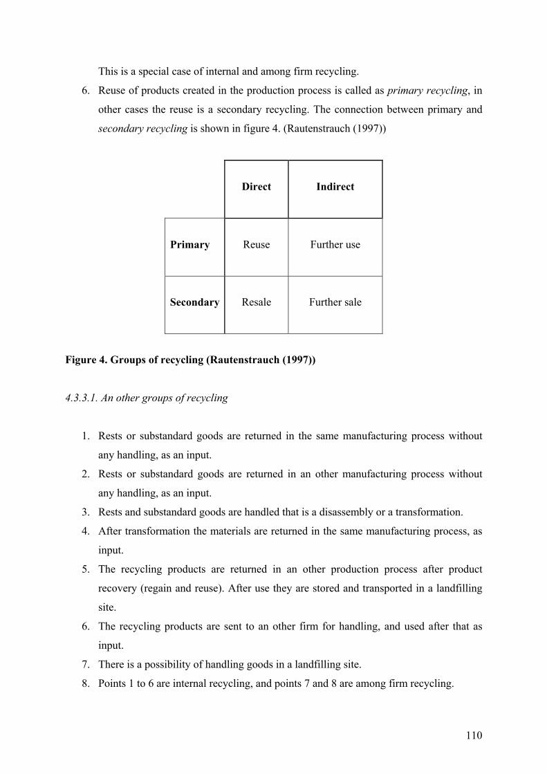
110
This is a special case of internal and among firm recycling.
6. Reuse of products created in the production process is called as primary recycling, in
other cases the reuse is a secondary recycling. The connection between primary and
secondary recycling is shown in figure 4. (Rautenstrauch (1997))
Direct
Indirect
Primary
Reuse
Further use
Secondary
Resale
Further sale
Figure 4. Groups of recycling (Rautenstrauch (1997))
4.3.3.1. An other groups of recycling
1. Rests or substandard goods are returned in the same manufacturing process without
any handling, as an input.
2. Rests or substandard goods are returned in an other manufacturing process without
any handling, as an input.
3. Rests and substandard goods are handled that is a disassembly or a transformation.
4. After transformation the materials are returned in the same manufacturing process, as
input.
5. The recycling products are returned in an other production process after product
recovery (regain and reuse). After use they are stored and transported in a landfilling
site.
6. The recycling products are sent to an other firm for handling, and used after that as
input.
7. There is a possibility of handling goods in a landfilling site.
8. Points 1 to 6 are internal recycling, and points 7 and 8 are among firm recycling.
111
Heterogeneity of rest materials and low concentration of rest materials are problems in reuse
process, which means the measure of use, corrosion, and level of hazardousness. Both factors
make more difficult the collection, storage, transportation, assort, and handling of materials.
(Corsten H., Reiss M., 1991)
4.3.3.2. Groups of recycling after processes
1. Production waste recycling is an internal recycling that touches the rests and
substandard products of manufacturing process.
2. Recycling during product use is a use of products in order to make the product partly
reusable.
3. Used material recycling is a different form recycling during product use. The
difference is that the product can not be as new recycled. These products are
dismantled and recovered, and as raw or other materials are returned in the production
process.
4.3.4. Objectives, conditions, tools and restrictions of recycling
4.3.4.1. Objectives
The objectives of recycling are the reduction of raw material and energy requirements, load of
environment, and saving of storage capacity through decrease and liquidation of wastes and
rest materials. The aim of a private enterprise is to reduce the requirements of raw materials,
and to lengthen the lifetime of recycling goods in a long run, in order to slow down the
creation rate of these goods, and to decrease the uncertainty.
Minimization of expensive capital investment causes the decrease of lifetime in development
of production process. This minimization includes the recycling, logistics, manufacturing,
planning, and transaction costs.
4.3.4.2. Conditions
The firm must consider a number of exogenous facts in reuse process, which restrict the
activity of the enterprise, for example:
112
1. the full recovery of raw materials from recycling goods is often not possible,
2. recycling goods are not reused with an intended frequency ,
3. not all recycling products are reusable economically,
4. environment injuring products originate in a recycling process,
5. reuse of certain goods is regulated by a law, so the use of these products is not a
decision problem.
Recycling can be seen, as a temporary relieve of use or consume of primary raw materials in
order to lengthen the lifetime of a product.
4.3.4.3. Tools
To investigate the tools used in recycling, there is a difference between application and
handling of recycling products:
1. Some of the recycling goods are reusable without any remanufacturing by the help of
assorts, transportation, and storage.
2. A selection or transformation procedure must be made in a handling process, which
can be a biological-technical or chemical-technical process, in order to make the
recycling products reusable.
A recycling decision model can be applied as a decision and planning model, if relevant
information about the recycling goods are available, e.g. price, quantity, and quantity of
recycling products. One of the factors influencing the decision complexity is the fundamental
goals, which can be a multidimensional goal function. In case of multidimensional goals there
is a conflict among the goals, and not only conflicts between ecological and economic
objectives.
The different groups of factors determine the next levels of complexity.
1.) Production process:
a) the lower and upper bounds are given for a usable quantity of recycling goods,
b) the fitting requirements of production and recycling process are known,
113
c) the return of recycling products in the same and other manufacturing processes is
known.
2.) Recycling products:
a) only rests, substandard goods, or used products or both of them are examined,
b) the beginning of recycling products can be continuous or discontinuous in time,
c) the storability of goods after heterogeneity, i.e. cleanness, form, color, or heat-
resistance etc.,
d) separability of parts and modules, material substitution.
3.) Reuse process:
a) depth of reuse process, i.e. level of dismantling and processing,
b) by-products of a reuse process, i.e. usable and unusable, damages and losses in reuse,
c) losses in quality.
The aim of a production planning and control system is to determine the production and
purchasing quantities in time under consideration of capacity restrictions, and handling steps
for deviation of planning, realization and control, in order to catch the fundamental goals.
4.3.4.4. Restrictions
1. Technical restrictions: recycling products are not usable without any frequency,
because the quality of goods deteriorates with the frequency of reuse. Further,
recycling goods are not fully reusable, because their decomposability is restricted
and dismantling is technically not possible.
2. Economic restrictions: costs caused by recycling can exceed its result, and the
savings in primary materials.
3. Ecological restrictions: recycling necessitates energy to transport recycling goods,
and often primary materials to refurbish their quality. Recycling is not useful from
ecological point of view, since recycling can cause environmental burden, which
exceeds the environmental utility.
4. Psychological restrictions: products manufactured from used products seem to have
a lower quality than new one, so the market reacts abstained with these products.
(Rautenstrauch (1998))
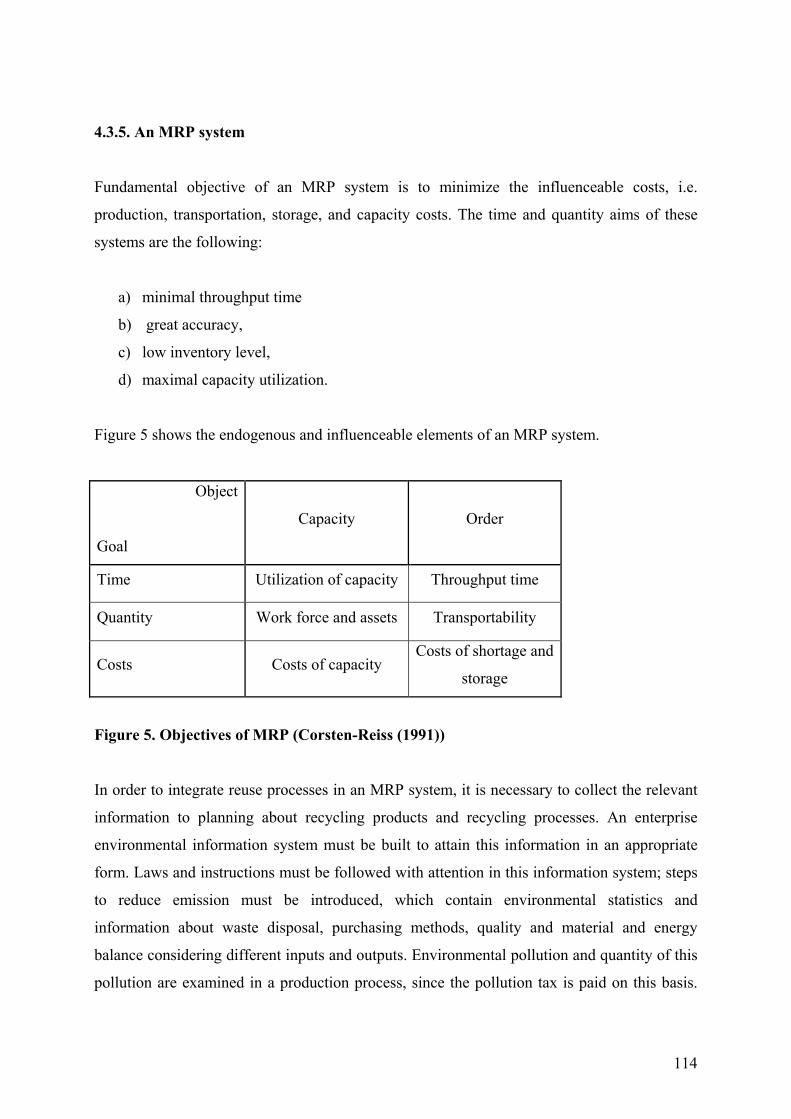
114
4.3.5. An MRP system
Fundamental objective of an MRP system is to minimize the influenceable costs, i.e.
production, transportation, storage, and capacity costs. The time and quantity aims of these
systems are the following:
a) minimal throughput time
b) great accuracy,
c) low inventory level,
d) maximal capacity utilization.
Figure 5 shows the endogenous and influenceable elements of an MRP system.
Object
Goal
Capacity Order
Time Utilization of capacity Throughput time
Quantity Work force and assets Transportability
Costs Costs of capacity Costs of shortage and
storage
Figure 5. Objectives of MRP (Corsten-Reiss (1991))
In order to integrate reuse processes in an MRP system, it is necessary to collect the relevant
information to planning about recycling products and recycling processes. An enterprise
environmental information system must be built to attain this information in an appropriate
form. Laws and instructions must be followed with attention in this information system; steps
to reduce emission must be introduced, which contain environmental statistics and
information about waste disposal, purchasing methods, quality and material and energy
balance considering different inputs and outputs. Environmental pollution and quantity of this
pollution are examined in a production process, since the pollution tax is paid on this basis.
115
Horizontal extension of an MRP system with a reuse process means three possible
generalizations:
1) recycling program planning,
2) recycling capacity planning,
3) recycling throughput planning.
I.) Breadth and depth of a recycling program is specified.
The following extension possibilities are in an MRP system:
1) Transportation and storage capacities must be considered, and priority rules have to
determine, in order to use the restrictedly storable products first.
2) Revision of transportation is necessary to consider the quantity and due date of
transportable recycling products. Immediate inclusion of not or only restrictedly
storable recycling products in the production process is very important. It is necessary
further to consider the manufacturing steps, quantity of recycling products, and due
dates in a manufacturing process. Emission limits have to be paid attention in case of
handling of not reusable by-products. Quantitative and qualitative criteria must be kept
in a further manufacturing.
II.) Quantity planning
Extension and transformation of an MRP system is necessary with quantity planning. Net
requirements of parts and raw materials are reduced by rests and wastes, and these reused
input goods are used as inputs in the production process, but rise of recycling goods means a
great uncertainty. Gross requirements are determined from material requirement planning.
There is an extension requirement in data handling and processing. It contains collection,
storage, refreshing, and processing of data connected with:
a) reliability (production time, quantity, and quality),
b) machines (waiting time),
c) work force (absence and presence time) and,
d) materials (shortage, and availability of materials at production places).
116
Of course, these materials must be available not only in the production, but also in the reuse
process. It is necessary a plan to group of recycling goods after quantity and type.
III.) Recycling throughput planning
The planning levels depend on one-sided each other in an MRP system, they follow each
other consecutively. Recycling process has a circular character, i.e. their processes are
independent from each other. Different steps of production planning are built up linearly, so
independence on planning levels is not considered. Performability of each steps depends on
precedents, i.e. each decision levels are conditions for the following decision levels.
Production program and capacity are connected with each other. If activities are realized with
independent throughput time from capacity, then this leads to an inconsistency in planning,
since quantities are fixed in quantity plan, and due date and capacity plans are not held for a
given due date, because due dates given in contracts do not correspond with necessary due
date. Since rest and waste materials return in not constant, but unsystematical quantities,
recycling makes more complex the estimation of due dates in a traditional MRP system.
Linearity of planning and cyclicality of planning object make more difficult the timeliness of
planning.
Reused products are used for net requirement. Factory and ordered products, spare parts and
safety stocks are used to cover gross requirement under recycling goods.
The measure of centralized decision must be mentioned in planning. If rests, wastes,
substandard goods, and used products appear in a recycling process, then the recycling
process is a multiple process, and the MRP system becomes more centralized. There is a
positive correlation between complexity and centralizedness. If a recycling process is more
uncertain, then an extended MRP system is less centralized. (Corsten-Reiss (1991))
4.3.6. MRP item record extended with recycling
The first part of an MRP item record extended with recycling is similar to that of traditional
MRP item record, although there is a recycled product stock line, which means that traditional
inventory line is extended with an alternative inventory. These stocks contain the spare parts
117
and materials recovered from returned items, and they become inventory. Then there is no
difference between reused and newly manufactured materials. Let us assume that the length of
planning horizon is 6 weeks, safety stock is 15 units, and lead time is 2 weeks. The data of
this example contain figure 6. The material flow is shown in figure 7.
The stock line is equal to the sum of produced, recycled, and initial stock level reduced with
gross requirements. The safety stock is 15 units, which is considered at the stock. The
expected level of returned items is 4 units. Recycling stock level is given. Recycling
requirements are equal to 4 units, which are the number of returned items. Recycling order
comes from recycling requirements with a leg of 2 weeks lead time. Handling requirement is
the stock level of recycling process reduced with recycling order. Planned order receipt is the
net requirement reduced with recycling requirement. Planned order release is planned order
receipt with a leg of lead time that is 2 weeks in our example.
0 1 2 3 4 5 6
Gross requirement 10 10 10 10 10 10
Produced stock 8 14
Recycled stock 5 4
Stock 9 12 20 15 15 15 15
Net requirement 3 0 5 10 10 10
Planned return 4 4 4 4 4 4
Recycling stock 7 4 4 4 4 4 4
Recycling requirement - - 5 4 4 4
Recycling order 5 4 4 4 - -
Handling requirement 2 0 0 0 - -
Planned order receipt - - 0 6 6 6
Planned order release 0 6 6 6 - -
Figure 6. MRP item record extended with recycling (Inderfurth-Jensen (1998))
118
Figure 7. Material flow in MRP item record
4.4. Summary
Environmental protection is become more important in enterprise praxis nowadays. Till
environmental protection is not a great business for firm, i.e. reverse logistics is not a factor of
competitive advantage; it can not be treated at a strategic level. It becomes competitive, if
society acknowledges environmental conscious activity supported with environmental audits
and the members of society purchase environment friendly products. Some of methods are
presented in this chapter, which help firm reduce the use of primary raw materials and energy,
as well environmental pollution. Firm can choose the best appropriate method from this
checklist. View of society must change in interest of environment. The government plays an
important role to influence the corporate strategy of firms. The saving of natural resources and
lengthen of use of natural resources support to achieve a sustainable development path in
interest of future generations.
Recycling stock
End-product stock Demand
Production
Recycling
119
5. Summary and Further Research
Reverse logistics and its application in production planning are investigated in this work.
Reverse logistics can completely built in material requirements planning (MRP) systems. The
extension is that classical MRP item records contain the files of returned and reusable
products in addition to traditional information. Last rows of MRP item records show the
requirements of previous production phases and/or purchasing. The inventory problem occurs
at this level, whether the decision maker must unite production and/or purchasing lots, or not.
It is used heuristics in traditional MRP systems to determine the lot sizes, as Groff-algorithm,
or Silver-Meal heuristics, and so on. These heuristics apply the optimality conditions of EOQ
model. This property is that the ordering and/or setup costs are equal to the inventory holding
costs in cot minimum. The question is now, whether EOQ-type reverse logistic inventory
models are applied to lot sizing in extended MRP systems.
To answer the last question, I have presented six reverse logistic EOQ-type inventory models.
The models have common conditions, that are the exclusion of shortage. The cost structure is
similar to that of classical EOQ model, i.e. there are cycle fix purchasing/production costs,
inventory holding costs for new products, and fix and holding costs for reusable items.
I have investigated the examined models under these conditions, I have shown that the models
lead to a meta-model presented in appendix. I can simplify the cost function after its
construction with two equalities. Either the number of lots or the lot sizes can be substituted in
the cost function. If the number of batches is substituted in the cost function, then the
variables are the lot sizes and the problem that the number of lots is integer can not be studied
in the model further. This is the reason why it is more simply to substitute the lot sizes in cost
function. With the help of this method I have shown such an example, where purchasing and
reuse lot numbers are strictly greater than one.
I have examined those cases, when EOQ-type and non EOQ-type linear
purchasing/manufacturing, reuse, and waste disposal costs are included in the cost function.
For this type of models I have shown that waste disposal is neglected in the optimal solution,
i.e. all returned and reusable items are economical to reuse. The necessary and sufficient
120
condition for reusability of all used items is that one of the pure strategies, i.e. only
purchasing/manufacturing and complete reuse, is cost minimal.
The presented inventory models can be the basis for those heuristics, which are applicable in
extended MRP systems. As I know, there is no publication on this field. The generalization of
Wagner-Whitin dynamic lot size model with reuse was undertaken by Richter-Sombrutzki
(2000), Richter-Weber (2001) and Richter-Gobsch (2005).
I present the generalized model of Richter-Sombrutzki (2000), which is the extension of
model of Schrady (1967) for the case of time varying demand and return. In this model there
is no waste disposal activity. The parameters and variables are different that of published
article, and they are the same, as they were introduced by Schrady (1967).
The stock-flow identity relations are the following:
tRttt
tRt
Pttt
RQii
DQQII
+−=
−++=
−
−
1
1 , (t = 1,2,…,T)
.0,0
,0,0
≥≥
≥≥Rt
Pt
tt
iI, (t = 1,2,…,T)
where I0 = i0 =0. The first equality is the balance connection in tth period for new products,
i.e. the inventory level at the end of period t is equal to the sum of initial inventory level,
purchasing and repair reduced with demand. The second equation includes the returned items
and the items taken in reuse process. The last inequalities are the nonnegativity conditions of
variables.
The cost function is
( ) min1
21 →⋅+⋅+⋅+⋅∑=
T
tt
RtRt
PtP ihQsignAIhQsignA .
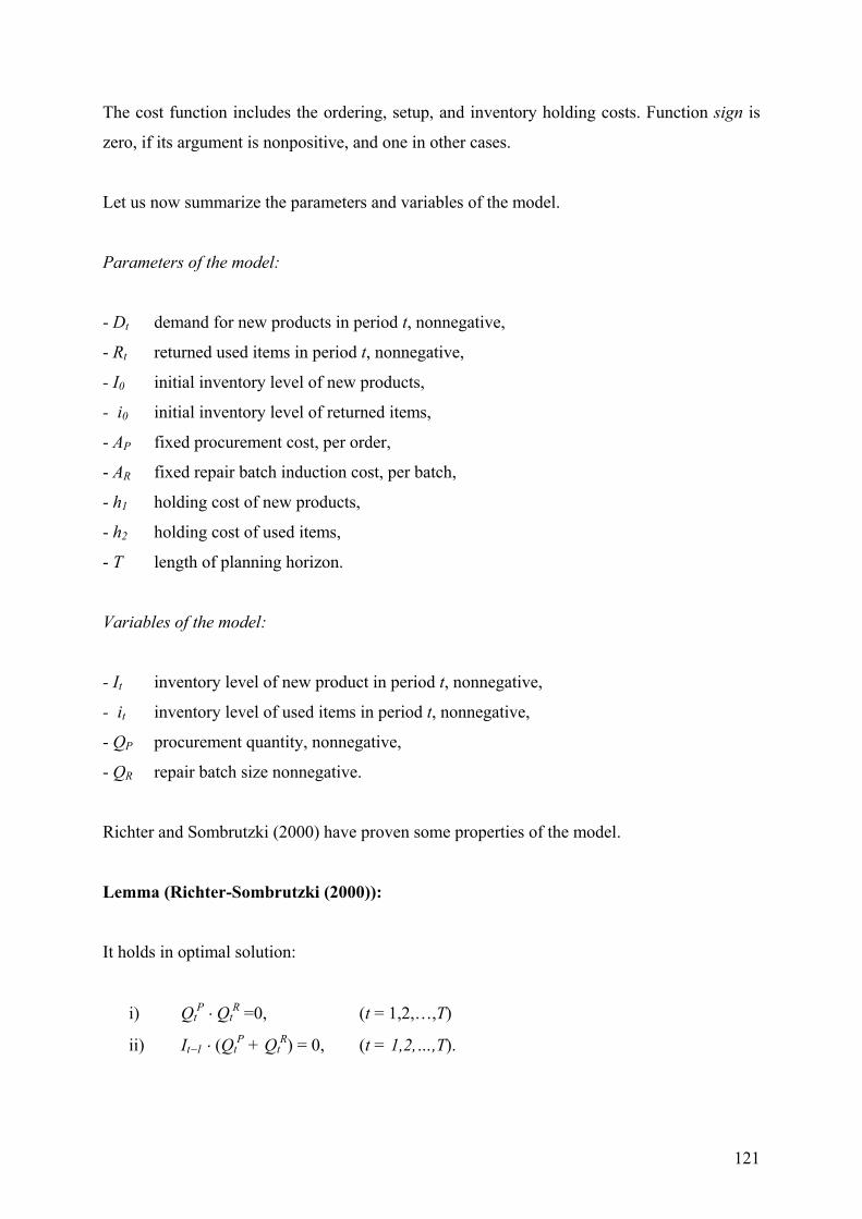
121
The cost function includes the ordering, setup, and inventory holding costs. Function sign is
zero, if its argument is nonpositive, and one in other cases.
Let us now summarize the parameters and variables of the model.
Parameters of the model:
- Dt demand for new products in period t, nonnegative,
- Rt returned used items in period t, nonnegative,
- I0 initial inventory level of new products,
- i0 initial inventory level of returned items,
- AP fixed procurement cost, per order,
- AR fixed repair batch induction cost, per batch,
- h1 holding cost of new products,
- h2 holding cost of used items,
- T length of planning horizon.
Variables of the model:
- It inventory level of new product in period t, nonnegative,
- it inventory level of used items in period t, nonnegative,
- QP procurement quantity, nonnegative,
- QR repair batch size nonnegative.
Richter and Sombrutzki (2000) have proven some properties of the model.
Lemma (Richter-Sombrutzki (2000)):
It holds in optimal solution:
i) QtP ⋅ Qt
R =0, (t = 1,2,…,T)
ii) It−1 ⋅ (QtP + Qt
R) = 0, (t = 1,2,…,T).
122
I do not prove these properties, it can be found in above mentioned paper. Condition (i) says
that both repair and purchasing can not occur in a period in optimal solution. The second
equation expresses that purchasing or repair occurs only those periods, when initial inventory
level is zero. If the initial inventory level is zero, then purchasing or repair must occur. This
property is similar that of Wagner-Whitin dynamic lot size model, i.e.
procurement/production occurs in periods with zero initial inventory level. As we see, the
inventory holding policy offered by Schrady (1967) applies these two properties. This
dynamic model can be solved with method of dynamic programming, but the solution is very
time consuming for relatively small problem, so construction of heuristics to create
suboptimal solution is necessary.
A need for further research is obvious, but the question is whether EOQ-type reverse logistic
models are appropriate to construct a suboptimal solution of extended Wagner-Whitin
models, i.e. to create with it satisfactory lot sizes for repair and purchasing. And now a
question is how to construct such an algorithm.
The next group of question is; if there are effective heuristics, then how they function. For
which cost and system parameters offer the algorithms a satisfactory solution? To test the
effectiveness of algorithms, it is necessary to make simulations. Without any numerical
analysis we can not answer this question. These offered heuristics can be used in production
planning and MRP systems.
123
References
1. Arrow, K.J., Enthoven, A.C. (1961): Quasi-concave programming, Econometrica,
Vol. 29, No. 4, 779-800
2. Arrow, K.J., Karlin, S. (1958): Production over Time with Increasing Marginal
Costs, In: K.J. Arrow, S. Karlin, H.Scarf (Eds.): Studies in the Mathematical Theory
of Inventory and Production, Stanford Univ. Press, Stanford, 61-69
3. Becher J., Rosemann M. (1993): Logistik und CIM, Springer-Verlag, Berlin et al.
4. Carter, C. R.- Ellram, L. M. (1998): Reverse logistics: A review of the literature and
framework for future investigation, Journal of Business Logistics,. No.1., 85-101.
5. Corsten H., Reiss M. (1991): Recycling in PPS-Systemen, Die Betriebswirtschaft,
615-627
6. Cselényi J.- Mang B.- Bányainé Tóth Á.- Bányai T. (1997): A recycling logisztika,
mint a logisztikai kutatások dinamikusan fejlődő egyik új iránya, Logisztika, 1. sz.,
8-13.
7. de Brito, M. P. – Dekker, R. (2004): A framework for reverse logistics, In: Dekker,
R.- Fleischmann, M. – Inderfurth, K. – van Wassenhove, L. (2004, Eds.): Reverse
Logistics: Quantitative Models for Closed-Loop Supply Chains, Springer- Berlin et
al., 3-27
8. Dobos, I. (1999): Production-Inventory Strategies for a Linear Reverse Logistics
System, Discussion Paper 431, Faculty of Economics and Business Administration,
University Bielefeld.
9. Dobos, I. (2001): Optimal inventory strategies for EOQ-type reverse logistics
systems, Working Paper Nr. 1, Department of Business Economics, Budapest
University of Economics and Public Administration
10. Dobos, I. (2002): The generalization of SCHRADY´s model: a model with repair,
Working Paper Nr. 7, Department of Business Economics, Budapest University of
Economics and Public Administration
11. Dobos, I. (2002): The optimality of Richter´s model of repair and waste disposal,
Working Paper Nr. 10, Department of Business Economics, Budapest University of
Economics and Public Administration
12. Dobos, I. (2003a): Comparison of disposal strategies in linear reverse logistics
models, Working Paper Nr. 41, Department of Business Economics, Budapest
124
University of Economics and Public Administration
13. Dobos, I. (2003b): Optimal production-inventory strategies for a HMMS-type
reverse logistics system, International Journal of Production Economics 81-82, 351-
360
14. Dobos I. (2004): Készletmodellek a visszutas logisztikában, In: Czakó E., Dobos I.,
Kőhegyi A. (Szerk.): Vállalatai versenyképesség, logisztika, készletek:
Tanulmányok Chikán Attila tiszteletére, BKÁE Vállalatgazdaságtan tanszék,
(2004), Budapest, 290-303
15. Dobos, I., Kistner, K.-P. (2000): Production-Inventory Control in a Reverse
Logistics System, Proceedings of the 11th Int. Working Sem. on Prod. Econ.,
Igls/Innsbruck, 2000, Austria, Pre-Prints Vol. 2., 67-86
16. Dobos, I., Richter, K. (1999a): Comparison of Deterministic One-Product Reverse
Logistics Models, in: Hill, R., Smith, D. (Eds.): Inventory Modelling: A Selection of
Research Papers Presented at the Fourth ISIR Summer School (1999), Exeter 1999,
69-78
17. Dobos, I., Richter, K. (1999b): A Remanufacturing Model Reconsidered: A
Technical Note, Discussion paper Nr. 128 (1999), Wirtschaftswissenschaftliche
Fakultät, Europa-Universität Viadrina Frankfurt (Oder)
18. Dobos, I., Richter, K. (1999c): The number of batch sizes in a remanufacturing
model, Discusion paper 132, Viadrina European University of Frankfurt (Oder),
Faculty of Economics and Business Administration.
19. Dobos, I., Richter, K. (2000): The integer EOQ repair and waste disposal model –
further analysis. Central European Journal of Operations Research 8, 173-194
20. Dobos, I., Richter, K. (2003): A production/recycling model with stationary demand
and return rates, Central European Journal of Operations Research 11, 35-46
21. Dobos, I., Richter, K., (2004): An extended production/recycling model with
stationary demand and return rates, International Journal of Production Economics
90, 311-323
22. Dobos, I., Richter, K., (2006): A production/recycling model with quality
considerations, Int. J. of Production Economics, to appear
23. Feichtinger, G., Hartl, R.F. (1986): Optimale Kontrolle ökonomischer Prozesse:
Anwendungen des Maximumprinzips in den Wirtschaftswissenschaften, de Gruyter,
Berlin
125
24. Ferrer, G., Whybark, D. C. (2000): Material Planning for a Remanufacturing
Facility, Production and Operations Management Vol. 10, 112-124
25. Fleischmann, M., Bloemhof-Ruwaard, J.M., Dekker, R., van der Laan, E. van
Nunen, J.A.E.E., van der Wassenhove, L.N. (1997): Quantitative models for reverse
logistics: a review. European Journal of Operational Research 103, 1-17
26. Gupta, M. C.(1995), Environmental management and its impact on the operations
function, Int. Journal of Operations & Decision Management 15(8): 34-51
27. Grím, T., Dobos, I. (2006): Termeléstervezés a visszutas logisztikában,
Vezetéstudomány, megjelenés alatt
28. Guide, V.D.R. (2000): Production planning and control for remanufacturing:
industry practice and research needs, Journal of Operations Management 18, 467-
483
29. Hill, R.M. (1996): Optimizing a production system with fixed delivery schedule,
Journal of the Oper. Research Society 47, 954-960
30. Holt, C.C., Modigliani, F., Muth, J.F., Simon, H.A. (1960): Planning Production,
Inventories, and Work Forces, Prentice-Hall, Englewood Cliffs, N.J.
31. Inderfurth K. (1998): Neue Aufgaben und Lösungsansatze der Produktionsplanung
bei Produktrecycling, Preprint Nr. 26, Fakultät für Wirtschaftwissenschaften, Otto-
von-Guericke Universität, Magdeburg
32. Inderfurth, K., Jensen, T. (1998): Analysis of MRP policies with recovery options,
10th Int. Working Sem. on Production Economics, Innsbruck/Igls, Austria, Pre-
Prints Vol. 2., 265-300
33. Jahnke, B. (1986): Betriebliches Recycling: Produktionswirtschaftliche Probleme
und betriebwirtschaftliche Konsequenzen, Gabler-Verlag, Wiesbaden
34. Kelle, P., Silver, E.A. (1989): Purchasing policy of new containers considering the
random returns of previously issued containers, IIE Transactions 21(4): 349-354
35. Kistner, K.-P., Dobos, I. (2000): Optimal Production-Inventory Strategies for a
Reverse Logistics System, In: Dockner, E. J. , Hartl, R. F., Luptacik, M., Sorger, G.
(Eds.): Optimization, Dynamics, and Economic Analysis: Essays in Honor of
Gustav Feichtinger, Physica-Verlag, Heidelberg, New York, 246-258
36. Kleber, R., Minner, S., Kiesmüller, G. (2002): A continuous time inventory model
for a product recovery system with multiple options, International Journal of
Production Economics 79, 121-141
37. Koh, S.-G., Hwang, H., Sohn, K.-I., Ko, C.-S. (2002): An optimal ordering and
126
recovery policy for reusable items, Computers & Industrial Engineering 43, 59-73
38. Kohut, Zs., Nagy, A. (2004): A logisztika környezetvédelmi vonatkozása: A
visszutas logisztika, Összhangban az elmélet és a gyakorlat?, TDK - dolgozat,
BKÁE, Vállalatgazdaságtan Tanszék, Budapest
39. Kohut, Zs., Nagy, A., Dobos, I. (2005): Visszutas logisztika: Egy fogalmi keret,
Vezetéstudomány , 36, 47-54
40. Kopicky, R. J. – Berg, M. J. – Legg, L. – Dasappa, V. – Maggioni, C. (1993): Reuse
and recycling: Reverse logistics opportunities, Council of Logistics Management,
Oak Brook, IL
41. Krumwiede, Dennis W.-Sheu, Chwen: A model for reverse logistics entry by third-
party providers, Omega 30, 2002, 325-333
42. Lambert, D.M., Stock, J.R. (1981): Strategic Physical Distribution Management,
Irwin, Homewood, IL
43. Mabini, M.C., Pintelon, L.M., Gelders, L.F. (1998): EOQ type formulation for
controlling repairable inventories. International Journal of Production Economics
54, 173-192
44. Mike, G. (2002): A logisztika környezetvédelmi kérdései és a Reverse Logistics, 19.
sz. műhelytanulmány BKÁE, Vállalatgazdaságtan Tanszék, Budapest
45. Minner, S., Kleber, R. (2001): Optimal Control of Production and Remanufacturing
in a Simple Recovery Model with Linear Cost Functions, OR Spektrum 23, 3-24
46. Murphy, P.R., Poist, R.P. (1989): Managing of logistics retromovements: An
empirical analysis of literature suggestions, Transportation Research Forum, Vol.
29, No. 1, 177-184
47. Nahmias, N., Rivera, H.: (1979): A deterministic model for repairable item
inventory system with a finite repair rate. International Journal of Production
Research 17(3), 215-221
48. Pohlen, T. L.- Farris, M. (1992): Reverse logistics in plastic recycling, International
Journal of Physical Distribution and Logistics Management, Vol. 22, No. 7., pp. 35-
47.
49. Rautenstrauch C. (1997): Fachkonzept für ein integriertes Produktions-,
Recyclingplanungs- und Steuerungsystem (PrPS), Walter de Gruyter, Berlin
50. Richter, K. (1994): An EOQ repair and waste disposal model, Proceedings of the
Eight International Working Seminar on Production Economics, Vol. 3, 83-91,
Igls/Innsbruck
127
51. Richter, K. (1996a): The EOQ repair and waste disposal model with variable set-up
numbers, European Journal of Operational Research 96, 313-324
52. Richter, K. (1996b): The extended EOQ repair and waste disposal model,
International Journal of Production Economics 45, 443-447
53. Richter, K. (1996c): Modellierung von kombinierten Wiederverwendungs- und
Entsorgungsprozessen, in: H. Wildemann (Ed.): Produktions- und
Zuliefernetzwerke, TCW Transfer-Centrum-Verlag München, 279-291
54. Richter, K. (1997): Pure and mixed strategies for the EOQ repair and waste disposal
problem, OR Spektrum 19, 123-129
55. Richter, K., Dobos I. (1996): Solving the integer EOQ repair and waste disposal
problem, In: Flapper, S. D., de Ron, A. J. (Eds.): Proceedings: First International
Working Seminar on Reuse (1996), Eindhoven, 247-255
56. Richter, K., Dobos, I. (1999): Analysis of the EOQ repair and waste disposal model
with integer setup numbers, International Journal of Production Economics 59, 463-
467
57. Richter, K., Dobos I. (2003a): Az újrahasznosítás hatása a gazdasági
sorozatnagyságra, Szigma XXXIV. (2003), 45-63
58. Richter, K., Dobos, I. (2003b): A Reverse Logistics Model with Integer Setup
Numbers, In: Leopold-Wilbdurger, U., Rendl, F., Wäscher, G. (Eds.): Operations
Research Proceedings 2002: Selected Papers of the International Conference on
Operations Research (SOR 2002), Springer-Verlag, Berlin, Heidelberg, New York,
95-101
59. Richter, K., Dobos, I. (2004): Production-inventory control in an EOQ-type reverse
logistics system, In: Dyckhoff, H., Lackes, R., Reese, J. (Eds.): Supply Chain
Management and Reverse Logistics, Springer Verlag, Berlin et al., 139-160
60. Richter, K., Gobsch, B. (2005): Kreislauf-Logistik mit Losgrössenrestriktionen,
Zeitschrift für Betriebswirtschaft-Special Issue 4/2005, 57-78
61. Richter, K., Sombrutzki, M. (2000): Remanufacturing planning by reverse
Wagner/Whitin models, European Journal of Operational Research 121, 304-315
62. Richter, K., Weber, J. (2001): The reverse Wagner/Whitin modell with variable
manufacturing and remanufacturing cost, Int. J. of Production Economics 71, 447-
456
63. Rixer, A. (1995): Az inverz logisztika és a logisztika, mint körfolyamat,
Közlekedéstudományi Szemle XLV., 166-175
128
64. Rogers, D. S. -Tibben-Lembke, R. S. (1999): Going Backwards: Reverse Logistics
Trends and Practices, Reverse Logistics Executive Council, Pittsburgh
65. Schrady, D.A. (1967): A deterministic inventory model for repairable items, Naval
Research Logistic Quarterly 14, 391-398
66. Seierstad, A., Sydsaeter, K. (1987): Optimal Control Theory with Economic
Applications, Noth-Holland, Amsterdam
67. Spengler T., Püchert H., Penkuhn T., Rentz O. (1997): Environmental Integrated
Production and Recycling Management, European Journal of Operational Rearch
97, 308-326
68. Stock, J. R (1998): Development and Implementation of Reverse Logistics Program,
Council of Logistics Management, Oak Brook, IL
69. Stock, J. R. (1992): Reverse Logistics, Council of Logistics Management, Oak
Brook, IL
70. Takayama, A. (1985): Mathematical Economics, Cambridge University Press,
Cambridge et al.
71. Teunter, R., van der Laan, E. (2002): On the non-optimality of the average cost
approach for inventory models with remanufacturing, International Journal of
Production Economics 79, 67-73
72. Teunter, R.H. (2001): Economic Ordering Quantities for Recoverable Item
Inventory Systems, Naval Research Logistics, Vol. 48, 484-495
73. Teunter, R. (2004): Lot-sizing for inventory systems with product recovery,
Computers & Industrial Engineering 46, 431-441
74. Thierry, M. - Salomon, M. J. - van Nunen, J. - van Wassenhove, L. (1995): Strategic
Issues in Product Recovery Management, California Management Review, Vol. 37.,
No. 2., pp. 114-135.
75. Thompson, G.L., Sethi, S.P. (1980): Turnpike Horizons for Production Planning,
Management Science 26, 229-241
76. Vörösmarty, Gy., Dobos, I. (2003): Purchasing Strategies in Reverse Logistics
Systems, In: Chikán, A. (Eds.): Proceedings of the 12th International IPSERA
Conference, Budapest, (2003), 1082-1088
77. Waltemath, A.. M. (2001): Altproduktrückfürung als logistische Dienstleistung,
Dissertation, Technische Universität, Berlin
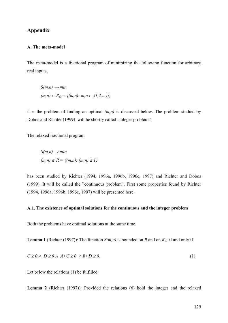
129
Appendix
A. The meta-model
The meta-model is a fractional program of minimizing the following function for arbitrary
real inputs,
S(m,n) → min
(m,n) ∈ RG = {(m,n): m,n ∈ {1,2,...}},
i. e. the problem of finding an optimal (m,n) is discussed below. The problem studied by
Dobos and Richter (1999) will be shortly called ”integer problem”.
The relaxed fractional program
S(m,n) → min
(m,n) ∈ R = {(m,n): (m,n) ≥ 1}
has been studied by Richter (1994, 1996a, 1996b, 1996c, 1997) and Richter and Dobos
(1999). It will be called the ”continuous problem”. First some properties found by Richter
(1994, 1996a, 1996b, 1996c, 1997) will be presented here.
A.1. The existence of optimal solutions for the continuous and the integer problem
Both the problems have optimal solutions at the same time.
Lemma 1 (Richter (1997)): The function S(m,n) is bounded on R and on RG if and only if
C ≥ 0 ∧ D ≥ 0 ∧ A+C ≥ 0 ∧ B+D ≥ 0. (1)
Let below the relations (1) be fulfilled:
Lemma 2 (Richter (1997)): Provided the relations (6) hold the integer and the relaxed
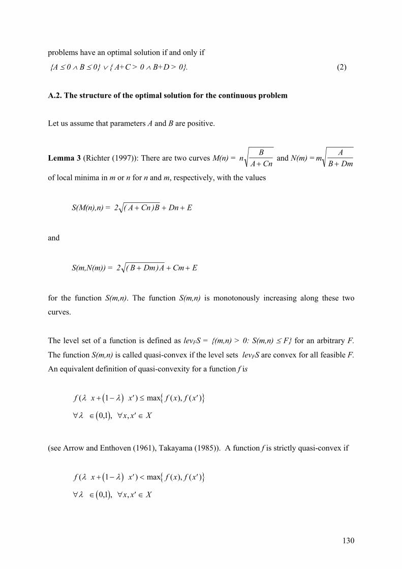
130
problems have an optimal solution if and only if
{A ≤ 0 ∧ B ≤ 0} ∨ { A+C > 0 ∧ B+D > 0}. (2)
A.2. The structure of the optimal solution for the continuous problem
Let us assume that parameters A and B are positive.
Lemma 3 (Richter (1997)): There are two curves M(n) = nB
A Cn+ and N(m) =m
AB Dm+
of local minima in m or n for n and m, respectively, with the values
S(M(n),n) = 2 ( )A Cn B Dn E+ + +
and
S(m,N(m)) = 2 ( )B Dm A Cm E+ + +
for the function S(m,n). The function S(m,n) is monotonously increasing along these two
curves.
The level set of a function is defined as levFS = {(m,n) > 0: S(m,n) ≤ F} for an arbitrary F.
The function S(m,n) is called quasi-convex if the level sets levFS are convex for all feasible F.
An equivalent definition of quasi-convexity for a function f is
( ) { }
( )
f x x f x f x
x x X
( ) max ( ), ( )
, , ,
λ λ
λ
+ − ′ ≤ ′
∀ ∈ ∀ ′ ∈
1
0 1
(see Arrow and Enthoven (1961), Takayama (1985)). A function f is strictly quasi-convex if
( ) { }
( )
f x x f x f x
x x X
( ) max ( ), ( )
, , ,
λ λ
λ
+ − ′ < ′
∀ ∈ ∀ ′ ∈
1
0 1
131
Below some example of the level set for a quasi-convex function is given.
Theorem 1: If the relation A > 0, B > 0, C+D ≥ 0 holds then function S(m,n) is strictly
quasi-convex.
Proof: To prove the theorem, let us check the conditions of strictly quasi-convexity. It follows
from the definition of quasi-convexity, that the function F f x x x( ) ( ( ))λ λ= ′ + − ′ has no
maximum between 0 and 1. Let us investigate our problem in the following form:
( ) ( )G Am mn n
Bn nm m
C m m D n n E( )λλλ
λλ
λ λ=+
++
+
++ + + + +
∆∆
∆∆
∆ ∆ ,
where (m,n)>(0,0) is an arbitrary point, and (∆m,∆n) a feasible direction. We must now
prove, that function G(λ) has no maximum for every (m,n) and (∆m,∆n).
(i) ∆m < 0, ∆n > 0
In this case the function
m mn n
mmn
n
n nmn
+
+=
−
++
λλ λ∆∆
∆∆∆
∆∆
is convex because the numerator is positive, and the function
n nm m
nnm
m
m mnm
+
+=
−
++
λλ λ∆∆
∆∆∆
∆∆
is also convex, because value ∆m is negative. The other functions are linear and convex, and
the function G(λ) is convex and has no maximum for every λ>0. The case ∆m>0, ∆n<0 can
be handled similarly.
132
(ii) ∆m > 0, ∆n > 0, n∆m-n∆m > 0
Let us now investigate the derivative of function G(λ). We will show that the function has a
minimum, if any.
( ) ( )
′ =−
++
−
++ +G A
n m m n
n nB
m n n m
m mC m D n( )λ
λ λ
∆ ∆
∆
∆ ∆
∆∆ ∆2 2
The case is considered when the function G(λ) is monotonously non-decreasing. Then
( ) ( )( )
( )( ) ( )A n m m nm m
n nC m D n m m B n m m n∆ ∆
∆
∆∆ ∆ ∆ ∆ ∆−
+
+≥ − + + + −
λ
λλ
2
2
2
The left-hand side function is monotonously increasing, and the quadratic function is
monotonously decreasing because of the non-negativity of parameters C and D. (It is easy to
check with derivation.) There exists one and only one λ0 satisfying the equality, if
( ) ( ) ( )A n m m n mn
C m D n n B n m m n∆ ∆ ∆ ∆ ∆ ∆− ≥ − + + −2
22 .
It means, that on the interval λ>λ0 the function is monotonously increasing, and
monotonously decreasing in other case. If value λ0 does not exist, then the function G(λ) is
monotonously increasing for every nonnegative λ. And we have proved of the theorem.
In case of quasi-convex programming the following theorem provides a necessary and
sufficient condition of optimality. A variable is called relevant, if it can take on a positive
value without necessarily violating the constraints.
Theorem 2. (Arrow and Enthoven (1961), Takayama (1985)): Let f(x) be a differentiable
quasi-convex function of the n-dimensional vector x, and let g(x) be an m-dimensional
differentiable quasi-convex vector function, both defined for x ≥ 0. Let x0 and λ0 satisfy the
Kuhn-Tucker-Lagrange conditions, and let one of the following conditions be satisfied:
133
(a) f xi00> for at least one variable xi0
;
(b) f xi10< for some relevant variable xi1 ;
(c) f x ≠ 0 and f(x) is twice differentiable in the neighborhood of x0;
(d) f(x) is convex.
Then x0 minimizes f(x) subject to the constraints g(x) ≤ 0, x ≥ 0.
Proof is omitted; see Arrow and Enthoven (1961).
Let us now check condition (c) of Theorem 2 to our problem.
Lemma 4: Let point (m0, n0) ≥ (1, 1). Then
(a)
( )
≠
++−
+−=
00
1
1
020
0
20
0
0
00
Dm
Bnm
A
Cmn
Bn
A
nSmS
nm∂∂∂∂
;
(b)
( )
−−
−−=
30
020
20
20
20
30
0
00
2
22
2
2
2
211
112
nm
Am
Bn
A
mB
nA
mn
B
nS
mnS
nmS
mS
nm∂∂
∂∂∂
∂∂∂
∂∂
.
The proof of the lemma is easy and is left to the reader.
As it is shown, our continuous auxiliary problem is a quasi-convex, and the function S(m,n)
satisfies the condition (c) of Theorem 2. This condition guarantees the optimal solution. An
example of the function S(m,n) in shown in Fig. 1.
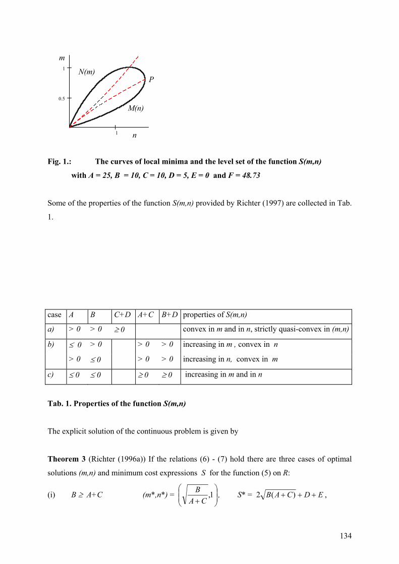
134
1
0.5
1
Fig. 1.: The curves of local minima and the level set of the function S(m,n)
with A = 25, B = 10, C = 10, D = 5, E = 0 and F = 48.73
Some of the properties of the function S(m,n) provided by Richter (1997) are collected in Tab.
1.
case A B C+D A+C B+D properties of S(m,n)
a) > 0 > 0 ≥ 0 convex in m and in n, strictly quasi-convex in (m,n)
b) ≤ 0 > 0 > 0 > 0 increasing in m , convex in n
> 0 ≤ 0 > 0 > 0 increasing in n, convex in m
c) ≤ 0 ≤ 0 ≥ 0 ≥ 0 increasing in m and in n
Tab. 1. Properties of the function S(m,n)
The explicit solution of the continuous problem is given by
Theorem 3 (Richter (1996a)) If the relations (6) - (7) hold there are three cases of optimal
solutions (m,n) and minimum cost expressions S for the function (5) on R:
(i) B ≥ A+C (m*,n*) =
+1,
CAB , S* = EDCAB +++ )(2 ,
n
m
M(n)
N(m) P
135
(ii) A-D ≤ B≤ A+C (m*n*) = (1,1), S* = A+B+C+D+E
(iii) A ≥ B+D (m*,n*) =
+ DBA,1 , S* = ECDBA +++ )(2 .
A.3. The optimal solution for the integer problem
A.3.1. The cases a) in Tab. 1
Lemma 5: Let in Theorem 1 to the condition (i) additionally 49A ≤ 527C or to (iii)
additionally 49B ≤ 527D be fulfilled. Then the optimal integer solution is on the line n = 1
or on the line m=1, respectively.
Proof: Let the case (iii) be considered. Let us assume, that S(1,n) ≥ S(1,n+1) and the optimal
continuous solution is (1,n*). Let n+1 = n*+δ. It can be shown by elementary operations
that
( )S n A B D C E A B D
n n( , ) ( ) ( )
* *1 1 2
2
+ = + + + + ++
δδ
,
where 0 < δ < 0.5. Let the following problem be investigated:
sup* ( * )* . , .n n n≥ < < +
1 5 0 0 5
2
δ
δδ
.
The function is monotonously increasing in δ and monotonously decreasing in n*. Then
( )δ
δ
21
12n n* * +≤ ,
and
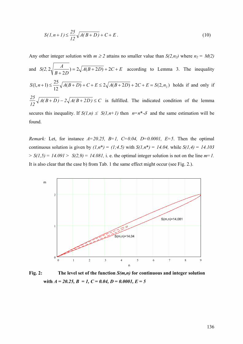
136
S n A B D C E( , ) ( )1 1 2512
+ ≤ + + + . (10)
Any other integer solution with m ≥ 2 attains no smaller value than S(2,n2) where n2 = M(2)
and S(2, ECDBADB
A+++=
+2)2(2)
22 according to Lemma 3. The inequality
),2(2)2(2)(1225)1,1( 2nSECDBAECDBAnS =+++≤+++≤+ holds if and only if
2512
2 2A B D A B D C( ) ( )+ − + ≤ is fulfilled. The indicated condition of the lemma
secures this inequality. If S(1,n) ≤ S(1,n+1) then n=n*-δ and the same estimation will be
found.
Remark: Let, for instance A=20.25, B=1, C=0.04, D=0.0001, E=5. Then the optimal
continuous solution is given by (1,n*) = (1;4.5) with S(1,n*) = 14.04, while S(1,4) = 14.103
> S(1,5) = 14.091 > S(2,9) = 14.081, i. e. the optimal integer solution is not on the line m=1.
It is also clear that the case b) from Tab. 1 the same effect might occur (see Fig. 2.).
0 1 2 3 4 5 6 7 8 9
0
1
2
n
m
S(m,n)=14,081
S(m,n)=14,04
Fig. 2: The level set of the function S(m,n) for continuous and integer solution
with A = 20.25, B = 1, C = 0.04, D = 0.0001, E = 5
137
A.3.2. The cases b) in Tab. 1
Lemma 6: If the continuous optimal solution is not integer then the optimal integer solution is
(i) B ≥ A+C ⇒ (mg,1) where mg is one of nearest integers of B
A C+
(iii) A ≥ B+D ⇒ (1,ng) where ng is one of nearest integers of A
B D+.
Proof: (i) Then A ≤ 0 < B. Since the function S(m,n) is at the same time convex in n and
concave and increasing in m, one of the mentioned solutions is optimal.
A.3.3. The case c) in Tab. 1
This case occurs only for A-D ≤ B ≤ A+C in Theorem 1 and the continuous optimal solution
is automatically integer.
An optimal integer solution on the line n = 1 or on the line m= 1 found in the previous
Lemma will be called boundary, and below the question if boundary optimal integer solutions
can be found for a significant part of the repair and waste disposal problems will be discussed.
Theorem 4 (Richter and Dobos (1999)) Let the conditions of the Lemmas 4 or 5 be fulfilled.
Then the following boundary optimal solutions for the discrete problem can be found:
( ) ,
( ) ,
( ) ,
i A C m BA C
ii D B A C m n
iii B D m AB D
g g
g g
g g
B n
A
A n
≥ + ⇒ =+
+ +
=
− ≤ ≤ + ⇒ = =
≥ + ⇒ = =+
+ +
14
12
1
1
1 14
12
(11)
Proof: (iii) It is clear from the lemma that one of the two integer solutions (1,n), (1,n+1) with
n < n* < n+1 is optimal. Then S(1,n) ≤ S(1,n+1) holds if and only if An n
B D1
1( )+≤ + ,
138
or, if n nA
B D2 0+ −
+≥ , or, if n
AB D
AB D
≥+
+ −
= +
+ +
14
12
14
12
.
This right hand side is not less than n* and not greater than n* . If n does not fulfill that
inequality then n+1 does and it is optimal. The first case can be studied similarily.
Theorem 5: Let SG denote the minimal value for the integer problem. Then for the boundary
solution (11) the relative error dSG = S m n SS
g gG
G
( , ) −≤
124
holds.
Proof: Let the case (iii) be considered and let the solution (11) not be optimal.
a) ng= n* . Then S(1,ng) - SG ≤ S(1,ng) - S(1,n*) and
( )S n S
S
S n A B D C E
A B D C E
gG
G
g( , ) ( , ) ( )
( )1 1 2
2−
≤− + + +
+ + +.
Then using inequality (10):
dSA B D
A B D C EA B D
A B D C EG ≤+
+ + +=
++ + +
112
2124
22
( )
( )( )
( ).
b) If ng = n* then the same estimation will be found. The case (i) can be treated similarly.
If the boundary property is not guaranteed the following Lemma holds.
Lemma 7: The optimal solutions of the integer problem fulfill
(i) ng = 1 , mg = m* or mg ≥ m* and (iii) mg = 1 , ng = n* or ng ≥ n*.
Proof: (i) If mg < m* and Fg = S(mg,1) then ( , )m lev SgFg
1 ∈ , but ( , )m lev SgFg
+ ∉11 and
any other solution is not optimal because of quasi-convexity of function S. The case (iii) can
be discussed similarly.
139
Remark: As a consequence from that Lemma it can be noted that the optimal integer solution
follows the changes of the optimal continuous solution. If m* (n*) increases, the appropriate
lower bounds of the components of the optimal integer solution will not decrease!