Inventory Modeling for Imperfect Production Process …-no.-4,-242–258,-2017.pdfscrap items before the beginning of rework process and considered that a random proportion, with

International Journal of Mathematical, Engineering and Management Sciences Vol. 2, No. 4, 242–258, 2017 ISSN: 2455-7749

242

Inventory Modeling for Imperfect Production Process with Inspection Errors, Sales Return, and Imperfect Rework Process

Aditi Khanna1, Aakanksha Kishore2, Chandra K. Jaggi3*

Department of Operational Research

Faculty of Mathematical Sciences University of Delhi, Delhi 110007, India

[email protected], [email protected], [email protected] *Corresponding author

(Received November 15, 2016; Accepted January 16, 2017)

Abstract In real life, due to certain machine problems, process deterioration and many other factors, production processes deliver imperfect quality items. So, the effect of these defectives cannot be ignored in terms of ensuring good customer service. In order to sustain today’s cut-throat competition, rework process of defective items becomes a rescue to compensate for the imperfections present in the production system. The present model attempts to explore the traditional imperfect environment with a more practical approach by incorporating the concept of inspection errors, along with an imperfect rework process. By considering human errors as unavoidable, Type-I and Type-II errors are also incorporated in the study. To prioritize on the customer satisfaction level, Sales returns are given full price refunds. An analytical method is employed to maximize the expected total profit per unit time to study the combined effect of aforementioned factors on the optimal production quantity. A numerical example along with a comprehensive sensitivity analysis has been presented to demonstrate the applicability of the model and also to observe the effects of key parameters on the optimal production policy respectively. The pertinence of the model can be found in most manufacturing industries like textile, electronics, furniture, footwear, crockery etc. Keywords- Inventory, Production, Imperfect Items, Inspection, Reworking

1. Literature Overview A common unrealistic assumption in the manufacturing sector is that all the items produced are of good quality. This has led many researchers to study the classical EPQ extensively and relax the traditional assumption of perfect quality. The first study in this field can be dated back a century ago and was projected by Taft (1918). (Schrady, 1967; Porteus, 1986; Rosenblatt and Lee, 1986; Lee and Rosenblatt, 1987) were some other researchers to study the effect of imperfect quality items on EPQ models and hence laid the foundation of vast research in this direction. Very soon, the need for incorporating human errors along with imperfect quality was taken into account. In view of this, Liou et al. (1994), Makis (1998) first studied the effects of inspection errors in the imperfect EMQ model. Some other researchers emphasized on reworking of defective items in order to compensate the losses incurred due to errors. Salameh and Jaber (2000) carried out an important research by considering that the whole lot contains a random percentage of defective items with known p.d.f. They also assumed that whole received lot goes through 100% screening process and the sorted out defective items are sold as a single batch at a discounted price. Furthermore, Hayek and Salameh (2001) first examined the relevance of rework on imperfect quality items in finite production model with allowable shortages. They assumed that all the defectives enter the rework process and emerge as perfect items after rework. So, there are no scrap items produced in their model. However, Chiu (2003) considered the emergence of scrap items before the beginning of rework process and considered that a random proportion, with


243

known p.d.f., of non-reworkable items, are not sent for rework and are directly sold as scrap. Then, Chiu et al. (2004) extended (Chiu, 2008) for imperfect rework process without shortages. Other major additions in the area of rework and inspection plans are those of Jamal et al. (2004) and Duffuaa and Khan (2005). Further, Chiu et al. (2006), Chiu et al. (2007) and Chiu, (2008) investigated the concept of random defective rate, rework, and inspection process for different situations i.e. planning optimal production lot size without derivatives, with an additional service level constraint and failure in repair explained without derivatives respectively. Later, Liu et al. (2009) provided an optimal production policy with rework process. In this paper they studied a production inventory system with rework, where stationary demand is either satisfied by production system with new raw materials or by rework system with defectives coming from the production process. Moreover, Cárdenas-Barrón (2009) developed an EPQ-type inventory model with planned shortages to determine the economic production quantity for a single product manufactured in a single-stage production system which generates imperfect quality products, and all defective products are reworked in the same cycle. Further, Yoo et al. (2009) examined the combined effect of imperfect quality, inspection errors, sales return and rework on optimal production policies with two different disposition methods of scrap items. Additionally, some other important works in the area of imperfect production are those of (Sana, 2010a; Sana, 2010b; Chung, 2011). Soon after, Sana (2011) assumed perfect and imperfect quality products in an integrated production-inventory model for a three-layer supply chain. He emphasized on the impact of business strategies such as optimal order size of raw materials, unit production cost, production rate and idle times in different sectors of collaborating market set ups. Later, Khan et al. (2011) also assumed that the screening process is not error free. They took similar approach as that of Salameh and Jaber (2000), to reach optimal solution in an imperfect quality environment. Then, Konstantaras et al. (2012) developed inventory models for imperfect quality items with shortages and learning in inspection. Further, Hsu and Hsu (2013a) constructed two EPQ models to elaborate the impact of the time factors of when to sell the scrap items on optimal production lot size and backordering quantity. In one of the models, he sold defectives after the end of production period and in the other defectives are sold after the end of production cycle. Adding to this, Hsu and Hsu (2013) developed an EOQ model for imperfect quality items with screening errors and fully backlogged shortages along with sales returns. In the same model, they also discussed the case of no shortages under order overlapping scheme. In extension to their own model, Hsu and Hsu (2014) revisited their work Hsu and Hsu (2013b) to consider the case that returned items are replaced with good items instead of full price refunds. Recently, Rezaei (2016) formulated an EOQ model for imperfect items under three inspection strategies i.e. partial inspection, full inspection or no inspection. In recent times, Jaggi et al. (2016) constructed a production model showcasing various relevant features related to imperfect quality scenario viz. defectives, imperfect inspection process, rework of all sorted defectives, and imperfect inspection of reworked items.

2. Model Development 2.1 Problem Description The classic EPQ model assumes that the production unit functions perfectly and thus there is no possibility of producing defective items. However, these defective items not only hamper firm’s profitability but also ruin customers’ trust. In order to deliver only perfect items to customers, manufacturing firms adopt rigorous inspection/detection techniques to reduce/eliminate defects to a considerable extent. Although, it is again impractical to assume that inspection process can be


244

perfect. Unavoidable human errors like weak process control, deficient planned maintenance, inadequate work instructions etc. in the inspection process make it prone to errors, and leads to Type-I and Type-II errors. Due to Type-I error, there is direct financial loss to the firm as non-defectives have been classified as defectives by mistake, and then sold at a reduced price in a lesser restrictive inventory. The outcome of Type-II error is Sales returns due to customer’s disappointment, resulting in more loss of goodwill rather than financial to the firm. To avoid shortages during the inspection period, inspection rate is assumed to be much higher than the demand rate. In order to reduce the production-inventory costs significantly and raise the count of perfect items, a fraction of the imperfect items can be reworked and repaired with a relatively smaller additional reworking and holding costs instead of simply discarding all the defectives as scrap. To achieve supreme standards of quality, a second inspection technique is implemented by the firm so as to remove even the slightly defective products from the reworked lot. However, the second inspection process is assumed to be error free. The non-reworkable and the scrap items are discarded at a cheaper price when they get accumulated after the end of inspection and rework process respectively. This description indicates that presence of defectives, inspection errors, rework, imperfect rework process have considerable affect on the production behavior of manufacturing firms. The manufacturer’s problem here is to find out the optimal production quantity, which is determined by maximizing the difference between total revenues and costs per unit time. Various cost components integrated in the model are Production cost, Inspection Cost, Type-I Error Cost, Type-II Error Cost, Rework Cost, Disposal Cost, and Inventory Holding Cost. Revenue includes sales from perfect, reworked and scraps with some revenue loss from sales returns.

2.2 Assumptions The proposed mathematical model is based on following assumptions.

(i) Semi-finished goods are used to manufacture a product. (ii) Production rate is finite. (iii) Production and inspection processes are not perfect. (iv) Demand rate is constant, uniform and deterministic. Also demand is satisfied by perfect

items only. (v) To avoid shortages during the inspection process, the production rate of non-defective

items needs to be much greater than the demand rate i.e. (1-x)P > λ. (vi) Rework process begins after the end of production process and is also assumed to be

imperfect. (vii) All the defect returns are accumulated till the completion time of production and

Inspection processes. (viii) Only a fraction of the defectives are sent for rework and the remaining imperfect items

are discarded at a cheaper price before the start of rework process. (ix) Time period is infinite and lead time is insignificant.

2.3 Notations Following nomenclature is used for the paper development. Parameters

P Production rate in units per unit time P1 Rework rate in units per unit time


245

λ Demand rate in units per unit time x Proportion of imperfect items (a random variable with known p.d.f.) θ Proportion of non-reworkable items (a random variable with known p.d.f.) θ1 Proportion of failed reworked items (a random variable with known p.d.f.) q1 Proportion of Type-I imperfection error (a random variable with known p.d.f.) q2 Proportion of Type-II imperfection error (a random variable with known p.d.f.) d Production rate of imperfect items(=x*P) in units per unit time d1 Production rate of scrap items (d1= P1θ1) during rework process in units per unit time t1 Production up time t2 Rework run time t3 Inventory downtime T Cycle length E(.) Expected value operator E(α) Expected value of α K Set-up cost for each production run c Production cost per item ($/ item) i Inspection cost per item ($/ item) s Selling price ($/ item) v Salvage cost (< s) ($/ item) u Disposal cost ($/ item) cw Rework cost( inspection cost included) cr Cost of committing Type-I error ($/ item) ca Cost of committing Type-II error ($/ item) h Holding cost per unit item per unit time h1 Holding cost for each imperfect quality item being reworked per unit time H1 The max on-hand inventory in units, when the regular process ends H The max on-hand inventory in units, when the rework process ends

Decision Variables y Production size for each cycle (in units)

Functions f(d) p.d.f. of defective items f(q1) p.d.f. of Type-I error f(q2) p.d.f. of Type-II error f(θ) p.d.f. of non-reworkable items f(θ1) p.d.f. of failed reworked items T.C. Manufacturer’s Total cost T.C.U. Manufacturer’s Total cost per unit time T.R. Manufacturer’s Total revenue T.P. Manufacturer’s Total profit T.P.U. Manufacturer’s total profit per unit time E.T.P.U. Manufacturer’s Expected Total profit per unit time

Optimal Values T* Optimal cycle length

y* Optimal order quantity per cycle

E.T.P.U.* Manufacturer’s optimal total profit per unit time


246

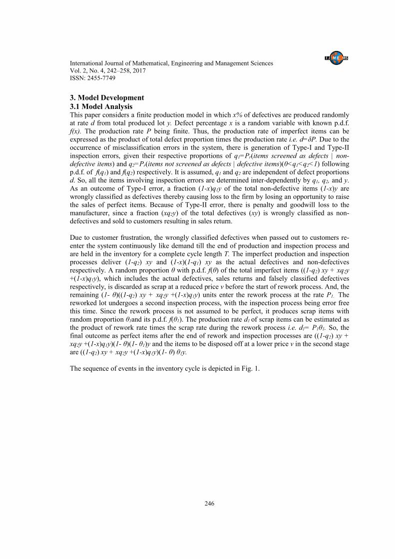
3. Model Development 3.1 Model Analysis This paper considers a finite production model in which x% of defectives are produced randomly at rate d from total produced lot y. Defect percentage x is a random variable with known p.d.f. f(x). The production rate P being finite. Thus, the production rate of imperfect items can be expressed as the product of total defect proportion times the production rate i.e. d=δP. Due to the occurrence of misclassification errors in the system, there is generation of Type-I and Type-II inspection errors, given their respective proportions of q1=Pr(items screened as defects | non- defective items) and q2=Pr(items not screened as defects | defective items)(0<q1<q2<1) following p.d.f. of f(q1) and f(q2) respectively. It is assumed, q1 and q2 are independent of defect proportions d. So, all the items involving inspection errors are determined inter-dependently by q1, q2, and y. As an outcome of Type-I error, a fraction (1-x)q1y of the total non-defective items (1-x)y are wrongly classified as defectives thereby causing loss to the firm by losing an opportunity to raise the sales of perfect items. Because of Type-II error, there is penalty and goodwill loss to the manufacturer, since a fraction (xq2y) of the total defectives (xy) is wrongly classified as non-defectives and sold to customers resulting in sales return. Due to customer frustration, the wrongly classified defectives when passed out to customers re-enter the system continuously like demand till the end of production and inspection process and are held in the inventory for a complete cycle length T. The imperfect production and inspection processes deliver (1-q2) xy and (1-x)(1-q1) xy as the actual defectives and non-defectives respectively. A random proportion θ with p.d.f. f(θ) of the total imperfect items ((1-q2) xy + xq2y +(1-x)q1y), which includes the actual defectives, sales returns and falsely classified defectives respectively, is discarded as scrap at a reduced price v before the start of rework process. And, the remaining (1- θ)((1-q2) xy + xq2y +(1-x)q1y) units enter the rework process at the rate P1. The reworked lot undergoes a second inspection process, with the inspection process being error free this time. Since the rework process is not assumed to be perfect, it produces scrap items with random proportion θ1and its p.d.f. f(θ1). The production rate d1 of scrap items can be estimated as the product of rework rate times the scrap rate during the rework process i.e. d1= P1θ1. So, the final outcome as perfect items after the end of rework and inspection processes are ((1-q2) xy + xq2y +(1-x)q1y)(1- θ)(1- θ1)y and the items to be disposed off at a lower price v in the second stage are ((1-q2) xy + xq2y +(1-x)q1y)(1- θ) θ1y. The sequence of events in the inventory cycle is depicted in Fig. 1.


247

y

Inspection

xy (1-x)y

(1-q2)xy xq2y (1- x) q1y (1- x) )(1-q1)y

SALES

Imperfect Proportion (x)

(1-q2) (1- q1) (q

2) (Type-II error)

Perfect Proportion (1- x)

Sales returns

(q1) (Type-I error)

Total Imperfect Items

[x+ q1 (1- x)] y = δy

(θ) Non-Reworkable (1-θ) Reworkable

yδθ yδ(1-θ)

Inspection

(1-θ1) Perfect

δ(1-θ) θ1y δ(1-θ)(1-θ)y

TOTAL SCRAP

(θ1) Scrap

Fig. 1. Sequence of events in the inventory cycle

3.2 Model Formulation In this segment, a mathematical model befitting the above exposed problem, assumptions and description has been formulated. The behavior of inventory cycle depicting the concerned situation is shown in Fig. 2.


248

Fig. 2. Inventory behaviors of (a) imperfect production and inspection system, (b) defective items sorted through inspection process, (c) total scrap items (d) sales returns


249

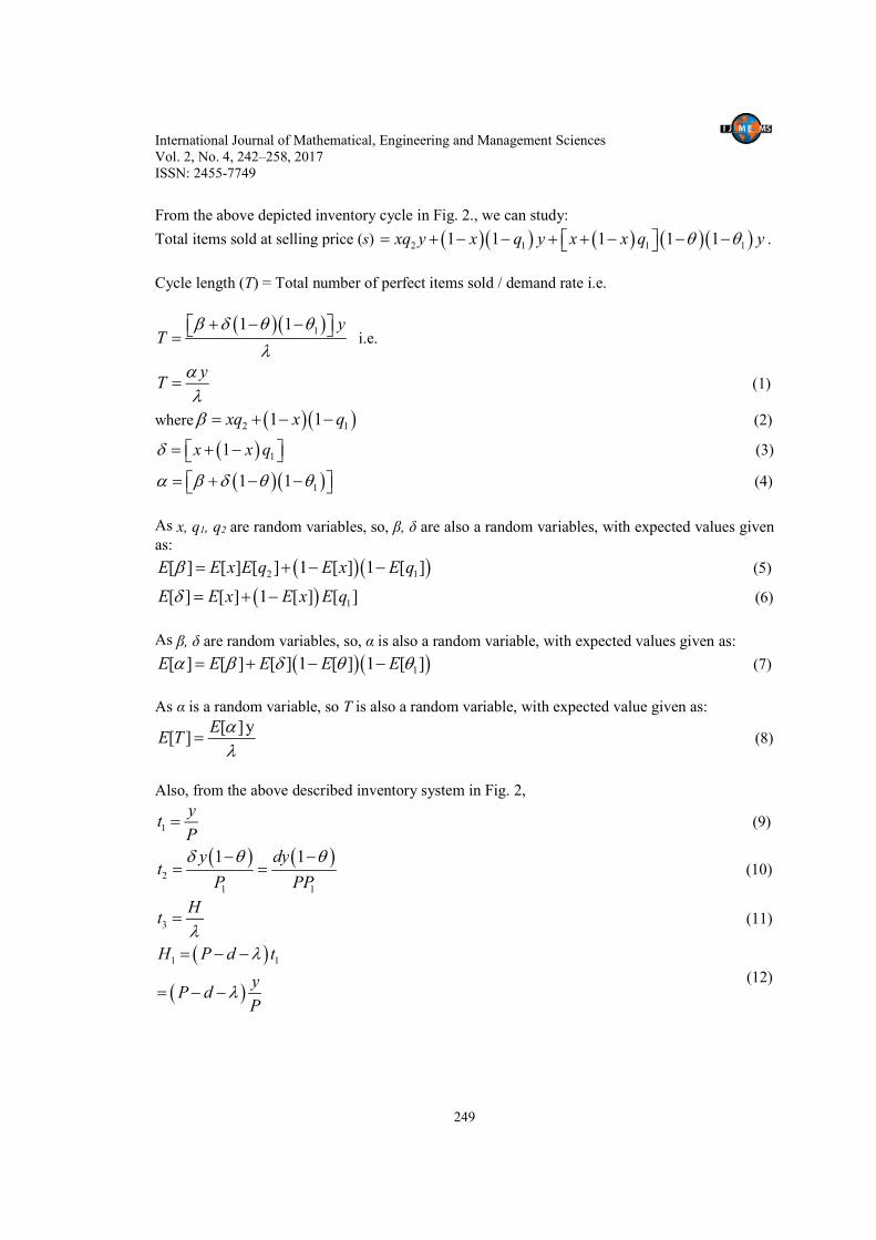
From the above depicted inventory cycle in Fig. 2., we can study:

Total items sold at selling price (s) 2 1 1 11 1 1 1 1xq y x q y x x q y .

Cycle length (T) = Total number of perfect items sold / demand rate i.e.

11 1 yT

i.e.

yT

(1)

where 2 11 1xq x q (2)

11x x q (3)

11 1 (4)

As x, q1, q2 are random variables, so, β, δ are also a random variables, with expected values given as:

2 1[ ] [ ] [ ] 1 [ ] 1 [ ]E E x E q E x E q (5)

1[ ] [ ] 1 [ ] [ ]E E x E x E q (6)

As β, δ are random variables, so, α is also a random variable, with expected values given as:

1[ ] [ ] [ ] 1 [ ] 1 [ ]E E E E E (7)

As α is a random variable, so T is also a random variable, with expected value given as:

[ ]y[ ]

EE T

(8)

Also, from the above described inventory system in Fig. 2,

1

yt

P (9)

2

1 1

1 1y dyt

P PP

(10)

3

Ht

(11)

1 1H P d t

yP d

P

(12)


250

1 1 1 2

1 1

1

1

H H P d t

dyyP d P d

P PP

(13)

3.2.1 Relevant Costs Various cost components taken into account are: (i) Production Cost, which includes fixed and variable procurement costs per cycle, i.e.,

PC K cy (14)

(ii) Inspection Cost, which includes the cost of inspection, i.e., IC=iy (15) (iii) Misclassification Error -1 Cost, which includes the cost of Type-I error. i.e.,

11 1rEC c x q y (16)

(iv) Misclassification Error -2 Cost which includes the cost of Type-II error. i.e.,

22 aEC c xq y (17)

(v) Rework Cost, which includes the cost of reworking of each defective item, i.e.,

1wRC c y (18)

(v) Disposal Cost, which includes the cost of disposing off each scrap item, i.e.

1 1DC u y (19)

(vi) Inventory Holding Cost is the cost of carrying all non-defectives, defectives, reworked and items returned from the market. From Fig. 2, it can be calculated as

1 2 31 1 1 2 1 21 1 2

2 2 2 2 2 2

H H t HtH t dt xq yT PtHC h t h t

(20)

Therefore, by using equations (14)-(20), total cost per cycle is given by:

Total cost (T.C.) = PC + IC + EC1+ EC2 + RC + DC + HC (21)


251

21 2 1 2

2 22 22 2 2

1 12 2 2 2 21 1 1

222 2 2 22

1 1 12 2 21 1

1 1 12

1 1 1

2 2 2

1 1

2 2 2 2

r a w

h P dK cy iy c x q y c xq y c y u y y

P

d d d h P dh P d y h P d y h P d y y

P P P P P P P

d dh xqhdh P d P d y y y h y

P P P P P

(22)

3.2.2. Sales Revenue The total sales revenue consists of four parts: (i) Sales from sorted perfect items is

1 2 11 1R s xq y x q y (23)

(ii) Revenue loss from Sales Return

2 2R sxq y (24)

(iii) Sales from reworked items

3 11 1R s y (25)

(iv) Sales from total scrap items

4 11R v y y (26)

Therefore, by using equations (23)-(26), total sales revenue per cycle is given by: Total Revenue (T.R.) = R1 + R2 + R3 +R4 (27)

2 1 2 1 11 1 1 1 1s xq y x q y sxq y s y v y y (28)

3.2.3 Manufacturer’s Total Profit For obtaining Total Profit (T.P.), we subtract equation (22) from (28) i.e.


252

2 1 2 1 1

21 2 1 2

2 22 22 2 2

1 12 2 2 2 21 1 1

1 1

. . 1 1 1 1 1

1 1 12

1 1 1

2 2 2

r a w

T P s xq y x q y sxq y s y v y y K cy iy

h P dc x q y c xq y c y u y y

P

d d d h P dh P d y h P d y h P d y y

P P P P P P P

h P d P d

222 2 2 22

12 2 21 1

1 1

2 2 2 2

d dxqdy h y h y h y

P P P P P

(29)

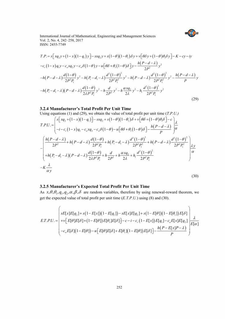
3.2.4 Manufacturer’s Total Profit Per Unit Time Using equations (1) and (29), we obtain the value of total profit per unit time (T.P.U.)

2 1 2 1 1

1 2 1

2 22 2

1 12 2 2 2 2 21 1 1

1 1

1 1 1 1 1

. . .1 1 1

1 1 1

2 2 2 2

1

2

r a w

s xq x q sxq s v c

T PU h P di c x q c xq c u

P

h P d d d dh P d h P d h P d

P P P P P P P

dh P d P d

P

22

212 2 2

1 1

1

2 2 2

y

dxqdh h h

P P P P

Ky

(30)

3.2.5 Manufacturer’s Expected Total Profit Per Unit Time

As 1 1 2, , , , , , ,x q q are random variables, therefore by using renewal-reward theorem, we

get the expected value of total profit per unit time (E.T.P.U.) using (8) and (30).

2 1 2 1

1 1 2

1

[ ] [ ] 1 [ ] 1 [ ] [ ] [ ] 1 [ ] 1 [ ] [ ]

. . . . [ ] [ ] 1 [ ] [ ] [ ] 1 [ ] [ ] [ ] [ ][ ]

[ ][ ] 1 [ ] [ ] [ ] [ ] 1 [ ] [ ]

r a

w

sE x E q s E x E q sE x E q s E E E

E T PU v E E E E E c i c E x E q c E x E qE

h P E x Pc E E u E E E E E

P


253

22 2

1 1 12 2 2 21 1

22 2

1 1 12 2 21 1

22 2

212 2

1

[ ] [ ] 1 [ ] [ ] 1 [ ][ ] [ ]

2 2 2

[ ] 1 [ ] [ ] 1 [ ][ ] [ ] [ ]

2 2

[ ] 1 [ ][ ] [ ] [ ][ ]

2 2 2

h P E x P E x P E E x P Eh P E x P h P E P

P P P P P

E x P E E x P Eh P E x P h P E P P E x P

P P P P

E x P EE E x E qE x Ph h h

P P P

[ ]

[ ]

y

E

KE y

(31)

4. Manufacturer’s Optimal Policy The manufacturer intends to maximize his expected total profit per unit time by optimizing the production quantity. In this section, concavity of the objective function is proved and a closed-form solution of the model is reached providing the required optimal production value to the manufacturer. The result is established in the form of a lemma. Lemma. The function of manufacturer’s expected total profit per unit time is concave. Proof. To prove the global concavity of the expected profit function, the following second-order sufficient condition of global optimality must hold:

Sufficient Condition: 2

2. . . . 0;

dE T PU

dy

By taking first order derivative of E.T.P.U. with respect to y, we obtain

2 21

2 22 2 2 2

1 1 1 2 2 2 21 1

21 1 1 2 2

1

2 2

1

[ ] [ ] 1 [ ][ ]

2 2

[ ] 1 [ ] [ ] 1 [ ][ ] [ ]

2 2. . . .

[ ] 1 [ ] [ ] [ ] [ ][ ][ ] [ ]

2 2 2

[ ] 1 [

h P E x P E x P Eh P E x P

P P P

E x P E E x P Eh P E P h P E x P

P P P PdE T PU

dy E x P E E E x E qE x Ph P E P P E x P h h

P P P

E x P Eh

2

21

2

[ ]

]

2

E

P P

K

E y

(32)

By taking second order derivative of E.T.P.U. with respect to y, we obtain


254

2

2 3

2. . . . 0

d KE T PU

dy E y

(33)

Hence, concavity of the objective function has been proved mathematically.

To determine the optimal value*y , which maximizes the function of E.T.P.U., the first-order

necessary condition of optimality must be satisfied:

Necessary Condition: . . . .

0d E T PU

dy .

On setting equation (31) equal to zero, we get:

*

22 2

1 1 12 2 2 21 1

22 2

1 1 12 2 21 1

22 2

212 2

1

[ ] [ ] 1 [ ] [ ] 1 [ ][ ] [ ]

2 2 2

[ ] 1 [ ] [ ] 1 [ ][ ] [ ] [ ]

2 2

[ ] 1 [ ][ ] [ ] [ ][ ]

2 2 2

Ky

h P E x P E x P E E x P Eh P E x P h P E P

P P P P P

E x P E E x P Eh P E x P h P E P P E x P

P P P P

E x P EE E x E qE x Ph h h

P P P

(34) which is the optimal values of y. Hence, Lemma is proved.

5. Numerical Analysis 5.1 Example This subsection validates the developed model with the help of a numerical. The optimal order quantity (y) and expected profit per unit time (E.T.P.U*) are determined for a given set of parameters. Let us consider a situation with the following parameters: Defect proportion (x), Proportion of Type-1 error (q1), Proportion of Type-2 error (q2), Proportion of non-reworkable items (θ), Proportion of failed reworked items (θ1) are assumed to follow Uniform distribution with their respective p.d.f. as:

25,0.05 0.11(x)

0,otherwise

xf

1

1

50,0.01 q 0.03(q )

0,otherwisef

2

2

50,0.01 q 0.03(q )

0,otherwisef

25,0.01 0.07( )

0,otherwisef

1

1

25,0.01 0.07( )

0,otherwisef

.

Using equations (5), (6) and (7), we obtain 0.9032E , 0.0984E , 0.9938E .


255

Other parameters are: P = 1,00,000 units/year, P1 = 80,000 units/year, λ = 50,000 units/ year, K = $ 250/ production, c =$ 30/ unit, s = $ 60/ unit, v = $ 20/ unit, u=$ 8 /unit-, i = $10/ unit, Ca= $ 12/ unit, Cr= $ 10/ unit, Cw= $ 15/ unit, h = $ 5/ unit, h1 = $ 8/ unit, x= 0.08, q1 = 0.02, q2 = 0.02, θ= 0.04, θ1 = 0.04.

From eq. (34), (31) and (1), the optimal production lot size* 725y units/ cycle, with

corresponding *. . . $4,18,507 / yearE T PU and * 7T days respectively.

Verification of no shortage condition: (1-x)P = 92000 > λ. So, there are no shortages in the model.

5.2 Sensitivity Analysis Variation in the values of parameters may happen due to uncertainties in any decision-making situations. To analyze these changes, sensitivity analysis has been performed to study the effect of changes in main parameters x, q1, q2, θ and θ1 on the optimal production and control variables y* and T.P.U.*. Results are summarized in Tables 1-5 using the data of above solved numerical. From the results shown in the Tables 1-5, we obtain the following managerial insights:

x y* T.C.U.* E.T.P.U.*

0.04 1,094 25,56,721 4,45,528

0.06 865 25,70,694 4,31,896

0.08 725 25,84,425 4,18,507

0.10 630 25,97,952 4,05,323

Table 1. Impact of x on optimal production policy

θ y* T.C.U.* E.T.P.U.*

0.02 716 25,80,574 4,20,455

0.04 725 25,84,425 4,18,507

0.06 735 25,88,289 4,16,553

0.08 745 25,92,166 4,14,593

Table 2. Impact of θ on optimal production policy

As visible in Table 1, with the increase in the proportion of defectives (x), the production quantity (y*) decreases along with the profit values (E.T.P.U.*). Therefore, it is beneficial for the manufacturer to reduce the percentage of defects by identifying the causes of imperfections as these have adverse effect on his sales and also reputation in the long run. From Table 2, it is evident that with the increase in the value of non-reworkable proportion (θ) of total accumulated defectives, there is decrease in the proportion (1-θ) i.e. the rework proportion. This means lesser items will be recovered after rework process reducing the maximum possible sales and hence the profit values (E.T.P.U.*). There is also increase in the production quantity (y*) since more units will be required to satisfy the demand with perfect items.


256

θ1 y* T.C.U.* E.T.P.U.*

0.02 725 25,78,768 4,22,261

0.04 725 25,84,425 4,18,507

0.06 725 25,90,104 4,14,738

0.08 725 25,95,804 4,10,955

Table 3. Impact of θ1 on optimal production policy

q1 y* T.C.U.* E.T.P.U.*

0.00 725 21,04,630 8,96,848

0.01 725 23,44,354 6,57,851

0.02 725 25,84,425 4,18,507

0.03 725 28,24,845 1,78,815

Table 4. Impact of q1 on optimal production policy

Table 3 reflects negative impact of higher value of scrap proportion (θ1) of reworked items on total profit (E.T.P.U.*) of the inventory system. Consequently, there is decrease in the proportion of perfectly repaired items (1-θ1) which cause reduction in the number of perfect items and hence decrease in value of (E.T.P.U.*). However, the there is no change in the production quantity (y*). As shown in Table 4, by committing more misclassification errors of Type-I (q1), the manufacturer is unable to sell all the perfect items as he is discarding some of them as scrap by mistake. Though a proportion of falsely classified defectives as non-defectives are recovered by rework process but the overall effect is the decrease in the value of (E.T.P.U.*).

q2 y* T.C.U.* T.P.U.*

0.00 725 25,80,527 4,27,247

0.01 725 25,82,478 4,22,873

0.02 725 25,84,425 4,18,507

0.03 725 25,86,370 4,14,147

Table 5. Impact of q2 on optimal production policy

It is observed from Table 5 that as the proportion of Type 2 error (q2) increases, there is increase in the units of sales returns since some defectives have been sold to customers by inspector’s mistake. Due to this misclassification, the manufacturer suffers penalty cost and goodwill losses. Though all the defect returns go through the rework process but only few are not recovered due to irreparable changes in some items and hence these are sold as scrap decreasing the value of (E.T.P.U.*).

6. Conclusion and Future Research In the present paper, a finite production model is developed to investigate the optimal production quantity by maximizing the expected total profit per unit time in an imperfect production, imperfect inspection and imperfect rework environment. In order to reduce the production-inventory costs significantly, it is beneficial for the manager to integrate a careful inspection


257

process to sort out the defectives from the produced lot. Despite the emergence of many sophisticated techniques, production of defectives is incontrovertible in most business firms. However, with little investment in the repair/rework methods, some of the defectives can be recovered and treated as perfect items after rework process. Since human errors are undeniable, the inspection team causes Type-I and Type-II errors during the inspection process. So, it is advisable for the manufacturer to identify the causes of errors to eliminate or reduce the defects. To be at par with today’s competitive market, one cannot overlook any chance to improve on quality, so, the concept of imperfect rework along with inspection errors has been incorporated to make the imperfect quality environment appear more relevant and applicable in practice. As per author’s knowledge, such a real life set-up has not been explored in the existing literature of inventory management. A numerical example along with a comprehensive sensitivity analysis is employed to demonstrate the practicality of the model. For future research, it would be interesting to extend the present model for different demand functions viz., stock dependent demand, price and time dependent demand or both. Another possible direction may be developed by incorporating different trade credit strategies in the present model. The model can also be studied under the effect shortages, deterioration, inflation, two warehousing etc.

References

Cárdenas-Barrón, L. E. (2009). Economic production quantity with rework process at a single-stage manufacturing system with planned backorders. Computers & Industrial Engineering, 57(3), 1105-1113.

Chiu, S. W. (2008). Production lot size problem with failure in repair and backlogging derived without derivatives. European Journal of Operational Research, 188(2), 610-615.

Chiu, S. W., Gong, D. C., & Wee, H. M. (2004). Effects of random defective rate and imperfect rework process on economic production quantity model. Japan Journal of Industrial and Applied Mathematics, 21(3), 375-389.

Chiu, S. W., Ting, C. K., & Chiu, Y. S. P. (2007). Optimal production lot sizing with rework, scrap rate, and service level constraint. Mathematical and Computer Modelling, 46(3), 535-549.

Chiu, Y. P. (2003). Determining the optimal lot size for the finite production model with random defective rate, the rework process, and backlogging. Engineering Optimization, 35(4), 427-437.

Chiu, Y. S. P., Lin, H. D., & Cheng, F. T. (2006). Optimal production lot sizing with backlogging, random defective rate, and rework derived without derivatives. Proceedings of the Institution of Mechanical Engineers, Part B: Journal of Engineering Manufacture, 220(9), 1559-1563.

Chung, K. J. (2011). The economic production quantity with rework process in supply chain management. Computers & Mathematics with Applications, 62(6), 2547-2550.

Duffuaa, S. O., & Khan, M. (2005). Impact of inspection errors on the performance measures of a general repeat inspection plan. International Journal of Production Research, 43(23), 4945-4967.

Hayek, P. A., & Salameh, M. K. (2001). Production lot sizing with the reworking of imperfect quality items produced. Production Planning & Control, 12(6), 584-590.

Hsu, J. T., & Hsu, L. F. (2013a). An EOQ model with imperfect quality items, inspection errors, shortage backordering, and sales returns. International Journal of Production Economics, 143(1), 162-170.

Hsu, J. T., & Hsu, L. F. (2013a). Two EPQ models with imperfect production processes, inspection errors, planned backorders, and sales returns. Computers & Industrial Engineering, 64(1), 389-402.


258

Hsu, J., & Hsu, L. (2014). A supplement to an EOQ model with imperfect quality items, inspection errors, shortage backordering, and sales return. International Journal of Industrial Engineering Computations, 5(2), 199-210.

Jaggi, C. K., Khanna, A., & Kishore, A. (2016, March). Production inventory policies for defective items with inspection errors, sales return, imperfect rework process and backorders. In K. Singh, M. Pandey, L. Solanki, S. B. Dandin, & P. S. Bhatnagar (Eds.), AIP Conference Proceedings (Vol. 1715, No. 1, p. 020062). AIP Publishing.

Jamal, A. M. M., Sarker, B. R., & Mondal, S. (2004). Optimal manufacturing batch size with rework process at a single-stage production system. Computers & Industrial Engineering, 47(1), 77-89.

Khan, M., Jaber, M. Y., & Bonney, M. (2011). An economic order quantity (EOQ) for items with imperfect quality and inspection errors. International Journal of Production Economics, 133(1), 113-118.

Konstantaras, I., Skouri, K., & Jaber, M. Y. (2012). Inventory models for imperfect quality items with shortages and learning in inspection. Applied Mathematical Modelling, 36(11), 5334-5343.

Lee, H. L., & Rosenblatt, M. J. (1987). Simultaneous determination of production cycle and inspection schedules in a production system. Management Science, 33(9), 1125-1136.

Liou, M. J., Tseng, S. T., & Lin, T. M. (1994). The effects of inspection errors to the imperfect EMQ model. IIE transactions, 26(2), 42-51.

Liu, N., Kim, Y., & Hwang, H. (2009). An optimal operating policy for the production system with rework. Computers & Industrial Engineering, 56(3), 874-887.

Makis, V. (1998). Optimal lot sizing and inspection policy for an EMQ model with imperfect inspections. Naval Research Logistics (NRL), 45(2), 165-186.

Porteus, E. L. (1986). Optimal lot sizing, process quality improvement and setup cost reduction. Operations Research, 34(1), 137-144.

Rezaei, J. (2016). Economic order quantity and sampling inspection plans for imperfect items. Computers & Industrial Engineering, 96(C), 1-7.

Rosenblatt, M. J., & Lee, H. L. (1986). Economic production cycles with imperfect production processes. IIE Transactions, 18(1), 48-55.

Salameh, M. K., & Jaber, M. Y. (2000). Economic production quantity model for items with imperfect quality. International Journal of Production Economics, 64(1), 59-64.

Sana, S. S. (2010a). A production–inventory model in an imperfect production process. European Journal of Operational Research, 200(2), 451-464.

Sana, S. S. (2010b). An economic production lot size model in an imperfect production system. European Journal of Operational Research, 201(1), 158-170.

Sana, S. S. (2011). A production-inventory model of imperfect quality products in a three-layer supply chain. Decision Support Systems, 50(2), 539-547.

Schrady D. A (1967). A deterministic inventory model for repairable items. Naval Research Logistics, 14(3), 391-398.

Taft, E. W. (1918). The most economical production lot. Iron Age, 101(18), 1410-1412.

Yoo, S. H., Kim, D., & Park, M. S. (2009). Economic production quantity model with imperfect-quality items, two-way imperfect inspection and sales return. International Journal of Production Economics, 121(1), 255-265.

Documents

Inventory Modeling for Imperfect Production Process …-no.-4,-242–258,-2017.pdfscrap items before the beginning of rework process and considered that a random proportion, with