Inventory Dynamics and Business Cycles:

What Has Changed?†

Jonathan McCarthy‡ Egon Zakrajsek§

June 2003

Abstract

Despite the recent patch of sluggish growth, the U.S. economy has experienced a pe-riod of remarkable stability since the mid-1980s. One popular explanation attributes thediminished variability of economic activity to information-technology led improvementsin inventory management. Our results, however, indicate that the changes in inven-tory dynamics since the mid-1980s played a reinforcing—rather than a leading—rolein the volatility reduction. Movements in the volatility of manufacturing output overthe past three decades almost entirely reflect changes in the variability of the growthcontribution of sales. Although the volatility of total inventory investment has fallen,the decline occurred well before the mid-1980s and was driven by the reduced variabilityof materials and supplies. Our analysis does show that since the mid-1980s inventorydynamics have played a role in stabilizing manufacturing production: Inventory “imbal-ances” tend to correct more rapidly, and the quicker response of inventories to monetarypolicy and commodity price shocks buffers production from fluctuations in sales to agreater extent. But more extensive production smoothing and faster dissolution of in-ventory imbalances appear to be a consequence of changes in the way industry-levelsales and aggregate economic activity respond to shocks, rather than a cause of changesin macroeconomic behavior.

JEL Classification: E32, E22, D24Keywords: inventories, inventory management, business cycles, GDP volatility

†We thank Doug Elmendorf, Michael Feroli, Mark Gertler, Kenneth Kuttner, Andrew Levin, Dan Sichel,Eric Swanson, Stacey Tevlin, Jonathan Wright, and participants of the New York Fed Domestic ResearchBrown Bag seminar and the Federal Reserve Board macro workshop for helpful comments. Amanda Coxprovided outstanding research assistance. The views expressed in this paper are solely the responsibility ofthe authors and should not be interpreted as reflecting the views of the Board of Governors of the FederalReserve System, the Federal Reserve Bank of New York, or of any other person associated with the FederalReserve System.‡Research Department, Federal Reserve Bank of New York, 33 Liberty Street, New York, NY, 10045.

Email: jonathan.mccarthy@ny.frb.org; Tel: (212) 720-5645.§Corresponding author: Division of Monetary Affairs, MS-84, Board of Governors of the Federal Reserve

System, 20th Street & Constitution Avenue, NW, Washington D.C., 20551. Email: egon.zakrajsek@frb.gov;Tel: (202) 728-5864.

1

1 Introduction

The economic stability of the 1983–2000 period stands out in marked contrast to the frequentand relatively severe cyclical fluctuations that characterized the American economy throughmuch of the twentieth century. Between 1983 and 2000, the U.S. experienced two of thelongest economic expansions and one of the mildest and shortest recessions on record. Whilethe economic downturn in 2001 and the subsequent wobbly recovery have shown that thebusiness cycle is far from dead, the striking decrease in the volatility of real aggregate outputsince the mid-1980s continues to intrigue researchers.1

Economists have advanced a number of explanations for the decline in the volatility ofaggregate output; see Stock and Watson (2002) for a comprehensive review. Among theleading hypotheses is that more transparent and credible monetary policy since the “Volckerdeflation” of the early 1980s has resulted in a more stable economic environment. A second,“good luck,” theory argues that economic shocks (e.g., productivity and commodity priceshocks) have been milder over the past twenty years. A third hypothesis, which has receiveda great deal of attention, points to the widespread adoption of better business practices—in particular, inventory management techniques—spurred by technological advances of thepast two decades.2

In this paper, we focus principally on the better business practices hypothesis, or whatwe call the inventory conjecture. Proponents of this view argue that while the concept of in-tegrated physical distribution management has been around since the 1960s, advances in in-formation technology over the past two decades have only just recently made its widespreadimplementation possible.3 As a result, firms are now better able to control production anddelivery processes, and thus identify and resolve inventory imbalances more rapidly. Be-cause enterprises now operate on the basis of essentially the same information set, economicdecisions of firms within and across industries may have become more synchronized. Inthe aggregate, synchronous efforts to correct emerging inventory imbalances may induce

1McConnell and Perez-Quiros (2000) provided the first rigorous evidence of a decline in real GDP volatil-ity, which their statistical techniques placed in the first quarter of 1984. Subsequently, a number of studiesemploying different statistical methods confirmed that real GDP has become more stable since the mid-1980s;see, for example, Kim, Nelson, and Piger (2001), Ahmed, Levin, and Wilson (2001), Sensier and van Dijk(2001), Blanchard and Simon (2001), and Stock and Watson (2002). Unlike McConnell and Perez-Quiros(2000), however, these studies found that the decline in GDP volatility is emblematic of reduced volatilityin many economic series, both real and nominal, over the past two decades.

2Other possible factors such as changes in data construction, a shift in the composition of output fromgoods toward services, and changes in fiscal policy appear to have played relatively unimportant roles in thestep-down of volatility since the mid-1980s.

3Integrated physical distribution management is a total system approach to the management of inter-related activities such as transportation, warehousing, order processing, inventory/production scheduling,and consumer service. According to a survey of firms in the late 1970s by Lambert and Mentzer (1978), thelack of necessary cost data—in particular, inventory carrying costs at different stages of production—hadseriously hampered a full, successful implementation of this system.

2

a steeper initial contraction in economic activity, but because these imbalances are morereadily contained, they are less persistent and inventory runoffs—and consequently businesscycles—thus should be less severe.

Efforts by economists to attribute the reduction in the volatility of aggregate eco-nomic activity to improvements in inventory management—or to any other source for thatpurpose—are and will remain controversial. This is so because the step-down in volatil-ity since the mid-1980s constitutes essentially a single episode in the evolution of the U.S.economy. Consequently, it is difficult to disentangle causal explanations from ones that arecorrelated with the reduction in volatility merely because of a coincidence of timing. Theinventory conjecture is especially susceptible to this criticism, as it abounds with anecdotalevidence and case studies linking the information revolution with the use of this technologyby firms to manage more efficiently their production and inventories.

Formal statistical evidence on the issue is also largely indirect. McConnell and Perez-Quiros (2000) (MPQ hereafter), for example, trace the GDP volatility reduction to a narrowsource—a structural break in the volatility of durable goods output. Because they do notfind a similar decline in the variability of final sales of durable goods, MPQ argue that a morestable economy since the mid-1980s stems from a reduction in the volatility of inventoryinvestment in that sector. Moreover, they argue, the timing of the break in the volatility ofdurable goods output occurs after the widespread adoption of just-in-time (JIT) techniquesand computerized production and supply-chain management by U.S. manufacturers duringthe late 1970s and early 1980s.4 The effects of these innovations are evident in the declinein the aggregate inventory-sales ratio, as firms are able to meet production and sales withleaner stocks, and in a significant reduction in the time between ordering and receivingparts and other production materials (see McConnell, Mosser, and Perez-Quiros (1999)).

Earlier attempts to assess more directly the effects of changes in inventory control meth-ods on the business cycle by Morgan (1991), Bechter and Stanley (1992), Little (1992), Allen(1995), and Filardo (1995) have reached mixed conclusions. These authors agree that theadoption of new inventory management techniques has resulted in a lower ratio of invento-ries to sales, but the impact of these innovations on cyclical fluctuations, at least throughthe mid-1990s, is ambiguous.

More recently, Kahn, McConnell, and Perez-Quiros (2001) developed a theoretical modelincorporating both inventories and information technology. In their model, advances in

4Pioneered by the Japanese, JIT management of production allows firms to keep a minimum of inventoriesof work-in-progress, raw materials, parts, and other supplies, thereby lowering inventory financing costs.Because JIT delivery methods respond mostly to the current conditions on the factory’s floor, they workbest when demand is predictable. JIT practices, however, can be combined with the computer-drivensystems that initiate production and place orders in anticipation of future demand. Because businesses haveto purchase the necessary computer systems and train workers to use them, this technology is expensiverelative to JIT; see Little (1992) for additional details.

3

information technology improve information about final demand and thus lead to a lowerratio of inventories to sales and diminished output variability. Their simulation results,however, suggest that the quantitative effects of better information on the variability ofinventory investment and, consequently, output are modest.

Following a different tack, Feroli (2002) calibrates a variant of the neoclassical growthmodel in which inventories enter the production function along with labor, nonresidentialstructures, and equipment and software (E&S). The key finding is that the sustained fall ofE&S prices relative to the price of inventories has caused firms to substitute E&S for inven-tory stocks, thus inducing a decline in the aggregate inventory-sales ratio.5 The technicalsubstitution of capital equipment for inventory stocks, however, has a negligible effect onthe volatility of output.

In a recent study, Irvine and Schuh (2003), using an accounting framework and industry-level data, attribute about one-half of the decline in gross output volatility since the mid-1980s to lessened variability of inventory investment in both the manufacturing and tradesectors; the remaining one-half can be accounted for by the diminished comovement ofsales between industries. Although they do not directly examine the inventory adjustmentprocess nor the interaction between aggregate shocks and industry-level inventory dynamics,they interpret their results as reflecting a growing sophistication of supply and distributionchains among firms and across industries.

With the issue far from resolved and intriguing evidence abounding, we investigate theinventory conjecture utilizing disaggregated (by industry and stage of fabrication), high-frequency data. Our empirical strategy consists of two parts. To determine more accuratelythe changes in the volatility of manufacturing activity, as well as to compare the timing ofthese changes with the decline in the variability of aggregate output, we first examine theevolution of the volatility of production, shipments, and inventories at the broad sectorallevel. In the second part, we assess whether changes in industry-level inventory adjust-ment since the mid-1980s have stabilized production to a greater extent than previously, assuggested by the inventory conjecture.

Our decomposition of the unconditional variance of the growth rate of manufacturingoutput indicates that the observed decline in production volatility in that sector since themid-1980s stems overwhelmingly from a reduction in the volatility of shipments rather thanthe volatility of finished goods inventory investment. Next, we parse the variance of totalinventory investment and find that it has been trending lower since the mid-1970s, drivenlargely by a substantial decrease in the volatility of its materials and supplies component.The timing of the decline in the variance of inventory investment in materials and supplies is

5As noted by Feroli (2002), this explanation is consistent with the inventory conjecture, which holds thatthe reduction in average inventory holdings over the past two decades is a direct result of firms utilizingcheaper information processing equipment and software.

4

consistent with the adoption of JIT and other inventory management innovations in responseto the oil price shocks of the 1970s. However, there appears to be little systematic reductionin the unconditional variance of inventory investment at other stages of fabrication.

In the second part of the paper, we employ two empirical models to study the changesin inventory adjustment since the mid-1980s. The first model, a vector autoregression,links industry shipments, relative prices, and inventories at different stages of productionto a model typically used to identify the effects of monetary policy and other shocks onaggregate economic activity. In addition, we estimate industry-level inventory adjustmentspeeds at different stages of fabrication, using a version of the accelerator model with time-varying targets. We find that industry-level responses of inventories to monetary policy andsupply shocks since the mid-1980s are consistent with firms buffering production from salesfluctuations to a greater extent than in the earlier period. Our estimates of adjustmentspeeds also indicate a significantly faster dissipation of inventory imbalances since the mid-1980s, especially for finished goods and work-in-progress stocks.

The prevalence of production smoothing and faster inventory adjustment in the laterperiod, however, appears to be driven largely by changes in the way aggregate economicactivity and industry shipments respond to aggregate shocks. We thus interpret our resultsas suggesting that changes in the macroeconomic environment—most likely a shift to a moretransparent and less activist monetary policy—were likely the key factors in the moderationof output volatility. Improvements in inventory control methods, however, appear to haveamplified the reduction in output volatility.

2 Data

Throughout our analysis, we use monthly, industry-level (2-digit SIC) data for the manu-facturing sector provided by the Bureau of Economic Analysis (BEA).6 Our key variablesfor the twenty manufacturing industries—sales, materials and supplies inventories, work-in-progress inventories, and finished goods inventories—are seasonally adjusted and reportedin millions of chain-weighted 1996 dollars. Inventory stocks are measured as of the end-of-period, and sales are defined as the value of shipments. The sample covers the period fromJanuary 1967 through December 2000, yielding a balanced panel of 408 monthly observa-tions per industry, for a total of 8,160 industry/month observations.

Although the manufacturing sector accounts for a relatively small (and declining) share6In spring 2001, the BEA and the Census Bureau, the BEA’s source of the raw book-value of inventories

used to calculate real inventory stocks, replaced the SIC system with the North American Industrial Clas-sification System (NAICS). At the time of this paper, NAICS-classified data were available only startingin the early 1990s. For this reason, as well as to make the paper comparable to earlier studies, we useindustry-level data aggregated according to the SIC system. The twenty manufacturing industries, alongwith their respective 2-digit SIC codes, are listed in the Appendix.

5

of aggregate economic output (26.5 percent of GDP in 1967 and 15.9 percent in 2000), itsshare of goods production is more substantial. Manufacturing firms accounted for morethan 80 percent of durable goods GDP in the late 1960s, and even though this share hasfallen over the years, they still accounted for more than 50 percent of durable goods GDPin 2000. In the nondurable goods sector, by contrast, the manufacturing share of GDP hasremained fairly steady at about 35 percent over this period.

At the beginning of our sample period, U.S. manufacturers also held more than 50percent of aggregate inventory stocks, but this share has fallen to about 35 percent in2000. By sector, the manufacturing share of durable goods inventories has declined from60 percent in the late 1960s to about 40 percent by the end of 2000; for nondurable goods,the manufacturing share has decreased from 40 percent to about 25 percent over the sameperiod. Despite the diminished role of manufacturing firms in overall economic activity,their still-sizable presence in goods production, along with the fact that the factory sectorwas an early adopter of inventory and production control innovations, warrants our narrowfocus.

3 Evolution of Volatility

In this section, we establish some facts about the variability of manufacturing production,sales, and inventories at the sectoral level. This provides a more direct comparison tothe previous research documenting the decline in the volatility of similar, though typicallybroader, components of GDP. We begin by parsing out changes in the variance of sectoraloutput to changes in the variance of sales and inventory investment as well as to changes intheir covariance. We then turn to the evolution of volatility of total inventory investmentand of inventory investment at each stage of fabrication.

3.1 Methodology

Because our data are chain-weighted, the components of an aggregate are not additive(see Whelan (2000)). The growth contributions of components, however, do add up to thegrowth rate of the chain-weighted aggregate. In addition, because the growth contributionof a component is approximately equal to its share of the nominal aggregate times thecomponent’s growth rate, working with growth contributions adjusts for the fact that avery volatile component may have little effect on the overall volatility if it accounts for asmall share of the aggregate. Accordingly, we decompose the growth rate of output andtotal inventories into the growth contributions of their respective components. In particular,

6

we write the growth rate of a generic aggregate Xt in period t, denoted by %∆Xt, as

%∆Xt =∑j

gjt , (3.1.1)

where gjt is the growth contribution of component j in period t.As in Blanchard and Simon (2001), our measure of the time-varying volatility of the

growth contribution gjt is a rolling unconditional sample standard deviation. We use athree-year (36-month) window to compute these standard deviations, with rates of changeexpressed at a monthly basis. Because the monthly disaggregated data are volatile, we em-ploy a robust estimator of scale proposed by Rousseeuw and Croux (1993a) to mitigate theeffect of outliers.7 The comovements between growth contributions over time are measuredby rolling correlations, again computed over a 36-month window. To minimize the effect ofoutliers, we report 5-percent trimmed correlations, computed using the standardized sumsand differences method (see Huber (1981)).

3.2 Volatility of Output

Our starting point is the standard NIPA accounting identity

Qit ≡ Sit + ∆Hit, (3.2.1)

where Qit denotes real (gross) output or production of sector (industry) i in period t, Sitare real sales, and Hit are real finished goods inventory stocks at the end of period t.8 Using(3.2.1), we decompose the growth rate of output into the growth contribution of sales gSitand the growth contribution of finished goods inventory investment g∆H

it :

%∆Qit = gSit + g∆Hit .

7In particular, we use the Qn estimator with a small-sample correction factor derived in Rousseeuw andCroux (1993b). This estimator has a 50 percent breakdown point, is suitable for asymmetric distributions,and attains very high efficiency for Gaussian distributions. In addition, we examined the evolution ofvolatility of our key series using a GARCH model. The contours in the conditional variance of output, sales,and inventory investment from a GARCH specification match up closely with those of the unconditionalvolatility reported in the paper.

8Although we define output using identity (3.2.1), we construct real output by calculating a proper chain-aggregated output index; see Whelan (2000) for details. An additional issue concerning construction of anoutput measure is whether to include work-in-progress inventories in the inventory investment term ∆Hit.According to Blinder (1986), including work-in-progress inventories may provide a more accurate economicmeasure of output, though restricting inventory investment to finished goods is more standard in empiricalwork on inventory dynamics. We performed our analysis using both measures of output, and our resultswere virtually identical, as the correlation between the growth rates of the output measures is 0.94 for thedurable goods and 0.98 for the nondurable goods sector.

7

The growth contributions are calculated in a manner consistent with chain aggregation usedin the NIPA and thus are well-defined for both positive and negative values of ∆Hit.

The variance of the growth rate of real output for sector i is then given by

Var(%∆Qit) = Var(gSit) + Var(g∆Hit ) + 2× Cov(gSit, g

∆Hit ). (3.2.2)

The paths of the standard deviations corresponding to the variance terms in (3.2.2) arepresented in Figure 1. To provide a reference for possible volatility breaks, thin verticallines labeled 1984:Q1 and 1986:Q3 mark the break dates in the volatility of durable andnondurable goods GDP, respectively, as estimated by Kim, Nelson, and Piger (2001) (KNPhereafter).9 Shaded vertical bars denote NBER-dated recessions.

Surprisingly, neither sector of U.S. manufacturing appears to have experienced a markeddecline in output growth volatility (the solid line) around their respective KNP break dates.In the durable goods sector (upper panel), output volatility is somewhat lower after thebreak date, though it does not decline decisively until the mid-1990s. In the nondurablegoods sector (lower panel), output volatility begins to trend lower in the early 1980s, even-tually touching a historically low level during the late 1990s.10

Another notable feature in Figure 1 is that the evolution of the volatility of the growthcontribution of sales (dotted line) is strikingly similar to that of output volatility.11 Thevariability of the growth contribution of finished goods inventory investment (dashed line),by contrast, has remained in a narrow range throughout our sample period, and its move-ments are not well correlated with the swings in the volatility of output growth. Bothof these observations do not offer much support to the idea that widespread changes inproduction and inventory management in the mid-1980s resulted in more stable economicenvironment.

According to (3.2.2), however, inventory investment could have still contributed to alower output growth variance through changes in the sign or magnitude of the covari-ance between the growth contributions of inventory investment and sales. However, in thedurable goods sector, the movement in the correlation between the growth contributionsof inventory investment and sales shows no clear pattern, and its magnitude is generallymodest (Figure 2, upper panel). In the nondurable goods sector (lower panel), by contrast,this correlation has declined steadily during the past two decades, falling to about −0.6 by

9Ahmed, Levin, and Wilson (2001) and Stock and Watson (2002) find similar dates using differentmethods.

10We also performed this analysis using the Federal Reserve Board’s index of industrial production asan alternative measure of manufacturing output. In both sectors, the trends in output volatility using theindustrial production index are quite similar to those shown in Figure 1.

11This finding is consistent with the results reported by Ramey and Vine (2001), who show that salesshocks in the U.S. automobile industry during the 1990s have been far more transitory than during the1970s.

8

the end of the 1990s.12 Although this would suggest that production smoothing may havebecome more prevalent in the nondurable goods sector, the driving force of the reductionin the volatility of production, according to Figure 1, was still the decline in the variabilityof sales. Overall then, Figures 1–2 suggest that even though the volatility of GDP declinedmarkedly after the mid-1980s, there is little evidence that the timing coincides with thestabilization of manufacturing production and inventory investment.

3.3 Volatility of Inventories

According to the NIPA, it is total inventory investment rather than finished goods inventoryinvestment that enters into the measurement of GDP. In manufacturing, total inventories(Iit) consist of inventories of materials and supplies (Mit), work-in-progress (Wit), andfinished goods (Hit). It is quite plausible that improved management of inventories atearlier stages of fabrication is responsible for the diminished volatility of aggregate output.Using (3.1.1), the growth of total inventories, %∆Iit, can then be written as

%∆Iit = gMit + gWit + gHit , (3.3.1)

where gMit is the growth contribution of materials and supplies, gWit is the growth contri-bution of work-in-progress inventories, and gHit is the growth contribution of finished goodsinventories. We can then parse the variance of %∆Iit into the variances of its growth contri-butions and the covariances between growth contributions at different stages of fabrication.

The results of this exercise are summarized in Figures 3–5. The top panel of Figure 3ashows the evolution of the standard deviation of the growth rate of total inventories in thedurable goods sector, while the bottom panel depicts the paths of the volatilities of growthcontributions by stage of production. The same information for the nondurable goods sectoris presented in Figure 3b. To gauge the relative importance of inventories at different stagesof fabrication, we plot a rolling 36-month average share of each type of inventory in Figure 4.Comovements between growth contributions in (3.3.1) are shown in Figure 5.

As seen in the top panels of Figures 3a and 3b, the volatility of the growth rate of totalinventories in both the durable and nondurable goods sectors spiked in the aftermath of thefirst oil shock in 1973, the economic turmoil of the 1980-83 period, and the 1990-91 recession.These jumps in volatility are not surprising, given the well-documented role of inventoryinvestment during cyclical retrenchments; see, for example, Ramey and West (1999). Moststriking in both panels, however, is the inverted V-pattern of the standard deviation of total

12Blanchard and Simon (2001) report a similar change in the covariance between inventories and sales usingdata for the broader nonfarm business sector. Irvine and Schuh (2003) also find widespread evidence of thechange in the comovement between sales and inventory investment after the mid-1980s among manufacturingand trade industries.

9

inventory investment straddling KNP’s estimated dates of volatility reduction, a patternthat obscures the reduction in inventory investment volatility that began in the late 1970s.

The decrease in the standard deviation of total inventory growth during the late 1970scoincides with a decline in the volatility of the growth contribution of materials and supplies(Figures 3a and 3b, bottom panels). The reduction in the volatility of materials and supplies(dashed line) had begun in the mid-1970s, around the time when U.S. manufacturers startedto adopt JIT methods to reduce lead times and to better manage supply channels in the wakeof the first oil crisis. At the same time, there were modest declines in the volatility of thegrowth contribution of finished goods inventories. The volatility of the growth contributionof work-in-progress inventories, by contrast, displayed no discernible trend.

These patterns suggest that firms’ efforts during the late 1970s to stabilize inventory fluc-tuations were largely concentrated on their holdings of materials and supplies. Still, becausewe are working with growth contributions, it is possible that changes in the compositionof inventories have masked a decline in the volatility of other inventory components. Asshown in Figure 4, however, the shares of inventories at different stages of fabrication haveremained fairly constant over most of our sample period. The largest compositional shiftoccurred in the early 1990s among durable good producers (top panel), who over the courseof the decade significantly reduced the portion of inventories held as work-in-progress.13

The last set of factors that could account for the movements in the volatility of totalinventory investment are the correlations between the growth contributions of inventories atdifferent stages of fabrication (Figure 5). Most notably, these correlations moved largely intandem in the durable goods sector during most of the 1980s (top panel), which contributedto the inverted V-pattern of inventory investment volatility discussed earlier. In addition,the negative comovement of these factors in the late 1990s counteracted a runup in thestandard deviation of the growth contribution of finished goods inventories (see Figure 3a,bottom panel). In the nondurable goods sector, by contrast, correlations between thegrowth contributions of inventories at different stages of fabrication show no systematicpattern throughout the sample period (Figure 5, bottom panel).

In sum, the volatility patterns of production and inventory investment in manufacturingdo not change dramatically in the mid-1980s as suggested by the inventory conjecture.Rather, the volatility of output in the nondurable goods sector started to trend lower asearly as the mid-1970s, whereas in the durable goods sector, the most significant reduction inoutput volatility occurred during the early 1990s. More importantly, the reduction in outputvolatility in the factory sector is closely associated with a decrease in the variability of sales.Although total inventory investment has become less volatile, the decline in the standard

13Although the exact timing differs across durable goods industries, the fraction of inventories designatedas work-in-progress generally declined after the 1990–91 recession. The reductions are especially notable inthe large industries, SICs 35–38.

10

deviation of the growth rate of total inventories was driven primarily by a steady reductionin the volatility of its materials and supplies component that started in the aftermath of oilprice shocks of the 1970s.

4 Inventory Adjustment

So far, we have examined the volatility of manufacturing production and inventory invest-ment in isolation from the rest of the economy. However, manufacturing inventory behaviormay have changed in a manner consistent with the inventory conjecture, but the changein inventory dynamics as part of a business cycle propagation mechanism may have beena result of developments in the rest of the economy. We therefore next examine changesin the inventory adjustment process, while controlling for changes in the macroeconomicenvironment.

Our approach is twofold. First, we use a vector autoregression (VAR) model to exam-ine changes in the adjustment of inventories following aggregate shocks. The multivariateframework allows us to identify some linkages implicit in the inventory conjecture and totrack how responses of inventories at the industry level to common shocks may have changed.Second, we estimate industry-specific error-correction models for inventory investment ateach stage of fabrication. This approach provides a more direct method to assess changesin the inventory adjustment process, because the error-correction parameter measures thespeed with which inventories move toward their target level.

4.1 Inventory Adjustment and Aggregate Shocks

We begin by examining changes in the industry-level impulse response functions follow-ing monetary policy and aggregate supply shocks. The key feature of our specificationand identification scheme is that the VAR equations can be separated into two exogenousblocks—industry and aggregate.14 The industry block interlinks the dynamics of industrysales, relative output price, and inventories given the behavior of the aggregate variables.The aggregate block is a version of the Bernanke and Gertler (1995) model used to identifythe effects of monetary policy and other shocks on aggregate economic activity.

In assuming block-exogeneity, we impose the restriction that the industry-level variablesdo not enter into the aggregate block, whereas the aggregate variables enter into the industry

14Barth and Ramey (2001) use a similar block-exogenous VAR in their study of the “cost channel” ofmonetary transmission mechanism.

11

block. In particular, the reduced form of the VAR for industry i is given by[xityt

]= Ai(L)

[xit−1

yt−1

]+

[eitut

]; i = 1, 2, . . . , N, (4.1.1)

where xit = (sit pitmit hit)> is a vector of industry-specific variables consisting of (in loga-rithms) sales sit, relative output price pit, materials and supplies inventories mit, and thesum of work-in-progress and finished goods inventories hit. The output price in industry iis measured relative to the PCE price deflator, our aggregate price measure.

The aggregate block is described by the vector yt = (et pt pct rt)> comprising the loga-

rithm of a measure of aggregate economic activity et, the logarithm of the aggregate pricelevel pt, the logarithm of a commodity price index pct , and the effective Federal funds interestrate rt. Because we use monthly data, GDP is not readily available as a measure of aggre-gate economic activity. As an alternative, we use private nonfarm payroll employment.15

The commodity price index is the Journal of Commerce-Economic Cycle Research InstituteIndustrial Price Index.

Given our block-exogeneity assumption, the (8× 8) industry-specific matrix polynomialin the lag operator L in (4.1.1) takes the following form:

Ai(L) =

[Ai,11(L) Ai,12(L)

0 A22(L)

].

The (4 × 4) submatrix of zeros in the lower left corner encompasses the assumption thatlagged values of the industry variables do not affect the dynamics of the aggregate variables.

To identify the structural shocks underlying the reduced-form VAR innovations, weplace restrictions on the contemporaneous relationships between the variables. The firstset of restrictions comes from the block exogeneity assumption—industry variables haveno contemporaneous effect on the aggregate variables. The second is that the aggregatestructural shocks are identified, as in Bernanke and Gertler (1995), by a recursive orderingof private employment, price level, commodity prices, and the Fed funds rate. The third isthat aggregate variables affect some industry variables contemporaneously, which allows fora degree of strategic complementarity.16 In particular, the level of aggregate employmentmay affect industry output and price; the aggregate price level may influence industry-

15According to Warnock and Warnock (2000), volatility in aggregate employment has also fallen sincethe mid-1980s. To explore the robustness of our results to the choice of the aggregate activity variable, wealso performed the VAR analysis using the index of industrial production and real personal consumptionexpenditures in place of private employment. The substantive conclusions were the same as those presentedin the text.

16See Cooper and John (1988) and Blanchard and Kiyotaki (1987) for macro models containing suchcomplementarities.

12

level prices; and commodity prices may affect the inventory of materials and supplies.The fourth assumption is that industry sales and relative prices may affect inventoriescontemporaneously, but not vice versa. This assumption reflects the stickiness of price andproduction plans that underlie many New Keynesian models and seems reasonable giventhe monthly frequency of our data. The last assumption is that inventories at each stage offabrication are determined contemporaneously.

Under these restrictions, the relationship between the VAR innovations and structuralshocks can be written as:

Ai0

[eitut

]=

[εit

νt

];

[εit

νt

]∼ MVN(0,Σi), i = 1, 2, . . . , N,

where Σi is a diagonal covariance matrix of structural shocks, and

Ai0 =

1 0 0 0 ai,15 0 0 0ai,21 1 0 0 ai,25 ai,26 0 0ai,31 ai,32 1 ai,34 0 0 ai,37 0ai,41 ai,42 ai,43 1 ai,45 0 0 0

0 0 0 0 1 0 0 00 0 0 0 a65 1 0 00 0 0 0 a75 a76 1 00 0 0 0 a85 a86 a87 1

.

One issue in estimating the VAR is whether or not to remove trends from the series.Changes in the inventory-sales ratios owing to the adoption of new management techniqueshave certainly altered the relationship between inventories and sales at low frequencies,which may obscure changes in inventory dynamics at business cycle or higher frequencies.Accordingly, we used a one-sided exponential smoother with a gain parameter of 0.25 toremove a stochastic trend from each of our series; see, for example, Gourieroux and Monfort(1997). An attractive feature of this detrending procedure is that it preserves high-frequencytemporal patterns that may be distorted by two-sided filters such as the Hodrick-Prescottand Baxter-King band-pass filters.17 Given the high dimensionality of our system, anotherissue is parameter parsimony. To conserve degrees of freedom, we impose an asymmetriclag structure on our model—seven lags on the variables in the aggregate block and four lagson the variables in the industry block.18

17As a robustness check, we tried several other values for the gain parameter in the typical range between0.15 and 0.30, with negligible effects on our result. We also estimated the VAR in log levels. At shorterhorizons, the focus of our analysis, the pattern of impulse responses for employment, sales, and inventorieswas substantively similar to those we present in the paper.

18As suggested by Kilian (2001) and Ivanov and Kilian (2001), we determined the lag structure using the

13

The block-exogeneity assumption implies that the reduced-form specification (4.1.1)can be estimated industry by industry.19 Although the model is not recursive, standardlikelihood techniques can then be used to estimate the structural parameters in Ai,0 and Σi

for each industry (see Hamilton (1994), p. 330–33). Because of the volatility of the Fed fundsrate associated with the Volcker monetarist experiment, we exclude the 1979–83 period fromthe estimation. In addition, omitting the period associated with exceptional volatility andrestructuring in the manufacturing sector should enhance our ability to detect differencesin inventory dynamics across the subsamples. We thus estimate the structural parametersover two periods—1967:I–1978:XII and 1984:I–2000:XII—and compute the orthogonalizedimpulse responses. Using the industry-specific average shares of sales and inventories withineach sample period, we then aggregate industry responses to the sectoral level.

4.1.1 Responses to Monetary Policy Shocks

In this section, we examine the responses to a 50-basis-point shock in the Fed funds rateequation, commonly identified as a contractionary monetary policy shock. Figure 6a depictsimpulse responses for the aggregate block. Figures 6b and 6c contain impulse responses forthe durable and nondurable goods sectors, respectively; in addition to the impulse responsesof the four variables in the industry block, the two figures also depict the response of the loginventory-sales ratio for both materials and supplies and finished goods stocks, constructedas the difference between the responses of the log-level of inventories and the log-level ofsales.

Aggregate block: According to Figure 6a, the behavior of the employment in the earlyperiod (1967:I–1978:XII) displays the familiar response of aggregate economic activity toan unanticipated monetary policy tightening, as discussed, for example, by Bernanke andGertler (1995). Employment, relative to trend, does not begin to decline until about sixmonths after the policy tightening, but the response is persistent thereafter, with privateemployment running below trend up to 36 months after the initial shock. The response ofemployment in the later period (1984:I–2000:XII), by contrast, is quite different. Employ-ment falls below trend much more quickly, with the trough occurring six to nine monthsafter the unanticipated monetary policy tightening. Moreover, the response is considerablyless persistent, dying out within two years after the shock. These differences in the employ-ment responses will have a substantial effect on the dynamics of industry-level sales and

Akaike Information Criterion, allowing for some additional lags to preclude underfitting. We examined anumber of symmetric and asymmetric lag structures, and the substantive conclusions are very similar tothose presented in the paper.

19SIC 21 (Tobacco & Related Products) is omitted from the analysis because of suspect data.

14

inventories, even though the response of the Fed funds rate, at shorter horizons, is quitesimilar across the two periods.

Industry block: In the durable goods sector, there is a noticeable difference in the re-sponses of sales between the two periods (Figure 6b). The response of sales in the earlierperiod, like that of aggregate employment, is one typically expected after a contractionarymonetary policy shock: After a delayed decline, sales are persistently below trend for morethan two years. The response of sales in the post-1983 period, again much like that of theaggregate activity, is quicker, larger, but less persistent. Sales bottom out about six monthsafter the shock—roughly at the same time as the trough of the employment response—and are back to baseline within about one year after the shock. In both sample periods,the initial increase in sales is consistent with the behavior of relative prices, which declineimmediately after the policy tightening.

The differences in the responses of aggregate employment and sectoral sales between thetwo periods are associated with significant differences in the dynamics of inventories. Com-pared with the later period, the response of inventories at both stages is significantly smallerin the pre-1979 period, despite the sizable response of sales to a monetary policy tightening.This pattern suggests a minor role for finished goods inventories as a buffer against fluc-tuations in demand, implying larger swings in production in the pre-1979 period.20 In thelater period, by contrast, the response of inventories at both stages of fabrication is largeand positive at shorter horizons. Given the response of sales, the response of finished goodsinventories is consistent with production smoothing, which would attenuate the volatilityof output growth in the aftermath of an unexpected policy tightening.

The differences in the responses of inventories conditional on sales are clearly seen in thedynamics of the inventory-sales ratios. In the pre-1979 period, the responses of the ratios areprimarily driven by the dynamics of sales, as inventories react little to a monetary policyshock. In the post-1983 period, however, the responses of the ratios largely reflect theaccumulation of inventories in the face of slowing demand, a pattern that helps to stabilizeproduction and results in less volatile output growth.

Compared with the durable goods sector, the magnitude of responses in the nondurablegoods sector, with the exception of relative prices, is smaller (Figure 6c). Still, the patternof sales responses is similar to that in the durable goods sector: A persistent, below-trendresponse in the pre-1979 period, and a less persistent decline in the post-1983 period. Theresponse of materials and supplies is relatively muted in both periods, although materialsand supplies inventories track sales much more closely during the post-1983 period than in

20This finding is consistent with the empirical literature on inventories, which generally has found thatoutput is more variable than sales; see, for example, Ramey and West (1999).

15

the pre-1979 period.21 For finished goods inventories, the differences in responses betweenthe two periods are similar to those in the durable goods sector. The response in the earlierperiod is very small, while the response in the later period is immediate, positive, and large,a pattern that is consistent with production smoothing given the dynamics of sales in thisperiod.

In general, the dynamics of inventories in both sectors following a contractionary mon-etary policy shock suggest that inventories in the post-1983 period have been used withgreater success to shield production from a decline in sales. This behavior is evident acrossstages of fabrication in the durable goods sector, a segment of the U.S. economy that, bymany measures, experienced the greatest reduction in the volatility of output since themid-1980s. However, much of the change in the behavior of inventories between the twoperiods reflects changes in the response of industry-level sales and aggregate employment toan unanticipated monetary policy tightening. Both display a swifter, though considerablyless persistent, reaction to monetary policy shocks, resulting in a smoother and shorter-livedinventory adjustment.

4.1.2 Responses to Commodity Price Shocks

We now examine the responses to a commodity price shock, which can be thought of asa negative supply shock. In the aggregate block, a positive commodity price shock exertsupward pressure on the aggregate price level, inducing a rise in the Fed funds rate to staveoff inflation. In the industry block, this shock has a direct effect on the holdings of materialsand supplies. The responses to this shock, standardized to 1 percent in each period, arepresented in Figures 7a–7c.

Aggregate block: In the earlier period, employment responds sluggishly to the negativesupply shock; it rises for the first six months, then falls over the rest of the year. A persistenttrough lasting almost a year follows the decline. The negative gap then gradually dissipates,and employment returns to trend after about three years. In the later period, by contrast,the employment swings are much smaller as well as less persistent; indeed, employmentreturns to trend within two years after the shock. As expected, the aggregate price levelincreases in both periods following a negative supply shock, but the response in the laterperiod is noticeably smaller and less persistent. One reason for the more muted responseof prices in the later period is that monetary policy policy appears to have become moreaggressive in counteracting inflationary pressures associated with commodity price shocks—

21Indeed, over the horizon shown, the correlation between the response of sales and the response ofmaterials and supplies inventories is 0.33 in the post-1983 period, compared with −0.01 in the earlier period,a pattern consistent with the adoption of JIT management practices, which reacts more promptly to currenteconomic conditions.

16

the immediate response of the funds rate in the post-1983 period is almost twice as largeas that of the earlier period.

Industry block: The differences between the two periods in the aggregate responses arereflected in the responses of sectoral sales and inventories (Figures 7b and 7c). Overall,the responses of durable and nondurable goods sales in the earlier period display larger andmore persistent oscillations than the responses in the later period. In addition, sales in bothsectors bottom out earlier and return to trend quicker in the post-1983 period, a patternsimilar to that of the aggregate employment.

The differences in the responses of sales between the two periods lead to notable differ-ences in the behavior of inventories, especially in the durable goods sector (Figure 7b). Inthe pre-1979 period, both the materials and supplies and finished goods inventories in thedurable goods sector are liquidated in the immediate aftermath of the shock. At the sametime sales rise, exacerbating the decline in the inventory-sales ratios at shorter horizons.When sales start to weaken after about six months, both ratios begin to increase, and theresulting inventory overhangs persist for nearly two years. The joint dynamics of sales andinventories are consistent with production smoothing, but because finished goods inventorymovements relative to those of sales are small, the resulting production fluctuations arenearly as large as those of sales.

In the post-1983 period, by contrast, stocks of materials and supplies and finished goodsaccumulate rapidly following the shock. In the durable goods sector, the inventory build-up peak coincides with the trough in sales. As sales return to trend, inventory stocksare gradually depleted, and the inventory-sales ratio at each stage of fabrication declines.Inventory movements in the post-1983 period are considerably smoother than those inthe earlier period, and inventories at all stages of fabrication are better able to absorbfluctuations in demand, resulting in a less variable output growth when compared with thatof the pre-1979 period.

In general, we observe similar inventory dynamics in the nondurable goods sector (Fig-ure 7c). One notable exception is the behavior of materials and supplies. In the pre-1979period, stocks of materials and supplies exhibit large and persistent oscillations after acommodity price shock, while in the later period, the response is much less pronounced.The dampened response of materials and supplies inventories in the post-1983 period isconsistent with the adoption of business practices that utilize technological and financialinnovations to better isolate firms’ supply and production chains from unanticipated move-ments in commodity prices. Differences in the dynamics of finished goods inventories aresimilar to those in the durable goods sector, with finished goods inventories buffering pro-duction from sales fluctuations more in the post-1983 period.

17

4.2 Inventory Adjustment Speeds

In this section, we explicitly investigate if the speed with which inventories at differentstages of fabrication revert to their target levels has increased in recent years.22 To thatpurpose, we estimate an error-correction model that incorporates both the long- and short-term dynamics of inventory investment at different stages of fabrication. The model alsoallows for time-varying target inventory-sales ratios, because, as pointed out by a numberof economists, the decline in the ratio of inventories to sales since the early 1980s is one keyfeature of aggregate inventory behavior consistent with improvements in inventory practices.The error-correction specification offers a convenient framework for addressing a question ofwhether or not these improvements in inventory practices are also evident in a more rapidadjustment of inventory stocks to their target levels.

4.2.1 Empirical Model

For each industry, we consider the following system of error-correction equations:

∆lnHt = αH + λH

[E

(ln[H

S

]∗t

∣∣∣∣ It−1

)− ln

[H

S

]t−1

]+

6∑j=1

βHj∆lnHt−j +6∑j=1

γHj∆lnSt−j + uHt;

∆lnWt = αW + λW

[E

(ln[W

S

]∗t

∣∣∣∣ It−1

)− ln

[W

S

]t−1

]+ (4.2.1)

6∑j=1

βWj∆lnWt−j +6∑j=1

γWj∆lnSt−j + uW t;

∆lnMt = αM + λM

[E

(ln[M

S

]∗t

∣∣∣∣ It−1

)− ln

[M

S

]t−1

]+

6∑j=1

βMj∆lnMt−j +6∑j=1

γMj∆lnSt−j + uMt,

where Ht denotes the real stock of finished goods inventories, Wt the real stock of work-in-progress inventories, Mt the real stock of materials and supplies, and St real sales inperiod t. The terms ln

[HS

]∗t, ln[WS

]∗t, and ln

[MS

]∗t

represent the time-varying “target” (log)inventory-sales ratio for finished goods, work-in-progress, and materials and supplies inven-tories, respectively, and E(· | It−1) is the expectation operator conditional on the informa-tion set It−1, containing all the information dated t− 1 and earlier. The vector of random

22This section owes a great deal to the internal work on inventory dynamics by our Federal Reserve Boardcolleagues Rochelle Edge, Doug Elmendorf, Stacey Tevlin, and Peter Tulip.

18

disturbances ut = (uHt uW t uMt)> is assumed to be serially uncorrelated with a mean ofzero and an unrestricted covariance matrix.

Although (4.2.1) is not derived explicitly from an optimization problem, it can bethought of as a version of the flexible accelerator model introduced by Lovell (1961), ex-tended to allow inventory adjustment to differ by the stage of fabrication.23 In that model,firms are assumed to balance the cost of straying from the inventory-sales ratios that areoptimal in the absence of adjustment costs—the target ratios—against the cost of changingproduction. This assumption is consistent with the production smoothing dynamics evidentin the impulse responses discussed in the previous section. As indicated by the expectationoperators, this tradeoff is based not only on current inventory stocks, sales, and output, butalso on the expected future paths of these variables. Lagged inventory investment affectscurrent investment because past decisions are correlated with lagged output and alteringproduction is costly. Past growth rates of sales enter the specification because they helpsfirms predict current and future sales and thus desired inventories. The parameters ofinterest, λH , λW , and λM , measure the speed of inventory stock adjustment to its target.

To make the model operational, we must specify the unobserved target inventory-salesratios at each stage of fabrication. As discussed by Ramey and West (1999), for example,the target ratios are likely to depend on a number of factors, the most important beinginventory holding costs, stockout costs, expected relative price changes, and properties ofthe exogenous shocks. While a complete structural model of inventory investment is beyondthe scope of this paper, our focus—namely, changes in the rate of inventory adjustmentover time—warrants the use of time-series filtering techniques to infer the target ratios.Specifically, the target inventory-sales ratios are estimated by a symmetric centered movingaverage filter:

ln[ zS

]∗t

=k∑

i=−kθi ln

[ zS

]t−i

; z = H,W,M. (4.2.2)

By appropriate choice of the moving average coefficients θi = θ−i, i = 1, 2, . . . , k, in (4.2.2),we can estimate the trend component of the inventory-sales ratio, which we then identify asthe target ratio. In our specification, we use the Henderson moving average—a computa-tionally tractable moving average with high series smoothing capabilities—to estimate thetarget inventory-sales ratios in (4.2.2); see Gourieroux and Monfort (1997) for a detailed

23As discussed by Ramey and West (1999), the error-correction equation underlying a flexible acceleratormodel can be derived from a standard linear-quadratic framework. By allowing dynamics to differ by stage offabrication, the specification (4.2.1) has much in common with the model developed by Humphreys, Maccini,and Schuh (2001). We sacrifice some of their theoretical rigor in order to obtain an empirical model thatcan more easily encompass some of the low-frequency behavior of inventory-sales ratios.

19

exposition.24

Given our assumptions, the estimation of (4.2.1) subject to (4.2.2) is straightforward.The terms dated t, t + 1, . . . , t + k in the target ratios are replaced by their actual val-ues, which transforms the serially uncorrelated disturbance vector ut into a vector movingaverage process of order k. The induced moving average process is correlated with the ex-planatory variables in (4.2.1), necessitating the use of an instrumental variable estimationmethod. Because variables dated t − k − 1 or earlier are in the information set It−1 andare uncorrelated with the transformed error term, they are valid instruments for standardGMM estimation (see Hansen (1982)).

Our choice of the Henderson moving average window k for each industry is sixmonths, and, accordingly, we use the logarithms of Ht−7, . . . , Ht−12, Wt−7, . . . ,Wt−12,Mt−7, . . . ,Mt−12, and St−7, . . . , St−12 as instruments. For each industry, we estimate thesystem of equations (4.2.1) subject to (4.2.2) using GMM in a SUR framework to take intoaccount the correlation of error terms across equations.25 To make the results comparable toour previous analysis, we use the same two nonoverlapping sample periods—1967:I–1978:XIIand 1984:I–2000:XII—to estimate the model. Table 1a contains the estimates for the speedof adjustment coefficients in the durable goods industries, while those in the nondurablegoods industries are shown in Table 1b. Each table also contains p-values for the industry-specific Wald test of the stability of the speed of adjustment coefficients between the twoperiods (see Andrews and Fair (1988)).

4.2.2 Results

Tables 1a and 2b indicate that, in general, the error-correction specification (4.2.1)–(4.2.2)fits the data quite well in both sample periods. Inventory adjustment speeds for mostindustries are estimated with considerable precision and lie between 0 and 1, yielding eco-nomically plausible rates of trend reversion. Though not reported, Hansen’s (1982) test ofthe over-identifying restrictions does not reject the orthogonality of the instruments in allcases; moreover, the stability of the over-identifying restrictions between the two periods isnot rejected for every industry (see Hall and Sen (1999) for details). There are, however,

24Because our data are chain-weighted, real inventory-sales ratios in (4.2.2) have no clear meaning. Nomi-nal inventory-sales ratios, by contrast, provide a better measure of inventory overhangs, because they can beinterpreted as the “months supply” of inventories . Our focus in this exercise, however, is on the deviationsof inventory-sales ratios from their targets. Although nominal and real inventory-sales ratios exhibit sub-stantial differences in low frequency behavior, both nominal and real deviations from trends are very highlycorrelated. Moreover, the high correlation between real and nominal trend deviations is robust to a numberof alternative commonly used detrending techniques.

25In addition, we impose restrictions that∑6j=1 βHj +

∑6j=1 γHj = 1,

∑6j=1 βWj +

∑6j=1 γWj = 1, and∑6

j=1 βMj+∑6j=1 γMj = 1, implying that in the steady state, sales and inventories at each stage of fabrication

grow at a constant rate and that the inventory-sales ratios equal their targets.

20

some important differences between the two sectors as well as the two sample periods, whichwe discuss in turn.

For a majority of durable goods industries (Table 1a), the estimated adjustment speedsfor finished goods and work-in-progress inventories are appreciably higher in the post-1983period. Compared with the pre-1979 period, the weighted average of the estimates ofthe error-correction parameters for finished goods is almost 50 percent higher in the post-1983 period, implying a decline in the half-life of inventory deviations from 1.3 months to0.7 months. In the case of work-in-progress inventories, the increase in adjustment speedis even more dramatic: The average error-correction parameter in the post-1983 period isthree times as large as that in the earlier period, implying a decrease in the half-life ofinventory deviations from about 5.0 months to 1.2 months. The faster adjustment of work-in-progress and finished goods stocks is consistent with the impulse responses presented inthe previous section, which displayed considerably more rapid trend reversion of finishedgoods and work-in-progress inventory-sales ratios in the post-1983 period.

For materials and supplies, by contrast, the pattern of inventory adjustment speedsbetween the two periods is quite different. Although point estimates indicate a notableincrease in the rate of trend reversion for a number of industries (SICs 24, 25, 33, and39), these industries, with the exception of SIC 33 (Primary Metal Industries), account fora small share of inventory of materials and supplies in the durable goods sector. For theremaining industries, the estimates of the adjustment parameters are considerably smallerin the post-1983 period; indeed, for the largest industries in the sector (SICs 34–38), theestimates of the adjustment speeds for materials and supplies are economically slow andstatistically not different from zero. As a result, the average inventory adjustment speedfor the sector as a whole is about one-fifth lower in the post-1983 period.

At first glance, a slower adjustment speed for materials and supplies in the post-1983period may seem at odds with the findings of the previous section, which showed a con-siderably quicker trend reversion of the inventory-sales ratio for materials and supplies inthat period. However, because the objective of JIT inventory management is to keep mate-rials and supplies inventories at a minimum and to gauge demand by waiting until the lastpossible moment to place an order, much of the adjustment of inventories to shocks is reg-istered in the target. Consequently, a switch from forecast-based purchases implicit in theerror-correction specification to just-in-time purchases is consistent with both a more rapidresponse of materials and supplies to shocks affecting sales as well as a slower dissipationof inventory imbalances.

Turning to the nondurable goods sector (Table 1b), the estimates of the inventory ad-justment speeds across the different stages of fabrication generally indicate faster trendreversion in the post-1983 period. One notable exception is SIC 29 (Petroleum and Coal

21

Products), an industry that experienced a statistically significant decline in all three coef-ficients between the two periods. As was the case in the durable goods sector, the largestincreases in the estimated adjustment speeds are for finished goods and work-in-progressinventories, where the average coefficient rose 50 percent and 60 percent, respectively. Thisincrease implies a reduction in the half-life of inventory deviations from 1.5 to 0.8 monthsfor finished goods and a drop from 1.3 to 0.6 months for work-in-progress inventories. Theincrease in the rate of trend reversion for inventory of materials and supplies, by contrast,is more modest, with the average half-life of inventory imbalances decreasing from 1.3 to1.0 months between the two sample periods.

4.3 Discussion

From the results of the previous two sections, we draw three principal conclusions:

1. In both the durable and nondurable goods sectors, inventory adjustment at all stages offabrication has become more rapid since the mid-1980s.

2. The changes in the adjustment of finished goods and work-in-progress inventories sincethe mid-1980s are consistent with greater production smoothing by manufacturers, re-sulting in less variable output.

3. The changes in inventory adjustment appear largely to reflect changes in the aggregateeconomic environment.

Our first conclusion is supported by the finding that the responses of inventories andinventory-sales ratios to monetary policy and commodity price shocks in the post-1983 pe-riod are quicker and less persistent than those in the pre-1979 period. Moreover, finishedgoods and work-in-progress inventories adjust markedly faster to eliminate inventory imbal-ances in the post-1983 period. Adjustment speeds for materials and supplies, by contrast,appear not to have increased materially since the mid-1980s. However, the combinationof a more rapid response of materials and supplies to aggregate shocks and a relativelylow estimate of the adjustment speed likely reflects that, under JIT practices, much of thematerials and supplies adjustment occurs through changes in the target level of inventories.These results are thus consistent with common conceptions that firms’ improved controlof production processes and delivery systems has led to the more rapid identification andresolution of inventory imbalances.

Several pieces of evidence support our second conclusion. First, according to our VARmodel, the response of inventories has become more countercyclical relative to that of sales.Second, the error correction model—essentially a production-smoothing model—generallyfits the data well for finished goods and work-in-progress inventories, and the estimated

22

adjustment speeds for these two types of inventories have increased notably in the post-1983 period. Taken together, these results suggest that inventory behavior has contributedto lower output volatility since the mid-1980s.

While the first two conclusions support the inventory conjecture, our last point assertsthat improved inventory management has likely played a supporting, rather than a primary,role in moderating the volatility of manufacturing output. We base this conclusion on tworesults from the VAR model: (1) the response of aggregate economic activity—privateemployment in our case—to the monetary policy and commodity price shocks; and (2) theresponse of the Fed funds rate, the monetary policy instrument, to commodity price shocks.

As discussed previously, the response of employment to monetary policy and commodityprice shocks differs considerably between the two periods. In the post-1983 period, employ-ment responded more immediately to the monetary policy shock, but it had a smallerresponse to the commodity price shock. Because the VAR model allows for complementari-ties, these differences in the employment response influence the differences in the responsesof industry-level sales and inventories between the two periods. Accordingly, the differencesin inventory dynamics between the two periods may be due to changes in the macroeconomicenvironment.

The significant difference in the response of the Fed funds rate to commodity price shockssuggest that one such change may be a prompter and more aggressive response of monetarypolicy to incipient inflationary pressures in the post-1983 period, evidenced by the largerresponse of the Fed funds rate to a commodity price shock. This result is also consistentwith recent studies that have estimated forward-looking policy reaction functions and founda substantially stronger policy response to expected inflation following the appointment ofPaul Volcker as the Chairman of the Federal Reserve in 1979; see, for example, Clarida, Gali,and Gertler (2000) and Boivin and Giannoni (2002). It also is consistent with Orphanides’(2003) characterization of the change in monetary policy during the early 1980s, in which theFederal Open Market Committee slowly abandoned its efforts to ”fine tune” the economy,focusing instead on its long-term goal of price stability.

In either case, these operational shifts in the conduct of monetary policy may explainthe changes in the estimated responses of aggregate employment and industry sales. Ifmarket participants perceive the Federal Reserve as adhering consistently and credibly toits goal of price stability, then altering the stance of monetary policy signals changing infla-tionary pressures, which ceteris paribus, should prompt quick and more decisive responsesby economic agents. In addition, a prompt and decisive response of monetary policy to theinflationary consequences of supply shocks should lead to those shocks having a lesser effecton economic activity.

23

Given these changes in the behavior of aggregate variables, it is then not clear thatimprovements in inventory management have played a primary role in lowering aggregateoutput volatility. Rather, the increase in the extent with which inventories buffer productionfrom demand shocks may be a consequence of less variable sales, as evident in the responseof shipments in the post-1983 period. Under a less activist monetary policy, for example,the benefits of maintaining stable production—in terms of lower adjustment costs—increase,because firms expect that their sales will experience less persistent fluctuations after a mon-etary policy shock. The incentive to smooth production through inventories also increases,because the holding costs associated with additional stock accumulation are limited bythe shorter period of “excess” inventories. The deepening of and the increased access tocapital markets over the past two decades may have also contributed to the reduction ininventory holding costs by lessening the sensitivity of inventory investment to business cashflow. Therefore, the changes in inventory responses, rather than being a fundamental factorbehind the decline in GDP volatility, instead may have been a consequence of changes inother features of the economy.

Nevertheless, our analysis does not deny that improved inventory management may haveplayed an important complementary role in the volatility decline. If aggregate factors suchas better monetary policy and smaller shocks have resulted in more predictable final sales,then businesses, faced with falling costs of information technology, will likely have a greaterincentive to implement integrated physical distribution management of production and in-ventories, which in turn could lead to a further decline in volatility. It is unlikely, however,that these developments have eliminated the inventory cycle. In particular, when in 2001–02 aggregate uncertainty increased, sharp and sudden inventory liquidation, especially inthe manufacturing sector, significantly exacerbated the economic contraction.

Overall, our analysis of the inventory adjustment process provides limited support forthe inventory conjecture, a conclusion that falls between the two extremes on this question.While we do not assign as prominent a role for inventory management as do MPQ or Kahn,McConnell, and Perez-Quiros (2002), we have found convincing evidence indicating thatinventory behavior has become more production-smoothing since the mid-1980s. But in theend, much of the change in inventory dynamics appears to be a consequence of changes inthe aggregate environment, most notably the conduct of monetary policy.

5 Concluding Remarks

Our main goal in this paper was to examine if and how manufacturing inventory dynam-ics have changed since the mid-1980s, a period marked by a pronounced step-down in thevolatility of aggregate economic activity. Our results indicate that although inventory be-

24

havior has changed in a manner consistent with the inventory conjecture, it is difficult toattribute most of the reduction in GDP volatility to changes in inventory management,for several reasons. First, the decline in manufacturing production volatility appears to bedriven almost entirely by a reduction in the volatility of shipments. Second, a significant de-cline in the volatility of materials and supplies that started in the mid-1970s has moderatedthe variability of total inventory investment, but there is little evidence supporting similarreductions in the volatility of inventories at other stages of fabrications in the mid-1980s.Third, even though the responses of inventories to aggregate shocks and inventory adjust-ment speeds have changed in a manner consistent with inventories having a greater rolein buffering sales fluctuations, these changes appear to reflect changes in the dynamics ofaggregate variables and industry sales. Therefore, the changes in inventory behavior sincethe mid-1980s are more likely a consequence of changes in the macroeconomic environmentand thus have had a complementary, rather than leading role, in the decline of aggregateoutput volatility.

Our analysis focused on the manufacturing sector, but our results have implicationsfor inventories in the rest of the economy. Because of increased global competition, manycompanies have moved from “in-house” inventory management to vendor-managed inven-tory and have outsourced some manufacturing to other firms in an attempt to boost profitmargins. Indeed, according to a number of industry reports, one of the best methods for con-trolling inventories is to outsource various segments of production to contract firms, whichcomplete all the manufacturing steps and even carry the financial burden of the inventoryuntil the finished product is delivered. This transformation of production and distributionhas resulted in a much more complex supply chain system that integrates manufacturers,suppliers, and customers, and in which management of wholesale and retail trade inven-tories may be an important component of any changes in the transmission of aggregateshocks. Thus, understanding more about the role of trade inventories in the overall processof economic adjustment remains one important issue left for future research.

References

Ahmed, S., A. Levin, and B. A. Wilson (2001): “Recent U.S. Macroeconomic Stability:Good Policy, Good Practices, or Good Luck?,” Mimeo, Federal Reserve Board.

Allen, D. S. (1995): “Changes in Inventory Management and the Business Cycle,” Review,Federal Reserve Bank of St. Louis, 4, 17–33.

Andrews, D. W. K., and R. Fair (1988): “Inference in Econometric Models WithStructural Change,” Review of Economic Studies, 55, 615–640.

25

Barth III, M. J., and V. A. Ramey (2001): “The Cost Channel of Monetary Transmis-sion,” in NBER Macroeconomics Annual, ed. by B. S. Bernanke, and K. Rogoff, vol. 16.The MIT Press, Cambridge, MA.

Bechter, D. M., and S. Stanley (1992): “Evidence of Improved Inventory Control,”Federal Reserve Bank of Richmond Economic Review, 1, 3–12.

Bernanke, B. S., and M. Gertler (1995): “Inside the Black Box: The Credit Channelof Monetary Policy Transmission,” Journal of Economic Perspectives, 9, 27–48.

Blanchard, O. J., and N. Kiyotaki (1987): “Monopolistic Competition and the Effectsof Aggregate Demand,” American Economic Review, 77, 647–666.

Blanchard, O. J., and J. Simon (2001): “The Long and Large Decline in U.S. OutputVolatility,” Brookings Papers on Economic Activity, 1, 67–127.

Blinder, A. S. (1986): “Can the Production Smoothing Model of Inventories be Saved?,”Quarterly Journal of Economics, 101, 431–454.

Boivin, J., and M. Giannoni (2002): “Has Monetary Policy Become Less Powerful?,”Mimeo, Federal Reserve Bank of New York.

Clarida, R., J. Galı, and M. Gertler (2000): “Monetary Policy Rules and Macroe-conomic Stability: Evidence and Some Theory,” Quarterly Journal of Economics, 115,147–180.

Cooper, R., and A. John (1988): “Coordinating Coordination Failures in KeynesianModels,” Quarterly Journal of Economics, 103, 441–463.

Feroli, M. (2002): “An Equilibrium Model of Inventories with Investment-Specific Tech-nical Change,” Mimeo, Dept. of Economics, New York University.

Filardo, A. J. (1995): “Recent Evidence on the Muted Inventory Cycle,” Federal ReserveBank of Kansas City Economic Review, 2, 27–43.

Gourieroux, C., and A. Monfort (1997): Time Series and Dynamic Models. CambridgeUniversity Press, Cambridge, UK.

Hall, A., and A. Sen (1999): “Structural Stability Testing in Models Estimated byGeneralized Method of Moments,” Journal of Business and Economic Statistics, 17, 335–348.

Hamilton, J. D. (1994): Time Series Analysis. Princeton University Press, Princeton,NJ.

Hansen, L. P. (1982): “Large Sample Properties of Generalized Method of Moment Esti-mators,” Econometrica, 50, 1029–1054.

Huber, P. J. (1981): Robust Statistics. John Wiley, New York, NY.

26

Humphreys, B. J., L. J. Maccini, and S. Schuh (2001): “Input and Output Invento-ries,” Journal of Monetary Economics, 47, 135–164.

Irvine, F. O., and S. Schuh (2003): “Inventory Investment and Output Volatility,”Mimeo, Federal Reserve Bank of Boston.

Ivanov, V., and L. Kilian (2001): “A Practitioner’s Guide to Lag-Order Selection forVector Autoregressions,” Mimeo, Dept. of Economics, University of Michigan.

Kahn, J. A., M. M. McConnell, and G. Perez Quiros (2001): “Inventories and theInformation Revolution: Implications for Output Volatility,” Mimeo, Federal ReserveBank of New York.

(2002): “On the Causes of the Increased Stability of the U.S. Economy,” EconomicPolicy Review, Federal Reserve Bank of New York, 8(1), 183–202.

Kilian, L. (2001): “Impulse Response Analysis in Vector Autoregressions with UnknownLag Order,” Journal of Forecasting, 20, 161–179.

Kim, C.-J., C. Nelson, and J. Piger (2001): “The Less Volatile U.S. Economy: ABayesian Investigation of Timing, Breadth, and Potential Explanations,” Mimeo, FederalReserve Board.

Lambert, D. M., and J. T. Mentzer (1978): “Is Integrated Physical Distribution Man-agement a Reality?,” Journal of Business Logistics, 2, 18–33.

Little, J. S. (1992): “Changes in Inventory Management: Implications for the U.S. Re-covery,” New England Economic Review, November/December, 37–65., Federal ReserveBank of Boston.

Lovell, M. (1961): “Manufacturers Inventories, Sales Expectations, and the AccelerationPrinciple,” Econometrica, 39, 293–314.

McConnell, M. M., P. C. Mosser, and G. Perez Quiros (1999): “A Decompositionof the Increased Stability of GDP Growth,” Current Issues in Economics and Finance,Federal Reserve Bank of New York, 5(13).

McConnell, M. M., and G. Perez Quiros (2000): “Output Fluctuations in the UnitedStates: What Has Changed Since the Early 1980s?,” American Economic Review, 90,1464–1476.

Morgan, D. P. (1991): “Will Just-In-Time Inventory Techniques Dampen Recessions?,”Federal Reserve Bank of Kansas City Economic Review, 2, 21–33.

Newey, W. K., and K. D. West (1987): “A Simple, Positive Semi-Definite, Het-eroskedasticity and Autocorrelation Consistent Covariance Matrix,” Econometrica, 55,703–708.

Orphanides, A. (2003): “Monetary Policy Rules, Macroeconomic Stability and Inflation:A View from the Trenches,” Forthcoming, Journal of Money, Credit, and Banking.

27

Ramey, V. A., and D. J. Vine (2001): “Tracking the Source of the Decline in GDPVolatility: An Analysis of the Automobile Industry,” Mimeo, Dept. of Economics, Uni-versity of California San Diego.

Ramey, V. A., and K. D. West (1999): “Inventories,” in Handbook of Macroeconomics,ed. by J. B. Taylor, and M. Woodford, pp. 863–923. North-Holland, Elsevier, New York,NY.

Rousseeuw, P. J., and C. Croux (1993a): “Alternatives to Median Absolute Deviation,”Journal of the American Statistical Association, 88, 1273–1283.

(1993b): “The Bias of k-Step M-estimators,” Statistics and Probability Letters, 20,411–420.

Sensier, M., and D. van Dijk (2001): “Short-Term Volatility versus Long-Term Growth:Evidence in U.S. Macroeconomic Time Series,” University of Manchester, Centre forGrowth and Business Cycle Research Discussion Paper No. 008, February.

Stock, J. H., and M. W. Watson (2002): “Has the Business Cycle Changed and Why?,”Forthcoming NBER Macroeconomics Annual.

Warnock, C. M. V., and F. E. Warnock (2000): “The Declining Volatility of U.S. Em-ployment: Was Arthur Burns Right?,” International Finance Discussion Papers, FederalReserve Board.

Whelan, K. (2000): “A Guide to the Use of Chain-Aggregated NIPA Data,” Finance andEconomics Discussion Series Paper No. 35, Federal Reserve Board.

28

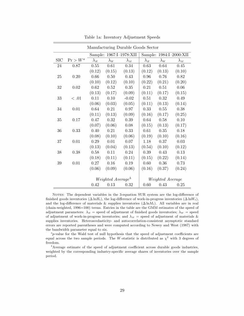
Table 1a: Inventory Adjustment Speeds

Manufacturing Durable Goods Sector

Sample: 1967:I–1978:XII Sample: 1984:I–2000:XIISIC Pr > W a λH λW λM λH λW λM24 0.87 0.55 0.61 0.34 0.63 0.64 0.45

(0.12) (0.15) (0.13) (0.12) (0.13) (0.10)25 0.20 0.66 0.50 0.43 0.96 0.76 0.82

(0.10) (0.12) (0.10) (0.22) (0.21) (0.20)32 0.02 0.62 0.52 0.35 0.21 0.51 0.06

(0.13) (0.17) (0.09) (0.11) (0.17) (0.15)33 < .01 0.11 0.10 -0.02 0.51 0.32 0.49

(0.06) (0.03) (0.05) (0.11) (0.13) (0.14)34 0.01 0.64 0.21 0.97 0.33 0.55 0.38

(0.11) (0.13) (0.09) (0.16) (0.17) (0.25)35 0.17 0.47 0.32 0.39 0.64 0.58 0.10

(0.07) (0.06) 0.08 (0.15) (0.13) (0.17)36 0.33 0.40 0.21 0.33 0.61 0.35 0.18

(0.08) (0.10) (0.06) (0.19) (0.10) (0.16)37 0.01 0.29 0.01 0.07 1.18 0.37 0.03

(0.13) (0.04) (0.13) (0.54) (0.10) (0.12)38 0.38 0.58 0.11 0.24 0.39 0.43 0.13

(0.18) (0.11) (0.11) (0.15) (0.22) (0.14)39 0.01 0.27 0.16 0.19 0.60 0.36 0.73

(0.06) (0.09) (0.06) (0.16) (0.37) (0.24)

Weighted Averageb Weighted Average0.42 0.13 0.32 0.60 0.43 0.25

Notes: The dependent variables in the 3-equation SUR system are the log-difference offinished goods inventories (∆ lnHt), the log-difference of work-in-progress inventories (∆ lnWt),and the log-difference of materials & supplies inventories (∆ lnMt). All variables are in real(chain-weighted, 1996=100) terms. Entries in the table are the GMM estimates of the speed ofadjustment parameters: λH = speed of adjustment of finished goods inventories; λW = speedof adjustment of work-in-progress inventories; and λM = speed of adjustment of materials &supplies inventories. Heteroscedasticity- and autocorrelation-consistent asymptotic standarderrors are reported parentheses and were computed according to Newey and West (1987) withthe bandwidth parameter equal to six.

ap-value for the Wald test of null hypothesis that the speed of adjustment coefficients areequal across the two sample periods. The W -statistic is distributed as χ2 with 3 degrees offreedom.

bAverage estimate of the speed of adjustment coefficient across durable goods industries,weighted by the corresponding industry-specific average shares of inventories over the sampleperiod.

29

Table 1b: Inventory Adjustment Speeds

Manufacturing Nondurable Goods Sector

Sample: 1967:I–1978:XII Sample: 1984:I–2000:XIISIC Pr > W a λH λW λM λH λW λM20 0.30 0.22 0.32 0.42 0.56 0.61 0.75

(0.20) (0.31) (0.12) (0.21) (0.18) (0.21)22 < .01 0.49 0.18 0.33 0.41 1.28 0.72

(0.09) (0.11) (0.10) (0.14) (0.21) (0.18)23 < .01 0.46 0.29 0.66 0.37 0.81 0.13

(0.12) (0.17) (0.13) (0.32) (0.19) (0.13)26 0.43 0.49 0.88 0.63 0.44 0.58 0.51

(0.08) (0.16) (0.11) (0.09) (0.14) (0.10)27 < .01 0.36 0.71 0.41 1.17 1.12 0.64

(0.12) (0.20) (0.10) (0.18) (0.20) (0.17)28 0.46 0.54 0.37 0.38 0.72 0.35 0.44

(0.03) (0.15) (0.12) (0.11) (0.15) (0.12)29 0.01 0.30 0.83 0.64 0.14 0.48 0.15

(0.15) (0.08) (0.13) (0.12) (0.16) (0.12)30 < .01 0.22 0.02 -0.07 0.31 0.60 0.38

(0.06) (0.10) (0.16) (0.12) (0.14) (0.13)31 0.06 0.45 0.28 0.48 0.54 0.83 0.49

(0.17) (0.15) (0.16) (0.17) (0.14) (0.11)

Weighted Averageb Weighted Average0.37 0.41 0.42 0.56 0.68 0.51

Notes: The dependent variables in the 3-equation SUR system are the log-difference offinished goods inventories (∆ lnHt), the log-difference of work-in-progress inventories (∆ lnWt),and the log-difference of materials & supplies inventories (∆ lnMt). All variables are in real(chain-weighted, 1996=100) terms. SIC 21 (Tobacco & Related Products) is omitted from theanalysis because of suspect data. Entries in the table are the GMM estimates of the speed ofadjustment parameters: λH = speed of adjustment of finished goods inventories; λW = speedof adjustment of work-in-progress inventories; and λM = speed of adjustment of materials &supplies inventories. Heteroscedasticity- and autocorrelation-consistent asymptotic standarderrors are reported parentheses and were computed according to Newey and West (1987) withthe bandwidth parameter equal to six.

ap-value for the Wald test of null hypothesis that the speed of adjustment coefficients areequal across the two sample periods. The W -statistic is distributed as χ2 with 3 degrees offreedom.

bAverage estimate of the speed of adjustment coefficient across durable goods industries,weighted by the corresponding industry-specific average shares of inventories over the sampleperiod.

30

Appendix

• Manufacturing Durable Goods Sector

1. SIC 24: Lumber and Wood Products

2. SIC 25: Furniture and Fixtures

3. SIC 32: Stone, Clay, and Glass Products

4. SIC 33: Primary Metal Industries

5. SIC 34: Fabricated Metal Products

6. SIC 35: Industrial Machinery and Equipment

7. SIC 36: Electronic and Other Electric Equipment

8. SIC 37: Transportation Equipment

9. SIC 38: Instruments and Related Products

10. SIC 39: Miscellaneous Durable Goods

• Manufacturing Nondurable Goods Sector

1. SIC 20: Food and Kindred Products

2. SIC 21: Tobacco and Related Products

3. SIC 22: Textile Mill Products

4. SIC 23: Apparel and Other Textile Products

5. SIC 26: Paper and Allied Products

6. SIC 27: Printing and Publishing

7. SIC 28: Chemicals and Allied Products

8. SIC 29: Petroleum and Coal Products

9. SIC 30: Rubber and Miscellaneous Plastic Products

10. SIC 31: Leather Products

31

1970 1972 1974 1976 1978 1980 1982 1984 1986 1988 1990 1992 1994 1996 1998 2000

0.5

1.0

1.5

2.0

2.5

3.0

3.5

Manufacturing Durable Goods Sector

Monthly Percent

Note: The vertical line at 1984:Q1 marks the estimated date of volatility reduction for durable goods GDP.

STD(output)*STD(sales)**STD(inv)***

1984:Q1

1970 1972 1974 1976 1978 1980 1982 1984 1986 1988 1990 1992 1994 1996 1998 2000

0.5

1.0

1.5

2.0

Manufacturing Nondurable Goods Sector

Monthly Percent

Note: The vertical line at 1986:Q3 marks the estimated date of volatility reduction for nondurable goods GDP.

STD(output)STD(sales)STD(inv)

1986:Q3

Figure 1

Volatility of Output, Sales, and Inventory Investment

* STD(output) denotes a rolling robust estimate of the standard deviation of the growth rate of output. ** STD(sales) denotes a rolling robust estimate of the standard deviation of the growth contribution of sales.*** STD(inv) denotes a rolling robust estimate of the standard deviation of the growth contribution of inventory investment.

1970 1972 1974 1976 1978 1980 1982 1984 1986 1988 1990 1992 1994 1996 1998 2000-0.4

-0.2

0.0

0.2

0.4

0.6

Manufacturing Durable Goods Sector

Monthly

Note: The vertical line at 1984:Q1 marks the estimated date of volatility reduction for durable goods GDP.

Corr(sales,inv)*

1984:Q1

1970 1972 1974 1976 1978 1980 1982 1984 1986 1988 1990 1992 1994 1996 1998 2000

-0.6

-0.4

-0.2

0.0

0.2

0.4

Manufacturing Nondurable Goods Sector

Monthly

Note: The vertical line at 1986:Q3 marks the estimated date of volatility reduction for nondurable goods GDP.

Corr(sales,inv)

1986:Q3

Figure 2

Inventory Investment and Sales Correlations

* Corr(sales,inv) denotes a rolling 5-percent trimmed correlation between the growth contribution of sales and the growth contribution of inventory investment.

1970 1972 1974 1976 1978 1980 1982 1984 1986 1988 1990 1992 1994 1996 1998 2000

0.3

0.4

0.5

0.6

0.7

0.8

0.9

Total Inventories

Monthly Percent

Note: The vertical line at 1984:Q1 marks the estimated date of volatility reduction for durable goods GDP.

STD(TOT-inv)*

1984:Q1

1970 1972 1974 1976 1978 1980 1982 1984 1986 1988 1990 1992 1994 1996 1998 20000.1

0.2

0.3

0.4

0.5

0.6

Growth Contributions of Inventories By Stage of Production

Monthly Percent

Note: The vertical line at 1984:Q1 marks the estimated date of volatility reduction for durable goods GDP.

STD(FG-inv)**STD(WP-inv)***STD(MS-inv)****

1984:Q1

Figure 3a

Inventory Volatility in Manufacturing Durable Goods Sector

* TOT-inv denotes the growth rate of total inventories. ** FG-inv denotes the growth contribution of finished goods inventories. *** WP-inv denotes the growth contribution of work-in-progress inventories.**** MS-inv denotes the growth contribution of materials and supplies inventories.STD() denotes a rolling robust estimate of the standard deviation.

1970 1972 1974 1976 1978 1980 1982 1984 1986 1988 1990 1992 1994 1996 1998 2000

0.3

0.4

0.5

0.6

0.7

0.8

Total Inventories

Monthly Percent

Note: The vertical line at 1986:Q3 marks the estimated date of volatility reduction for nondurable goods GDP.

STD(TOT-inv)*

1986:Q3

1970 1972 1974 1976 1978 1980 1982 1984 1986 1988 1990 1992 1994 1996 1998 2000

0.1

0.2

0.3

0.4

0.5

0.6

Growth Contributions of Inventories By Stage of Production

Monthly Percent

Note: The vertical line at 1986:Q3 marks the estimated date of volatility reduction for nondurable goods GDP.

STD(FG-inv)**STD(WP-inv)***STD(MS-inv)****

1986:Q3

Figure 3b

Inventory Volatility in Manufacturing Nondurable Goods Sector

* TOT-inv denotes the growth rate of total inventories. ** FG-inv denotes the growth contribution of finished goods inventories. *** WP-inv denotes the growth contribution of work-in-progress inventories.**** MS-inv denotes the growth contribution of materials and supplies inventories.STD() denotes a rolling robust estimate of the standard deviation.

1970 1972 1974 1976 1978 1980 1982 1984 1986 1988 1990 1992 1994 1996 1998 2000

25

30

35

40

45

50

Manufacturing Durable Goods Sector

Monthly Percent

FG-inv*WP-inv**MS-inv***

1970 1972 1974 1976 1978 1980 1982 1984 1986 1988 1990 1992 1994 1996 1998 2000

20

30

40

50

Manufacturing Nondurable Goods Sector

Monthly Percent

FG-inv WP-inv MS-inv

Figure 4

Inventory Composition by Stage of Production

* FG-inv denotes a rolling average (nominal) share of finished goods inventories. ** WP-inv denotes the a rolling average (nominal) share of work-in-progress inventories.*** MS-inv denotes a rolling average (nominal) share of materials and supplies inventories.

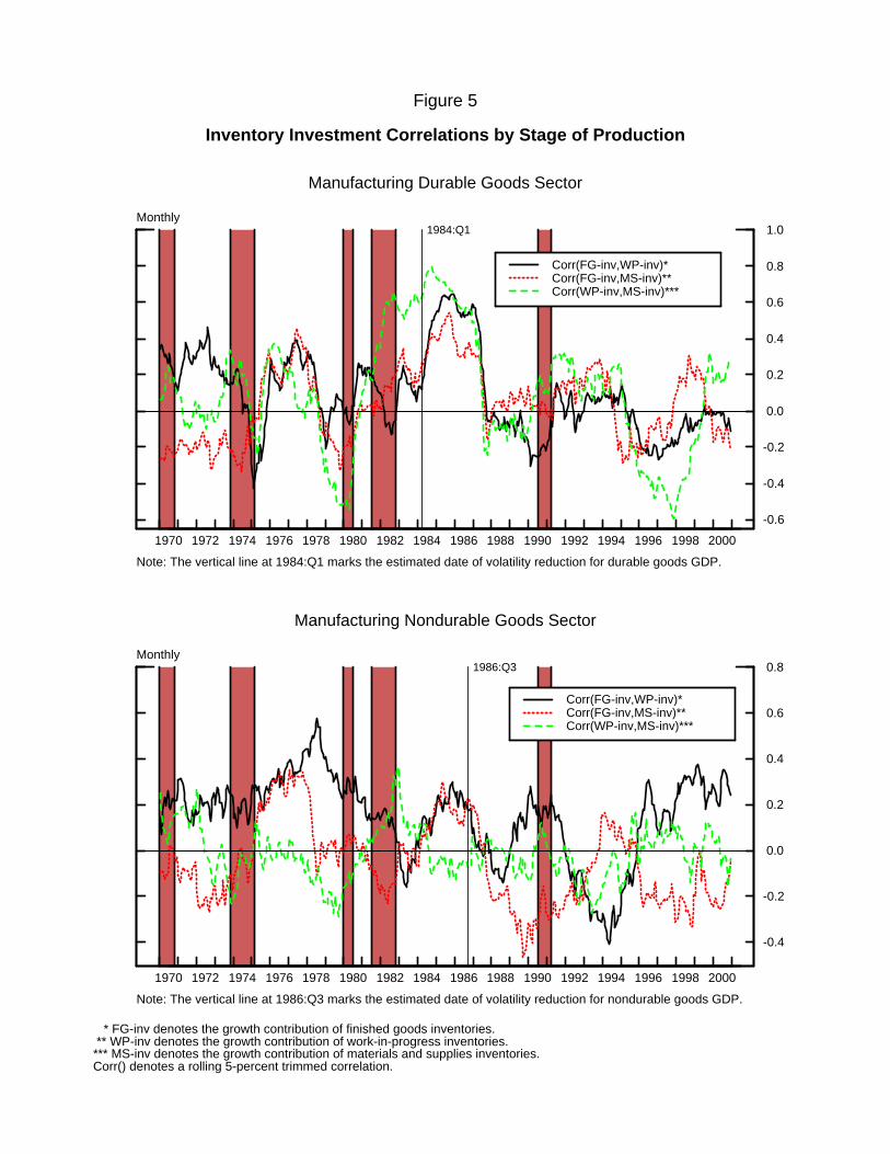
1970 1972 1974 1976 1978 1980 1982 1984 1986 1988 1990 1992 1994 1996 1998 2000

-0.6

-0.4

-0.2

0.0

0.2

0.4

0.6

0.8

1.0

Manufacturing Durable Goods Sector

Monthly

Note: The vertical line at 1984:Q1 marks the estimated date of volatility reduction for durable goods GDP.

Corr(FG-inv,WP-inv)*Corr(FG-inv,MS-inv)**Corr(WP-inv,MS-inv)***

1984:Q1

1970 1972 1974 1976 1978 1980 1982 1984 1986 1988 1990 1992 1994 1996 1998 2000

-0.4

-0.2

0.0

0.2

0.4

0.6

0.8

Manufacturing Nondurable Goods Sector

Monthly

Note: The vertical line at 1986:Q3 marks the estimated date of volatility reduction for nondurable goods GDP.

Corr(FG-inv,WP-inv)*Corr(FG-inv,MS-inv)**Corr(WP-inv,MS-inv)***

1986:Q3

Figure 5

Inventory Investment Correlations by Stage of Production

* FG-inv denotes the growth contribution of finished goods inventories. ** WP-inv denotes the growth contribution of work-in-progress inventories.*** MS-inv denotes the growth contribution of materials and supplies inventories.Corr() denotes a rolling 5-percent trimmed correlation.

0 6 12 18 24 30 36 42 48 54 60

-0.10

-0.05

0.00

0.05

0.10

Private Employment

Percent

Months After the Shock

Sample: 1967:I-1978:XIISample: 1984:I-2000:XII

0 6 12 18 24 30 36 42 48 54 60

-0.05

0.00

0.05

0.10

Price Level (PCE)

Percent

Months After the Shock

0 6 12 18 24 30 36 42 48 54 60

-0.5

0.0

0.5

1.0

1.5

Commodity Prices

Percent

Months After the Shock

0 6 12 18 24 30 36 42 48 54 60

-0.1

0.0

0.1

0.2

0.3

0.4

0.5

0.6

Federal Funds Rate

Percent

Months After the Shock

Figure 6a

Impulse Responses to a 50 bps. Federal Funds Rate ShockAggregate Block

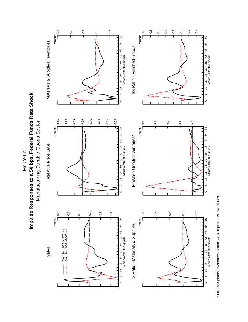
0 6

1218

2430

3642

4854

60

-0.4

-0.2

0.0

0.2

0.4

0.6

Sal

es

Per

cent

Mon

ths

Afte

r th

e S

hock

Sam

ple:

196

7:I-

1978

:XII

Sam

ple:

198

4:I-

2000

:XII

0 6

1218

2430

3642

4854

60

-0.2

0

-0.1

5

-0.1

0

-0.0

5

0.0

0

0.0

5

0.1

0

0.1

5

Rel

ativ

e P

rice

Leve

l

Per

cent

Mon

ths

Afte

r th

e S

hock

0 6

1218

2430

3642

4854

60

-0.2

0.0

0.2

0.4

0.6

Mat

eria

ls &

Sup

plie

s In

vent

orie

s

Per

cent

Mon

ths

Afte

r th

e S

hock

0 6

1218

2430

3642

4854

60

-0.5

0.0

0.5

1.0

1.5

I/S R

atio

- M

ater

ials

& S

uppl

ies

Per

cent

Mon

ths

Afte

r th

e S

hock

0 6

1218

2430

3642

4854

60

0.0

0.1

0.2

0.3

0.4

Fin

ishe

d G

oods

Inve

ntor

ies* P

erce

nt

Mon

ths

Afte

r th

e S

hock

0 6

1218

2430

3642

4854

60

-0.4

-0.2

0.0

0.2

0.4

0.6

0.8

1.0

I/S R

atio

- F

inis

hed

Goo

ds

Per

cent

Mon

ths

Afte

r th

e S

hock

Fig

ure

6bIm

pu

lse

Res

po

nse

s to

a 5

0 b

ps.

Fed

eral

Fu

nd

s R

ate

Sh

ock

Man

ufac

turin

g D

urab

le G

oods

Sec

tor

* F

inis

hed

good

s in

vent

orie

s in

clud

e w

ork-

in-p

rogr

ess

inve

ntor

ies.

0 6

1218

2430

3642

4854

60

-0.3

-0.2

-0.1

0.0

0.1

0.2

0.3

Sal

es

Per

cent

Mon

ths

Afte

r th

e S

hock

Sam

ple:

196

7:I-

1978

:XII

Sam

ple:

198

4:I-

2000

:XII

0 6

1218

2430

3642

4854

60

-0.1

0.0

0.1

0.2

0.3

0.4

Rel

ativ

e P

rice

Leve

l

Per

cent

Mon

ths

Afte

r th

e S

hock

0 6

1218

2430

3642

4854

60

-0.1

0.0

0.1

0.2

Mat

eria

ls &

Sup

plie

s In

vent

orie

s

Per

cent

Mon

ths

Afte

r th

e S

hock

0 6

1218

2430

3642

4854

60

-0.1

0.0

0.1

0.2

0.3

0.4

I/S R

atio

- M

ater

ials

& S

uppl

ies

Per

cent

Mon

ths

Afte

r th

e S

hock

0 6

1218

2430

3642

4854

60

-0.1

0.0

0.1

0.2

0.3

0.4

Fin

ishe

d G

oods

Inve

ntor

ies* P

erce

nt

Mon

ths

Afte

r th

e S

hock

0 6

1218

2430

3642

4854

60-0

.2

0.0

0.2

0.4

0.6

I/S R

atio

- F

inis

hed

Goo

ds

Per

cent

Mon

ths

Afte

r th

e S

hock

Fig

ure

6cIm

pu

lse

Res

po

nse

s to

a 5

0 b

ps.

Fed

eral

Fu

nd

s R

ate

Sh

ock

Man

ufac

turin

g N

ondu

rabl

e G

oods

Sec

tor

* F

inis

hed

good

s in

vent

orie

s in

clud

e w

ork-

in-p

rogr

ess

inve

ntor

ies.

Not

e: S

IC 2

1 (T

obac

co &

Rel

ated

Pro

duct

s is

om

itted

from

the

anal

ysis

bec

ause

of s

uspe

ct d

ata.

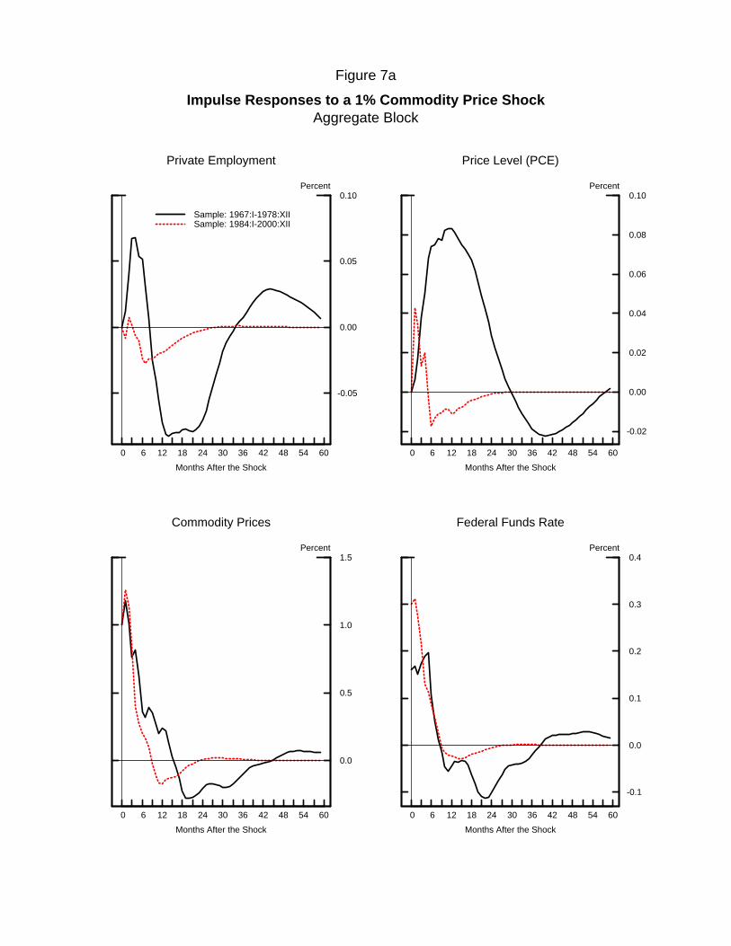
0 6 12 18 24 30 36 42 48 54 60

-0.05

0.00

0.05

0.10

Private Employment

Percent

Months After the Shock

Sample: 1967:I-1978:XIISample: 1984:I-2000:XII

0 6 12 18 24 30 36 42 48 54 60

-0.02

0.00

0.02

0.04

0.06

0.08

0.10

Price Level (PCE)

Percent

Months After the Shock

0 6 12 18 24 30 36 42 48 54 60

0.0

0.5

1.0

1.5

Commodity Prices

Percent

Months After the Shock

0 6 12 18 24 30 36 42 48 54 60

-0.1

0.0

0.1

0.2

0.3

0.4

Federal Funds Rate

Percent

Months After the Shock

Figure 7a

Impulse Responses to a 1% Commodity Price ShockAggregate Block

0 6

1218

2430

3642

4854

60-0

.3

-0.2

-0.1

0.0

0.1

0.2

0.3

0.4

Sal

es

Per

cent

Mon

ths

Afte

r th

e S

hock

Sam

ple:

196

7:I-

1978

:XII

Sam

ple:

198

4:I-

2000

:XII

0 6

1218

2430

3642

4854

60

-0.0

5

0.0

0

0.0

5

0.1

0

0.1

5

Rel

ativ

e P

rice

Leve

l

Per

cent

Mon

ths

Afte

r th

e S

hock

0 6

1218

2430

3642

4854

60-0

.2

-0.1

0.0

0.1

0.2

0.3

Mat

eria

ls &

Sup

plie

s In

vent

orie

s

Per

cent

Mon

ths

Afte

r th

e S

hock

0 6

1218

2430

3642

4854

60-0

.4

-0.2

0.0

0.2

0.4

0.6

I/S R

atio

- M

ater

ials

& S

uppl

ies

Per

cent

0 6

1218

2430

3642

4854

60-0

.10

-0.0

5

0.0

0

0.0

5

0.1

0

0.1

5

0.2

0

0.2

5

Fin

ishe

d G

oods

Inve

ntor

ies* P

erce

nt

Mon

ths

Afte

r th

e S

hock

0 6

1218

2430

3642

4854

60

-0.2

0.0

0.2

0.4

0.6

I/S R

atio

- F

inis

hed

Goo

ds

Per

cent

Mon

ths

Afte

r th

e S

hock

Fig

ure

7bIm

pu

lse

Res

po

nse

s to

a 1

% C

om

mo

dit

y P

rice

Sh

ock

Man

ufac

turin

g D

urab

le G

oods

Sec

tor

* F

inis

hed

good

s in

vent

orie

s in

clud

e w

ork-

in-p

rogr

ess

inve

ntor

ies.

0 6

1218

2430

3642

4854

60

-0.2

-0.1

0.0

0.1

0.2

0.3

Sal

es

Per

cent

Mon

ths

Afte

r th

e S

hock

Sam

ple:

196

7:I-

1978

:XII

Sam

ple:

198

4:I-

2000

:XII

0 6

1218

2430

3642

4854

60

0.0

0.1

0.2

0.3

Rel

ativ

e P

rice

Leve

l

Per

cent

Mon

ths

Afte

r th

e S

hock

0 6

1218

2430

3642

4854

60

-0.0

5

0.0

0

0.0

5

0.1

0

0.1

5

0.2

0

Mat

eria

ls &

Sup

plie

s In

vent

orie

s

Per

cent

Mon

ths

Afte

r th

e S

hock

0 6

1218

2430

3642

4854

60

-0.1

0.0

0.1

0.2

0.3

I/S R

atio

- M

ater

ials

& S

uppl

ies

Per

cent

Mon

ths

Afte

r th

e S

hock

0 6

1218

2430

3642

4854

60-0

.10

-0.0

5

0.0

0

0.0

5

0.1

0

0.1

5

Fin

ishe

d G

oods

Inve

ntor

ies* P

erce

nt

Mon

ths

Afte

r th

e S

hock

0 6

1218

2430

3642

4854

60

-0.2

-0.1

0.0

0.1

0.2

0.3

I/S R

atio

- F

inis

hed

Goo

ds

Per

cent

Mon

ths

Afte

r th

e S

hock

Fig

ure

7cIm

pu

lse

Res

po

nse

s to

a 1

% C

om

mo

dit

y P

rice

Sh

ock

Man

ufac

turin

g N

ondu

rabl

e G

oods

Sec

tor

* F

inis

hed

good

s in

vent

orie

s in

clud

e w

ork-

in-p

rogr

ess

inve

ntor

ies.

Not

e: S

IC 2

1 (T

obac

co &

Rel

ated

Pro

duct

s) is

om

itted

from

the

anal

ysis

bec

ause

of s

uspe

ct d

ata.