Inventory Control in a Multi-Supplier System - · PDF fileInventory Control in a Multi-Supplier System ... limitations and the use of different batch sizes between partners ... base

- 1 -

Inventory Control in a Multi-Supplier System

Yasemin Arda and Jean-Claude Hennet1

LAAS-CNRS, 7 Avenue du Colonel Roche, 31077 Toulouse Cedex 4, FRANCE

Abstract

An enterprise network is analyzed from the viewpoint of an end-product manufacturer who

receives customer orders and organises his production and supply policy so as to minimize the

sum of his average holding cost and average stock-out cost. For each main component to be

ordered, the producer has several possible suppliers. The arrivals of customers’ orders are

random and delivery times from suppliers are also supposed random. This supply system is

represented as a queuing network and the producer uses a base-stock inventory control policy

that keeps constant the position inventory level (current inventory level + pending

replenishment orders). The decision variables are the reference position inventory level and

the percentages of orders sent to the different suppliers. In the queuing network model, the

percentages of orders are implemented as Bernoulli branching parameters. A close-form

expression of the expected cost criterion is obtained as a complex non-linear function of

decision variables. A decomposed approach is proposed for solving the optimization problem

in an approximate manner. The quality of the approximate solution is evaluated by

comparison to the exact solution, which can be computed numerically in some simple cases,

in particular in the two-supplier case. Numerical applications show the important economic

advantage for the producer of sending orders to several suppliers rather than to a single one.

Keywords: Inventory Control, Supply Chain, Stochastic Models

1 Corresponding author : Jean-Claude Hennet, LAAS-CNRS, 7 Avenue du Colonel Roche, 31077 Toulouse Cedex 4, France, Tel :+33 561336313, Fax :+33 561636936, e-mail: [email protected].

13th Intl Working Seminar on Production Economics (WSPE), Igls, Autriche, pp.51-62

- 2 -

Inventory Control in a Multi-Supplier System

Yasemin Arda and Jean-Claude Hennet

LAAS-CNRS, 7 Avenue du Colonel Roche, 31077 Toulouse Cedex 4, FRANCE

Tel :+33 561336313, Fax :+33 561636936

e-mail: hennet (yarda)@laas.fr)

1. Introduction

A major difficulty in supply chain organisation and management is to conciliate global

efficiency with local autonomy. When considering a network of cooperating enterprises, a

basic objective is to organize integration in a non-compulsory manner, so as to maintain the

autonomy of partners. A possible approach for combining integration and autonomy is

through partly automated negotiation processes (Jennings et al, 2001, Besembel et al., 2002).

Once the negotiation has started, parameters can be updated and other criteria can enter into

play, such as costs (fixed and variable ordering costs), quality and non-formalized preference.

In such a way, the system complexity inherently attached to supply chain organization, can be

managed through negotiation between the main actors, each one of them basing his decision

upon a local optimization process. Such a scheme seems appealing by preserving the

autonomy and decision optimization among the partners of an Enterprise Network. However,

it has been shown to be globally sub-optimal (see e.g. Cachon and Zypkin, 1999), by driving

the system to a Nash equilibrium which can globally perform very poorly with respect to the

minimal total cost criterion. Several corrective actions have been proposed to compensate for

this bias. They mainly consist in sharing risks and costs among partners and this can be

implemented through contracts modifying local criteria in a globally more efficient manner

(Cachon and Lariviere, 2001, Chen et al., 2001).

Another well-known factor of inefficiency in supply chains is the so-called “bullwhip effect”,

which tends to propagate and amplify disturbances upward along the supply chain. A supply

chain generally involves several sources of disturbances, and coordination of product flows is

fragile since variations in external supply and demand may be amplified through

interconnections between partners. Some typical causes for such amplification are capacity

limitations and the use of different batch sizes between partners (Lee and Billington, 1992).


- 3 -

The study analyzes one of the basic elements of a supply chain: the operational relationships

between an end-producer and his direct suppliers. A simple queuing model is constructed,

based on the assumptions of a Poisson external demand for end-products, instantaneous

delivery to the customer from the producer’s stock and an exponentially distributed service

time for each supplier. Only one basic component of the end-product is considered and

suppliers are supposed equivalent in terms of quality and cost. They only differ by their

average service time. In spite of its simplicity, such a model grasps the main issues for the

producer: should he use only one supplier, the best one in terms of a relevant performance

index, or should he dispatch his orders between different suppliers? In the latter case, what

suppliers should be selected and for what percentage of the demand?

The potential usefulness of the model for the supplier is in the a-priori determination of his

“optimal” inventory level and of the volumes (or frequency) of his orders to suppliers, based

on a-priori evaluation of their average delivery time. In practice, this a-priori knowledge can

be considered as a starting point in the negotiation process that will be undertaken with the

suppliers. By assuming unitary demands and orders and memoryless arrival, dispatching and

service processes, we get rid of the bullwhip effect in the model, to concentrate on the mean

performance analysis. From the literature on the bullwhip effect, it is assumed that it can be

treated separately, through a more detailed model, either through synchronous scheduling

(Cachon, 1999) or/and through an adequate choice of batch sizes (Riddalls and Bennett,

2001).

To optimize the producer’s inventory level and the order dispatching proportions, it is

essential to combine the effects of random fluctuations on demand flows, and delays of

deliveries from suppliers. Random demands have often been considered in the existing

models of inventory control, specially the ones based on the “newsvendor” paradigm (Arrow

et al., 1951, Porteus, 1990). On the contrary, random delays in part deliveries have not often

been integrated in models explicitly. An exception is the work of Dolgui and Louly (2001), in

which several suppliers with random delivery delays are considered. In their work, the

different suppliers provide different parts to be assembled by the producers. Then, there is

interdependency between the inventory positions of the end product and of its components.

However, the inventory positions of the different components can be independently controlled

through the information and ordering system. On the contrary, the case of a centralized

inventory of a single component does not offer the same possibility of decomposition.

In this paper, a centralized inventory control model is constructed to combine supply and

demand randomness. The objective of the producer is to minimize his average cost by


- 4 -

constructing an ordering policy, defined by an optimal reference inventory position and a rule

for selecting the supplier of each inventory replenishment order.

Section 2 formulates the optimal inventory and ordering problem for one producer and several

suppliers. Then section 3 solves optimally the order dispatching problem in the particular

“make – to – order case, and an approximate resolution technique is presented in section 4 for

the make – to – stock case. The performance of the approximate solution is comparatively

evaluated on simple examples in section 5. Finally, some conclusions and perspectives are

presented.

2. The optimal inventory and ordering policy

The current inventory level of the product considered at time t is denoted I(t). It is defined as

the difference between the on-hand inventory and the amount of backorders. In general, an

ordering decision should not be based only on the inventory level. One should also consider

the number of replenishment orders which have been placed earlier and not yet been

delivered, denoted u(t). The global state of the system can then be characterized by the

inventory position, denoted P(t) defined by:

P(t) = I(t) + u(t) (1)

Depending on the information system available, an inventory position may be controlled at

any time through a continuous review policy, or at periodic times through a periodic review

policy. Then, the control policy determines when and how much to order. Different control

policies may be applied, within the limits of the legal agreements between producer and

supplier.

One of the most popular continuous review policy is the (s,S) policy, in which s stands for the

inventory position order point and S for the inventory position replenishment level. The base-

stock policy can be seen as a variant of the (s,S) policy, for which an order is placed whenever

a demand comes, so as to permanently maintain the inventory position S. This type of a policy

has been shown to be optimal under constant average demand rates or unitary demands with

independent identically distributed (i.i.d.) arrival dates, whenever the cost criterion only

depends on the inventory position (Axsater, 2000). Moreover, under unitary demands with

(i.i.d.) arrival dates, the optimal base stock policy reduces to the policy (s,S) with s = S-1.

This policy is denoted the reference inventory policy. It will be studied in the sequel, in the

multi-supplier case.


- 5 -

In the “make-to stock” context, when an order comes to the producer, it is immediately

satisfied if its amount is available in the stock. If not, it has to wait until the inventory has

been sufficiently replenished by the arrival of products from suppliers. In both cases, an order

is placed from the producer to the supplier whenever a demand comes and has the same

amount (1 in the unitary case). As shown in (Bollon et al., 2000), such a base stock control

policy can also be interpreted as a Kanban mechanism After an initial inventory

replenishment stage, the reference inventory policy maintains constant the inventory position

of the producer:

0 )( ttStP ≥∀= (2)

If the random processes of demand arrivals and supply deliveries are stationary, then, under a

stationary (S-1,S) base stock policy, the system (producer + suppliers) reaches stationary

conditions characterized by stationary probabilities of the number of orders placed by the

producer and not yet delivered by the suppliers. In the sequel, these probabilities will be

computed in the case of exponential distributions of demand arrivals and supply lead times.

From the producer viewpoint, the cost function to be minimized is the sum of the average

holding cost and the average stock-out cost. Consider the following notations:

I is the random variable representing the producer inventory level in stationary

conditions

u is the random variable representing the number of uncompleted orders from the

producer to the supplier in ergodic conditions

h is the unit holding cost,

b is the unit stock-out cost.

In stationary conditions under the (S-1,S) base stock policy, random variables I and w are

related by the following equality, derived from (1) and (2):

I=S-u (3)

Using notation (x)+ for max(x,0) and (x)- for max(-x,0), the average cost criterion takes the

form:

]b (I)E [ h (I)C(S) −+ += . (4)

Demands are assumed unitary. They enter the system as a Poisson process with rate λ > 0.

When a unitary demand arrives at time t, the producer serves it immediately if I(t)≥0. He

waits if I(t)<0. In both cases, he applies the (S-1,S) ordering policy by sending a

corresponding order to supplier i with probability αi satisfying 10 ≤≤ iα and ∑=

=N

1ii 1α . Such


- 6 -

unitary orders can be seen as a limit case that maximizes the information efficiency of order

transfer from the producer to the suppliers and minimizes the “bullwhip” effect by avoiding

transmission distortions due to differences in batch policies. Each supplier is supposed to have

an exponential service rate and treats the requests in the FIFO (First In First Out) order. Let μi

denote the mean service rate of supplier i = 1,…,N , with μi ≠ μj for j ∈ (1,…,i-1,i+1,…,N).

Such an order dispatching policy from the producer to the supplier is known as a Bernoulli

splitting process. A well known property of this process is {Ni(t), t ≥ 0} i = 1,…,N are Poisson

processes with rates piλ. Moreover, these processes are mutually independent.The proof of

this property can be found, in particular, in (Ross, 2000). As a consequence, each supplier can

be modelled as an M/M/1 queue with arrival rate αiλ and service rate μi. The set of suppliers

is represented as a network of N independent M/M/1 queues in parallel. The probability of

having ki orders in queue i is given by:

{ } μλα

μλα

i kkPi

ik

i

iii

i

⎟⎟⎠

⎞⎜⎜⎝

⎛−⎟⎟

⎠

⎞⎜⎜⎝

⎛== 1in orders Pr)( (5)

The necessary and sufficient condition for stability of queue i is αi ρi < 1, with ρi = λ / μi. The

probability for the network of queues to be in state { }Ni ,...,k,...,k,kkK 21= is given by the

product-form expression (Baskett et al, 1975):

)1()( ),...,( ii1

kii1 ραρα∏

=

−=N

iNkkP (6)

In the order dispatching problem, Bernoulli parameters α1, α2… αN are decision variables.

Their optimal values express the optimal assignment probabilities in steady state. The

considered optimization criterion is the sum of the mean holding cost and the mean stock-out

cost per time unit. The objective of the study is to compute the optimal Bernoulli parameters

and the optimal base stock value, S* minimizing the average cost criterion.

In the case of N suppliers, the number of orders not yet delivered to the producer is equal to

the total number of orders in the open queuing network composed by the queues of orders

coming from the producer. Let Ki denote the number of orders sitting in the ith supplier

queue. P(ki) = Pr{Ki = ki} is defined by equation (5). Then, the probability of having w orders

waiting in the suppliers queue is given by

{ } w...K Pr 21 =+++= Nw KKP

Probability Pw can be obtained by composition of the probabilities related to the N queues.

Such a composition can be computed from the probability generating function. Assuming


- 7 -

ji ραρα jjii ≠∀≠ , the product form (21) can be transformed into a sum as in (Kleinrock,

1975). Then one obtains (Arda and Hennet, 2003)

ρ )(N

1

1-wNi

1-wNN

1∑ ∏=

++

≠= ⎟⎟

⎟⎟

⎠

⎞

⎜⎜⎜⎜

⎝

⎛

×⎟⎟⎟

⎠

⎞

⎜⎜⎜

⎝

⎛

×=i

i

ijj

ijw bNHP α with ∏=

−=N

iii )ρα(H(N)

11 ,

jjkkkj ραρα

b−

=1 .(7)

The mean value of the number of pending orders is denoted Z, with

∑∞

=

==0

][w

wwPuEZ . (8)

Criterion (4) can be re-written:

S )b ( Z(S-w)Pb) (hC(S)S

ww −++= ∑

=0 (9)

and the following expression is obtained:

). ρ1ρ

( )ρ(1

)ρ-(1ρρ1ρS

)( ),...,,C(S,

N

1i ii

iiN

12

ii

Si

Si

Ni

Ni

ii

1-Ni

1-Ni

N

1

N21

Sbb

NHb)(h

iij

jij −

−+⎟⎟⎟⎟

⎠

⎞

⎜⎜⎜⎜

⎝

⎛

⎟⎟⎠

⎞⎜⎜⎝

⎛

−−

−×⎟⎟⎟

⎠

⎞

⎜⎜⎜

⎝

⎛

××+=

∑∑ ∏==

≠= α

αα

ααα

α

ααα

(10)

Convexity of criterion (10) with respect to variables α1,…, αN, S is not guaranteed in general.

Therefore, minimization of criterion (10) subject to constraints 10 ≤≤ iα for i=1,…, N and

∑=

=N

1ii 1α appears to be a hard optimization problem.

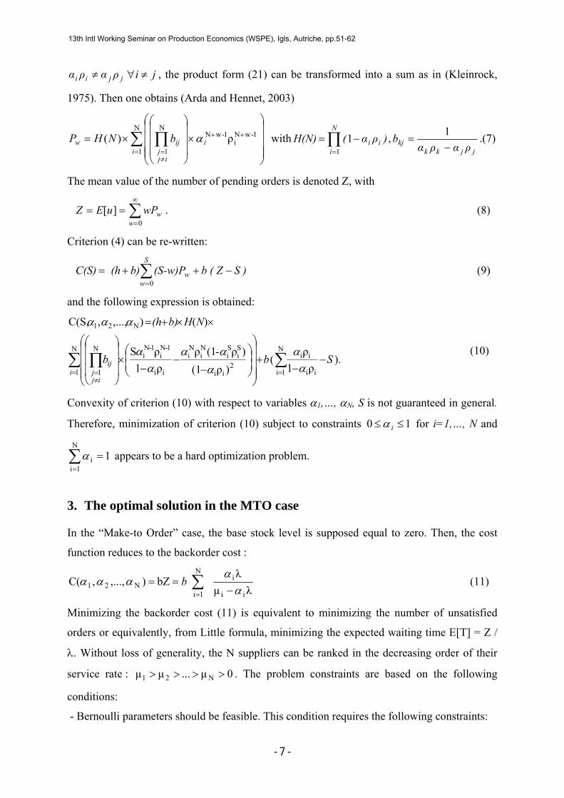
3. The optimal solution in the MTO case

In the “Make-to Order” case, the base stock level is supposed equal to zero. Then, the cost

function reduces to the backorder cost :

λμλ

bZ ),...,,C(ii

iN

1iN21 α

αααα

−== ∑

=

b (11)

Minimizing the backorder cost (11) is equivalent to minimizing the number of unsatisfied

orders or equivalently, from Little formula, minimizing the expected waiting time E[T] = Z /

λ. Without loss of generality, the N suppliers can be ranked in the decreasing order of their

service rate : 0μ...μμ N21 >>>> . The problem constraints are based on the following

conditions:

- Bernoulli parameters should be feasible. This condition requires the following constraints:


- 8 -

N1,...,i 10 i =≤≤α (12)

∑=

=N

1ii 1α (13)

- Stability of the queuing network requires the following conditions :

N1,...,i 1μλ

i=<iα

(14)

- Moreover, a necessary and sufficient condition for the existence of a set of Bernoulli

parameters, (αi ; i = 1,…,N) satisfying constraints (12), (13), and (14) is :

∑=

<N

1iiμλ (15)

Suppose that condition (15) is satisfied by the problem data. Then, the “Make-to Order”

optimization problem, denoted problem (P1) takes the following form :

λμ inimize

ii

iN

1i,...,1 αα

αα −∑=N

m (16)

under constraint (13), and constraint (17) which replaces (12) and (14) :

N1,...,i )λμ

1,min(0 i =≤≤ iα (17)

All the constraints are linear and in the feasible domain, criterion E[T] is convex:

3ii

i4

ii

iii2

ii

i2

2

λ)(μλ2μ

λ)(μ

λ)λ(μ2μλ)(μ

μ][ αα

αααα −

=−

−=⎟

⎟⎠

⎞⎜⎜⎝

⎛

−=

ii dd

dTEd .

Non negativity of 2

2 ][

idTEd

α is always guaranteed under constraint (14). Therefore, problem

(P1) is convex and has a unique minimum defined by the first order optimality conditions:

0][ =

idTEd

α for i=1,…,N under constraints (13), and (17).

3.1 Resolution of a relaxed problem

Consider now the case when the optimal solution of the problem defined by (16) and (13)

naturally satisfies condition (17). Then, this solution is optimal for problem (P1). The

Lagrangean of the relaxed problem can be written :


- 9 -

⎟⎟⎠

⎞⎜⎜⎝

⎛−−⎟⎟

⎠

⎞⎜⎜⎝

⎛−

= ∑∑==

N

1ii

ii

iN

1i1

λμ L α

αα

p

with p the Lagrange parameter associated with the equality constraint : ∑=

=N

1ii 1α . Let *

iα be

the optimal value of the Bernoulli parameter iα for i = 1,…,N. Then, the optimal solution of

the relaxed problem satisfies the following set of conditions:

N1,...,i 0λ)(μ

μL 2*

i

i ==−−

= pdd

ii αα (18)

∑=

=N

1i

* 1iα (19)

For any pair ( *iα , *

jα ), condition (18) can be re-written :

i

*ij*

j μ

λ)(μ μ λμ

ij

αα

−=− (20)

By summing over j both terms of equation (20), one obtains:

∑∑==

−=−

N

j

iN

jj

1 i

*ij

1

*j μ

λ)(μ μ λ)(μ

αα

Under constraint ∑=

=N

1i

* 1iα , this equation becomes : ∑∑==

−=−

N

j

iN

j 1j

i

*i

1j μ

μ λμ

λμα

and thus,

the following result is obtained.

Property 1 :

The optimal values of Bernoulli parameters with respect to the relaxed problem, are defined

by the following expressions:

N1,...,i )μ τ(μλ1

iNi* =−=iα (21)

where τN is defined by :

μ

λμ τ

N1j j

N1j j

N∑∑

=

=−

= (22)

If the optimal values (αi*) satisfy constraints (17), then the minimum of the relaxed problem

is feasible and therefore optimal for problem (P1). The feasibility condition is re-written:

N1,...,i )λμ

min(1,)μ τ(μλ10 i

iNi =≤−≤ (23)


- 10 -

From condition (13), τN > 0. Therefore, inequalities (23) can be replaced by :

N1,...,i λμ τμ0 iNi =≤−≤ (24)

meaning 10 * ≤≤ iα . The left-side inequality can be re written :

N1,...,i τμ 2Ni =≥ (25)

And, using ∑=

=N

1i

* 1iα , the right-side inequality becomes satisfied.

3.2 The restricted choice problem

From the ranking of service rates in the decreasing order 0μ...μμ N21 >>>> , if. inequality

(25) is not satisfied for i0, with Ni ≤≤ 01 , then, it is also violated for i = i0 +1,…,N. In this

case, the “restrictive choice problem” is obtained by imposing 0* =iα for i = i0,…,N To show

the relevance of the restricted choice problem, the following parameter is defined for

m=1,…,N+1, under the convention μN+1 = 0:

μ

λμ τ

m1j j

m1j j

m∑∑

=

=−

= (26)

The evolution of τm satisfies the following properties.

Property 2

For positive values of parameters τm et τm+1 (m ≤ N-1), the evolution of τm satisfies the

following rules :

(1) ⎪⎩

⎪⎨

⎧

<⇔

<⇔

<

++

+

+

21m1m

2m1m

m1m

τμ

τμ

τ τ

(2) ⎪⎩

⎪⎨

⎧

=⇔

=⇔

=

++

+

+

21m1m

2m1m

m1m

τμ

τμ

τ τ

(3) ⎪⎩

⎪⎨

⎧

>⇔

>⇔

>

++

+

+

21m1m

2m1m

m1m

τμ

τμ

τ τ

Proof

From (26), one obtains

λμμμ τμ τμ τ1m

1i1mi

m

1iim1mm

1m

1iim ∑∑∑

+

=+

=+

+

=

−−==− (27)

λμμμ τμ τμ τm

1i1mi

1m

1ii1m1m1m

m

1ii1m ∑∑∑

=+

+

=+++

=+ −+==+ (28)

this implies :


- 11 -

∑+

=+++ =−

1m

1iim1m1mm1m μ )τ-(τμ τμ (29)

∑=

++++ =−m

1iim1m1m1m1m μ )τ-(τ μ τμ (30)

The rules of property 2 directly derive from these two equalities.

Property 3 :

Parameter τm increases with m for 1 ≤ m ≤ m*. Then, parameter τm monotonously decreases

with m for m* < m ≤ N. The maximal value of parameter τm is obtained for m* (1 ≤ m* ≤ N),

which is the unique index satisfying:

*m2

*m1*m

*m

1ii μ τμ and λμ <≤> +

=∑ (31)

Proof :

The proof is presented in two parts.

i) Existence of the index m* :

For any set of parameters (λ, μ1,…, μN), condition (26) implies τN > 0. Let n be the smallest

index satisfying λμn

1ii∑

=

> . Replacing m + 1 by n in equation (31), one obtains:

∑=

=−1-n

1ii1-n μ )τ-(τ μ τμ nnnn (32)

From τn > 0 and τn-1 ≤ 0, equation (33) implies τμ 2n>n . If τμ 2

n1 ≤+n , then m* = n. If not,

relation τμ 2n1 >+n implies 2

1n1n τμ ++ > and n1n ττ >+ by the third rule of Property 2. And so,

the process is iterated for m = n + 2,…,N.

Then, starting from μN+1 = 0, we obtain τμ 2N1 ≤+N . Then, if 2

NN τμ > , m* = N. If not,

relation 2NN τμ ≤ implies 2

1-NN τμ ≤ et 1-Nττ ≤N from the first rule of Property 2. Thus, there

exists a unique index m*, with 1 ≤ m* ≤ N, that satisfies relations (31). Note that in the case

n = N, equation (32) implies τμ 21N+>N and thus m* = N.

ii) The evolution of parameter τm follows property 3.


- 12 -

For indices m=m*,…,N, relation λμμ *m1i i

m1i i ∑∑ ==

>> implies τm > 0.Then, from

2*m1*m τμ ≤+ , we can derive from Property 2, τm*+1 ≤ τm* and 2

1*m1*m τμ ++ ≤ Therefore, relation

21*m1*m2*m τμμ +++ ≤< implies τm*+2 < τm*+1. Applying the same reasoning for m =

m*+3,…,N, shows that parameter τm monotonously decreases with m for m* < m ≤ N.

According to equations (29) and (30), parameter τm increases with m for 1 ≤ m ≤ n-1, since μi

> 0 for i = 1,…,N. Then, knowing that τm > 0 for m = n,…,m* and that 2*m*m τμ > , one can

write τm* > τm*-1 and 2-1*m*m τμ > from Property 2. Consequently, relation 2

-1*m*m1*m τμμ >>−

implies τm*-1 > τm*-2. The same reasoning can then be applied to m = n,…,m*-3. And thus,

the value of parameter τm increases with m for 1 ≤ m ≤ m* and finally, the maximal value of

parameter τm is obtained for m*.

If condition (25) is not satisfied, the constrained problem can be solved using the following

property :

Property 4 :

Suppose that condition (13) is satisfied and consider the index m* (1 ≤ m* ≤ N) which satisfies

relations (31). Then, the optimal values of Bernoulli parameters are given by:

⎪⎩

⎪⎨⎧

+=

=−=

N1,...,*mifor 0

*m1,...,ifor )μ τ(μλ1 im*i*

iα (33)

Proof :

(i) Feasibility of policy *)(* mα defined by property 4 :

The set of Bernoulli parameters ( *iα ; i = 1,…,N) defined by (33) satisfies constraint (13) :

1)μ τμ(λ1)μ τ(μ

λ1 *

1ii*m

*m

1ii

*

1i*mi

1

* =−=−= ∑∑∑∑====

mm

i

N

iiα .

If m* = 1, the set ( 0,1 **1 == iαα for i = 2,…,N) is feasible. If m* > 1, since μi > μm* for i =

1,…m*-1 and 2*m*m τμ > , then 2

*m*mi τμμ >> which implies i*mi μ τμ > for i = 1,…m*.

From expression (33), it follows 0* >iα for i = 1,…m*. Moreover, the right side inequality of

constraint (15) is satisfied since τm* > 0. Thus, property 4 defines a feasible policy.

(ii) Optimality of policy *)(* mα :


- 13 -

From property 4, the policy *)(* mα is optimal if m* = N. For m* < N, from the convexity of

problem P1 with respect to parameters ,,...,1for , Njj =α , it suffices to show that the set of

values ( 0,...,0,,...,, **

*2

*1 mααα ) is locally optimal. So, consider an increase ∂αj > 0 with m* < j

≤ N. from policy *)(* mα . Then, constraint (13) implies a decrease of *iα for some i =

1,…,m* (∂αi < 0) under the following feasibility constraint:

0*

1=∂+∂ ∑

=

m

iij αα (34)

The criterion variation then takes the following form :

λ μλμ)λ(μ][

*

**

1*

*

jj

j

ii

im

i iii

iiTEα

α

αα

αααα

∂−

∂+⎟⎟⎠

⎞⎜⎜⎝

⎛

−−

∂+−

∂+=∂ ∑

=

(35)

or, equivalently,

λ μλ)μ)()λ(μ(μ

][ *

1**

jj

jm

i iiiii

iiTEα

α

αααα

∂−

∂+⎟⎟⎠

⎞⎜⎜⎝

⎛

−∂+−

∂=∂ ∑

=

(36)

From relations ∂αj > 0, ∂αi < 0, and expression (33), the following inequality is obtained.

j

jm

ii

j

jm

i

i

j

jm

i ii

iiTEμτ

1μτμλ)μ(

μ ][

*

12

*m

*

12

*m

*

12*

αα

ααα

αα ∂

+∂=∂

+⎟⎟⎠

⎞⎜⎜⎝

⎛ ∂=

∂+⎟⎟⎠

⎞⎜⎜⎝

⎛

−

∂>∂ ∑∑∑

===

(37)

Then, using equation (34), ∑=

α∂*m

1ii can be replaced by - jα∂ in inequality (37). And from

2*mj τμ ≤ for j = m*-1,…,N, we obtain :

0τ1

μ1][

2*m

>⎟⎟⎠

⎞⎜⎜⎝

⎛−∂>∂

jjTE α (38)

Therefore, the policy defined by parameters (33) is optimal.

4. An approximate solution in the “make-to-stock” case

The “make-to-stock” case corresponds to the general case, including the “make-to-order”

case, which can be characterized by a null base-stock level (S=0). Due to the complexity of

the cost function (10), it is proposed to decompose the problem into two parts. In the first part,

Bernoulli parameters are the decision variables while the base stock level is supposed to take

the zero value. These assumptions are the same as for Problem (P1). They correspond to the

MTO (Make to Order) case solved at the preceding section. In the second part of the problem;


- 14 -

denoted (P2), the values of Bernoulli parameters are supposed given and the only decision

variable to be determined is the base stock level. In this second part, the Bernoulli parameters

values obtained in (P1) are used as input data for problem (P2) and the optimal value of the

inventory capacity, S*, is computed using the discrete version of the “newsvendor” problem.

4.1 Computation of the dispatching parameters

Problem (P1) is solved as described in section 3. The value of m* is calculated by Property 3.

Then, the reference values of Bernoulli parameters are directly computed by explicit

expressions (33). The error derived from the application of this approximation scheme will be

evaluated in section 5.

4.2 Determination of the base stock level

From criterion expression (9), consider the incremental function )()1()( SCSCSG −+= . One

obtains: .Prob S) -b (ub) (hG(S) ≤+= The PDF F(S) = Prob{ u ≤ S } being a monotonous

increasing function, so is G(S). Then, the value S* for which C(S*) is optimal satisfies:

⎩⎨⎧

>⇔+<≤−⇔−≤

. 0)()1()(0)1()1()(

***

***

SGSCSCSGSCSC (39)

Therefore, a necessary and sufficient condition for optimality is given by the condition:

∑∑=

−

=

<+

≤**

0

1

0

S

ww

S

ww P

bhbP . (40)

For the order dispatching policy *)(* mα , expression (7) of wP leads to evaluation the

following quantity, from which the solution S* of Problem (P2) can be computed from (40):

ρ1

)ρ(1ρ )(m*

1 i

1Si

1i

1m*i

1m*i

m*

10∑ ∏∑=

++−−

≠== ⎟⎟

⎟⎟

⎠

⎞

⎜⎜⎜⎜

⎝

⎛

−−

×⎟⎟⎟

⎠

⎞

⎜⎜⎜

⎝

⎛

×=i i

S

ijj

ij

S

ww bNHP

ααα .

5. Evaluation of the Approximate Method

The approximation scheme described in section 4 relies on two simplifications. The first one

consists in replacing the global optimisation problem, with variables Nαα ,...,1 and S by an

independent problem (problem P1) in Nαα ,...,1 , followed by a problem in S (problem P2).

The second simplification consists in solving problem (P1) for a value of S (S=0) which is

not, in general, the optimal one. It can be noted that with the value of S imposed in problem


- 15 -

(P1), it is not possible to iterate the approximation scheme by updating the value of S. As a

consequence, the quality of the approximate solution is not guaranteed and there is a

possibility to identify some bias in the method. The approximate scheme has been evaluated

in the particular case of one producer and two suppliers. In this case, the global optimal

solution can be easily computed by exploration of the feasible domain (Arda and Hennet,

2003). Numerical evaluations reported on table 1, show an economic advantage for the

producer of sending orders to several suppliers rather than to a single one, even when the

second one is clearly less efficient than the first one. They also show that the approximation

method is satisfactory with an average deviation of less than 8% from the optimum, but a

strong tendency (more than 12%) to over-evaluate the dispatching parameters associated with

the most efficient suppliers.


- 16 -

α1 α2 S CriterionOptimal solution with 1 supplier 1,000 0,000 30,000 30,957Optimal solution with 2 suppliers 0,740 0,260 15,000 14,494

Sub-optimal solution with 2 suppliers 0,791 0,209 16,000 15,501Optimal solution with 1 supplier 1,000 0,000 30,000 30,957Optimal solution with 2 suppliers 0,698 0,302 14,000 13,275





Sub-optimal solution with 2 suppliers 0,667 0,333 8,000 8,049

Optimal solution with 1 supplier 1,000 0,000 9,000 9,955Optimal solution with 2 suppliers 0,845 0,155 9,000 8,614






Sub-optimal solution with 2 suppliers 0,828 0,172 8,000 7,953

Example 1 μ1=1.25 μ2=0.5

Example 2 μ1=1.25 μ2=0.6

Example 3 μ1=1.25 μ2=0.7

Example 4 μ1=1.25 μ2=0.8

Example 5 μ1=1.25 μ2=0.9

Example 6 μ1=1.25 μ2=1

Example 7 μ1=2 μ2=0.5





Example 12 μ1=2 μ2=1

Table 1 Comparative Results

6. Conclusions

Cooperation between the actors of a supply chain is a difficult problem due to the distributed

nature of the system and the associated degrees of decisional autonomy of the actors.


- 17 -

Negotiation can be seen as a basic tool to combine autonomy and integration. However, at the

present time, there is a lack of decision support tools for negotiation. In the particular case of

a negotiation between one producer and N suppliers, the producer needs to have a clear vision

of his own interest in terms of costs and delay. The study has shown that in the case of a

random demand from customers and random delivery delays from suppliers, it is generally

profitable to dispatch the orders between several suppliers rather than to direct all the

replenishment orders toward a single one. More specifically, the addressed problem was to

determine the percentages of orders to be directed toward each supplier and the base stock

level. An approximate technique has been proposed to solve this problem. Even if the quality

of this technique is satisfactory, an on-going research is devoted to its improvement.

References

Arda Y. and J.C. Hennet, (2003) Optimizing the ordering policy in a supply chain, LAAS

Report 03492.

Arrow, K., T. Harris and J. Marschak (1951). Optimal Inventory Policy. Econometrica, 19,

250-272.

Axsater, S. (2000). Inventory control. Ed. Kluwer Academic Publishers.

Baskett, F., K. M. Chandy, R. R. Muntz, F. G. Palacios (1975). Open, closed and mixed

networks of queues with different classes of customers. Journal of the Association for

Computing Machinery, 22, No. 2, 248 – 260.

Besembel, I., J.C. Hennet, E. Chacon (2002) Coordination by hierarchical negotiation within

an enterprise network, Proc. ICE 2002, Roma (Italia), 507-513.

Bollon J.M., M. Di Mascolo, Y. Frein, (2000) Unified formulation of pull control policies

using (min,plus) algebra, Proc. 15th IAR Annual Meeting, Nancy.

Cachon, G.P.(1999) Managing supply chain demand variability with scheduled order policies,

Management Science 45 (6) 843-856.

Cachon, G.P. and P.H. Zypkin, (1999) Competitive and cooperative inventory policies in a

two-stage supply chain, Management Science 45 (7) 936-953.

Cachon, G.P. and M. Lariviere, (2001), Contracts to assure supply: how to share demand

forecasts in a supply chain?, Management Science 47 (5) 629-646.

Chen, F., A. Federgruen and Y.S. Zheng, (2001), Coordination mechanisms for a distribution

system with ons supplier and multiple retailers, Management Science 47 (5) 693-708.


- 18 -

Dolgui A., M. A. Louly (2002), A model for supply planning under lead time uncertainty Int.

J. Production Economics 78 (2) 145-152.

Jennings, N.R., P. Faratin, A. R. Lomuscio, S. Parsons, C. Sierra and M. Wooldridge, (2001)

Automated negotiation: prospects, methods and challenges, Int. J. of Group Decision and

Negotiation 10 (2) 199-215.

Kleinrock, L. (1975). Queueing systems. Volume 1: Theory. Ed. John Wiley & Sons.

Lee, H.L., C. Billington, (1992) Managing the supply chain inventory: pitfalls and

opportunities, Sloan Management Review 33 (3) 65-73.

Porteus, E.L. (1990) Stochastic Inventory Theory, in Handbooks in operations research and

management science. Volume 2: Stochastic Models, Ed. North-Holland.

Riddalls, C.E., S. Bennett (2001) The optimal control of batched production and its effect on

demand amplification, Int. J. Production Economics 72, 159-168.

Ross, S.M. (2000) Introduction to probability models. Ed. A Harcourt Science and

Technology Company, Academic Press.


Documents

Inventory Control in a Multi-Supplier System - · PDF fileInventory Control in a Multi-Supplier System ... limitations and the use of different batch sizes between partners ... base