Embed Size (px)
Citation preview
DEFENSE LOGISTICS AGENCY Inventory Allocation and Forecasting
PREPARED BY
Brittney Cates
Derek Eichin
Matthew Mahoney
SPONSOR
Stephen Meyer, Defense Logistics Agency
FALL 2014
SYST/OR CAPSTONE PROJECT
1
TABLE OF CONTENTS
Executive Summary ...................................................................................................................................... 2
1. Introduction ........................................................................................................................................... 3
1.1 Sponsor ......................................................................................................................................... 3
1.2 Background ................................................................................................................................... 3
2. Problem Statement ................................................................................................................................ 4
3. Technical Approach .............................................................................................................................. 4
3.1 Literature Review .......................................................................................................................... 4
3.2 Data Exploration ........................................................................................................................... 4
3.2.1 Metrics .................................................................................................................................. 4
3.2.2 Data Reduction ...................................................................................................................... 7
3.2.3 Graphical Analysis ................................................................................................................ 9
3.3 Cluster Analysis .......................................................................................................................... 10
3.4 Model Development .................................................................................................................... 12
3.4.1 Model Inputs ....................................................................................................................... 12
3.4.2 Discrete Simulation Model ................................................................................................. 13
3.4.3 Optimization Using Stochastic Simulation Techniques ...................................................... 14
3.5 Testing and evaluation ................................................................................................................ 16
3.5.1 Model Runs ......................................................................................................................... 16
3.5.2 Results ................................................................................................................................. 17
3.5.3 Comparisons to SIMAN Model .......................................................................................... 20
4. Conclusions ......................................................................................................................................... 20
4.1 Recommendations ....................................................................................................................... 20
4.1.1 Recommended modifications to SIMAN Model ................................................................ 20
4.1.2 Recommended improvements to inventory policies ........................................................... 21
References ................................................................................................................................................... 22
Appendix A: Histograms of complete dataset ............................................................................................ 23
Appendix B: Cluster Analysis of complete dataset..................................................................................... 24
Appendix C: Further input analysis ............................................................................................................ 25
Appendix D: Graphical display of PMFs and analysis ............................................................................... 27
Appendix E: CDF SAS Script ..................................................................................................................... 30
Appendix F: Stochastic Optimization Model Matlab Script ....................................................................... 31

2
EXECUTIVE SUMMARY
Defense Logistics Agency’s (DLA) mission as a Joint Agency is complex and challenging. Their core
objective is to ensure that globally dispersed warfighters are able to conduct full spectrum operations in
any environment while maintaining a high quality of life. To better manage and apportion DLA’s
inventory across the globe, this study analyzed their current inventory allocation and forecast of major
end items. This objective lead the analysis down multiple lines of effort including cluster analysis to
logically and correctly group similar items; statistical analysis to understand the behavior of demand and
fulfillment of orders; heuristic analysis to derive key inventory measurements; and stochastic optimization
to identify the optimal solutions under constant uncertainty for these items.
In executing these tasks, new tools were developed for DLA to utilize in day-to-day inventory allocations
and forecasts. The tools enable DLA to derive probabilistic distributions from historical data sources and
incorporate them into inventory allocation simulations or heuristics; conduct what-if analysis on
probabilistic demand to determine budget or inventory requirements; and assess the outcomes from
decisions and the resulting Materiel Availability.
This study includes the development of a computationally scalable optimization using a stochastic
simulation; quick and intuitive output analysis with comparisons to historical cost and materiel
availability metrics; identification of major end items that do not require ordering over the course of a
year even under uncertain demand; and identification of major end items with so much variance in either
demand or fulfilment lead time that an optimal inventory ordering conditions could not be found.

3
1. INTRODUCTION
1.1 SPONSOR
The Defense Logistics Agency (DLA) is the Department of Defense’s (DoD) largest combat logistics
support agency. DLA jointly provides logistic support to the Army, Navy, Air Force, Marine Corps, other
federal agencies, as well as combined and allied forces with logistics, acquisition, and technical services.
DLA sources sustenance, fuel and energy, uniforms, medical supplies, and construction and barrier
equipment to our military, helping to maintain their ability to operate. DLA also supplies military spare
parts, manages restoration of military equipment, while additionally providing catalogs and production
services. DLA manages almost 5 million items, fills more than 131,000 requisitions per day, and issues
10,000 contract actions per day.
1.2 BACKGROUND
DLA is committed to supporting the warfighter, emphasizing the need for agency readiness by ensuring
supply chains are efficient and effective. DLA took their commitment further with a strategic
transformation in 2011, focusing on running a leaner, automated, and audit-ready business. The
implementation of this strategic plan enforces improvements by decreasing direct material costs,
decreasing operating costs, having the right size inventory, improving customer service, and achieving
audit readiness.
In identifying the right size inventory, DLA has determined that there is difficulty in maintaining Materiel
Availability (MA) of items with extreme demand. MA is the immediate availability and release of DLA
material against requisitions. Unfilled order levels, rate of filling customer orders, and inventory
inefficiency results in a significantly large amount of items remaining in backorder for multiple months,
with the root cause of the MA failures being unknown.
Many of the items with MA failures fall in the Acquisition Advice Code (AAC) D with Replenishment
Method Code (RMC) R National Item Identification Numbers (NIINs). The AAC category identifies the
stocking policy used for the item, with AAC D NIINs defined to be integrated materiel, which are
managed, stocked, and issued by the DoD. These items do not require specialized controls for shipment,
other than those imposed by the Integrated Materiel Manager (IMM)/service supply policy. DLA’s goal is
to have AAC D items available to the customer at all times. In the case that an AAC D item is
unavailable, a remedy plan should be in place to make that item available. The RMC category states
whether an item can be replenished or not. RMC R items can be replenished and forecasted.
4
2. PROBLEM STATEMENT
The purpose of this study was to assess DLA’s current methods and policies, identify necessary
improvements, and provide recommendations to increase the availability of items for customers. This
initiative was scoped to an analysis solely on AAC D and RMC R NIIN’s current inventory processes.
Since AAC D and RMC R NIINs have such high demand, improvements to these items’ current inventory
allocation and forecast will have the greatest effect on DLA’s inventory management.
3. TECHNICAL APPROACH
To assess DLA’s inventory management the study was separated into five efforts: literature review, data
exploration, cluster analysis, model development, and testing and evaluation.
3.1 LITERATURE REVIEW
The first objective of this study was to conduct a literature review to identify additional inventory metrics,
determine best practices for inventory management, understand the application of Coefficient of Variation
(CoV) when determining if a NIIN can be forecasted, and refine appropriate methods to use for cluster
analysis. The literature review identified On-hand Inventory Quantity, Inventory Turnover, and Days
Supply Inventory (DSI) as important inventory planning metrics [1]. In addition, setting the optimal
amount of safety stock in inventory is a driving factor in meeting demand.
The literature review also identified methods of cluster analysis. A Subject matter expert1 provided
recommendations in the most useful methods of cluster analysis with a strong preference to the K-means
algorithm. K-means is a heuristic algorithm that solves a predefined optimization function to determine if
data objects are more similar to others in the same cluster than to those in different clusters. Although, K-
means is sensitive to local minima, this method has proven to be an effective algorithm that does not
require extensive computation [2].
3.2 DATA EXPLORATION
3.2.1 METRICS
The analysis focused on understanding the impact from changes in contributing metrics on Materiel
Availability (MA). MA is calculated using equation 1. DLA’s goal is to maintain MA at 90% for aviation,
land, and maritime and 95% for industrial hardware.
1 Dr. Jie Xu, Assistant Professor, Systems Engineering and Operations Research Department, George Mason
University

5
Equation 1
𝑀𝐴 = [1 − (𝑢
𝑟)] ∗ 100%
Where,
𝑢= number of unfilled orders established (UFO)
𝑟= number of orders received
The contributing metrics that were of interest included: Production Lead Time (PLT), Total Lead Time
(TLT), Annual Demand Quantity (ADQ), Annual Demand Frequency (ADF), Back Orders Established
(BOE), Inventory on Hand (IOH), Lead Time Variance (LTV) (administrative and production), Demand
Value (DV), and Annual Demand Value (ADV).
a. Administrative Lead Time: ALT is the current average amount of time (in days) that it takes DLA
to process a Purchase Requisition (PR) for the National Stock Number (NSN) in question. ALT
starts on the date the PR is created and ends on the date the Purchase Order (PO) is created. It
consists of writing the Request for Proposal (RFP), receiving of bids, awarding of bids, and any
additional actions that make up the internal DLA process. The average for ALT is updated as POs
are filled.
b. Production Lead Time: PLT is the current average amount of time (in days) for the manufacturers
to produce and ship an item once the contract is awarded. PLT starts on the PO creation date to
the time when 51% or more of the PO quantity is received, also known as the date the Goods
Receipt (GR) is created. The average for PLT is updated at the GR creation date.
c. Total Lead Time: TLT is the entire time that it takes for an order to be placed and delivered. TLT
is calculated by summing ALT and PLT.
d. Annual Demand Quantity: ADQ is a metric that captures the amount of demand in a yearly
period. Demand is defined as an indication of a requirement, a requisition, or request for an item
of supply or individual item [3].
e. Annual Demand Frequency: ADF is a metric that captures the number of times demand was
requested for an item in a yearly period.
f. Back Orders Established: BOE are the number of back orders currently recorded for each NIIN.
A back order is established when the inventory does not have an item available when a requisition
is submitted; the item must be purchased and shipped for the requestor to receive the item.

6
g. Inventory on Hand: IOH identifies the current safety stock level in the inventory. This metric is
useful to identify the effects of varying safety stock levels have on back orders that get
established. Unfortunately this metric was unable to be captured from the data provided; therefore
IOH is excluded from the analysis. It is recommended that DLA investigate IOH in the future
since this metric has been identified as a useful metric for managing inventory.
h. Lead Time Variance: LTV is the variability in the lead times for either administrative (ALTV) or
production (PLTV) related tasks, or the combination of the two, for specific NIINs or Federal
Supply Codes (FSC). The FSC is identified in the national stock number, which is made up of the
concatenation of the FSC and NIIN values, and is another identifier for grouping similar systems
under this identifier. Lead time with high variance is indicative of data that has a large amount of
dispersion, which may be caused by spikes in the lead times. Higher probabilities for lengthy lead
time encourages DLA to manage higher safety stock levels for such items and ensure the items
will be available while requisitions are initiated. The variability for LTV is determined by
calculating the CoV for each NIIN. CoV is the ratio of the standard deviation to the mean; the
formula is shown in equation 2.
Equation 2
𝐶𝑜𝑉 =𝑠
�̅�
Where,
𝑠= sample standard deviation
�̅�= sample mean
i. Demand Value: DV is the value of the demand based on the individual prices and number of
requisitions made. DV is calculated using equation 3.
Equation 3
𝐷𝑉 = 𝑞 ∗ 𝑝 Where,
𝑞= requisition net quantity
𝑝= standard unit price
j. Annual Demand Value: ADV is defined as the value of the demand based on the price of the unit
and a sales unit conversion factor. ADV is calculated using equation 4.
7
Equation 4
𝐴𝐷𝑉 =𝑞
𝑓∗ 𝑝
Where,
𝑞= annual demand quantity
𝑓= sales unit conversion factor
𝑝= standard unit price
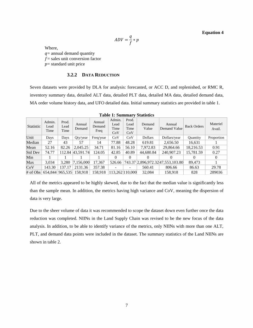
3.2.2 DATA REDUCTION
Seven datasets were provided by DLA for analysis: forecasted, or ACC D, and replenished, or RMC R,
inventory summary data, detailed ALT data, detailed PLT data, detailed MA data, detailed demand data,
MA order volume history data, and UFO detailed data. Initial summary statistics are provided in table 1.
Table 1: Summary Statistics
All of the metrics appeared to be highly skewed, due to the fact that the median value is significantly less
than the sample mean. In addition, the metrics having high variance and CoV, meaning the dispersion of
data is very large.
Due to the sheer volume of data it was recommended to scope the dataset down even further once the data
reduction was completed. NIINs in the Land Supply Chain was revised to be the new focus of the data
analysis. In addition, to be able to identify variance of the metrics, only NIINs with more than one ALT,
PLT, and demand data points were included in the dataset. The summary statistics of the Land NIINs are
shown in table 2.
Statistic Admin.
Lead
Time
Prod.
Lead
Time
Annual
Demand
Annual
Demand
Freq
Admin.
Lead
Time
CoV
Prod.
Lead
Time
CoV
Demand
Value
Annual
Demand Value Back Orders
Materiel
Avail.
Unit Days Days Qty/year Freq/year CoV CoV Dollars Dollars/year Quantity Proportion
Median 27 43 57 14 77.88 48.28 619.81 2,656.50 16,631 1
Mean 52.16 82.26 2,045.25 34.71 81.16 56.10 7,972.83 29,864.66 18,216.53 0.91
Std Dev 74.77 112.84 43,591.74 124.05 42.85 40.89 44,680.84 240,907.23 15,781.59 0.27
Min 1 1 1 1 0 0 0 0 0 0
Max 3,034 3,280 7,156,000 17,367 526.66 743.37 2,896,972.32 47,553,103.80 89,473 1
CoV 143.30 137.17 2131.36 357.38 - - 560.41 806.66 86.63 29.78
# of Obs 654,844 965,535 158,918 158,918 113,262 110,000 32,084 158,918 828 289036

8
Table 2: Land NIINs Summary Statistics
Stat Admin.
Lead
Time
Prod.
Lead
Time
Annual
Demand Annual
Demand Freq
Admin.
Lead
Time
CoV
Prod.
Lead
Time
CoV
Demand Value Annual
Demand
Value
Back
Orders Materiel
Avail.
Unit Days Days Qty/year Freq/year CoV CoV Dollars Dollars/year Quantity Proportion Median 6 11 85 22 1 2 $29,810 $8,578 0 1 Mean 23 44 2,170 81 2 4 $246,520 $73,628 1 .88 Std Dev 44 76 91,797 304 3 10 $1,634,199 $570,643 11 .28 Min 0 0 1 1 0 0 $0 $0 0 0 Max 1,806 2,300 7,156,000 16,104 110 519 $130,447,287 $47,533,104 454 1 CoV 1.93 1.72 42.3 3.75 - - 6.63 7.75 11 0.32
As shown in table 2, the current inventory policies for the Land NIINs are not being met at the 0.90 DLA
threshold level for MA since the mean value is 0.88. Improving the inventory policies for these NIINs are
necessary in order to ensure DLA is able to meet the Land Supply Chain threshold.
3.2.2.1 DATA REDUCTION ASSUMPTIONS
During data reduction, assumptions were made and captured to ensure consistency in the data reduction
procedures. The following lists the assumptions.
a. NIINs with ALT, PLT, ADQ, and ADF with a value of zero (0) were removed from the dataset.
Values of zero are not logical, as confirmed by the sponsor, since this would mean items would
not be forecasted or replenished. Such items may have a value of zero due to these items not
being purchased in a very long time, as confirmed by a DLA supply chain operator. DLA tracks
these NIINs despite not ordering these items for years or sometimes decades.
b. Observations in the ALT and PLT data with a negative value were removed from the dataset
when a sensible date could not be applied to resolve the value. Values that are negative are not
logical. A negative value for ALT would mean the administrative tasks were completed prior to
the RFP, which is not possible. It is assumed these records were inputted incorrectly into the
database, without further investigation it is unknown the true values for these data points.
c. Data points with empty NIIN or NSN were removed from the dataset. The dataset had many data
points that had empty fields for NIIN and NSN. Without further investigation the true values for
these NIINs are unknown.
d. Data points with null BOE values have a BOE of zero. The dataset had many null BOE fields, it
is assumed the value is zero when the field is blank or null.
e. Metrics with zeroes remaining in the dataset were deemed appropriate to that data point. For
example, value metrics have zeroes since there are standard unit values that cost zero, resulting in
zero values despite the demand being greater than zero. In addition, it is reasonable for variance
9
metrics to contain a value of zero. BOE has zero values when there are no back orders established
for the items when a requisition was initiated. And a value of zero for MA means the item was
unavailable when the customer requested it.
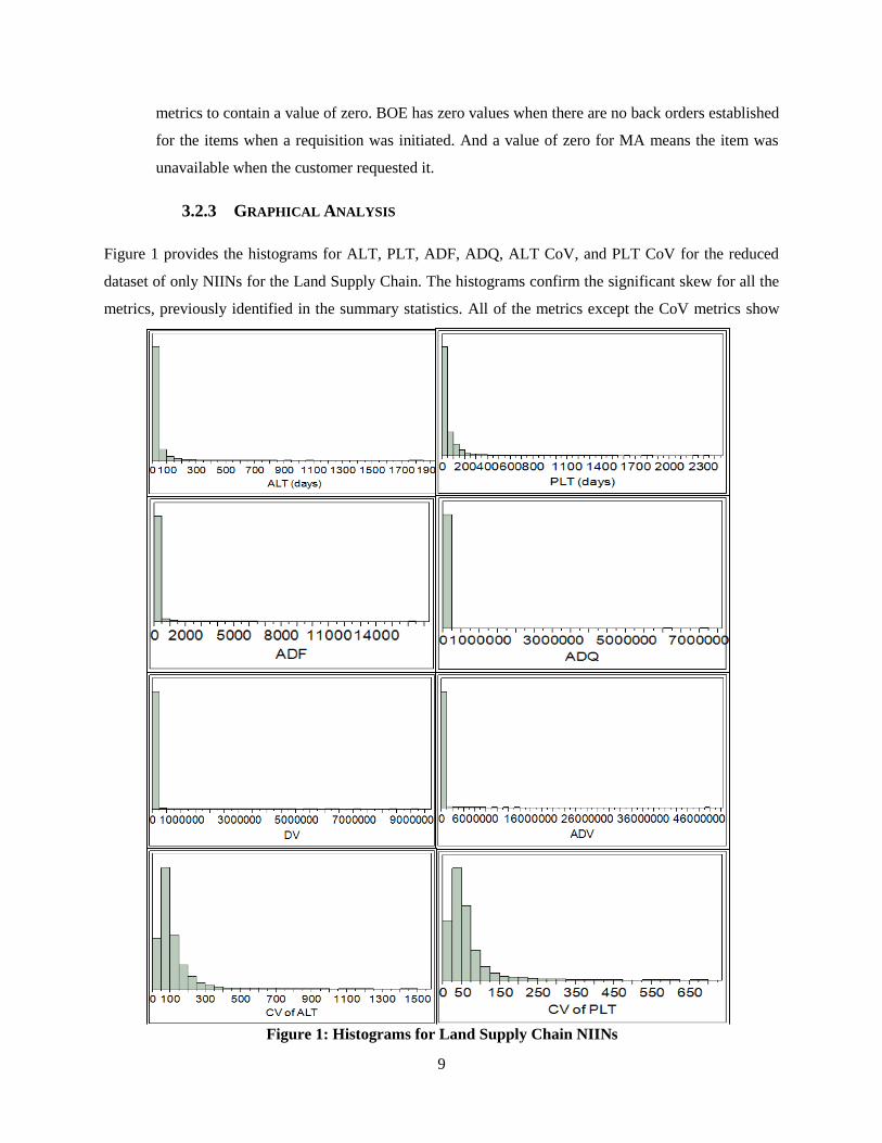
3.2.3 GRAPHICAL ANALYSIS
Figure 1 provides the histograms for ALT, PLT, ADF, ADQ, ALT CoV, and PLT CoV for the reduced
dataset of only NIINs for the Land Supply Chain. The histograms confirm the significant skew for all the
metrics, previously identified in the summary statistics. All of the metrics except the CoV metrics show
Figure 1: Histograms for Land Supply Chain NIINs

10
majority of the data being contained in the first few bars of the histogram. Additional input analysis is
provided in Appendix B, providing histograms of a the dataset with the outliers binned into one bin so
that the shape on a different scale can be visible. Histograms of the complete dataset of all NIINs are
provided in Appendix A.
3.3 CLUSTER ANALYSIS
DLA’s current division of AAC D NIINs are partitioned into categories by level of demand, which
includes super high, high, medium, and low demand. The team attempted to separate these items into
more groups to enable better forecasting and more accurate safety stock levels or policies through cluster
analysis.
The software JMP® by SAS® was used to identify AAC D clusters by the K-means method. K-means
was first used to identify clusters since this method was favorable to subject matter experts2, as
recognized during this study’s literature review process. JMP® calculates the Cubic Clustering Criterion
(CCC) a test statistic used to determine the number of clusters to use for each variable analyzed. The CCC
is the value that compares the observed coefficient of determination, also known as R2, to the approximate
expected R2 using a transformation method that stabilizes the variance [4].
JMP® takes into account the skew in the data by implementing the Johnson Transformation by bringing
data closer to the center of the dataset. In addition, JMP® takes into account data that is not in one unit by
identifying a common measurement scale by Columns Scaled Individually, if necessary [5]. Tables 3, 4,
and 5 provides the univariate cluster analysis for each variable of interest.
Table 3: CCC results
2 Dr. Jie Xu, Assistant Professor, Systems Engineering and Operations Research Department, George Mason
University
Number of clusters Admin
Lead
Time
Prod.
Lead
Time
Annual
demand
Quantity
Annual
Demand
Freq
Back
Orders ALT CoV PLT CoV
Demand
Value
Annual
Demand
Value
2 229.19 -70.43 -41.60* -47.12* -57.79 -39.65* -46.44* -163.96* -43.14*
3 300.21 -170.06 -47.80 -52.25 -47.26* -45.70 -51.49 -178.95 -49.97
4 349.19 -10.30 -51.66 -55.65 -65.99 -48.75 -53.56 -187.71 -54.81
5 360.04* 20.83 -55.29 -56.53 -49.91 -52.66 -56.59 -192.88 -56.59
6 316.57 87.45* -54.71 -53.97 -57.85 -54.35 -56.59 -196.44 -55.47
7 - 72.77 - - - - - - -
Note: Values marked with an asterisk (*) are the largest CCC, meaning this is the best cluster size. In addition,
negative values of this test statistic indicate a large number of outliers
11
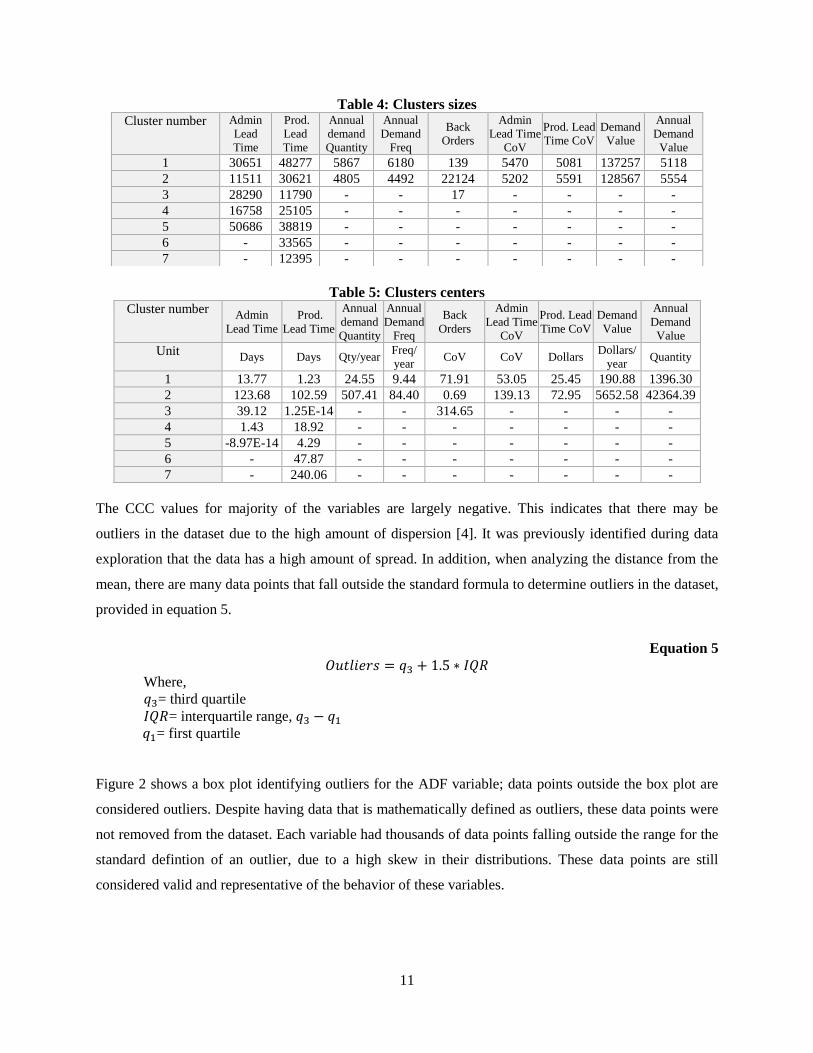
Table 4: Clusters sizes
Table 5: Clusters centers
The CCC values for majority of the variables are largely negative. This indicates that there may be
outliers in the dataset due to the high amount of dispersion [4]. It was previously identified during data
exploration that the data has a high amount of spread. In addition, when analyzing the distance from the
mean, there are many data points that fall outside the standard formula to determine outliers in the dataset,
provided in equation 5.
Equation 5
𝑂𝑢𝑡𝑙𝑖𝑒𝑟𝑠 = 𝑞3 + 1.5 ∗ 𝐼𝑄𝑅 Where,
𝑞3= third quartile
𝐼𝑄𝑅= interquartile range, 𝑞3 − 𝑞1
𝑞1= first quartile
Figure 2 shows a box plot identifying outliers for the ADF variable; data points outside the box plot are
considered outliers. Despite having data that is mathematically defined as outliers, these data points were
not removed from the dataset. Each variable had thousands of data points falling outside the range for the
standard defintion of an outlier, due to a high skew in their distributions. These data points are still
considered valid and representative of the behavior of these variables.
Cluster number Admin
Lead
Time
Prod.
Lead
Time
Annual
demand
Quantity
Annual
Demand
Freq
Back
Orders
Admin
Lead Time
CoV
Prod. Lead
Time CoV
Demand
Value
Annual
Demand
Value
1 30651 48277 5867 6180 139 5470 5081 137257 5118
2 11511 30621 4805 4492 22124 5202 5591 128567 5554
3 28290 11790 - - 17 - - - -
4 16758 25105 - - - - - - -
5 50686 38819 - - - - - - -
6 - 33565 - - - - - - -
7 - 12395 - - - - - - -
Cluster number Admin
Lead Time
Prod.
Lead Time
Annual
demand
Quantity
Annual
Demand
Freq
Back
Orders
Admin
Lead Time
CoV
Prod. Lead
Time CoV
Demand
Value
Annual
Demand
Value
Unit Days Days Qty/year
Freq/
year CoV CoV Dollars
Dollars/
year Quantity
1 13.77 1.23 24.55 9.44 71.91 53.05 25.45 190.88 1396.30
2 123.68 102.59 507.41 84.40 0.69 139.13 72.95 5652.58 42364.39
3 39.12 1.25E-14 - - 314.65 - - - -
4 1.43 18.92 - - - - - - -
5 -8.97E-14 4.29 - - - - - - -
6 - 47.87 - - - - - - -
7 - 240.06 - - - - - - -
12
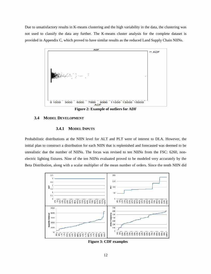
Due to unsatisfactory results in K-means clustering and the high variability in the data, the clustering was
not used to classify the data any further. The K-means cluster analysis for the complete dataset is
provided in Appendix C, which proved to have similar results as the reduced Land Supply Chain NIINs.
Figure 2: Example of outliers for ADF
3.4 MODEL DEVELOPMENT
3.4.1 MODEL INPUTS
Probabilistic distributions at the NIIN level for ALT and PLT were of interest to DLA. However, the
initial plan to construct a distribution for each NIIN that is replenished and forecasted was deemed to be
unrealistic due the number of NIINs. The focus was revised to ten NIINs from the FSC: 6260, non-
electric lighting fixtures. Nine of the ten NIINs evaluated proved to be modeled very accurately by the
Beta Distribution, along with a scalar multiplier of the mean number of orders. Since the tenth NIIN did
Figure 3: CDF examples

13
not follow any of the standard probability distributions, this NIIN was modeled separately using a discrete
cumulative distribution function (CDF).
CDFs for the remaining Land Supply Chain NIINs were modeled using SAS® software with the PROC
UNIVARIATE package. Figure 3 provides an example of CDFs for a component used on tanks.
Example PDFs, developed using Arena’s Input Analyzer, are shown below. Although these histograms
provide for adequate use of continuous distributions for these NIINs, the continuous distributions were
not used as part of the stochastic inputs to the models due the level of computation required to complete
all the NIINs in the dataset, and the loss of detail due to generalizing the historical data rather than using
it to define the behavior in the simulation.
Figure 4: PDFS for Order Quantity and Order Frequency respectively
All future discussion on stochastic inputs will be referencing the CDF method for the examples shown in
figure 3.
3.4.2 DISCRETE SIMULATION MODEL
The DLA Operations Research and Research Analysis (DORRA) developed the System of Integrated
Metrics Analysis (SIMAN) discrete simulation model to represent DLA’s current inventory management
processes and to analyze policy changes. The SIMAN model runs in both SAS® and Arena and models
the behavior at the NIIN level, rather than the each item level(per part) or supply chain level (multiple
NIINs). The SIMAN model provides results on MA and BOE based on ALT, PLT and other input values
fed into the model. It is not used to determine what MA should be; instead, it is the tool to determine

14
results on MA based on variations in ALT, PLT, or the other data elements. A disadvantage of this model
is that it does not currently incorporate stochastic demand processes with the application of probability
distributions. Instead, it utilizes the last two years of demand to assess the impact of new policies.
Since the SIMAN model only allowed discrete input variables, the model was modified to incorporate
stochastic variables. The CDFs previously identified, figure 3, were incorporated into the SIMAN model
in SAS® to account for variability in the data elements. This ensures that the SIMAN model will
incorporate the stochastic behavior of the inventory supply chain and provide accurate results of the
inventory metrics. This modification will also allow DORRA to be able to better analyze the effects on
the output variables in determining DLA’s inventory policies.
3.4.3 OPTIMIZATION USING STOCHASTIC SIMULATION TECHNIQUES
In addition to modifying the SIMAN model, a stochastic optimization of the simulation model was
developed to determine the optimal inventory policies for DLA. The model was built with three types of
ordering methods: consistent, triggered, and pre-emptive ordering. Figure 5 provides a notional example
of the ordering methods. Consistent ordering was used to model circumstances when a constant amount is
chosen to be ordered at a given interval. This type of ordering is the simplest for the customer to
implement and is considered the least powerful. When demand variance is small, meaning the data does
not have a large amount of dispersion, the constant amount is easier to identify and is intrinsically more
useful.
Triggered ordering was used to model circumstances that the inventory drops below a threshold, causing
an order to be generated which would return the inventory to a set holding level. This is harder for the
customer to implement than consistent ordering since it requires the customer to maintain awareness of
the current inventory levels; however, it is more powerful than consistent ordering. This type of ordering
allows for more variability in the demand. As the variability of the NIIN rises, an increased emphasis is
placed on the triggered ordering and away from the consistent ordering framework.
Pre-emptive ordering is used to model when an order is scheduled at a pre-appointed time to counteract a
historical surge in demand. This forces the customer to fully understand the behavior of the demand over
time; requiring more input by the customer up front. Pre-emptive ordering allows for more variability in
ALT and PLT, but is most effective when a time-dependent distribution is used. This will prove most
useful for excursion runs completed after the initial set of runs is completed.
15
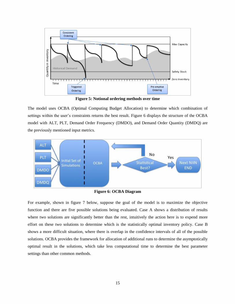
Figure 5: Notional ordering methods over time
The model uses OCBA (Optimal Computing Budget Allocation) to determine which combination of
settings within the user’s constraints returns the best result. Figure 6 displays the structure of the OCBA
model with ALT, PLT, Demand Order Frequency (DMDO), and Demand Order Quantity (DMDQ) are
the previously mentioned input metrics.
Figure 6: OCBA Diagram
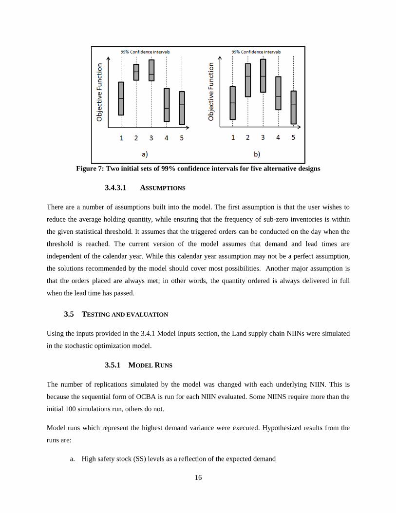
For example, shown in figure 7 below, suppose the goal of the model is to maximize the objective
function and there are five possible solutions being evaluated. Case A shows a distribution of results
where two solutions are significantly better than the rest, intuitively the action here is to expend more
effort on these two solutions to determine which is the statistically optimal inventory policy. Case B
shows a more difficult situation, where there is overlap in the confidence intervals of all of the possible
solutions. OCBA provides the framework for allocation of additional runs to determine the asymptotically
optimal result in the solutions, which take less computational time to determine the best parameter
settings than other common methods.
16
Figure 7: Two initial sets of 99% confidence intervals for five alternative designs
3.4.3.1 ASSUMPTIONS
There are a number of assumptions built into the model. The first assumption is that the user wishes to
reduce the average holding quantity, while ensuring that the frequency of sub-zero inventories is within
the given statistical threshold. It assumes that the triggered orders can be conducted on the day when the
threshold is reached. The current version of the model assumes that demand and lead times are
independent of the calendar year. While this calendar year assumption may not be a perfect assumption,
the solutions recommended by the model should cover most possibilities. Another major assumption is
that the orders placed are always met; in other words, the quantity ordered is always delivered in full
when the lead time has passed.
3.5 TESTING AND EVALUATION
Using the inputs provided in the 3.4.1 Model Inputs section, the Land supply chain NIINs were simulated
in the stochastic optimization model.
3.5.1 MODEL RUNS
The number of replications simulated by the model was changed with each underlying NIIN. This is
because the sequential form of OCBA is run for each NIIN evaluated. Some NIINS require more than the
initial 100 simulations run, others do not.
Model runs which represent the highest demand variance were executed. Hypothesized results from the
runs are:
a. High safety stock (SS) levels as a reflection of the expected demand

17
b. Frequent orders and relatively low Economic Order Quantity (EOQ) as a reflection of
expected lead times and demand
c. Low MA and high BOE due to frequent reorders
MA and the number of BOEs were identified from these model runs to understand the impact of high
demand on variance. The results of these model runs supported an analysis into the appropriate SS levels
and EOQ for NIINs that did not meet MA.
The second set of model runs was to represent moderate demand variance. Hypothesized results from the
runs are:
a. Low SS levels as a reflection of the expected demand
b. Nominal number of orders and relatively low EOQ as a reflection of lead times and demand
c. High MA and low BOEs due to predictable reorder point and forecasted demand
The same analysis was done for these model runs as for the high demand variance runs. Lastly, model
runs to represent little to no demand variance were run. Hypothesized results from the runs are:
a. Minimal SS levels due to the predictability of the demand
b. Near constant number of orders and an EOQ as a factor of the demand and lead time
c. Maximized MA and Minimized BOE due to the predictable demand
These runs have the highest MA and eliminate BOE and SS, while providing enough information to
identify optimal EOQ.
3.5.2 RESULTS
The objective of the optimization model was set to minimize the holding cost, which is defined here as
the average number of items held over the period of time. When the holding cost resulted in a value of
10,000,000 the MA is not being met. This means that even with reorders to the maxium capacity up to
four times the expected monthly average, the inventory is unable to be maintained at a 90% MA level.
The initial order quantity was set to be the maxium capacity of the inventory holding. The maxium
capacity (upper bound), safety stock (lower bound), and monthly reorder quantity for the constant
reorders were set, with the summary statistics for these inputs shown in the table below. The output of the
optimization model is the average number of orders placed over the course of one year.

18
Table 6: Order quantity summary statistics
The distribution of the results for the average number of orders is shown in figure 6.
Figure 6: Histogram of order quantity
Of the 10672 NIINs modeled, 2630 resulted in a MA less than 90%, meaning these NIINs were unable to
maintain sufficient inventory to meet the DLA defined threshold for MA. In other words, 75% of the
Land Supply Chain NIINs would meet MA within the model’s contraints.
K-means cluster analysis was implemented on the output of the optimization model, order quantity.
Although, clustering did not provide sufficient evidence of obvious categorizations in the input data, it
was recommended to investigate the output of the optimization model for any obvious groupings. The
results of the cluster analysis are provided in tables 7, 8, and 9 below.
Statistic Holding Upper Bound Lower Bound Constant Reorder Orders
Unit Average quantity Quantity Quantity Quantity Average quantity
Median 25.5 40.0 10.0 5.0 14.0
Mean 193.7 48.9 21.9 54.3 9.7
Std Dev 1139.9 37.7 28.7 276.3 7.1
Min 3.4 0.0 0.0 0.0 0.0
Max 29924.3 210.0 200.0 5500.0 41.0
CoV 5.9 0.8 1.3 5.1 0.7
# of Obs 8042 8042 8042 8042 8042
19
Table 7: CCC results
Table 8: Clusters sizes
Table 9: Clusters centers
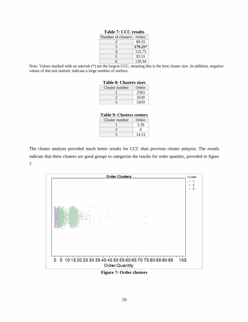
The cluster analysis provided much better results for CCC than previous cluster anlaysis. The resutls
indicate that three clusters are good groups to categorize the results for order quantity, provided in figure
7.
Figure 7: Order clusters
Number of clusters Orders
2 89.55
3 179.25*
4 125.75
5 93.31
6 126.94
Note: Values marked with an asterisk (*) are the largest CCC, meaning this is the best cluster size. In addition, negative
values of this test statistic indicate a large number of outliers
Cluster number Orders
1 2583
2 2630
3 5459
Cluster number Orders
1 3.39
2 0
3 14.53
20
Cluster 2 (the actual first cluser on the graph in red) are NIINs that resulted in failed MA. The orders for
these NIINs are zero at the completion of the simulation since these NIINs were unable to maintain the
necessary inventory to reach the avialability of 90%. The next cluster are NIINs that were able to
maintain MA with just an average number of orders ranging from one to three. Then all NIINs with three
or more orderes were grouped into the last cluster
As a result of the stochastic optimization model on Land Supply Chain NIINs would be recommended for
DLA to pay closer attention to NIINs in cluster 2 and 3. Cluster 2 represents the the NIINs that are not
optimized by the OCBA model. Cluster 3 represents the NIINs require larger orders over the course of a
year in order to maintain MA.
3.5.3 COMPARISONS TO SIMAN MODEL
It is recommended that future studies focus on comparing the SIMAN model and the OCBA model. The
workload and turn time for data in addition to the total run time of the SIMAN model was greater than the
fixed amount of time the team had to conduct analysis and comparison.
4. CONCLUSIONS
When comparing the results from the OBCA model and the original values for annual demand value the
results from optimizing the reorder points while meeting demand shows a significant decrease in holding
cost and a nominal decrease in ordering cost. The Total holding cost was approximately $242,000,000
which is 25% of the total annual demand value, holding costs were not available for comparison and it is
recommended that they be tracked and made available for future studies. Similarly, the total ordering cost
was approximately $1,004,000,000 which is 5% less than the annual demand value. This indicates that
when considering ALT and PLT while executing procurements to uncertain demand the total ordering
cost should decrease.
4.1 RECOMMENDATIONS
4.1.1 RECOMMENDED MODIFICATIONS TO SIMAN MODEL
The following lists the recommendations for improving the SIMAN model:
a. Overall run time and conversion into a JAVA based simulation tool. The rationale for this
recommendation is due to the fact that SAS, while a very robust statistical analysis tool, is
extremely cumbersome on computation resources.
21
b. Converting certain SAS steps into the Structured Query Language (SQL) variant. The rationale
for this recommendation is due to the computational time necessary to complete certain steps like
appends and table merge.
c. Introducing an optimization model as the central focus for the generation of metrics. The
rationale for this recommendation is due to the SIMAN model being merely a reporting tool.
While this capability can be retained, decisions that result in improved reporting are more
valuable to decision makers, analysts, and inventory management professionals.
d. Adding a feature that allows for J33-Planning inventory or demand forecasts to be fed into the
model rather than depending on deterministic demand values from a set time period that may not
be a correct comparison. The rationale for this recommendation is to enable a collaborative
“What-If” analysis process for the Planning and Order Sustainment branches of the DLA J-33
directorate. The establishment of such a process will ensure both the plans and operations are
synchronized and each branch understands the ramifications of their individual decisions or
business processes.
4.1.2 RECOMMENDED IMPROVEMENTS TO INVENTORY POLICIES
As a result of the stochastic optimization model analysis, the following recommendations were identified:
a. Improve execution of inventory planning by conducting more frequent discussions with the J-33
Plans directorate and constructing a framework that allows J-33 Operations and Plans to access
each others data.
b. Integration of IOH into planning and modeling. This will enable better monitoring of stock and in
the future establish reorder points for high demand NIINs.

22
REFERENCES
[1] D. Shepard, “Collaborative Demand and Supply Planning Between Partners: Best Practices for
Effective Planning,” Michigan State University, Feb 2012.
[2] R. Xu, J. Xu, and D. Wunsch, “A Comparison Study of Validity on Swarm Intelligence-Based
Clustering,” IEEE Trans. Systems, Man, and Cybernetics, vol. 2, no. 4, pp. 1243-1256, Aug 2012.
[3] “DoD Supply Chain Materiel Management Procedures: Operational Requirements,” Defense
Logistics Agency, DoD Manual, 4140.01, vol. 1, Feb 2014.
[4] “SAS® Technical Report A-108 Cubic Clustering Criterion,” Cary, NC; SAS Institute Inc., 1983, pp
56.
[5] “K-means Clustering,” Cary, NC; JMP® Statistical Discovery from SAS, 2014,
http://www.jmp.com/support/help/K-Means_Clustering.shtml

23
APPENDIX A: HISTOGRAMS OF COMPLETE DATASET
As stated earlier, the dataset was reduced due to the sheer volume of data to only Land Supply Chain
NIINs. Prior to the reduction of the dataset the complete dataset with all NIINs was plotted to understand
the shape and spread of the data. The figure below provides the histograms of the input metrics.
Figure 8: Histograms for the complete dataset
24
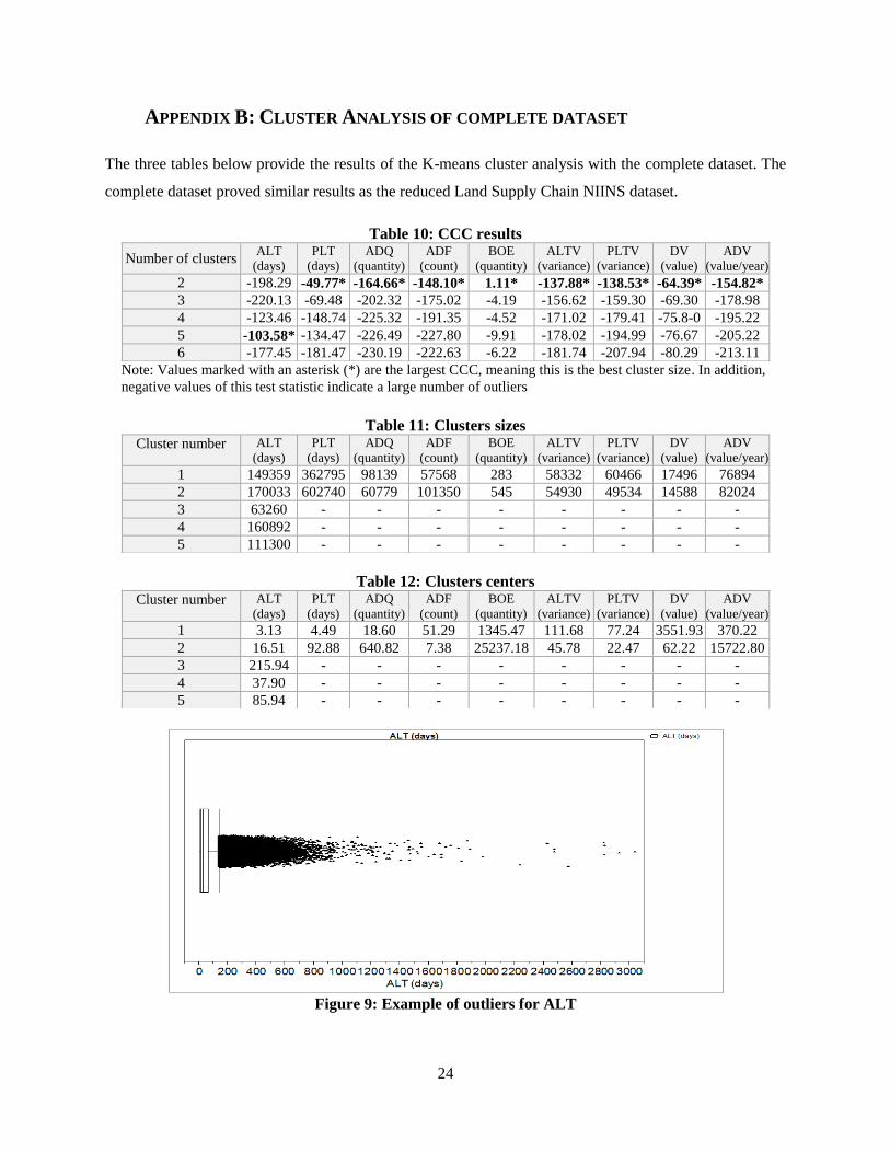
APPENDIX B: CLUSTER ANALYSIS OF COMPLETE DATASET
The three tables below provide the results of the K-means cluster analysis with the complete dataset. The
complete dataset proved similar results as the reduced Land Supply Chain NIINS dataset.
Table 10: CCC results
Table 11: Clusters sizes
Table 12: Clusters centers
Figure 9: Example of outliers for ALT
Number of clusters ALT
(days)
PLT
(days)
ADQ
(quantity)
ADF
(count)
BOE
(quantity)
ALTV
(variance)
PLTV
(variance)
DV
(value)
ADV
(value/year)
2 -198.29 -49.77* -164.66* -148.10* 1.11* -137.88* -138.53* -64.39* -154.82*
3 -220.13 -69.48 -202.32 -175.02 -4.19 -156.62 -159.30 -69.30 -178.98
4 -123.46 -148.74 -225.32 -191.35 -4.52 -171.02 -179.41 -75.8-0 -195.22
5 -103.58* -134.47 -226.49 -227.80 -9.91 -178.02 -194.99 -76.67 -205.22
6 -177.45 -181.47 -230.19 -222.63 -6.22 -181.74 -207.94 -80.29 -213.11
Note: Values marked with an asterisk (*) are the largest CCC, meaning this is the best cluster size. In addition,
negative values of this test statistic indicate a large number of outliers
Cluster number ALT
(days)
PLT
(days)
ADQ
(quantity)
ADF
(count)
BOE
(quantity)
ALTV
(variance)
PLTV
(variance)
DV
(value)
ADV
(value/year)
1 149359 362795 98139 57568 283 58332 60466 17496 76894
2 170033 602740 60779 101350 545 54930 49534 14588 82024
3 63260 - - - - - - - -
4 160892 - - - - - - - -
5 111300 - - - - - - - -
Cluster number ALT
(days)
PLT
(days)
ADQ
(quantity)
ADF
(count)
BOE
(quantity)
ALTV
(variance)
PLTV
(variance)
DV
(value)
ADV
(value/year)
1 3.13 4.49 18.60 51.29 1345.47 111.68 77.24 3551.93 370.22
2 16.51 92.88 640.82 7.38 25237.18 45.78 22.47 62.22 15722.80
3 215.94 - - - - - - - -
4 37.90 - - - - - - - -
5 85.94 - - - - - - - -

25
APPENDIX C: FURTHER INPUT ANALYSIS
The histograms of the data did not provide very much information due to the data being contained in only
a few bars because of the extreme spread of the data. Because of this, the histograms were zoomed in to
the majority of the data to understand the behavior. These histograms visually remove the outliers by
binning them into the ‘more’ bin. The histograms provided in Figure 10 show there is some shape to the
data. The figure below are the condensed historgrams for ALT, PLT, ADF, ADQ, BOE, ALT CoV, and
PLT CoV.
Figure 10. Condensed histograms of input data
-
10,000
20,000
30,000
40,000
50,000
60,000
Num
ber o
f O
bser
vati
ons
Days
ALT
-
10,000
20,000
30,000
40,000
50,000
Num
ber o
f O
bser
vati
ons
Days
PLT
- 1,000 2,000 3,000 4,000 5,000 6,000 7,000
Num
ber o
f O
bser
vati
ons
Frequency
ADF
- 1,000 2,000 3,000 4,000 5,000 6,000
Num
ber o
f O
bser
vati
ons
Quantity
ADQ
-
5,000
10,000
15,000
20,000
0 1 5 10 25 50 100 200 300 400 More
Num
ber o
f O
bser
vati
ons
Number of Orders
BOE
-
2,000
4,000
6,000
8,000
1 2 3 4 5 6 7 8 9 10 More
Num
ber o
f O
bser
vati
ons
CoV
ALTV
-
2,000
4,000
6,000
8,000
10,000
12,000
1 2 3 4 5 6 7 8 9 10 MoreNum
ber o
f O
bser
vati
ons
CoV
PLTV

26
The PLT and ALT distributions indicate that they have shape and look like they could be modeled by
either Gamma or Beta distribtuions if outliers were removed from the dataset. ADQ and ADF are
significantly skewed to the left indicating that there are major outliers within the set of Land NIINs from a
demand frequency and quantity perspective. The BOE histogram indicates that the vast majority of the
Land NIINs do not have matierel availability issues.
27
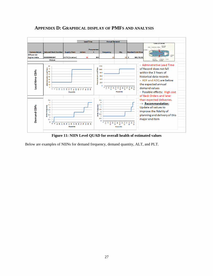
APPENDIX D: GRAPHICAL DISPLAY OF PMFS AND ANALYSIS
Figure 11: NIIN Level QUAD for overall health of estimated values
Below are examples of NIINs for demand frequency, demand quantity, ALT, and PLT.

28
Figure 12: PMFs of NIINs with high variance in Order Frequency
Figure 13: PMFs of NIINs with high variance in Order Quantity
29
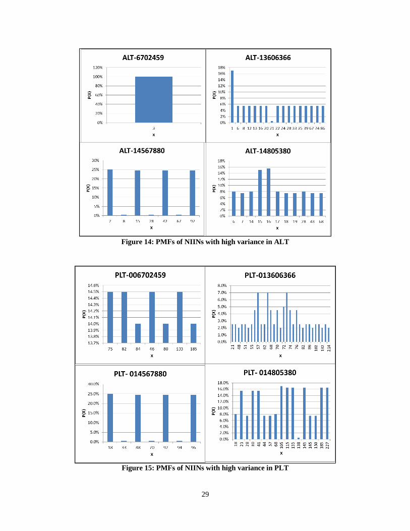
Figure 14: PMFs of NIINs with high variance in ALT
Figure 15: PMFs of NIINs with high variance in PLT
30
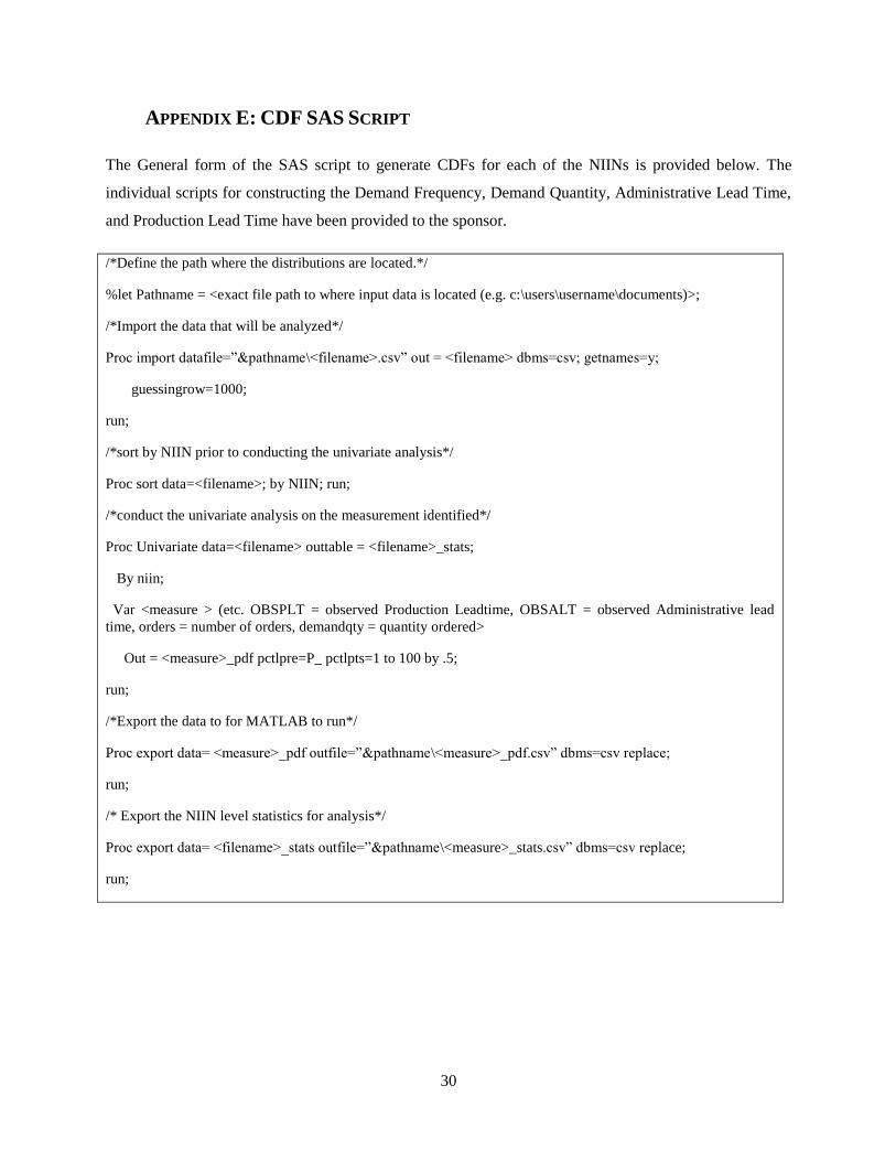
APPENDIX E: CDF SAS SCRIPT
The General form of the SAS script to generate CDFs for each of the NIINs is provided below. The
individual scripts for constructing the Demand Frequency, Demand Quantity, Administrative Lead Time,
and Production Lead Time have been provided to the sponsor.
/*Define the path where the distributions are located.*/
%let Pathname = <exact file path to where input data is located (e.g. c:\users\username\documents)>;
/*Import the data that will be analyzed*/
Proc import datafile=”&pathname\<filename>.csv” out = <filename> dbms=csv; getnames=y;
guessingrow=1000;
run;
/*sort by NIIN prior to conducting the univariate analysis*/
Proc sort data=<filename>; by NIIN; run;
/*conduct the univariate analysis on the measurement identified*/
Proc Univariate data=<filename> outtable = <filename>_stats;
By niin;
Var <measure > (etc. OBSPLT = observed Production Leadtime, OBSALT = observed Administrative lead
time, orders = number of orders, demandqty = quantity ordered>
Out = <measure>_pdf pctlpre=P_ pctlpts=1 to 100 by .5;
run;
/*Export the data to for MATLAB to run*/
Proc export data= <measure>_pdf outfile=”&pathname\<measure>_pdf.csv” dbms=csv replace;
run;
/* Export the NIIN level statistics for analysis*/
Proc export data= <filename>_stats outfile=”&pathname\<measure>_stats.csv” dbms=csv replace;
run;
31
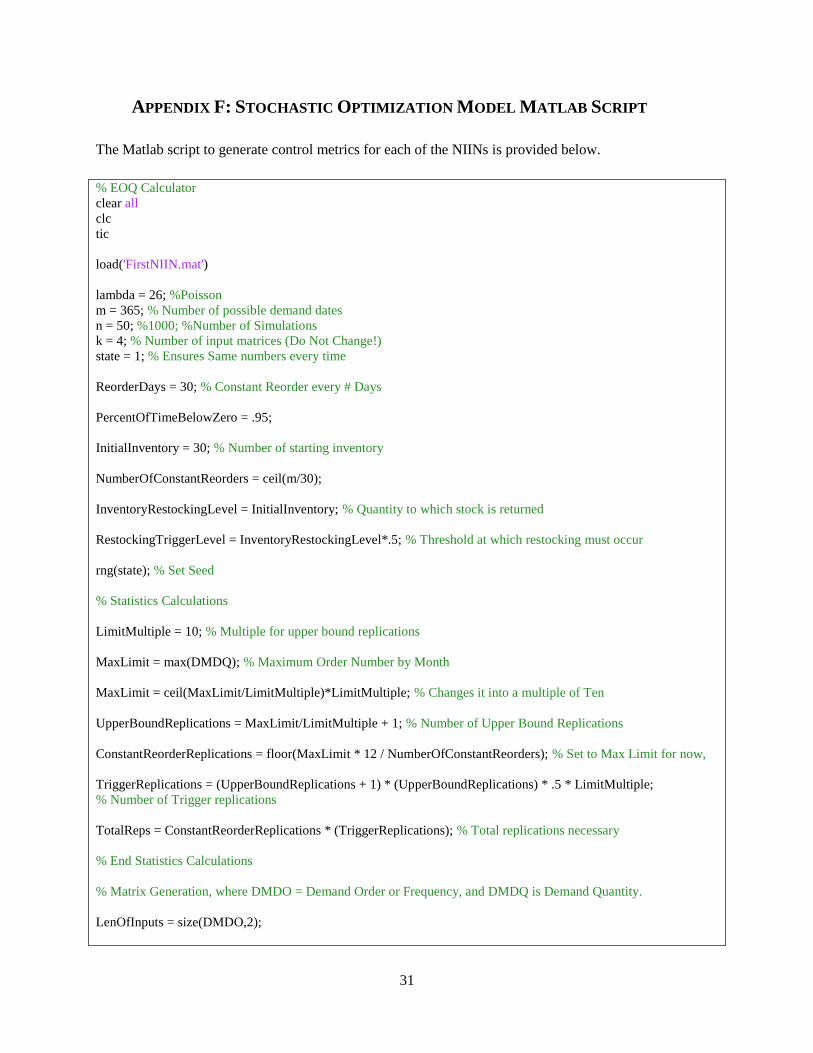
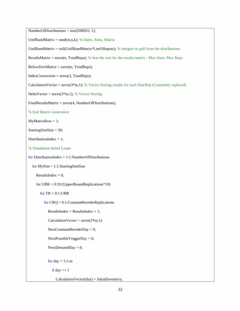
APPENDIX F: STOCHASTIC OPTIMIZATION MODEL MATLAB SCRIPT
The Matlab script to generate control metrics for each of the NIINs is provided below.
% EOQ Calculator
clear all
clc
tic
load('FirstNIIN.mat')
lambda = 26; %Poisson
m = 365; % Number of possible demand dates
n = 50; %1000; %Number of Simulations
k = 4; % Number of input matrices (Do Not Change!)
state = 1; % Ensures Same numbers every time
ReorderDays = 30; % Constant Reorder every # Days
PercentOfTimeBelowZero = .95;
InitialInventory = 30; % Number of starting inventory
NumberOfConstantReorders = ceil(m/30);
InventoryRestockingLevel = InitialInventory; % Quantity to which stock is returned
RestockingTriggerLevel = InventoryRestockingLevel*.5; % Threshold at which restocking must occur
rng(state); % Set Seed
% Statistics Calculations
LimitMultiple = 10; % Multiple for upper bound replications
MaxLimit = max(DMDQ); % Maximum Order Number by Month
MaxLimit = ceil(MaxLimit/LimitMultiple)*LimitMultiple; % Changes it into a multiple of Ten
UpperBoundReplications = MaxLimit/LimitMultiple + 1; % Number of Upper Bound Replications
ConstantReorderReplications = floor(MaxLimit * 12 / NumberOfConstantReorders); % Set to Max Limit for now,
TriggerReplications = (UpperBoundReplications + 1) * (UpperBoundReplications) * .5 * LimitMultiple;
% Number of Trigger replications
TotalReps = ConstantReorderReplications * (TriggerReplications); % Total replications necessary
% End Statistics Calculations
% Matrix Generation, where DMDO = Demand Order or Frequency, and DMDQ is Demand Quantity.
LenOfInputs = size(DMDO,2);
32
NumberOfDistributions = size(DMDO, 1);
UnifRandMatrix = rand(m,n,k); % Dates, Sims, Matrix
UnifRandMatrix = ceil(UnifRandMatrix*LenOfInputs); % Integers to pull from the distributions
ResultsMatrix = zeros(n, TotalReps); % Sets the size for the results matrix - Max Sims, Max Reps
BelowZeroMatrix = zeros(n, TotalReps);
IndexConversion = zeros(3, TotalReps);
CalculationVector = zeros(3*m,1); % Vector Storing results for each Sim/Rep (Constantly replaced)
DeltaVector = zeros(3*m,1); % Vector Storing
FinalResultsMatrix = zeros(4, NumberOfDistributions);
% End Matrix Generation
MyMatrixRow = 1;
StartingSimSize = 50;
DistributionIndex = 1;
% Simulation Initial Loops
for DistributionIndex = 1:1:NumberOfDistributions
for MySim = 1:1:StartingSimSize
ResultsIndex = 0;
for UBR = 0:10:(UpperBoundReplications*10)
for TR = 0:1:UBR
for CRQ = 0:1:ConstantReorderReplications
ResultsIndex = ResultsIndex + 1;
CalculationVector = zeros(3*m,1);
NextConstantReorderDay = 0;
NextPossibleTriggerDay = 0;
NextDemandDay = 0;
for day = 1:1:m
if day == 1
CalculationVector(day) = InitialInventory;

33
if day >= NextDemandDay
NextDemandDay = day + round(1/(DMDO(DistributionIndex, UnifRandMatrix(day, MySim,
3))*12/m));
CalculationVector(day) = CalculationVector(day) - round(DMDQ(DistributionIndex,
UnifRandMatrix(day, MySim, 2))/DMDO(DistributionIndex, UnifRandMatrix(day, MySim, 3)));
end
if day >= NextConstantReorderDay
NextConstantReorderDay = day + ReorderDays;
NextConstantReorderDelivery = day + round(ALT(DistributionIndex, UnifRandMatrix(day,
MySim, 1)) + PLT(DistributionIndex, UnifRandMatrix(day, MySim, 4)));
CalculationVector(NextConstantReorderDelivery) =
CalculationVector(NextConstantReorderDelivery) + CRQ;
end
if day >= NextPossibleTriggerDay
if CalculationVector(day) <= TR
NextTriggeredDelivery = day + round(ALT(DistributionIndex, UnifRandMatrix(day, MySim,
1)) + PLT(DistributionIndex, UnifRandMatrix(day, MySim, 4)));
NextPossibleTriggerDay = NextTriggeredDelivery;
CalculationVector(NextConstantReorderDelivery) =
CalculationVector(NextConstantReorderDelivery) + UBR - CalculationVector(day);
end
end
else
CalculationVector(day) = CalculationVector(day) + CalculationVector(day-1);
if day >= NextDemandDay
NextDemandDay = day + round(1/(DMDO(DistributionIndex, UnifRandMatrix(day, MySim,
3))*12/m));
CalculationVector(day) = CalculationVector(day) - round(DMDQ(DistributionIndex,
UnifRandMatrix(day, MySim, 2))/DMDO(DistributionIndex, UnifRandMatrix(day, MySim, 3)));
end
if day >= NextConstantReorderDay
NextConstantReorderDay = day + ReorderDays;

34
NextConstantReorderDelivery = day + round(ALT(DistributionIndex, UnifRandMatrix(day,
MySim, 1)) + PLT(DistributionIndex, UnifRandMatrix(day, MySim, 4)));
CalculationVector(NextConstantReorderDelivery) =
CalculationVector(NextConstantReorderDelivery) + CRQ;
end
if day >= NextPossibleTriggerDay
if CalculationVector(day) <= TR
NextTriggeredDelivery = day + ALT(DistributionIndex, UnifRandMatrix(day, MySim, 1)) +
PLT(DistributionIndex, UnifRandMatrix(day, MySim, 4));
NextPossibleTriggerDay = NextTriggeredDelivery;
CalculationVector(NextConstantReorderDelivery) =
CalculationVector(NextConstantReorderDelivery) + UBR - CalculationVector(day);
end
end
end
end
BelowZeroCounter = 0;
for day = 1:1:m
if CalculationVector(day) < 0
BelowZeroCounter = BelowZeroCounter + 1;
end
end
ResultsMatrix(MySim, ResultsIndex) = mean(CalculationVector(1:1:m));
BelowZeroMatrix(MySim, ResultsIndex) = BelowZeroCounter;
IndexConversion([1; 2; 3],ResultsIndex) = [UBR; TR; CRQ];
end
end
end

35
end
AverageMatrix(1,:) = mean(ResultsMatrix, 1);
AverageMatrix(2,:) = var(ResultsMatrix, 1);
AverageZero(1,:) = mean(BelowZeroMatrix, 1)/m;
ZeroBool = (le(AverageZero, 1-PercentOfTimeBelowZero)-.5)*2;
NegativeRemoval = ge(AverageMatrix(1,:).*ZeroBool, 0).*AverageMatrix(1,:) +
lt(AverageMatrix(1,:).*ZeroBool, 0)*1000;
[CurrentLegitimateMin, MinIndex] = min(NegativeRemoval);
FinalResultsMatrix(1, DistributionIndex) = CurrentLegitimateMin;
FinalResultsMatrix([2; 3; 4], DistributionIndex) = IndexConversion([1; 2; 3], MinIndex);
end
toc