www.druid.dk

DRUID Working Paper No. 09-02

Inventive Process as a Recombinant Search over Complex Landscape: Evidence from the Disk Drive Industry

By

Martin Ganco

www.druid.dk

Inventive Process as a Recombinant Search over Complex Landscape:

Evidence from the Disk Drive Industry

Martin Ganco College of Business

University of Illinois at Urbana-Champaign 350 Wohlers Hall, 1206 S. Sixth Street

Champaign, IL 61830 Voice : (217) 333-2821 Fax : (217) 244-7969

E-mail: mganco2@illinois.edu

Version : January 2009 Abstract: The inventive process has been often modeled as a bounded iterative trial-and-error recombinant search over complex landscape. Our main research question is whether such approximation is empirically valid. To investigate it, we develop a single-industry measure of invention interdependence and provide a relatively direct test of the canonical NK model. Our findings indicate that the NK model correctly predicts most of the empirical patterns. We also find that the consistency between the empirical estimates and the model predictions deteriorates with expanded definition of industry boundaries. Our results suggest that models representing iterative trial-and-error recombinant search are applicable as approximations of the inventive process when one looks at single mature industries where most of the knowledge originates from within the same technological domain. When inventors draw from a broad knowledge base and fundamentally new knowledge is created then applicability of simple models of recombinant search may be limited. Keywords: Invention, Recombinant Search, Complexity, NK Model, Simulation, Interdependence Jel codes:

ISBN 978- 87-7873-281-1

1. INTRODUCTION

Understanding what drives successful inventions became central to an eclectic body of

research. Many scholars, dating back at least to Schumpeter (1934, 1939) propose to

conceptualize inventions and innovations as novel combinations of existing resources

(Schumpeter, 1934, 1939; Penrose, 1959; Nelson and Winter, 1982; Mahoney, 1995) or

knowledge (Galunic and Rodan, 1998; Henderson and Clark, 1990). More recent work on

complex adaptive systems (Frenken, 2000, 2001a, 2001b; Fleming and Sorenson, 2001, 2004;

Ethiraj and Levinthal, 2004; Murmann and Frenken, 2006; Sorenson, Rivkin and Fleming, 2006;

Marengo, Pasquali and Valente, 2007) extends this view by focusing on the process of search for

novel combinations. By means of analogy to the concepts of mutation and recombination in

biology and to associated NK modeling framework (Kauffman, 1993, 1995), the complexity

scholars theorize that the inventions emerge from bounded, iterative, trial-and-error search for

novel combinations of existing building blocks over a complex search space.

Such conceptualization of the inventive process is theoretically appealing which is

reflected in its rising popularity among scholars (Frenken, 2000, 2001a, 2001b; Fleming and

Sorenson, 2001, 2004; Ethiraj and Levinthal, 2004; Murmann and Frenken, 2006; Sorenson et

al., 2006; Marengo et al., 2007). Nevertheless, the empirical tests of this theoretical framework

have been limited and provide mixed results. Laying important foundation, Fleming and

Sorenson (2001) empirically test some predictions of the NK model but find only partial support.

They report that some of the core predictions of the NK model are inconsistent with the data. The

authors conclude that the NK models developed primarily to approximate blind biological

evolution have limited applicability to the inventive processes – presumably because cognition

plays an important role. In support of their argument, Fleming and Sorenson (2004) find that

scientific knowledge facilitates the search for inventions as problem interdependence increases.

Notwithstanding the existing studies, the question remains open. Is modeling the

inventive process as a bounded iterative search over complex landscape a valid approximation?

If it is, what the boundary conditions of its applicability are? More specifically, can we predict

invention performance based on the empirical counterparts of the N and K model parameters? To

investigate these questions, we develop a relatively direct test of the NK model using a single

industry dataset and a new measure of technological interdependence.

To foreshadow our main results, we find that the model predictions and the empirical

estimates are consistent for the core predictions of the NK model. We also perform a

supplemental analysis which reveals that the quality of the correspondence between the model

predictions and the empirical estimates depends on how one defines the industry. Including

broader and more recent technologies seems to deteriorate the ability of the model to predict the

data. Our analysis thus highlights a contingency that modeling inventive process as an iterative

bounded search over a complex landscape can be a viable conceptualization in some settings.

2. INVENTIVE PROCESS AS A RECOMBINANT SEARCH

The application of the NK modeling framework (Kauffman, 1993, 1995; Levinthal, 1997;

Frenken, 2000, 2001a, b; Fleming and Sorenson, 2001; Rivkin, 2000, 2001; Ethiraj and

Levinthal, 2004) to the inventive process hinges on several assumptions. The problem solved by

the agent as well as the agent’s search capability is assumed to be exogenous and its properties

are controlled by simulation parameters. More specifically, the size of the solved problem

(number of components that need to be combined) and the level of interdependence (number of

interactions among components) are controlled by the parameters N and K. The inventive process

is typically performed by the trial-and-error local search (one component decision is altered at a

time) – which is either a conceptualization of the search for novel combinations of existing

knowledge (Fleming and Sorenson, 2001, 2004), search by imitation (Rivkin, 2000, 2001) or

search for new solutions (e.g. Ethiraj and Levinthal, 2001; Frenken 2001a).

The core implications of the NK model reside in the relationship between the variables N

and K and the payoff. The payoff is measured as either potentially achievable on the landscape

(i.e. the global peak) or achievable by agents on average. Prior research has shown (Kauffman,

1993, 1995; Levinthal, 1997) that higher values of interdependence (controlled by the parameter

K) create more rugged search space with higher global peak, higher potential performance but

also lead to premature lock-in called the complexity catastrophe (Kauffman, 1993). As the value

of opportunities increases with K, the landscape consists of many “peaks and valleys” and better

opportunities become on average harder to find through local search. Important role also plays

the size of the system determined by N or, more precisely, the ratio between K and N.1 With

increasing N the peaks are more spread out throughout the search space which increases maxima

since conflicting tradeoffs are less likely (a component affecting performance of more than one

other component). Consequently, increase in N attenuates the likelihood of complexity

catastrophe, increases average as well as the global peak. Since the space is easier to search, the

reward for the best, relative to the mean performance, also decreases.2 Due to potentially

1 There exists a special case of the interaction pattern when N is irrelevant for ordering of payoffs (it only affects the variance of the overall payoff distribution). In this case, only K/2 neighbor components on each side are linked, the space wraps around as a torus and K is low relative to N. 2 The majority of the existing literature within the domains of strategy and technology management assumes that the size of the solved problem N is fixed. Aside from some discussion in Kauffman (1993, 1995) the information on how N and K exactly interact is not readily available. Consequently, the purpose of the section that follows is not only to establish baseline results for the comparison with the empirical model but also disentangle the driving force behind both the performance mean and the variance of the inventive process when seen as a recombinant search over NK landscape.

different effects on the average versus the best agents, the NK model has implications not only

for the mean performance but also for its variance which necessitates analysis that looks at both.

The above imagery as well as the NK modeling apparatus has spurred many studies and

led to important insights. For instance, Ethiraj and Levinthal (2004) study how underlying

technological modularity interacts with design in its effect on performance. Murmann and

Frenken (2006) theorize how innovations and dominant designs emerge over time and Frenken

(2001a) suggests how modularity changes with industry life-cycle. Further studies look at the

link between organizational attributes and technological problem solving (e.g. Marengo et al.,

2007; Rivkin and Siggelkow, 2007).

As we maintain, the more fundamental question is whether the NK model is a valid

approximation of the inventive process. The only study to date that tackled this issue explicitly

was by Fleming and Sorenson (2001) who laid an important groundwork for resolving it. The

authors hypothesize and test some of the predictions of the NK model. Importantly, Fleming and

Sorenson (2001) found no support for the core prediction that the performance in rugged

landscapes is driven by the interaction between the N and K attributes. The authors build a

measure of technological interdependence by looking at a cross-section of issued patents -

implicitly assuming that knowledge is drawn from wide contexts and that the nature of

interdependencies remains stable across industry boundaries.

To revisit the issue of whether and when the NK model approximates the inventive

process, we take the following approach: first, we simulate the basic NK model and use

regression analysis to obtain predicted values of performance as a function of the N and K

parameters. We then carry out a similar analysis empirically by developing measures of N and K

and performing regression on a single-industry dataset. We then conclude by comparing the two

sets of predicted values.

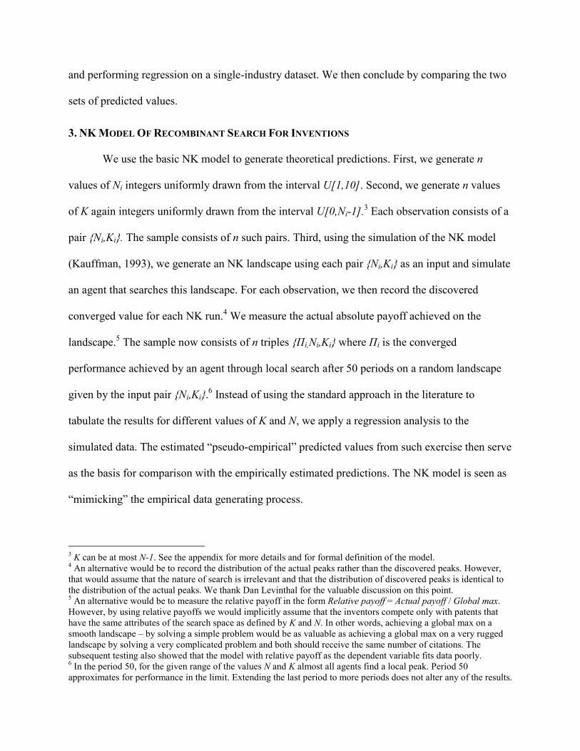
3. NK MODEL OF RECOMBINANT SEARCH FOR INVENTIONS

We use the basic NK model to generate theoretical predictions. First, we generate n

values of Ni integers uniformly drawn from the interval U[1,10]. Second, we generate n values

of K again integers uniformly drawn from the interval U[0,Ni-1].3 Each observation consists of a

pair {Ni,Ki}. The sample consists of n such pairs. Third, using the simulation of the NK model

(Kauffman, 1993), we generate an NK landscape using each pair {Ni,Ki} as an input and simulate

an agent that searches this landscape. For each observation, we then record the discovered

converged value for each NK run.4 We measure the actual absolute payoff achieved on the

landscape.5 The sample now consists of n triples {Πi,Ni,Ki} where Πi is the converged

performance achieved by an agent through local search after 50 periods on a random landscape

given by the input pair {Ni,Ki}.6 Instead of using the standard approach in the literature to

tabulate the results for different values of K and N, we apply a regression analysis to the

simulated data. The estimated “pseudo-empirical” predicted values from such exercise then serve

as the basis for comparison with the empirically estimated predictions. The NK model is seen as

“mimicking” the empirical data generating process.

3 K can be at most N-1. See the appendix for more details and for formal definition of the model. 4 An alternative would be to record the distribution of the actual peaks rather than the discovered peaks. However, that would assume that the nature of search is irrelevant and that the distribution of discovered peaks is identical to the distribution of the actual peaks. We thank Dan Levinthal for the valuable discussion on this point. 5 An alternative would be to measure the relative payoff in the form Relative payoff = Actual payoff / Global max. However, by using relative payoffs we would implicitly assume that the inventors compete only with patents that have the same attributes of the search space as defined by K and N. In other words, achieving a global max on a smooth landscape – by solving a simple problem would be as valuable as achieving a global max on a very rugged landscape by solving a very complicated problem and both should receive the same number of citations. The subsequent testing also showed that the model with relative payoff as the dependent variable fits data poorly. 6 In the period 50, for the given range of the values N and K almost all agents find a local peak. Period 50 approximates for performance in the limit. Extending the last period to more periods does not alter any of the results.

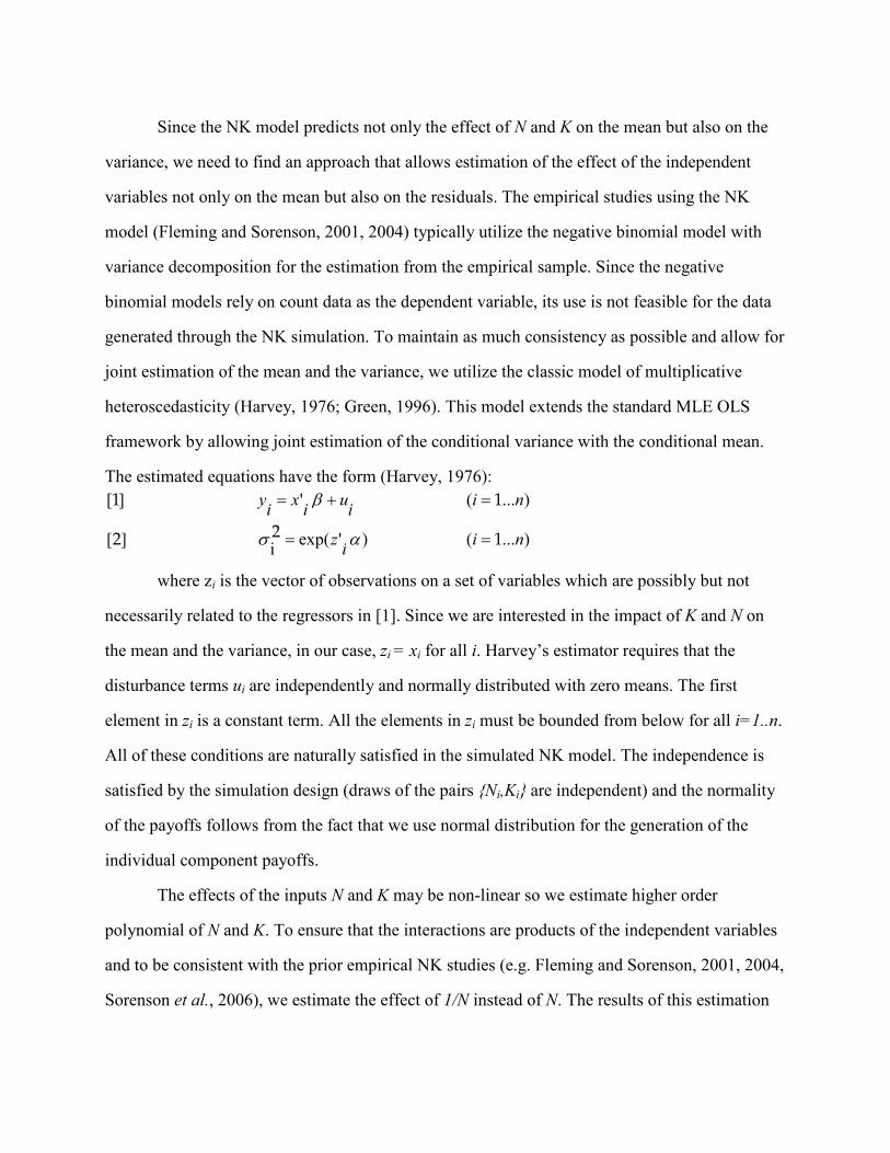
Since the NK model predicts not only the effect of N and K on the mean but also on the

variance, we need to find an approach that allows estimation of the effect of the independent

variables not only on the mean but also on the residuals. The empirical studies using the NK

model (Fleming and Sorenson, 2001, 2004) typically utilize the negative binomial model with

variance decomposition for the estimation from the empirical sample. Since the negative

binomial models rely on count data as the dependent variable, its use is not feasible for the data

generated through the NK simulation. To maintain as much consistency as possible and allow for

joint estimation of the mean and the variance, we utilize the classic model of multiplicative

heteroscedasticity (Harvey, 1976; Green, 1996). This model extends the standard MLE OLS

framework by allowing joint estimation of the conditional variance with the conditional mean.

The estimated equations have the form (Harvey, 1976):

)...( )'exp(i ][

)...( ' ][

niiz

niiuixiy

122

11

==

=+=

ασ

β

where zi is the vector of observations on a set of variables which are possibly but not

necessarily related to the regressors in [1]. Since we are interested in the impact of K and N on

the mean and the variance, in our case, zi = xi for all i. Harvey’s estimator requires that the

disturbance terms ui are independently and normally distributed with zero means. The first

element in zi is a constant term. All the elements in zi must be bounded from below for all i=1..n.

All of these conditions are naturally satisfied in the simulated NK model. The independence is

satisfied by the simulation design (draws of the pairs {Ni,Ki} are independent) and the normality

of the payoffs follows from the fact that we use normal distribution for the generation of the

individual component payoffs.

The effects of the inputs N and K may be non-linear so we estimate higher order

polynomial of N and K. To ensure that the interactions are products of the independent variables

and to be consistent with the prior empirical NK studies (e.g. Fleming and Sorenson, 2001, 2004,

Sorenson et al., 2006), we estimate the effect of 1/N instead of N. The results of this estimation

where integers N are drawn from U[1,10] and K from U[0,N-1] are reported in Table 1.7 The

models differ by the degree of polynomial. We have estimated the model up to the fifth degree

polynomial though only the first three are reported.8 The estimation is implemented as reghv

procedure in Stata. The regression results are shown in Table 1.

[Insert Table 1 about here]

Clearly, the effects of N and K on the payoffs are highly non-linear. Although almost all

of the coefficients are statistically significant, it is evident that the coefficients on the interaction

terms are important in determining the payoffs. This holds even as we take into account different

magnitudes of the underlying variables (i.e. K is between 0 and 9 and K/N between 0 to 0.9). For

instance, at N=3 and change in K from 0 to 1, the impact of the interaction terms on the payoff is

3.93 times larger than the effect of the coefficients on K and K2. It implies that the payoffs in the

NK model are driven by a delicate interplay between the N – size of the problem being solved

and K – the number of linkages among the problem components.

Complementing the regression results in Table 1, predicted values for the mean and the

variance as a function of N and K are shown in Figures 1-6. Figure 3 shows increase in N for

fixed K. With increasing problem size the peaks spread out over a larger space and conflicting

tradeoffs are less likely which improves mean performance. However, this occurs at a decreasing

rate since as N gets large relative to K it is increasingly unlikely that a single component affects

performance of more than one other component.

Higher value of K implies higher global maxima but also more rugged landscape and

increased potential for lock-in. More dense linkages between the invention components lead to

better opportunities but also create difficulties in their exploitation. Nevertheless, the K value

itself has smaller direct impact on the actual discovered payoffs than the interplay between the K

7 The predicted values were generated using the specific values of N and K. However, we have verified that the qualitative pattern of the predicted effects as discussed below is robust to all admissible values of the model parameters. 8 We have also tried to include cross products of all terms. Despite some of the coefficients - especially for the variance portion of the model - are significant their magnitude is very small and they do not seem to change the nature of the predicted effects. We omit them for the sake of simplicity and estimation power.

and N since an increase in N mitigates the impact of a rugged landscape. For low values of K/N,

as K/N increases (Figure 1), the agent is able to exploit the increasing payoff of local peaks since

high relative N allows better fine-tuning of the solution due to lower likelihood of conflicting

trade-offs. However, this occurs at a decreasing rate since increasing K for fixed N increases

number of linkages and the likelihood that they will be conflicting (a single component choice

affecting multiple other components for a given K and N) which rapidly increases chances of

lock-in and eventually leads to decline in the payoffs as K/N goes to 1.

The case with K/N fixed and changing both N and K shows similar non-linearity (Figure

5). In this case, the pattern is driven by the coefficients on the terms 1/N and K. As N and K

increase, the performance again increases though at a decreasing rate as it is the case with the

fixed K. The marginal benefit of having larger space outweighs the costs of increases in K since

the coefficients on K are small.9

Although the interpretation of the variance portion of the estimated model is less

straightforward, the results show that the variance is non-linear and driven by all components -

N, K, the interaction terms K/N and their higher order terms (Table 1). It is also notable that the

variance decreases for all cases and at a decreasing rate (Figure 2, 4, 6). The intuition behind this

result is that increases in K/N make differences across landscapes less random (Figure 2). The

average payoff achieved on a more rugged landscape will be similar across landscapes since all

will exhibit similar lock-in problems. Within landscape the differences may very well increase

with K/N as higher K makes distribution of payoffs within landscape more dispersed. The

increasing within landscape differences contribute to the decreasing rate at which across

landscape differences decrease. However, the across landscape effect dominates.10 Increasing N

(Figure 4) lowers variance by allowing easier search through smoother space and decreasing

both the within and across landscape variation. This is again at decreasing rate since higher N

9 For instance, with K = 1 and N = 2 the probability that the focal component does not affect any other component beyond itself is 0. For K = 2 and N = 4, this probability increases to 1/27. Even for fixed K/N the likelihood of conflicting tradeoffs decreases. 10 If we would measure the relative payoffs instead of the actual payoffs the variance would increase with K/N.

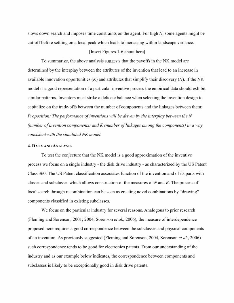
slows down search and imposes time constraints on the agent. For high N, some agents might be

cut-off before settling on a local peak which leads to increasing within landscape variance.

[Insert Figures 1-6 about here]

To summarize, the above analysis suggests that the payoffs in the NK model are

determined by the interplay between the attributes of the invention that lead to an increase in

available innovation opportunities (K) and attributes that simplify their discovery (N). If the NK

model is a good representation of a particular inventive process the empirical data should exhibit

similar patterns. Inventors must strike a delicate balance when selecting the invention design to

capitalize on the trade-offs between the number of components and the linkages between them:

Proposition: The performance of inventions will be driven by the interplay between the N

(number of invention components) and K (number of linkages among the components) in a way

consistent with the simulated NK model.

4. DATA AND ANALYSIS

To test the conjecture that the NK model is a good approximation of the inventive

process we focus on a single industry - the disk drive industry - as characterized by the US Patent

Class 360. The US Patent classification associates function of the invention and of its parts with

classes and subclasses which allows construction of the measures of N and K. The process of

local search through recombination can be seen as creating novel combinations by “drawing”

components classified in existing subclasses.

We focus on the particular industry for several reasons. Analogous to prior research

(Fleming and Sorenson, 2001; 2004, Sorenson et al., 2006), the measure of interdependence

proposed here requires a good correspondence between the subclasses and physical components

of an invention. As previously suggested (Fleming and Sorenson, 2004, Sorenson et al., 2006)

such correspondence tends to be good for electronics patents. From our understanding of the

industry and as our example below indicates, the correspondence between components and

subclasses is likely to be exceptionally good in disk drive patents.

Our measure also requires stability across observations (the functional nature of

components classified in a particular subclass needs to be relatively stable) which necessitates

single and, as we explain below, relatively narrow industry focus. The Class 360 covers only

magnetic storage (Dynamic Magnetic Information Storage or Retrieval) which provides a narrow

and well-defined industry definition. Industry, as defined by this class, is also in its very mature

stage. It implies that most of the important inventions have been undertaken and exhaustive ex-

post analysis with “self-contained” data can be performed. It is also convenient that the patents

classified in a single patent class well represent the disk drive-related patents introduced by firms

operating within the industry (Hoetker and Agarwal, 2007).

Our main interdependence measure is based on 30,861 patents classified in Class 360

between 1972 and 2004 and 18,015 prior to 1999 are used in the estimation. The patents issued

in the last 5 years of the sample are excluded from the estimation to consistently measure

citations over 5-year period following the patent issue. To empirically test the NK model, we

start with the empirical framework from prior studies (Fleming and Sorenson, 2001, 2004) and

then extend it by developing additional controls and verifying its robustness to alternative model

specifications.

4.1. DEPENDENT VARIABLE

We measure patent performance by the number of citations patent receives in the first 5

years post patent issuing date - i.e. the citing patent application date must be no later than 5 years

after the cited patent issue date. As a result, patents in the last 5 years of the industry data are not

used in the estimation as independent variables.11 Since the main objective of the citation counts

is to obtain a proxy for the general patent usefulness or performance (Trajtenberg, 1990; Hall et

al., 2000; Fleming and Sorenson, 2001) we use citations from all patents and not just from the

ones classified in the class 360. Restricting the citations only to within industry citations would

bias the measure toward the patents with narrow applicability and reduce variability in the

11 The results are robust to different specifications of this time window (4 vs. 6 years).

dependent variable. Nevertheless, we have confirmed that restricting citations only to the within-

industry citations has no effect on the shape of the predicted values of the model.12

4.2. INDEPENDENT VARIABLES

4.2.1. N: NUMBER OF COMPONENTS

Consistent with prior studies (Fleming and Sorenson, 2001, 2004; Sorenson et al., 2006),

we operationalize the number of components by the number of subclasses. The estimation and

testing of the NK model requires good correspondence between the physical components (or

“chunks of knowledge”, Sorenson et al., 2006) and patent subclasses. The focus on the disk drive

industry was partly motivated by expectation of a good correspondence. We include the number

of components in the form 1/N to reflect the fact that the interaction should be a product of two

independent variables.

4.2.2. LEVEL OF INTERDEPENDENCE K

One of the contributions of the current paper is to construct and test a new single-industry

measure of technological interdependence K. Our measure of interdependence is based on a

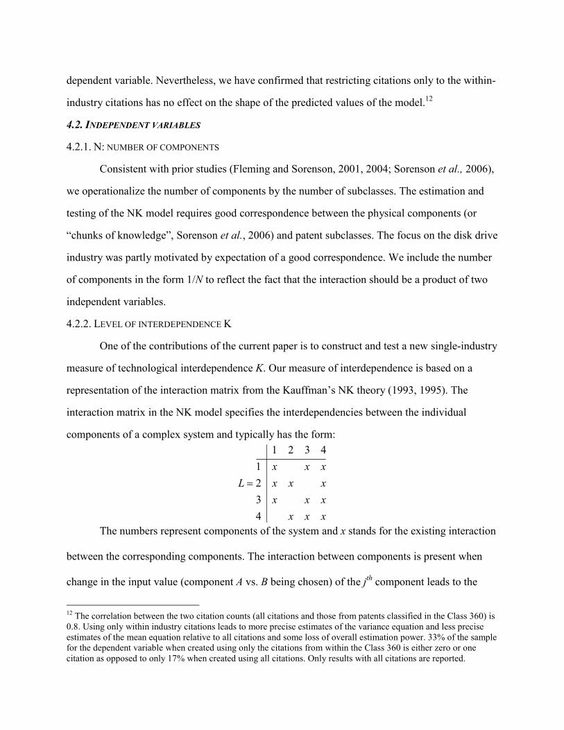
representation of the interaction matrix from the Kauffman’s NK theory (1993, 1995). The

interaction matrix in the NK model specifies the interdependencies between the individual

components of a complex system and typically has the form:

xxx

xxx

xxx

xxx

L

4

3

2

1

4321

=

The numbers represent components of the system and x stands for the existing interaction

between the corresponding components. The interaction between components is present when

change in the input value (component A vs. B being chosen) of the jth component leads to the

12 The correlation between the two citation counts (all citations and those from patents classified in the Class 360) is 0.8. Using only within industry citations leads to more precise estimates of the variance equation and less precise estimates of the mean equation relative to all citations and some loss of overall estimation power. 33% of the sample for the dependent variable when created using only the citations from within the Class 360 is either zero or one citation as opposed to only 17% when created using all citations. Only results with all citations are reported.

change in the payoff of the ith component. The model assumes that the underlying functional

structure of the system is exogenous and agents optimize it by selecting (or designing)

appropriate functional components. An x along the diagonal indicate that payoff of each

component depends on its own design or choice. Then, typically rows are influenced by columns

so x in the first row and third column indicates that the payoff contribution of the first component

is affected by the design or choice of the third component.13 The matrix above is a case with N =

4 and K = 2.14

As opposed to the binary interactions in the NK model, we estimate the amount of

interaction in each “cell” of the interaction matrix. For each component, we estimate the amount

of interaction it has with all other components. The K associated with the component i, Ki is the

sum of interactions the focal component has with all other components. Interdependence K of an

invention is then an average of the individual component Ki’s.

The key idea behind the measure is that when two underlying functions (represented by

patent subclasses) are coupled we are more likely to observe components belonging to these

subclasses in a single invention. If there is a high coupling between the functions A and B and the

component a is classified in patent subclass A, a∈A and b is in B, b∈B (USPTO classifies

patents into subclasses by its functions), then we are more likely to encounter components a and

b appearing on a patent together. In other words, high interdependence between A and B implies

that whenever inventor solves a problem related to one of these functions she needs to redesign

or include the coupled function as well and we are likely to observe the components optimizing

these functions together in a patent. Similarly, if the patent improves architecture of multiple

functions we are likely to observe all components that correspond to these functions coupled to

13 The overall system payoff in the NK model is determined by the mean of the payoff contributions of the individual components. See the technical appendix for more details. 14 The K does not include the interaction with itself.

the architecture. On the other hand, if A and B are modular with respect to each other (have no

interdependence or only interdependence through standardized interfaces), we are likely to

observe A combined with other subclasses without B being present.

It is important to note that such inference of interdependence is context-specific which

necessitates our core assumption that knowledge is sourced primarily from the same industry.

For instance, the interdependence of the “metal thin film magnetic layer” with other components

may be very high within the disk drive patents but not necessarily outside of this set. Whenever

this subclass appears on a disk drive patent it is more likely to appear with subclasses

representing “recording head” or “disk surface”. Consistent with intuition, the interdependence

between the disk surface, material of the disk surface and the recording head is high.15 However,

within a broader knowledge context such inference of interdependence may be incorrect as the

function may be industry-specific. The subclass “metal thin film magnetic layer” may recombine

with a wide variety of subclasses when one looks across industries leading to inference of high

modularity. The necessity of a stable functional context requires focus on a single industry and

self-contained patent data set.

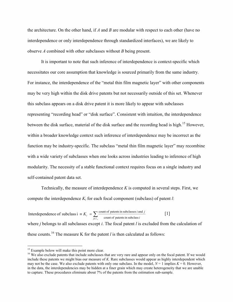
Technically, the measure of interdependence K is computed in several steps. First, we

compute the interdependence Ki for each focal component (subclass) of patent l:

∑−∈

=≡ilj

ii

ji K

subclass in patentsofcount

and subclasses in patentsofcount i subclass of denceInterdepen [1]

where j belongs to all subclasses except i. The focal patent l is excluded from the calculation of

these counts.16 The measure K for the patent l is then calculated as follows:

15 Example below will make this point more clear. 16 We also exclude patents that include subclasses that are very rare and appear only on the focal patent. If we would include these patents we might bias our measure of K. Rare subclasses would appear as highly interdependent which may not be the case. We also exclude patents with only one subclass. In the model, N = 1 implies K = 0. However, in the data, the interdependencies may be hidden at a finer grain which may create heterogeneity that we are unable to capture. These procedures eliminate about 7% of the patents from the estimation sub-sample.

∑∈

=≡li

il K Kll patent of subclasses ofcount

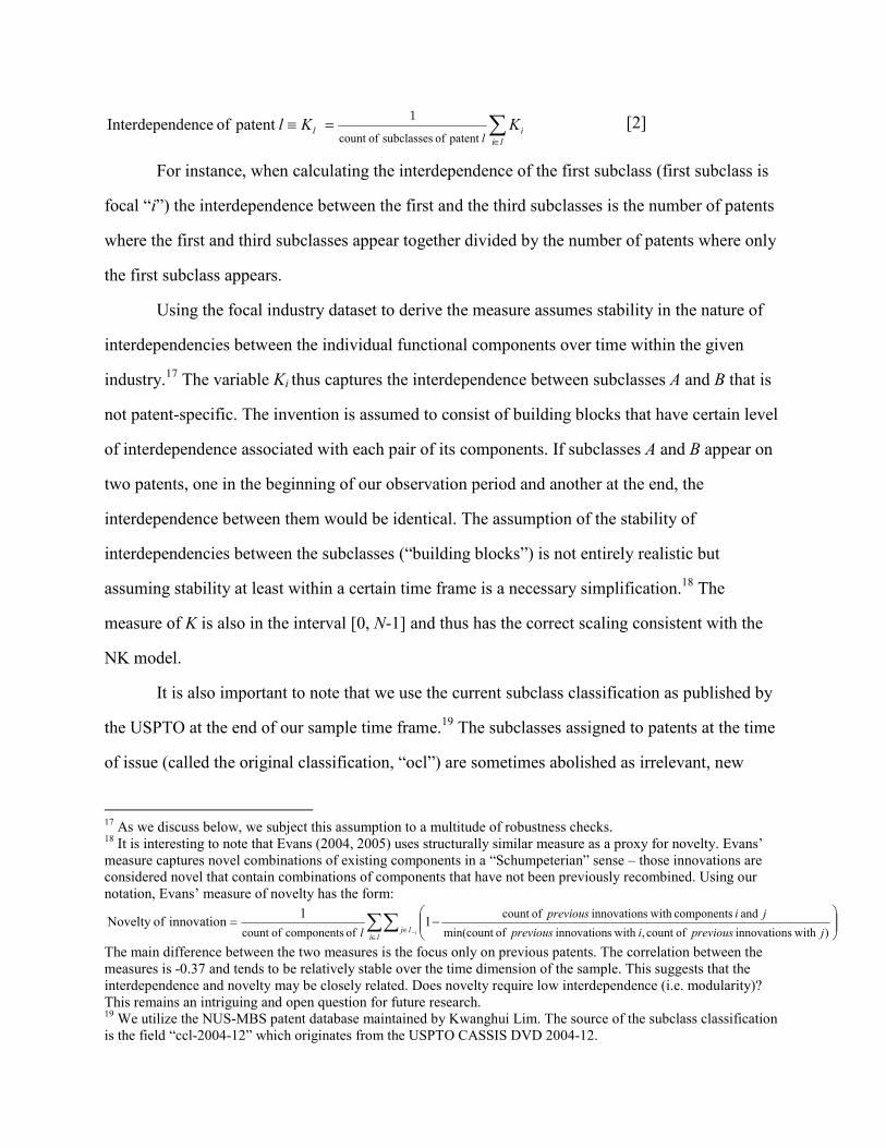
patent of denceInterdepen1 [2]

For instance, when calculating the interdependence of the first subclass (first subclass is

focal “i”) the interdependence between the first and the third subclasses is the number of patents

where the first and third subclasses appear together divided by the number of patents where only

the first subclass appears.

Using the focal industry dataset to derive the measure assumes stability in the nature of

interdependencies between the individual functional components over time within the given

industry.17 The variable Ki thus captures the interdependence between subclasses A and B that is

not patent-specific. The invention is assumed to consist of building blocks that have certain level

of interdependence associated with each pair of its components. If subclasses A and B appear on

two patents, one in the beginning of our observation period and another at the end, the

interdependence between them would be identical. The assumption of the stability of

interdependencies between the subclasses (“building blocks”) is not entirely realistic but

assuming stability at least within a certain time frame is a necessary simplification.18 The

measure of K is also in the interval [0, N-1] and thus has the correct scaling consistent with the

NK model.

It is also important to note that we use the current subclass classification as published by

the USPTO at the end of our sample time frame.19 The subclasses assigned to patents at the time

of issue (called the original classification, “ocl”) are sometimes abolished as irrelevant, new

17 As we discuss below, we subject this assumption to a multitude of robustness checks. 18 It is interesting to note that Evans (2004, 2005) uses structurally similar measure as a proxy for novelty. Evans’ measure captures novel combinations of existing components in a “Schumpeterian” sense – those innovations are considered novel that contain combinations of components that have not been previously recombined. Using our notation, Evans’ measure of novelty has the form:

∑∑∈

∈ −

−=

lilj i jpreviousiprevious

jiprevious

l ) with sinnovation ofcount , with sinnovation ofmin(count

and components with sinnovation ofcount

of components ofcount 1

1innovation of Novelty

The main difference between the two measures is the focus only on previous patents. The correlation between the measures is -0.37 and tends to be relatively stable over the time dimension of the sample. This suggests that the interdependence and novelty may be closely related. Does novelty require low interdependence (i.e. modularity)? This remains an intriguing and open question for future research. 19 We utilize the NUS-MBS patent database maintained by Kwanghui Lim. The source of the subclass classification is the field “ccl-2004-12” which originates from the USPTO CASSIS DVD 2004-12.

classes are created (24% of the patents in our sample have at least one subclass that is subject to

reclassification) and patents are reclassified. We believe that the current classification is more

precise since it is more likely to represent same functional components in different patents by the

same subclass. However, as we show below, we have verified that our results are fully robust to

whether we use the original or the current classification.20

To highlight the mechanics of the measure, it may be instrumental to discuss an example

(Table 2). The patent #5,949,612 “Low friction sliding hard disk drive system” was classified

into the following subclasses (the subclasses are listed with the calculated values of Ki).21 Figure

7 provides the description of patent from the first page of the patent document.

[Insert Table 2 and Figure 7 about here]

We may note that the most interdependent classes in the above patent are the “stock

material” subclasses 428. Within the context of the main class 360, the “material” subclasses

typically represent the surface of the rotating disk or material of the reading head. The functional

context of these subclasses tends to be the same across many patents. Whenever the “stock

material” subclass appears on the patent, it is more likely that the subclass representing the disk

or the head appears as well, suggesting interdependence.

It is also illustrative to look at how the measure orders the patents within the industry. If

we order the patents according to K/N, the patents range from K/N = 0 to K/N = 0.704 with the

mean of 0.077 and the median of 0.062. The patents with higher values of K/N are typically those

that solve specific design and method issues of the disks mounting, disk surface, head design or

application specific issues of the tape handling mechanism - loading, reeling, etc. Around the

mean value tend to be inventions addressing more systemic issues like data processing, mounting

structures, cartridge design issues, etc. Among the least interdependent inventions are those that

deal with methods of data processing, memory design issues, wiring and grounding of the

systems, controllers, signal filters, etc. As an interesting extreme example, one of the patents

20 We thank Mu-Yen Hsu for a valuable discussion on this issue. 21 The patent has received 24 citations.

with a very low K/N is an IBM patent 5,953,180 describing different markings of the disk

assembly mechanism.

4.3. CONTROL VARIABLES

When inventors file patent applications they do so in anticipation of economic returns –

supposedly in a technological area where they expect such returns to be the greatest.

Consequently, the distribution of patents across subclasses is not random which creates an

endogeneity problem that needs to be addressed. The approach that we adopt is to include a set

of proxy variables that should control for unobserved differences potentially driving the results

as well as employ a host of robustness checks using alternative measures and model

specifications.

4.3.1. TECHNOLOGY CONTROLS From the perspective of the above endogeneity problem, the main concern with the

proposed measure of technological interdependence is that it relies on relative frequency counts

for the inference of interdependence. Inventors are more likely to patent in attractive

technological areas so attractiveness (unrelated to interdependence) in a certain domain may

affect both the frequency ratios used to measure K as well as citations. The objective of some of

the controls is thus to proxy for the general attractiveness of a given technological area.

Prior studies have tackled this issue by introducing the technology mean and variance

controls (Fleming and Sorenson, 2001, 2004). We utilize similar approach but we add several

additional controls complementing those used in prior research. The technology mean control

has the form:

∑

∑

=≡

=≡ ∈

i iill

ij j

i

pMl

ij i

µ

µ

for patent control mean Technology

class in patentsofcount

citations Class in Citations Average [3]

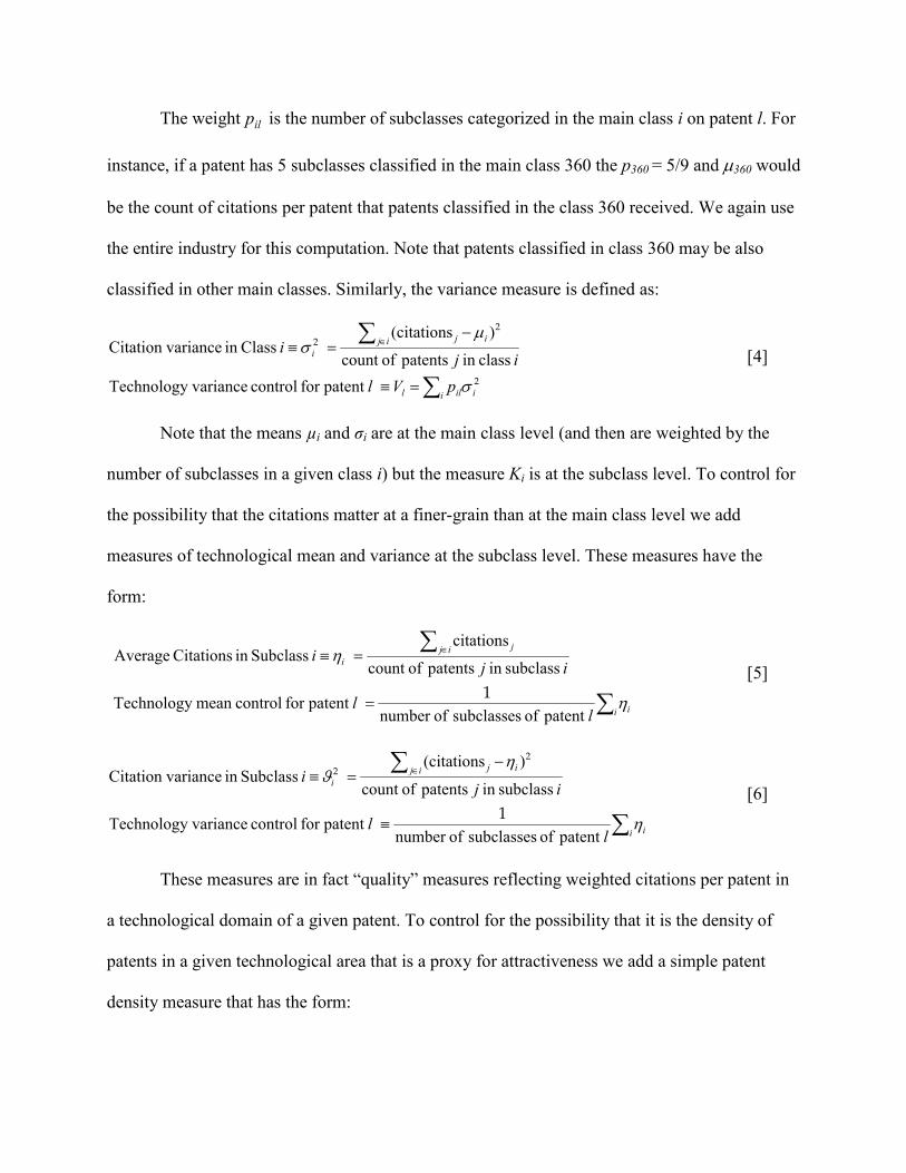
The weight ilp is the number of subclasses categorized in the main class i on patent l. For

instance, if a patent has 5 subclasses classified in the main class 360 the p360 = 5/9 and µ360 would

be the count of citations per patent that patents classified in the class 360 received. We again use

the entire industry for this computation. Note that patents classified in class 360 may be also

classified in other main classes. Similarly, the variance measure is defined as:

∑

∑

=≡

−=≡ ∈

i iill

ij ij

i

pVl

ij i

2

22

σ

µσ

for patent control variance Technology

class in patentsofcount

)(citations Class in variance Citation [4]

Note that the means µi and σi are at the main class level (and then are weighted by the

number of subclasses in a given class i) but the measure Ki is at the subclass level. To control for

the possibility that the citations matter at a finer-grain than at the main class level we add

measures of technological mean and variance at the subclass level. These measures have the

form:

∑

∑

=

=≡ ∈

i i

ij j

i

ll

ij i

η

η

patent of subclasses ofnumber for patent control mean Technology

subclass in patentsofcount

citations Subclass in Citations Average

1 [5]

∑

∑

≡

−=≡ ∈

i i

ij ij

i

ll

ij i

η

ηϑ

patent of subclasses ofnumber for patent control variance Technology

subclass in patentsofcount

)(citations Subclass in variance Citation

1

22

[6]

These measures are in fact “quality” measures reflecting weighted citations per patent in

a technological domain of a given patent. To control for the possibility that it is the density of

patents in a given technological area that is a proxy for attractiveness we add a simple patent

density measure that has the form:

∑=i

il

l subclass in patentsofcount of subclasses ofnumber

for patent control densityPatent 1 [7]

4.3.2. PRIOR ART CITATION

The prior art citations - in the form of the number of references made by the focal patent -

control for the localness of search and propensity to patent (Fleming and Sorenson, 2001).

Building more on the existing patents suggests that the inventor searches in the neighborhood of

the existing knowledge (Podolny and Stuart, 1995) as opposed to looking for truly novel

knowledge. The propensity to be cited correlates with the number of citations patent makes on

average and thus the number of citations a focal patent makes may capture “idiosyncratic

differences in patenting activity that [the] class controls miss” (Fleming and Sorenson, 2001).

4.3.3. NUMBER OF CLASSES

Consistent with the logic described in prior studies (Fleming and Sorenson, 2001, 2004),

higher number of main classes may mean broader applicability and relevance of the patent for

subsequent innovations. The patents with more classes may be also more at risk for subsequent

citations simply because they happen to be in the same class as the subsequent patent.

4.3.4. NUMBER OF TRIALS The number of prior trials measures the number of times a particular combination of

subclasses has been used before (Fleming and Sorenson, 2001; 2004). It serves to capture the

number of peaks that have been already found and search limitations associated with the

exhaustion of combinatorial possibilities. Using this control should capture the pre-emption or

crowding out - factors that likely affect citation patterns.

4.3.5. TIME DUMMIES AND INVENTOR FIXED EFFECTS

We add time dummies to all regressions as a way of capturing changes in citation

patterns over time.

Using matching algorithm described in Agarwal et al. (2009) we also match inventor

names to create unique inventor identifiers. To control for unobserved heterogeneity at the

individual inventor level we run the models also using the inventor fixed-effects. Since on

average each patent lists multiple inventors using inventor fixed-effects changes sample

structure. Instead of an observation being a patent it becomes an inventor-patent with an increase

in the sample size. For this reason, we report the fixed-effects models as a robustness check.

The descriptive statistics of the sample are provided in Table 3.

4.4. REGRESSION MODELS

We adopt the estimation technique from prior studies (Fleming and Sorenson, 2001,

2004) but we test its robustness using alternative specifications. Since it is necessary to estimate

both the variance and the mean (ideally jointly) on a data with a count dependent variable, the

choice of an estimation method is relatively limited. Ideally, we would like to use a method that

is fully equivalent to the multiplicative heteroscedasticity model used in the estimation of the

theoretical model. Since the dependent variable in the NK model is normally distributed and we

use non-normally distributed citation counts as the dependent variable in the empirical model,

clean use of the same model specification on both sets of data is not possible. Using the

multiplicative heteroscedasticity model on count data violates the normality assumption

necessary for consistent estimates using maximum likelihood.

For the joint estimation of the variance and mean of the citation count data we use the

Negbin II specification (Cameron and Trivedi, 1986) of the negative binomial regression as the

main model. This specification allows joint maximum likelihood estimation of the mean and the

dispersion parameter α conditional on the exogenous regressors (STATA implements this routine

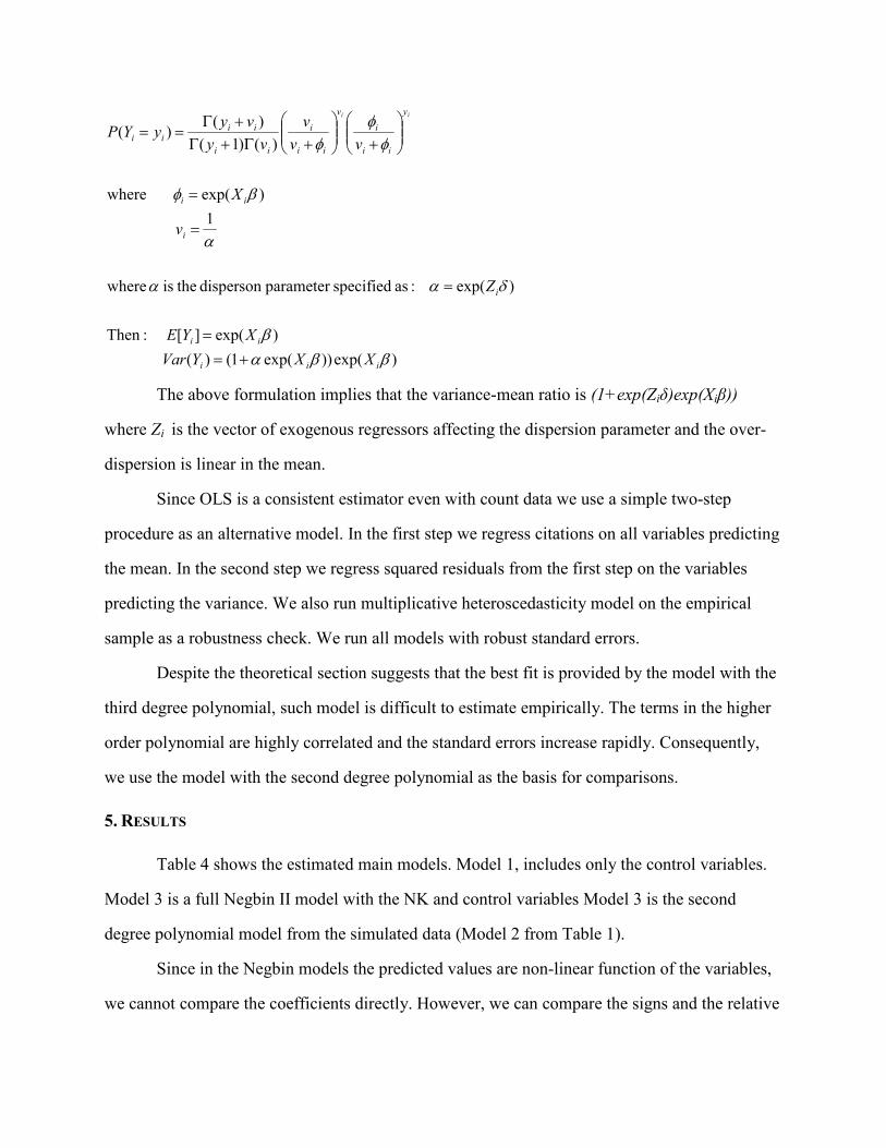
as gnbreg). The Negbin II model has the form:

)exp())exp(1()(

)exp(][ :Then

)exp( :as specified parameterdisperson theis where

1

)exp( where

)()1()(

)(

ββαβ

δαα

α

βφ

φφ

φ

iii

ii

i

i

ii

y

ii

i

v

ii

i

ii

iiii

XXYVar

XYE

Z

v

X

vvv

vyvy

yYPii

+=

=

=

=

=

+

+Γ+Γ+Γ

==

The above formulation implies that the variance-mean ratio is (1+exp(Ziδ)exp(Xiβ))

where Zi is the vector of exogenous regressors affecting the dispersion parameter and the over-

dispersion is linear in the mean.

Since OLS is a consistent estimator even with count data we use a simple two-step

procedure as an alternative model. In the first step we regress citations on all variables predicting

the mean. In the second step we regress squared residuals from the first step on the variables

predicting the variance. We also run multiplicative heteroscedasticity model on the empirical

sample as a robustness check. We run all models with robust standard errors.

Despite the theoretical section suggests that the best fit is provided by the model with the

third degree polynomial, such model is difficult to estimate empirically. The terms in the higher

order polynomial are highly correlated and the standard errors increase rapidly. Consequently,

we use the model with the second degree polynomial as the basis for comparisons.

5. RESULTS

Table 4 shows the estimated main models. Model 1, includes only the control variables.

Model 3 is a full Negbin II model with the NK and control variables Model 3 is the second

degree polynomial model from the simulated data (Model 2 from Table 1).

Since in the Negbin models the predicted values are non-linear function of the variables,

we cannot compare the coefficients directly. However, we can compare the signs and the relative

effect in the mean portion of the model since exp(.) is a monotonic transformation. The

correspondence between the coefficients as well as the predicted values (Figures 8, 10, 12) of the

mean portion between the empirical and the theoretical model is strong.22 The empirical

estimation also correctly captures smaller direct effect of the interdependence K and its square

term K2 and stronger and significant effect of its interactions with N. For instance, at N = 3 and a

change from K = 0 to K = 1 the effect of interaction term coefficients on citations is twice as

large as that of the coefficients on K and K2. Empirical analysis thus supports the prediction of

the model that even as the level of interdependence determines the nature of the landscape what

matters for performance is the interplay between the interdependence and the number of

components. The effects of the interdependence and the number of components cannot be

analyzed in isolation.

Overall, the effects of K and N and their interaction terms are relatively large. For

example, for N = 3, deviating from the mean level of K/N by one standard deviation increases the

citations on average by about 0.5. As the inverted U-shaped relationship in Figure 8 and the

concave and increasing relationship in Figure 10 suggest, we find a strong support for the

complexity catastrophe (Kauffman, 1993, 1995). The complexity catastrophe implies that the

penalty for interdependence will be strongest when K is close to N for small N. Also we find that

at fixed K, increasing N improves performance but at a decreasing rate - consistent with the NK

model. Overall, the mean estimation of the empirical model captures the attributes of the

simulated NK model relatively well.

The theoretical model predicts the optimum level of K/N* = 0.42 (at the median of the

simulated data of N = 5). The estimated model puts this level at K/N*est = 0.19 (at the empirical

median of N = 3). This difference could result from the fact that we are unable to capture some

interdependencies and our estimates of K and N are low estimates.23 Interestingly, the optimal 22 The figures are created as following: the value which is fixed is at the 50th percentile in the empirical sample and the x axis starts and ends at the 5th and 95th percentiles, respectively. For instance, in Figure 8, the N is fixed at 3 which is the median of the sample and the x axis starts at K = 0 (5th percentile) and ends at K = 1 (95th percentile). 23 Due to the noise in the measures and limitations associated with the patent data, the comparisons like these need to be taken with caution.

level of K/N*est is about 87th percentile in the empirical sample (95th percentile is 0.25). It

indicates that there are very few patents with truly high interdependence and that the majority of

the issued patents are very modular.24

On the other hand, the results of the variance portion of the model are statistically weaker

(Figure 9, 11, 13) and tend to be inconsistent with the NK model. The most notable difference is

that the estimated variance tends to closely scale with the mean. This could happen for several

reasons. First, the precision of the measure of interdependence K may decrease with K. Since

patent interdependence negatively correlates with the frequency of its subclasses in the sample

and positively with the number of subclasses N, it is possible that K of patents with higher

interdependence will be based on fewer data points and estimated with more noise.

Second, the noise in the citation counts as a measure of economic value may increase

with its magnitude. The count models typically assume independence between events which is

likely violated in case of citation counts due to preferential attachment (Barabasi and Albert,

1999; Powell et al., 2005). In other words, a patent with many citations is more likely to receive

additional citation because it is well known (it has already received many citations) and not

necessarily because it has exceptional economic value. The patent citations are not only a noisy

estimate of the economic value but also the noise may increase with the number of citations. In

such case, the conditional variance will positively correlate with the conditional mean which may

yield the observed predicted patterns and overwhelm the dynamics predicted by the model.

Third possible explanation is related to a more fundamental issue of the NK model. In the

simulations, we measure absolute payoffs. The absolute payoffs are affected by the attributes of

the problem space as well as by the ability of agents to search it. We suggested that it is

reasonable to expect similar pattern in the sample of patent data since innovations with different

24 Fleming and Sorenson (2001), based on Christensen et al. (1997), suggest that disk drive industry is an example of an excessive modularization. Interestingly, if we plot the measure of K/N over time we find trend towards less modularization starting in the mid-1990’s. We also estimated the model on the semiconductor design data finding similar results - the optimal level of K/N was 0.20 which was 90th percentile of the sample. However, in semiconductors, the trend appears to be reverse – towards more modularization. We will discuss more on these issues in the discussion section.

nature of the search spaces (different N and K) compete for citations with each other. An

alternative approach would be to measure relative performance (conditional on how well an

agent can perform on a landscape given by N and K). The focus on relative performance in the

model would imply increasing variance with the level of interdependence. However, the mean

estimates based on the NK model measuring relative payoffs does not seem to fit the empirical

estimates which provides evidence against this specification of the model. At the same time,

focusing on relative performance would also imply increasing relationship in Figure 9 rather than

an inverted-U. In general, the estimation of the variance relationship is considerably less robust

than the mean estimation and appears to be very sensitive to possible biases in the measures.

The coefficients on controls have generally expected signs and are consistent with prior

studies (Fleming and Sorenson, 2001, 2004). However, count of main classes has negative effect

on citation counts after controlling for interdependence which suggests that more generalist

patents are less valuable within the industry. We also find that Number of Prior Trials and Prior

Art Citations - factors commonly characterizing local search (Fleming and Sorenson, 2001,

March and Simon, 1958; Nelson and Winter, 1982; Stuart and Podolny, 1995) are positive and

significant in its effect on citations. Positive effect on the Number of trials suggests that the

positive spillovers outweigh the crowding out effects and slightly increase citations. We also find

that within a single industry context the technology mean control is considerably more important

at the subclass rather than at main class level.

[Insert Table 4 and Figures 8-13 about here]

6. ROBUSTNESS CHECKS AND LIMITATIONS

Despite the empirical model seems to perform relatively well, the results need to be taken

with caution for several reasons. Beyond the standard concerns arising from the use of patent

data, we will mention the most pertinent ones that remain.25

25 We do not use the citations to measure knowledge flows but rather to infer their economic importance so the criticism by Alcacer and Gittelman (2006) does not apply to our estimation framework.

First possible issue relates to the construction of the measurement sample. We

constructed our measure of interdependence based on the tabulation of subclass frequencies and

co-occurrences in the entire industry. To test the robustness of this assumption we constructed

the measure on several different sub-samples. In Model 5 we show results of the estimation

where we split the sample into two equally sized sub-samples by randomly assigning each

observation either into a measurement sub-sample or a regression sub-sample. The values of K of

the patents in the regression sample were calculated based on tabulations of subclasses in the

measure construction sub-sample. The coefficient estimates in of this exercise are highly

consistent with the main model. The predicted values were very similar to the ones reported for

the main model. The results are also robust to the use of the classification system. In Model 5 we

show results using original classification as opposed to the reclassified patents as of the end of

the estimation time frame.

Second issue relates to truncation. One may argue that patents represent only the best

inventions that in expectation exceed certain threshold of value. Thus, the empirical results can

be seen as based on truncated data. Similar to prior studies (Fleming and Sorenson, 2001), we

estimated the simulated NK model on truncated data for various percentiles of truncation. The

estimated coefficients appear qualitatively robust to truncation though the usual attenuation

results (Greene, 1996). From this perspective, our empirical results could be seen as conservative

and biased downwards.

Third, to test the robustness of the model specification we analyzed the data using a

simple 2-step OLS procedure, multiplicative heteroscedasticity model as the one used in the

simulation and inventor fixed-effects combined with the 2-step OLS. The pattern of the predicted

values of all models is consistent with the main negative binomial model. The magnitude of the

coefficients of the mean portion of the multiplicative heteroscedasticity model is substantially

smaller than in the OLS models likely resulting from the bias (due to the violation of the

distributional assumption).

Fourth, we have tested the robustness of the results to the choice of the industry sample.

This exercise has yielded interesting and potentially important implications. The precision of the

interdependence measure seems to be very sensitive to the context and self-containment of the

sample. For instance, we have tried to calculate the measure of K based on expanded sample

including Data Processing classes 700-714 (memory, input/output, arithmetic processing, data

and file management, artificial intelligence, etc.) and the estimation surprisingly lost a significant

amount of power. Importantly, as opposed to class 360, which has patenting activity spread out

relatively evenly over most of our sample period and declines towards the end, almost all

patenting activity in classes 700-714 occurs between 1995 and 2004. This suggests that the

technologies patented in classes 700-714 represent different stage of the technology life-cycle.

Nevertheless, we have also estimated the model on a well-defined sample of 30,000

semiconductor design patents with almost identical results. It implies that though the model is

applicable across domains, the self-containment of the sample is crucial.

7. DISCUSSION AND CONCLUSION

The main objective of our study was to test the conjecture that the iterative trial-and-error

recombinant search represented by an NK model is a good approximation of the inventive

process. By developing an empirical analysis based on the assumption that the building blocks of

new knowledge reside within the same technological domain we find relatively strong support

for the NK model. Notably, our paper not only provides evidence in support of the NK model but

identifies boundary conditions of its applicability as well as opens several avenues for future

research.

The prior studies (Fleming and Sorenson, 2001, 2004, Sorenson et al., 2006), based on

the implicit assumption that inventors draw from a wide knowledge base, find a relatively weak

effect of the interaction variables K/N on the patent performance and conclude that the payoffs

are driven by the single parameter K. Fleming and Sorenson (2001) suggest that “’the complexity

catastrophe’ operates almost entirely as a function of the degree of interdependence among the

system components. Since this diverges from the predictions of the NK model, these findings

suggest a need to consider seriously how evolution in social systems differs from biological

evolution.” Our study shows that focusing on a single industry and developing the measure of

interdependence that assumes narrow sources of knowledge leads to results which are consistent

with the NK model. Our study implies that, on average, inventors behave in a way that is not

dissimilar to biological evolution. The key attributes of the adaptive search in the NK model are

its boundedness and experimentation. The process is driven by incremental improvements

resulting from the trail-and-error steps within the area of agents’ local domain. It appears that

processes that drive the “evolution” in the NK model are analogous to the technological

invention process. As the performance of a biological genome results from the interplay between

its length and linkages between the individual genes, the performance of inventions appear to

arise from the interplay between the number of components and interdependence between them.

However, for the biological systems, the selection operates on the level of population or species.

For the technological inventions, it also operates at the level of individual inventors through

cognition (Gavetti and Levinthal, 2000). Cognition is typically assumed to accelerate the search

process by allowing “offline”, directed and distant “jumps” over the search space (Kauffman,

1993, Gavetti and Levinthal, 2000; Gavetti, 2005). It relaxes the constraints of myopia and

allows skipping the small trial-and-error steps by traversing the search space. Nevertheless, our

analysis suggests, that as long as the search is bounded (Simon, 1969) and iterative

experimentation relatively dominates the cognitive long “jumps” then the aggregate pattern is not

fundamentally different from the one generated by biological evolution. At the end, cognition

itself is a result of biological evolution.

Our analysis opens several important questions. The natural question that arises is the one

related to optimality. If inventors have full discretion over the choice of components we should

be more likely to observe optimal performance? Our analysis suggests that this is not the case.

Most of the inventions we observe in the empirical sample are highly modular despite citations

increase with interdependence for most of the range of interdependence in the empirical sample.

The question is why? One possible explanation may relate to the problem of truncation. In

expectation of low average returns and probably high costs associated with complex inventions

inventors may decide not to work in such portion of the technological space. On the other hand,

even though modular patents may have lower expected returns they may be easier and less costly

to create explaining the distribution in the sample. Even though such reasoning appears logical it

is only a speculation provides and an interesting venue for further research.

At a more fundamental level the question is what drives the distributions of N and K in

the data. To what extent are attributes like N and K exogenous? How much discretion do

inventors have over these attributes? The inventions are rarely standalone and it is reasonable to

see them as embedded in an intricate web of relationships to other systems in which they

function. The disk drive inventions are embedded within the architecture of personal computer.

The inventors may have some discretion over the number of components and linkages but such

discretion may be limited due to the linkages to the system where it resides. The functionality

within the environment may pre-determine the invention structure. The question is when and

how this matters. Further, what is the role of individual in this process? How inventor attributes

affect the invention performance and what factors interact with the invention interdependence?

Worth noting is also a different perspective on our measure of interdependence. Ordering

patents by K/N, as we describe above, yields pattern that suggests that inventions more related to

the core of the industry (related to specific disk, head and surface design issues) tend to be more

interdependent. Inventions consisting of more peripheral components (mounting, physical

structures, data processing, interface designs) are more modular. This relationship may be more

than coincidental. For instance, Murmann and Frenken (2006) define core components as those

with dense interdependencies. Our analysis thus opens the door to the study of how technological

core versus periphery affects performance, technological change and industry evolution. Such

question is even more intriguing in light of our finding that patterns of technological

interdependence over time vary by industry.

Our analysis also supports the view that inventors should carefully balance their search

ability with the attributes of the space. The invention performance is a result of an intricate

interplay between the number of invention components, their interdependence and the ability to

navigate the space. Recovering more layers of the underlying dynamics remains an intriguing

avenue for further research. This study contributes to multiple literature streams. By showing that inventive process

can be successfully modeled using the NK model we contribute to both technology management

and complexity literatures (Ethiraj and Levinthal, 2004; Fleming and Sorenson, 2001, 2004;

Frenken, 2000, 2001a, 2001b; Marengo, Pasquali and Valente, 2007; Murmann and Frenken,

2006; Sorenson, Rivkin and Fleming, 2006). In a broader sense, we contribute to the literature

that focuses on explaining innovations as emerging from existing building blocks (Galunic and

Rodan, 1998; Henderson and Clark, 1990; Mahoney, 1995; Nelson and Winter, 1982; Penrose,

1959; Schumpeter, 1934, 1939).

In conclusion, our study theorized and found evidence that the NK model provides a

good approximation of the inventive process. In the course of our investigation, we have also

discovered important contingencies for the validity of this approximation. Since our measure

hinges on the assumption that the nature of interdependencies is stable, the definition of industry

boundaries turned out to be crucial for the correspondence between the model and the data.

Furthermore, our analysis revealed intriguing patterns in the nature of interdependence within

and across the industries and over time open opening promising possibilities for continued

research.

REFERENCES

Alcacer, J., & Gittelman, M, 2006. How do I know what you know? Patent examiners and the generation of patent citations. Review of Economics and Statistics, 88, 774-779.

Barabasi, A.L.,& Albert, R. 1999. Emergence of scaling in random networks. Science, 286, 509-512.

Cameron, A., & Trivedi, P., 1986. Econometric models based on count data: comparisons and applications of some estimators and tests. Journal of Applied Econometrics, 1, 29–53.

Christensen, C., Suarez, F., & Utterback, J., 1998. Strategies for survival in fast-changing industries. Management Science 44, S207–S220.

Ethiraj, S.K., & Levinthal, D. 2004. Modularity and innovation in complex systems. Management Science, 50, 159-173.

Evans, J., 2004. Sharing the harvest? The uncertain fruits of public/private collaboration in plant biotechnology. Doctoral dissertation, Stanford University.

Evans, J., 2005. Industry collaboration and the discipline of academic science: The case of Arabidopsis research, 1974-2003. Working paper. University of Chicago.

Fleming, L., & Sorenson, O. 2001. Technology as a complex adaptive system: evidence from patent data. Research Policy, 30: 1019-1039.

Fleming, L., & Sorenson, O. 2004. Science as a map in technological search. Strategic Management Journal, 25, 909-928.

Frenken, K., 2000. A complexity approach to innovation networks. Research Policy, 29, 257-272.

Frenken, K., 2001a. Understanding Product Innovation using Complex Systems Theory. Doctoral dissertation. University of Amsterdam and University of Grenoble.

Frenken, K., 2001b. Modelling the organisation of innovative activity using the NK-model. Working paper.

Frenken, K., 2006. Technological innovation and complexity theory. Economics of Innovation and New Technology, 15(2): 137-155.

Galunic, D.C., Rodan S.A. 1998. Resource recombinations in the firm: knowledge structures and the potential for Schumpeterian innovation. Strategic Management Journal 19(12): 1193–1201.

Gavetti, G. 2005. Cognition and hierarchy: rethinking the microfoundations of capabilities’ development. Organization Science, 16, 599-617. Gavetti, G., & Levinthal, D., 2000. Looking forward and backward: cognitive and experiential

search. Administration Science Quarterly, 45, 113–137.

Greene, W.H., 1996. Econometric analysis. Prentice Hall, 5th Edition.

Hall, B., Jaffe, A., & Trajtenberg, M., 2000. Market Value and Patent Citations: A First Look. NBER, Working Paper 7741.

Harvey, A.C., 1976. Estimating regression models with multiplicative heteroscedasticity. Econometrica, 44, 461-465.

Hausman, D.M., 1992. The inexact and separate science of economics. Cambridge University Press, Cambridge, MA.

Henderson, R., Clark, K., 1990. Architectural innovation. Administrative Science Quarterly 35, 9–30.

Hoetker, G., & Agarwal, R. 2007. Death hurts, but it isn't fatal: the postexit diffusion of knowledge created by innovative companies. Academy of Management Journal, 50, 446 – 467.

Kauffman, S.A., 1993. The origins of order. Oxford University Press, New York.

Kauffman, S.A., 1995. At home in the universe. Oxford University Press, New York.

Levinthal, D., 1997. Adaptation on rugged landscapes. Management Science, 43, 934–950.

Mahoney, J.T. 1995. The management of resources and the resource of management. Journal of Business Research, 33I2): 91-101.

March, J., & Simon, H., 1958. Organizations. Blackwell, Cambridge, MA.

Marengo, L., Pasquali, C., & Valente, M., (forthcoming). Decomposability and modularity of economic interactions, in W. Callebaut and D. Rasskin-Gutman (eds), Modularity: Understanding the Development and Evolution of Complex Natural Systems, MIT Press.

Murmann, J.P., & Frenken, K. 2006. Towards a systematic framework for research on dominant designs, technological innovations, and industrial change, Research Policy, 35: 925–952.

Nelson, R., & Winter, S., 1982. An Evolutionary Theory of Economic Change. Belknap Press, Cambridge, MA.

Penrose, E.T. 1959. The theory of the growth of the firm. Oxford: Oxford University Press. Podolny, J., & Stuart, T., 1995. A role-based ecology of technological change. American Journal

of Sociology, 100, 1224–1260.

Powell, W.W., White, D.R., Koput, K.W., & Owen-Smith, J., 2005. Network dynamics and field evolution: the growth of interorganizational collaboration in the life sciences. American Journal of Sociology, 110, 1032-1105.

Rivkin, J.W., 2000. Imitation of complex strategies. Management Science, 46, 824–844.

Rivkin, J.W., 2001. Reproducing knowledge: replication without imitation at moderate complexity. Organization Science, 12, 274-293.

Rivkin, J.W., & Siggelkow, N. 2007. Patterned Interaction in Complex Systems: Implications for Exploration. Management Science, 53: 1068-1085.

Schumpeter, J. A. 1934. The theory of economic development. Cambridge, MA: Harvard University Press.

Simon, H., 1996. The Sciences of the Artificial. MIT Press, Cambridge, MA.

Sorenson, O., Rivkin, J., & Fleming, L., 2006. Complexity, networks and knowledge flow. Research Policy, 35, 994-1017.

Stuart, T., & Podolny, J., 1996. Local search and the evolution of technological capabilities. Strategic Management Journal 17 (Summer special issue), 21–38.

Taylor, A., & Greve, H.R., 2006. Superman or the fantastic four? Knowledge combination and experience in innovative teams. Academy of Management Journal, 49, 723-740.

Trajtenberg, M., 1990. A penny for your quotes: patent citations and the value of innovations. Rand Journal of Economics 21, 172–187.

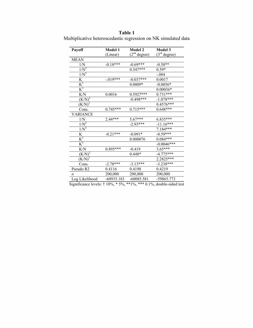
Table 1 Multiplicative heteroscedastic regression on NK simulated data

Payoff Model 1

(Linear) Model 2 (2nd degree)

Model 3 (3rd degree)

MEAN 1/N -0.18*** -0.69*** -0.58** 1/N2 0.547*** 0.59* 1/N3 -.084 K -.019*** -0.037*** 0.0017 K2 0.0009* -0.0056* K3 0.00036* K/N 0.0016 0.5927*** 0.731*** (K/N)2 -0.498*** -1.078*** (K/N)3 0.4576*** Cons. 0.745*** 0.715*** 0.648***

VARIANCE 1/N 2.44*** 5.67*** 6.835*** 1/N2 -2.93*** -11.16*** 1/N3 7.184*** K -0.21*** -0.091* -0.59*** K2 0.000076 0.084*** K3 -0.0046*** K/N 0.895*** -0.419 3.65*** (K/N)2 0.448* -4.775*** (K/N)3 2.2825*** Cons. -2.78*** -3.13*** -3.238***

Pseudo R2 0.4116 0.4198 0.4219 n 200,000 200,000 200,000 Log Likelihood -60935.183 -60085.581 -59865.773

Significance levels: † 10%, * 5%, **1%, *** 0.1%, double-sided test

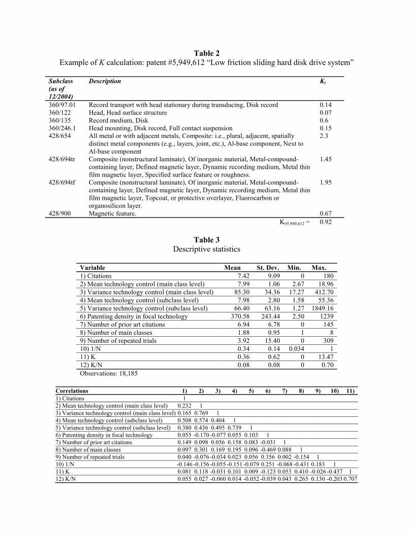
Table 2 Example of K calculation: patent #5,949,612 “Low friction sliding hard disk drive system”

Subclass (as of 12/2004)

Description Ki

360/97.01 Record transport with head stationary during transducing, Disk record 0.14 360/122 Head, Head surface structure 0.07 360/135 Record medium, Disk 0.6 360/246.1 Head mounting, Disk record, Full contact suspension 0.15 428/654 All metal or with adjacent metals, Composite: i.e., plural, adjacent, spatially

distinct metal components (e.g., layers, joint, etc.), Al-base component, Next to Al-base component

2.3

428/694tr Composite (nonstructural laminate), Of inorganic material, Metal-compound-containing layer, Defined magnetic layer, Dynamic recording medium, Metal thin film magnetic layer, Specified surface feature or roughness.

1.45

428/694tf Composite (nonstructural laminate), Of inorganic material, Metal-compound-containing layer, Defined magnetic layer, Dynamic recording medium, Metal thin film magnetic layer, Topcoat, or protective overlayer, Fluorocarbon or organosilicon layer.

1.95

428/900 Magnetic feature. 0.67 K#5,949,612 = 0.92

Table 3 Descriptive statistics

Variable Mean St. Dev. Min. Max. 1) Citations 7.42 9.09 0 180 2) Mean technology control (main class level) 7.99 1.06 2.67 18.96 3) Variance technology control (main class level) 85.30 34.36 17.27 412.70 4) Mean technology control (subclass level) 7.98 2.80 1.58 55.36 5) Variance technology control (subclass level) 66.40 63.16 1.27 1849.16 6) Patenting density in focal technology 370.58 243.44 2.50 1239 7) Number of prior art citations 6.94 6.78 0 145 8) Number of main classes 1.88 0.95 1 8 9) Number of repeated trials 3.92 15.40 0 309 10) 1/N 0.34 0.14 0.034 1 11) K 0.36 0.62 0 13.47 12) K/N 0.08 0.08 0 0.70 Observations: 18,185

Correlations 1) 2) 3) 4) 5) 6) 7) 8) 9) 10) 11) 1) Citations 1 2) Mean technology control (main class level) 0.232 1 3) Variance technology control (main class level) 0.165 0.769 1 4) Mean technology control (subclass level) 0.508 0.574 0.404 1 5) Variance technology control (subclass level) 0.380 0.436 0.495 0.739 1 6) Patenting density in focal technology 0.055 -0.170 -0.077 0.055 0.103 1 7) Number of prior art citations 0.149 0.098 0.056 0.158 0.083 -0.031 1 8) Number of main classes 0.097 0.301 0.169 0.195 0.096 -0.469 0.088 1 9) Number of repeated trials 0.040 -0.076 -0.034 0.023 0.056 0.356 0.002 -0.154 1 10) 1/N -0.146 -0.156 -0.055 -0.151 -0.079 0.251 -0.068 -0.431 0.183 1 11) K 0.081 0.118 -0.031 0.101 0.009 -0.123 0.053 0.410 -0.026 -0.437 1 12) K/N 0.055 0.027 -0.060 0.014 -0.052 -0.039 0.043 0.265 0.130 -0.203 0.707

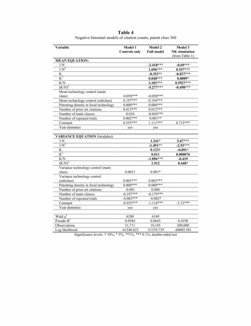
Table 4 Negative binomial models of citation counts, patent class 360

Variable Model 1

Controls only Model 2

Full model Model 3

NK simulation (from Table 1)

MEAN EQUATION: 1/N -2.418*** -0.69*** 1/N2 1.696*** 0.547*** K -0.353** -0.037*** K2 0.048*** 0.0009* K/N 3.183*** 0.5927*** (K/N)2 -5.277*** -0.498*** Mean technology control (main class) -0.058*** -0.050***

Mean technology control (subclass) 0.197*** 0.194*** Patenting density in focal technology 0.000*** 0.000*** Number of prior art citations 0.013*** 0.012*** Number of main classes 0.010 -0.044*** Number of repeated trials 0.002*** 0.001** Constant 0.555*** 1.111*** 0.715*** Year dummies yes yes

VARIANCE EQUATION (ln(alpha))

1/N 1.241* 5.67*** 1/N2 -1.491** -2.93*** K 0.123† -0.091* K2 0.011 0.000076 K/N -1.896*** -0.419 (K/N)2 1.912 0.448* Variance technology control (main class) 0.001† 0.001*

Variance technology control (subclass) 0.003*** 0.003***

Patenting density in focal technology 0.000*** 0.000*** Number of prior art citations -0.001 0.000 Number of main classes -0.197*** -0.179*** Number of repeated trials -0.002*** -0.002* Constant -0.935*** -1.118*** -3.13*** Year dummies yes yes

Wald χ2 6288 6169 Pseudo R2 0.0584 0.0643 0.4198 Observations 21,711 18,185 200,000 Log likelihood -61540.623 -51539.739 -60085.581

Significance levels: † 10%, * 5%, **1%, *** 0.1%, double-sided test

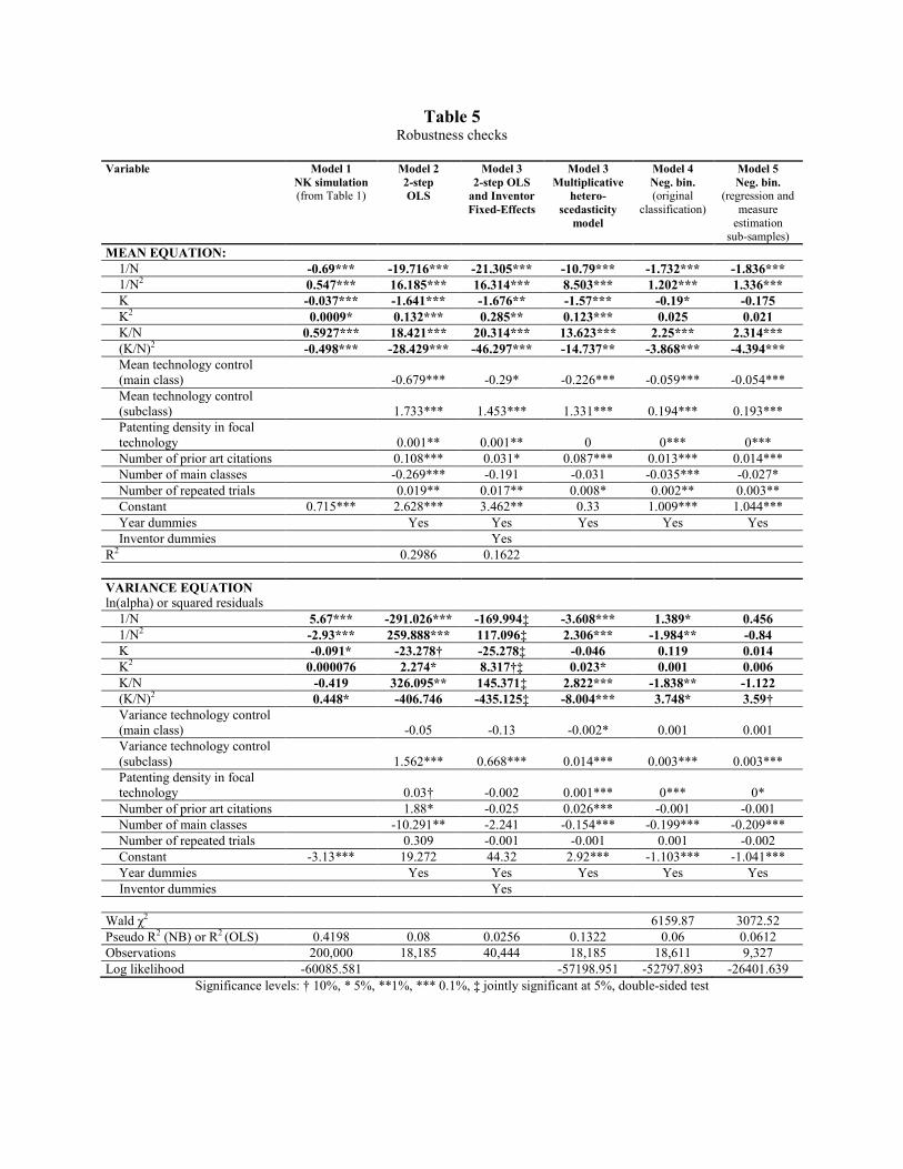
Table 5 Robustness checks

Variable Model 1

NK simulation (from Table 1)

Model 2 2-step OLS

Model 3 2-step OLS and Inventor Fixed-Effects

Model 3 Multiplicative

hetero- scedasticity

model

Model 4 Neg. bin. (original

classification)

Model 5 Neg. bin.

(regression and measure

estimation sub-samples)

MEAN EQUATION: 1/N -0.69*** -19.716*** -21.305*** -10.79*** -1.732*** -1.836*** 1/N2 0.547*** 16.185*** 16.314*** 8.503*** 1.202*** 1.336*** K -0.037*** -1.641*** -1.676** -1.57*** -0.19* -0.175 K2 0.0009* 0.132*** 0.285** 0.123*** 0.025 0.021 K/N 0.5927*** 18.421*** 20.314*** 13.623*** 2.25*** 2.314*** (K/N)2 -0.498*** -28.429*** -46.297*** -14.737** -3.868*** -4.394*** Mean technology control (main class)

-0.679*** -0.29* -0.226*** -0.059*** -0.054***

Mean technology control (subclass)

1.733*** 1.453*** 1.331*** 0.194*** 0.193***

Patenting density in focal technology

0.001** 0.001** 0 0*** 0***

Number of prior art citations 0.108*** 0.031* 0.087*** 0.013*** 0.014*** Number of main classes -0.269*** -0.191 -0.031 -0.035*** -0.027* Number of repeated trials 0.019** 0.017** 0.008* 0.002** 0.003** Constant 0.715*** 2.628*** 3.462** 0.33 1.009*** 1.044*** Year dummies Yes Yes Yes Yes Yes Inventor dummies Yes

R2 0.2986 0.1622 VARIANCE EQUATION ln(alpha) or squared residuals

1/N 5.67*** -291.026*** -169.994‡ -3.608*** 1.389* 0.456 1/N2 -2.93*** 259.888*** 117.096‡ 2.306*** -1.984** -0.84 K -0.091* -23.278† -25.278‡ -0.046 0.119 0.014 K2 0.000076 2.274* 8.317†‡ 0.023* 0.001 0.006 K/N -0.419 326.095** 145.371‡ 2.822*** -1.838** -1.122 (K/N)2 0.448* -406.746 -435.125‡ -8.004*** 3.748* 3.59† Variance technology control (main class)

-0.05 -0.13 -0.002* 0.001 0.001

Variance technology control (subclass)

1.562*** 0.668*** 0.014*** 0.003*** 0.003***

Patenting density in focal technology

0.03† -0.002 0.001*** 0*** 0*

Number of prior art citations 1.88* -0.025 0.026*** -0.001 -0.001 Number of main classes -10.291** -2.241 -0.154*** -0.199*** -0.209*** Number of repeated trials 0.309 -0.001 -0.001 0.001 -0.002 Constant -3.13*** 19.272 44.32 2.92*** -1.103*** -1.041*** Year dummies Yes Yes Yes Yes Yes Inventor dummies Yes

Wald χ2 6159.87 3072.52 Pseudo R2 (NB) or R2 (OLS) 0.4198 0.08 0.0256 0.1322 0.06 0.0612 Observations 200,000 18,185 40,444 18,185 18,611 9,327 Log likelihood -60085.581 -57198.951 -52797.893 -26401.639

Significance levels: † 10%, * 5%, **1%, *** 0.1%, ‡ jointly significant at 5%, double-sided test

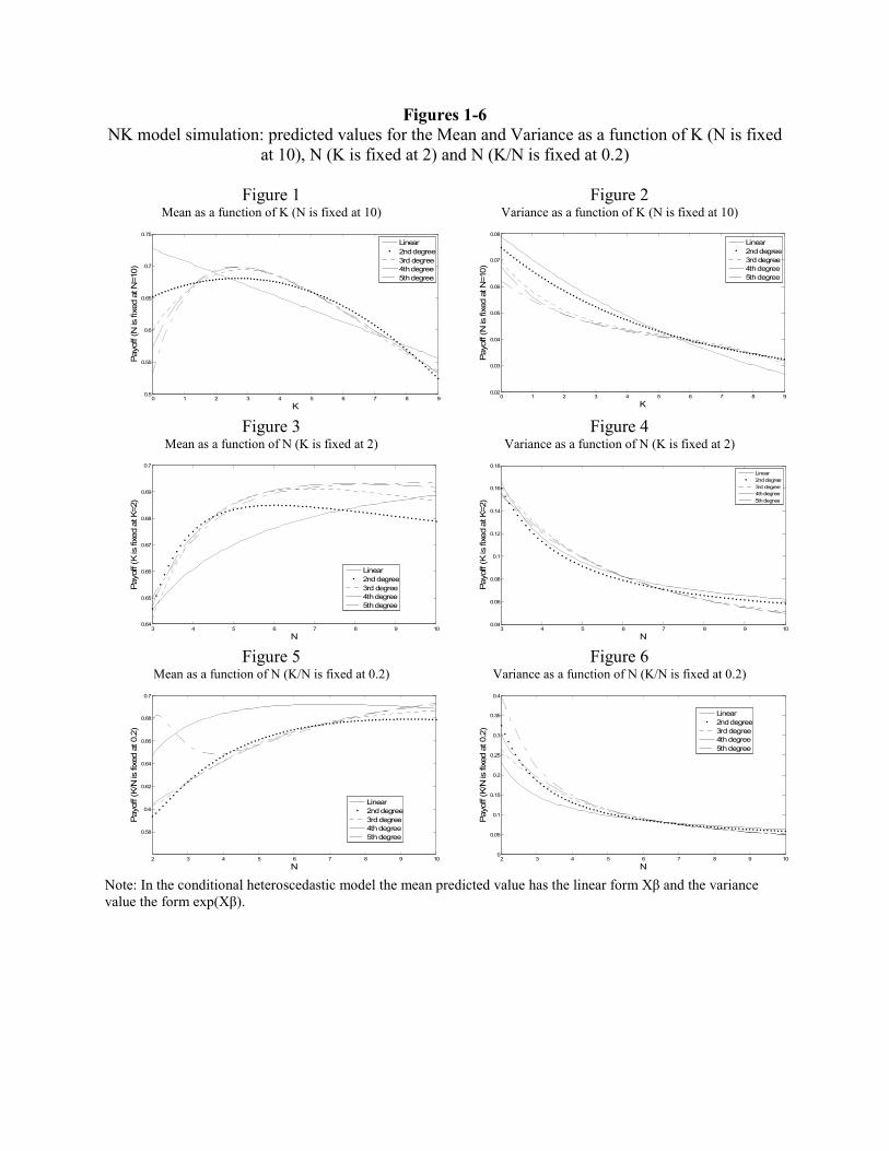
Figures 1-6 NK model simulation: predicted values for the Mean and Variance as a function of K (N is fixed

at 10), N (K is fixed at 2) and N (K/N is fixed at 0.2)

Figure 1 Mean as a function of K (N is fixed at 10)

0 1 2 3 4 5 6 7 8 90.5

0.55

0.6

0.65

0.7

0.75

K

Payoff (N is fixed at N=10)

Linear2nd degree3rd degree4th degree5th degree

Figure 2 Variance as a function of K (N is fixed at 10)

0 1 2 3 4 5 6 7 8 90.02

0.03

0.04

0.05

0.06

0.07

0.08

K

Payoff (N is fixed at N=10)

Linear2nd degree3rd degree4th degree5th degree

Figure 3 Mean as a function of N (K is fixed at 2)

3 4 5 6 7 8 9 100.64

0.65

0.66

0.67

0.68

0.69

0.7

N

Payoff (K is fixed at K=2)

Linear2nd degree3rd degree4th degree5th degree

Figure 4 Variance as a function of N (K is fixed at 2)

3 4 5 6 7 8 9 100.04

0.06

0.08

0.1

0.12

0.14

0.16

0.18

N

Payoff (K is fixed at K=2)

Linear2nd degree3rd degree4th degree5th degree

Figure 5 Mean as a function of N (K/N is fixed at 0.2)

2 3 4 5 6 7 8 9 10

0.58

0.6

0.62

0.64

0.66

0.68

0.7

N

Payoff (K/N is fixed at 0.2)

Linear2nd degree3rd degree4th degree5th degree

Figure 6 Variance as a function of N (K/N is fixed at 0.2)

2 3 4 5 6 7 8 9 100

0.05

0.1

0.15

0.2

0.25

0.3

0.35

0.4

N

Payoff (K/N is fixed at 0.2)

Linear2nd degree3rd degree4th degree5th degree

Note: In the conditional heteroscedastic model the mean predicted value has the linear form Xβ and the variance value the form exp(Xβ).

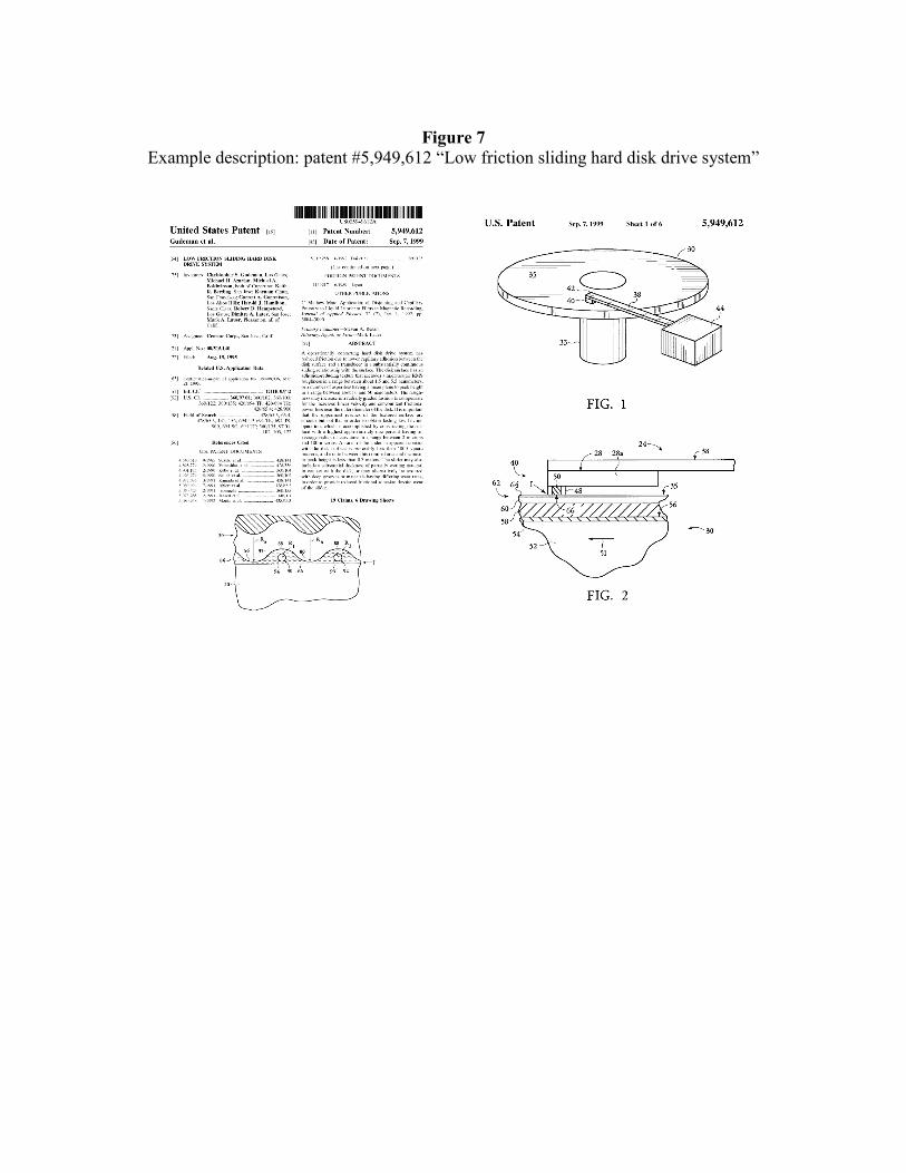
Figure 7

Example description: patent #5,949,612 “Low friction sliding hard disk drive system”

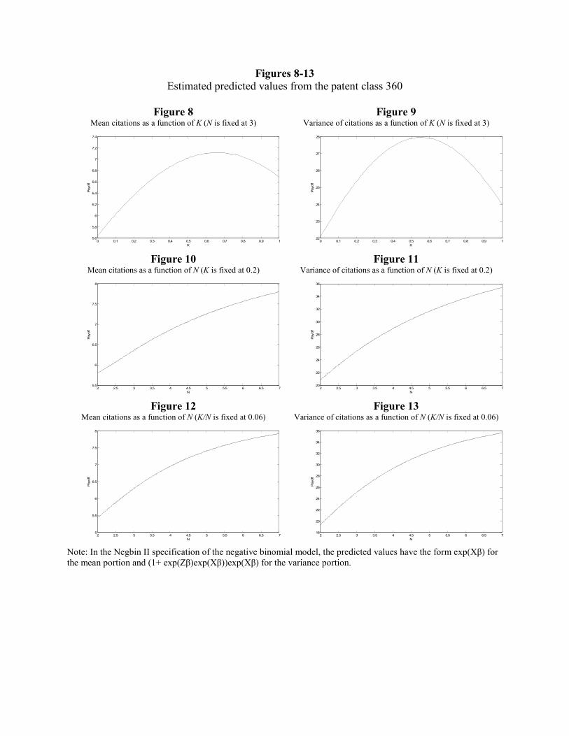
Figures 8-13 Estimated predicted values from the patent class 360

Figure 8

Mean citations as a function of K (N is fixed at 3)

0 0.1 0.2 0.3 0.4 0.5 0.6 0.7 0.8 0.9 15.6

5.8

6

6.2

6.4

6.6

6.8

7

7.2

7.4

K

Payoff

Figure 9 Variance of citations as a function of K (N is fixed at 3)

0 0.1 0.2 0.3 0.4 0.5 0.6 0.7 0.8 0.9 122

23

24

25

26

27

28

K

Payoff

Figure 10 Mean citations as a function of N (K is fixed at 0.2)

2 2.5 3 3.5 4 4.5 5 5.5 6 6.5 75.5

6

6.5

7

7.5

8

N

Payoff

Figure 11 Variance of citations as a function of N (K is fixed at 0.2)

2 2.5 3 3.5 4 4.5 5 5.5 6 6.5 720

22

24

26

28

30

32

34

36

N

Payoff

Figure 12 Mean citations as a function of N (K/N is fixed at 0.06)

2 2.5 3 3.5 4 4.5 5 5.5 6 6.5 75

5.5

6

6.5

7

7.5

8

N

Payoff

Figure 13 Variance of citations as a function of N (K/N is fixed at 0.06)

2 2.5 3 3.5 4 4.5 5 5.5 6 6.5 718

20

22

24

26

28

30

32

34

36

N

Payoff

Note: In the Negbin II specification of the negative binomial model, the predicted values have the form exp(Xβ) for the mean portion and (1+ exp(Zβ)exp(Xβ))exp(Xβ) for the variance portion.

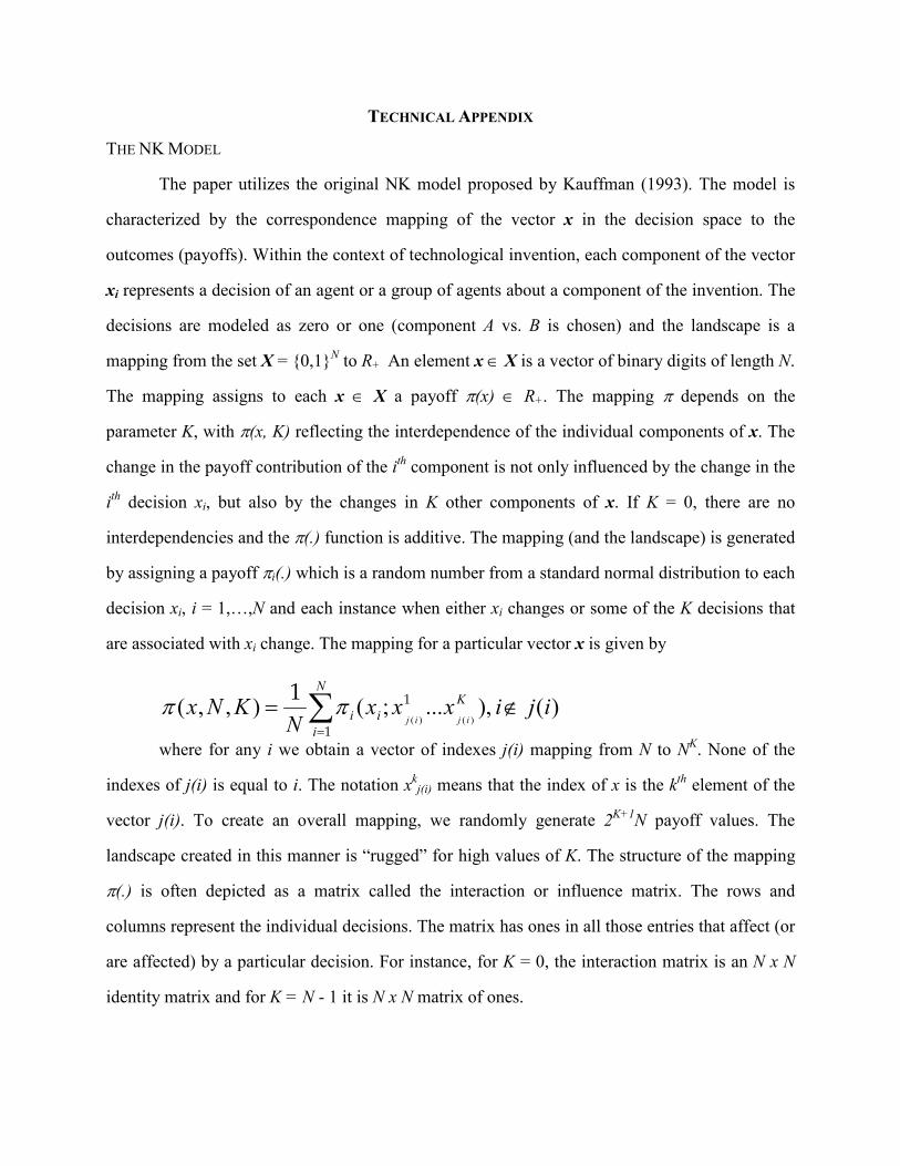
TECHNICAL APPENDIX

THE NK MODEL

The paper utilizes the original NK model proposed by Kauffman (1993). The model is

characterized by the correspondence mapping of the vector x in the decision space to the

outcomes (payoffs). Within the context of technological invention, each component of the vector

xi represents a decision of an agent or a group of agents about a component of the invention. The

decisions are modeled as zero or one (component A vs. B is chosen) and the landscape is a

mapping from the set X = {0,1}N to R+ An element x ∈ X is a vector of binary digits of length N.

The mapping assigns to each x ∈ X a payoff π(x) ∈ R+. The mapping π depends on the

parameter K, with π(x, K) reflecting the interdependence of the individual components of x. The

change in the payoff contribution of the ith component is not only influenced by the change in the

ith decision xi, but also by the changes in K other components of x. If K = 0, there are no

interdependencies and the π(.) function is additive. The mapping (and the landscape) is generated

by assigning a payoff πi(.) which is a random number from a standard normal distribution to each

decision xi, i = 1,…,N and each instance when either xi changes or some of the K decisions that

are associated with xi change. The mapping for a particular vector x is given by

where for any i we obtain a vector of indexes j(i) mapping from N to NK. None of the

indexes of j(i) is equal to i. The notation xkj(i) means that the index of x is the kth element of the

vector j(i). To create an overall mapping, we randomly generate 2K+1N payoff values. The

landscape created in this manner is “rugged” for high values of K. The structure of the mapping

π(.) is often depicted as a matrix called the interaction or influence matrix. The rows and

columns represent the individual decisions. The matrix has ones in all those entries that affect (or

are affected) by a particular decision. For instance, for K = 0, the interaction matrix is an N x N

identity matrix and for K = N - 1 it is N x N matrix of ones.

)( ),...;(),,()()(

ijixxxN

KNx Ki

N

ii ijij

∉= ∑=

1

1

1ππ

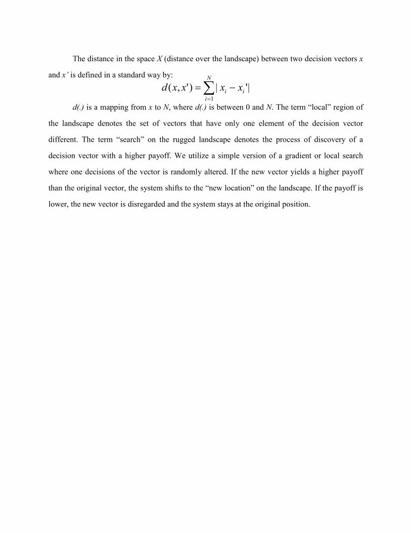
The distance in the space X (distance over the landscape) between two decision vectors x

and x’ is defined in a standard way by:

∑=

−=N

iii xxxxd

1

|'|)',(

d(.) is a mapping from x to N, where d(.) is between 0 and N. The term “local” region of

the landscape denotes the set of vectors that have only one element of the decision vector

different. The term “search” on the rugged landscape denotes the process of discovery of a

decision vector with a higher payoff. We utilize a simple version of a gradient or local search

where one decisions of the vector is randomly altered. If the new vector yields a higher payoff

than the original vector, the system shifts to the “new location” on the landscape. If the payoff is

lower, the new vector is disregarded and the system stays at the original position.