Invasion fronts on graphs: the Fisher-KPP equation on

homogeneous trees and Erdos-Reyni graphs

Aaron Hoffman1 and Matt Holzer∗2

1Franklin W. Olin College of Engineering, Needham, MA 02492, USA2George Mason University, Department of Mathematical Sciences, Fairfax, VA 22030, USA

May 4, 2018

Abstract

We study the dynamics of the Fisher-KPP equation on the infinite homogeneous tree and

Erdos-Reyni random graphs. We assume initial data that is zero everywhere except at a single

node. For the case of the homogeneous tree, the solution will either form a traveling front or

converge pointwise to zero. This dichotomy is determined by the linear spreading speed and

we compute critical values of the diffusion parameter for which the spreading speed is zero and

maximal and prove that the system is linearly determined. We also study the growth of the

total population in the network and identify the exponential growth rate as a function of the

diffusion coefficient, α. Finally, we make predictions for the Fisher-KPP equation on Erdos-

Renyi random graphs based upon the results on the homogeneous tree. When α is small we

observe via numerical simulations that mean arrival times are linearly related to distance from

the initial node and the speed of invasion is well approximated by the linear spreading speed

on the tree. Furthermore, we observe that exponential growth rates of the total population on

the random network can be bounded by growth rates on the homogeneous tree and provide an

explanation for the sub-linear exponential growth rates that occur for small diffusion.

Keywords: invasion fronts, linear spreading speed, homogeneous tree, random graph

1 Introduction

We consider the Fisher-KPP equation defined on a graph and study the transition of the system

from unstable to stable homogeneous states. To provide some motivation for this study we consider

the dynamics of an invasive species on a transportation network. One can think of each node in

the network as describing a physical location and the edges connecting these nodes as available

∗mholzer@gmu.edu, 703-993-1460

1

arX

iv:1

610.

0687

7v3

[nl

in.P

S] 2

May

201

8

transportation routes between these locales. When the invasive species is introduced at one location

in the network we expect the species to grow and spread through the network until it resides at

every node in the network that is favorable to the species. The goal would be to determine in what

manner this transition occurs and to estimate the time that is required for the species to arrive at

any given node in the network.

A realistic description of this process would involve complicated network topologies and a great

deal of heterogeneity – both in the local dynamics of the species at each node as well as the

transportation mechanisms available to move between modes. Our focus in this paper is to study a

simplified version of this problem where the local dynamics are identical and prescribed by logistic

growth while the movement between nodes is encapsulated by diffusion. In regards to network

topologies, we concentrate mainly on the case where the network is a homogeneous tree. This

restriction allows us to make precise statements regarding the dynamics of the system, which

then serve as a baseline for comparison with numerical studies of more complicated and realistic

situations.

To be precise, let G = (V,E) be a undirected and unweighted countable graph; we will mainly

be interested in the infinite homogeneous tree, but leave the discussion general for the time being

leave. Consider a differential equation defined on the set of vertices with local dynamics prescribed

by the scalar differential equation ut = f(u). The reaction term f(u) ∈ C1([0, 1]) is assumed to be

of KPP type, see [16, 20], and satisfies the conditions,

f(0) = f(1) = 0

f ′(0) > 0, f ′(1) < 0

f(u) > 0 for 0 < u < 1

f(u) < f ′(0)u for 0 < u < 1.

We can assume further that f ′(0) = 1 after rescaling the independent variable. In most of the

numerical simulations contained in this paper we use the explicit example of logistic growth, f(u) =

u(1 − u). Diffusion between nodes is incorporated by the graph Laplacian, ∆G = A(G) − D(G)

where A(G) is the adjacency matrix and D(G) is diagonal with ith entry equal to the degree of

the ith node. Incorporating both the local dynamics and diffusion between nodes we arrive at the

reaction-diffusion equation that will be the main focus of this article,

ut = α∆Gu+ f(u). (1.1)

The dependent variable ui ∈ R can be thought of as representing the population of a species residing

at node i ∈ V .

Consider initial conditions where the population of the species is zero everywhere in the graph

aside from one node where some positive concentration exists. Due to diffusion, the population will

spread out into the graph.

We are interested in both the pointwise and aggregate behavior of the population. For the

infinite tree, we will be particularly interested in the existence/ non-existence of traveling fronts

2

that propagate asymptotically with fixed speed and replace the unstable state at zero with the

stable steady state at one. When these fronts exist, their speeds provide a measure of how long it

takes for the invasive species to overtake a node as a function of the distance of that node from

the node of introduction. For sufficiently large values of the diffusion parameter α, we find that

compactly supported initial data converges pointwise to zero. It is important to note that this is

not representative of the extinction of the species. In studying the aggregate behavior we focus on

the dynamics of the total population; that is the sum of the population over all the nodes in the

graph. We find that this growth rate is always positive. Of particular interest is how this growth

rate depends on system parameters and its relation to the existence/ non-existence of traveling

fronts.

The situation is somewhat different for finite connected Erdos-Reyni graphs since the steady state

at one is a global attractor of the dynamics. Here we study arrival times describing how long

it takes the species to reach any given node. We are interested in whether the arrival times are

approximately linear with respect to the distances from the node of origination. When α is small

we observe this to be the case numerically and we draw analogies between this behavior and the

propagation of traveling fronts.

Let us now focus on the case where G is an infinite homogeneous tree where each node has degree

k + 1. Identify one node as the root, label it u1, and consider initial conditions wherein u1(0) = 1

with all other nodes initially equal to zero. For this initial data, (1.1) can be reduced to the lattice

dynamical system,

dundt

= α (un−1 − (k + 1)un + kun+1) + f(un), n ≥ 2,

du1

dt= α(k + 1) (−u1 + u2) + f(u1). (1.2)

where un(t) is a representative node from the set of nodes at distance n− 1 from the root.

The evolution equation for any non-root node of the tree can be expressed as

dundt

= α (un−1 − 2un + un+1) + α(k − 1) (un+1 − un) + f(un). (1.3)

In this way, the linear terms in (1.2) can be viewed as a competition between diffusive and advective

effects. Take α = 1(∆x)2

for some small ∆x. Then the first term on the right hand side of (1.3) can

be viewed as a discretization of the second derivative while the second term can be viewed as a

discretization of the first derivative. Therefore, in the continuum limit the dynamics are formally

approximated by the solution of PDE,

ut = uxx +√α(k − 1)ux + f(u),

on a semi-infinite domain with no-flux boundary conditions at the left boundary. In this scenario,

the advection dominates the diffusion and localized initial data propagates to the left, i.e. up the

tree, and eventually converges to zero. On the other hand, when α is small and the system is near

the anti-continuum limit, the reaction terms dominate the diffusive ones and localized initial data

3

will spread down the tree. The goal of this article is to understand the transition from spreading

to pointwise convergence to zero and, in the case of spreading, to predict the spreading speed of

the solution to (1.2).

There has been a tremendous amount of effort dedicated to the study of the Fisher-KPP equation

in a variety of contexts. The system was initially studied as a PDE on the real line by Fisher [16]

and Kolmogorov, Petrovskii and Piscunov [20]. In the context of lattice dynamical systems, the

existence of traveling waves was established in [32]. Most related to the current study is recent

work in [22] where spreading speeds for the Fisher-KPP equation on the hyperbolic space Hn are

investigated. Homogeneous trees are often used as a model for Hn and there are strong connections

between the results obtained here and those in [22]. Indeed, in [22] it is shown that there exists a

critical diffusion coefficient above which the solution converges uniformly to zero, while for values

below that threshold compactly supported initial data form a traveling front.

The previous two decades has also witnessed an explosion of interest into the dynamics of differential

equations on networks; see [24, 25, 27, 29] and the references therein for an overview of the field.

Many studies of dynamical systems on networks treat each node as an individual with discrete

state. The present work deals with meta-population models, where the dependent variable at each

node describes the concentration of individuals; see for example [8, 13, 17] for studies of disease

epidemics within the meta-population paradigm. The work undertaken here is related to [9]. There

the Fisher-KPP equation on random graphs is studied with a focus on the growth rate of the overall

population in the network. Exponential growth rates of the population are studied and sub-linear

growth rates are observed for small values of the diffusion parameter. Finally, we also mention [21]

where a bistable reaction-diffusion equation is considered and the existence of traveling and pinned,

or stationary, fronts are exhibited on random networks and trees.

We now outline our main results, beginning with those that pertain to the case of the infinite

homogeneous tree.

Linearly selected spreading speeds – l1 and l2 critical diffusion coefficients A key feature

of the dynamics of (1.2) is non-monotonicity of the spreading speed. We identify two critical

diffusion coefficients: α1(k) and α2(k). The spreading speed is maximal for α1(k) while for α2(k)

the spreading speed is zero and marks the boundary between spreading and non-spreading. For

any 0 < α < α2(k), the initial value problem (1.2) forms a traveling front spreading with the linear

spreading speed. For α > α2(k) the solution converges pointwise exponentially fast to zero. The

decay rate of the selected front is l1 critical at α1 and l2 critical for α2.

We also consider the generalization of (1.2) to periodic trees, where the number of children at each

level is periodic. In this case a similar reduction to a lattice dynamical system is possible. In

analogy with the homogeneous case, we observe that the linear spreading speed for this system is

zero when the selected decay rate is l2 critical and the spreading speed has a critical point when

the selected decay rate is l1 critical.

It is interesting to contrast these dynamics with the case of the classical Fisher-KPP equation on

4

the real line. In that case, as the diffusion parameter α is increased the solution propagates with

an increased speed. This makes intuitive sense, as increasing the diffusion constant corresponds to

increasing the mobility of the species being modeled. On the infinite tree, it would appear that for

α > α1(k), increasing the mobility of the species decreases the speed at which it invades. However,

we emphasize that while the solution to (1.2) slows down with increasing α > α1, the invasion of

the species does not.

When α is small the reactive effects dominate the diffusive ones and we obtain an asymptotic

expansion of the spreading speed as α(k)→ 0. This expansion is independent of k to leading order.

We therefore predict that dynamics of (1.2) on more general networks should also be independent

of the network topology for α sufficiently small. We test this prediction on Erdos-Renyi random

graphs.

Growth rate of the total population We also study the total population on the graph – both

in aggregate and at each level of the tree. Our main contribution here is to identify the maximal

growth rate of the total population and to locate which levels of the tree this maximal population

growth is concentrated on as a function of time.

The exponential growth rate of the population in the linear system is one. In the nonlinear system,

growth is saturated at u = 1 and we expect that the growth rate of the population may be slower

in this case. In turns out that the critical diffusion parameter α1(k) demarcates the boundary

between these two possibilities. For α < α1(k), the population growth occurs primarily at the front

interface and the maximal growth rate depends on the speed and decay rate of the front. When

α is larger than α1(k), the maximal growth rate is one and occurs in a region ahead of the front

interface where the components un(t) are near zero. The speed at which the maximal growth rate

occurs can be determined in terms of the group velocity of the mode kn.

Front propagation and population growth rates on Erdos-Renyi random graphs: nu-

merical simulations Finally, we address the potential relevance of our results to large, but finite,

random graphs of Erdos-Renyi type, [15]. When the number of nodes in the network is large and

the average degree of each node is small it may be reasonable to approximate the dynamics on the

random graph by that of a tree with k chosen appropriately. We perform numerical simulations

that suggest that for small values of α, the dynamics of (1.1) are well approximated by the finite

homogeneous tree. We also consider the growth rate of the total population on the graph and

demonstrate that this rate can be estimated from the growth rate on the homogeneous tree. In

analogy to the tree case, for small values of α the growth rate is observed to be less than the linear

growth rate.

The article is organized as follows. In Section 2, we study the pointwise behavior of the solution

on the homogeneous tree and prove Theorem 1. In Section 3, we study the behavior of the total

population in the tree. In Section 4, we apply some of the insights gained from the homogeneous

tree to Erdos-Renyi random graphs. We conclude in Section 5 with a short discussion.

5

2 Front propagation – the linear spreading speed and proof of

Theorem 1

In this section, we study the dynamics of (1.2) and establish the spreading speed (or lack thereof) of

solutions propagating down the tree. We first review the notion of linear spreading speeds. We then

establish some properties of the linear spreading speed for (1.2) and identify the critical coefficients

α1(k) and α2(k). Noteworthy among these properties is the independence of the spreading speed

on the constant k in the asymptotic limit of α small. Finally, we establish that the linear spreading

speed is the speed selected in the nonlinear system and we extend the linear spreading speed to the

case of periodic trees.

The Fisher-KPP equation, whether it be posed on the real line, lattice or other more exotic domain

is an example of a linearly determinate system wherein the spreading speed for the full nonlinear

system is equal to the spreading speed of the system linearized about the unstable state; see for

example [31]. In this regard, a natural starting point for our analysis is system (1.2) linearized

about the unstable zero state. Ignoring the equation for the root, we obtain the linearized problem,

dundt

= α (un−1 − (k + 1)un + kun+1) + un, n ≥ 2. (2.1)

We seek separable solutions of the form eλt−γn, γ > 0, and obtain a solvability condition that is

known as the dispersion relation,

d(λ, γ) = α(eγ − k − 1 + ke−γ

)+ 1− λ. (2.2)

Simple roots of the dispersion relation relate exponentially decaying modes e−γn to their temporal

growth rate eλt. Double roots, or more precisely pinched double roots, of (2.2) identify pointwise

growth rates of compactly supported initial data; see for example [3, 6, 7, 19, 26, 28]. Double roots

differentiate between absolute and convective instabilities. In the context of (2.1), an absolute

instablity refers to exponential growth of both the solution in norm (l2 for example) as well as

pointwise at each fixed node. On the other hand, a convective instablity grows in norm, but is

transported away from its original location so that the solution decays pointwise at each node. A

convective instability is one where the dispersion relation has simple roots with positive temporal

growth rates, but all pinched double roots have negative growth rates, i.e. Re(λ) < 0.

The linear spreading speed is the speed at which compactly supported initial data spreads in

the asymptotic limit as t → ∞. This speed can be thought of as the speed for which the system

transitions from absolute to convective instability and is defined by the presense of a pinched double

root with purely imaginary, or in our case zero, temporal growth rate. We therefore consider the

dispersion relation (2.2) in a co-moving frame. Let ds(λ, γ) = d(λ − sγ, γ) denote the dispersion

relation in this frame. Then the linear spreading speed for (2.2) is the speed slin for which a γlin

simultaneously satisfies the equations,

dslin(0, γlin) = 0, ∂γdslin(0, γlin) = 0,

6

together with a pinching condition. Pinching here refers to the requirement that the roots partici-

pating in the double root can be traced to opposite sides of the imaginary axis as Re(λ)→∞.

In order to introduce some further terminology we also mention an alternate, and equivalent,

formulation of the linear spreading speed as a minimizer of the envelope velocity,

senv(γ) = α

(eγ − k − 1 + ke−γ

γ

)+

1

γ.

The envelope velocity prescribes the speed at which an exponential solution e−γn propagates in

the linear equation (2.1). For systems that obey the comparison principle, any positive solution of

the linearized system places an upper bound on the speed of propagation in the nonlinear system

and so minimizing over all such speeds provides an upper bound. In this way, the linear spreading

speed can be alternatively defined as

slin = minγ∈R+

senv(γ).

The equivalence of these two formulations can be observed by imposing that

0 = ∂γsenv(γ) =1

γ

(dλ

dγ− senv

).

The quantity dλdγ is known as the group velocity and so the linear spreading speed occurs when the

group velocity equals the envelope velocity. In a frame moving at the envelope velocity, this then

implies zero group velocity and hence that γ is a pinched double root with s = senv. The notion of

group velocity will arise again in Section 3.

Moving forward, we will use the formulation in terms of pinched double roots and define

F (s, γ, α) =

(α (eγ − k − 1 + ke−γ)− sγ + 1

α (eγ − ke−γ)− s

). (2.3)

2.1 Properties of the linear spreading speed for (2.1)

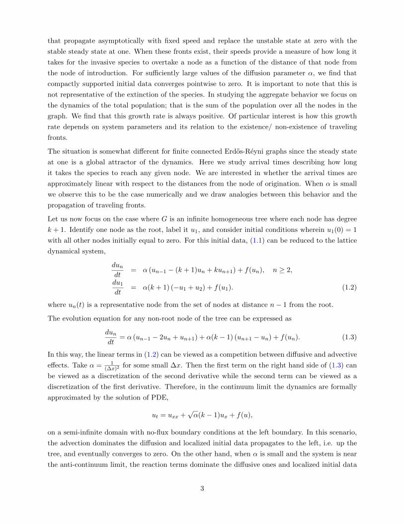
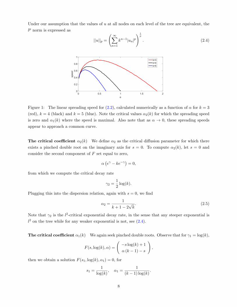
Inspection of (2.3) reveals that explicit expressions for the linear spreading speed are not available.

We compute solutions numerically and plot the linear spreading speed in Figure 1. Two features of

the linear spreading speed are readily apparent: it is non-monotone as a function of α and becomes

negative above some critical value. In what follows, we identify the linear spreading speed at two

critical values of the diffusion parameter: the diffusion coefficient leading to the fastest spreading

speed we denote α1(k) whereas the diffusion coefficient with zero spreading speed we denote α2(k).

The notation is chosen since we will show that for α1 and α2 the decay rates of the fronts are

critical in l1 and l2 respectively. Recall the definition of the lp norm on G,

||u||p =

(∑v∈V|uv|p

) 1p

.

7

Under our assumption that the values of u at all nodes on each level of the tree are equivalent, the

lp norm is expressed as

||u||p =

( ∞∑n=1

kn−1|un|p) 1

p

. (2.4)

0 0.5 1 1.5 2

α

0

0.2

0.4

0.6

0.8

1

speed

k=3k=4k=5

Figure 1: The linear spreading speed for (2.2), calculated numerically as a function of α for k = 3

(red), k = 4 (black) and k = 5 (blue). Note the critical values α2(k) for which the spreading speed

is zero and α1(k) where the speed is maximal. Also note that as α → 0, these spreading speeds

appear to approach a common curve.

The critical coefficient α2(k) We define α2 as the critical diffusion parameter for which there

exists a pinched double root on the imaginary axis for s = 0. To compute α2(k), let s = 0 and

consider the second component of F set equal to zero,

α(eγ − ke−γ

)= 0,

from which we compute the critical decay rate

γ2 =1

2log(k).

Plugging this into the dispersion relation, again with s = 0, we find

α2 =1

k + 1− 2√k. (2.5)

Note that γ2 is the l2-critical exponential decay rate, in the sense that any steeper exponential is

l2 on the tree while for any weaker exponential is not, see (2.4).

The critical coefficient α1(k) We again seek pinched double roots. Observe that for γ1 = log(k),

F (s, log(k), α) =

(−s log(k) + 1

α (k − 1)− s

),

then we obtain a solution F (s1, log(k), α1) = 0, for

s1 =1

log(k), α1 =

1

(k − 1) log(k).

8

Compute the Jacobians

Ds,γF (s1, log(k), α1) =

(− log(k) 0

−1 α1(k + 1)

), DαF (s1, log(k), α1) =

(0

k − 1

),

from which the Implicit Function Theorem implies that double roots can be continued as functions

s(α) and γ(α) with

s′ (α1) = 0.

Note that γ1 is the l1-critical decay rate, recall (2.4).

Lemma 2.1. The linear spreading speed is monotone increasing for α < α1(k) and is monotone

decreasing for α1(k) < α < α2(k).

Proof. Solving the second equation in F = 0 for s and plugging into the first equation we obtain

an implicit equation for γ and α given by

α((γ − 1)eγ + (k + 1)− k(γ + 1)e−γ

)= 1.

Fix k and define

G(γ) = (γ − 1)eγ + (k + 1)− k(γ + 1)e−γ .

Note that G(0) = 0, limγ→∞G(γ) =∞ and that G′(γ) > 0. Therefore G is monotone and invertible

on its range. Consequently, for every γ > 0 there exists a α for which F (α(eγ − ke−γ), γ, α) = 0.

We observe that the selected decay rate γ is a decreasing function of α and that the spreading

speed α(eγ − ke−γ) may be negative.

Applying the Implicit Function Theorem we find an expression for

dslindα

=1

γα

(eγ − k − 1 + ke−γ

).

We observe that this zero exactly for α = α1. Differentiating the expression in the parenthesis we

obtain

eγ − ke−γ .

This derivative changes sign exactly at α = α2 and thus eγ − k − 1 + ke−γ is monotone decreasing

for α < α2 and the result follows.

Asymptotics for small α Consider 0 < α � 1. We will derive a the leading order term in an

asymptotic expansion for the linear spreading speed in this limit. Consider the implicit equation

αG(γ) = 1.

In the limit as α tends to zero, it must be the case that G(γ)→∞. Since γ > 0, G(γ) is dominated

by the term γeγ and we expect

γeγ ≈ 1

α.

9

Inverting, the selected decay rate is to leading order

γ = W

(1

α

),

where W is the Lambert W-function. Note that s = αeγ to leading order and obtain

s =1

W(

1α

) ,to leading order. We remark that the linear spreading speed is independent of the degree k to

leading order when α� 1. This means that for α small the spreading speed of the system is close

to the spreading speed of the Fisher-KPP equation on a lattice in the anti-continuum limit and the

arrival time to any node in the tree is dominated by its distance from the root. This has important

implications for applications to more general networks, which we will return to later.

Linear Determinacy We have thus far focused entirely on the spreading properties of the lin-

earized system. We now turn our attention to the nonlinear system and introduce some standard

terminology. Define the invasion point for (1.2) as

κ(t) = supn∈N

{n | un(t) >

1

2

}.

The selected spreading speed is then defined as

ssel = limt→∞

κ(t)

t.

We prove the following theorem which establishes that the selected spreading speed is the linear

spreading speed.

Theorem 1. Consider (1.2) with initial condition u1(0) = 1 and uj(0) = 0 for all j 6= 1. Suppose

that 0 < α < α2(k). Then the selected spreading speed equals the linear spreading speed, i.e.

ssel = slin. For α > α2(k), we have that un(t)→ 0 uniformly as t→∞.

Theorem 1 states that the system is linearly determinate and that the spreading speed of the

nonlinear system is the same as the system linearized about the unstable state. We remark that

had (1.2) been posed on Z, rather than N, then this result would be a direct consequence of [31].

Rather than adapt that proof to this context, we will construct explicit sub and super solutions

that bound the spreading speed of system (1.2). Since the proof proceeds along familiar lines, we

delay its presentation until Appendix A.

2.2 The periodic tree

We now consider the generalization to an infinite rooted tree where the number of nodes per level is

periodic. We again assume initial data consisting of one at the root and zero elsewhere and obtain

10

a similar reduction to a lattice dynamical system with the evolution given by

dundt

= α (un−1 − (kn + 1)un + knun+1) + f(un), n ≥ 2,

du1

dt= α(k1 + 1) (−u1 + u2) + f(u1). (2.6)

where kn is periodic in n with periodic m, i.e. kn+m = kn. Our main goal is to study the linear

spreading speed as a function of α and to show that the l2 critical front is stationary while the l1

front is a critical point of the linear spreading speed.

To this end, we linearize (2.6) about the unstable state at zero and obtain the following equation

at any (non-root) node

dundt

= α (un−1 − (kn + 1)un + knun+1) + un.

We seek separable solutions of the form

un(t) = e−γ(n−st)Un, (2.7)

where γ > 0 and Un is periodic with period m. Since Un is periodic we focus on one segment of

length m which we denote U = (U1, U2, . . . , Um)T . Plugging in the ansatz (2.7), U must satisfy

γsU = αMU + U,

where for m ≥ 3,

Mij(γ) =

eγ j = i− 1 mod m

−(ki + 1) j = i

kie−γ j = i+ 1 mod m

0 else

.

Note that M , after adding an appropriate multiple of the identity is positive, so it has a real

principle eigenvalue λ(γ, p) and corresponding principle eigenvector with positive entries, which we

denote U . In this manner, we obtain a scalar dispersion relation that relates the decay rate γ to

the envelope speed s,

d(γ, s) = αλ(γ)− sγ + 1 = 0.

Pinched double roots are therefore solutions of the system of equations

F (s, γ, α) =

(αλ(γ)− sγ + 1

α∂γλ(γ)− s

). (2.8)

We are interested in the linear spreading speeds corresponding to lp critical decay rates. Critical

fronts in lp have decay rate

γp =

∑mi=1 log(ki)

mp.

Then αp and sp can be defined through the relationship F (sp, γp, αp) = 0 and we may express F

entirely as a function of p. Set the second component of F equal to zero, from which

sp = −αpmp2λ′(p)∑mi=1 log(ki)

.

11

Then for the first component of F to be zero it is required that

αp =−1

λ(p) + λ′(p)p.

Combining these two expressions we obtain an equation for the linear spreading speed as a function

of p, in terms of the principle eigenvalue of M ,

sp =m∑m

i=1 log(ki)

p2λ′(p)

λ(p) + λ′(p)p.

We now express the matrix M in terms of p. We first note that

Mij(γp) =

K

1p j = i− 1 mod m

−(ki + 1) j = i

kiK− 1p j = i+ 1 mod m

0 else

,

where K = (Πmi=1ki)

1m . Before stating our results, we show that M(γp) is similar to M(γq), where

q is the Holder dual of p. To do this, we compute the determinant,

det(M(γ)) = (−1)m+1(k1 . . . kme

−mγ + emγ)

+ ∆(k1, . . . , km),

where the terms ∆(k1, . . . , km) do not depend on γ. With γ = γp, we find

det(M(γp)) = (−1)m+1(

(k1 . . . km)1− 1

p + (k1 . . . km)1p

)+ ∆(k1, . . . , km).

Consequently, the characteristic polynomial is invariant when p is replaced with its Holder dual q

and therefore the matrices M(γp) and M(γq) are similar.

Proposition 2.2. s2 = 0.

Proof. Let q be the Holder dual of p. Making use of the fact that M(p) and M(q) are similar it

follows that λ(p) = λ(q) and hence that λ′(p) = λ′(q)q′. Since q′ = −(q/p)2 this rewrites as

p2λ′(p) + q2λ′(q) = 0

In the case p = q = 2 this reduces to λ′(2) = 0. Thus s2 = 0 as desired.

Proposition 2.3. s1 = m∑log ki

. Further s′1 = 0.

Proof. First, we compute

s′p =m∑m−1

i=1 log(ki)

pλ(2λ′ + pλ′′)

(pλ′ + λ)2

In the case p =∞ (1) the matrix M has row (column) sum zero, hence the vector of all ones is in

its (left) null space. As this vector is positive, it is necessarily the principal (left) eigenvector, hence

zero is the principal eigenvalue. With λ = 0 the expression for sp reduces to mp 1∑log kl

. Further s′pvanishes when λ = 0.

12

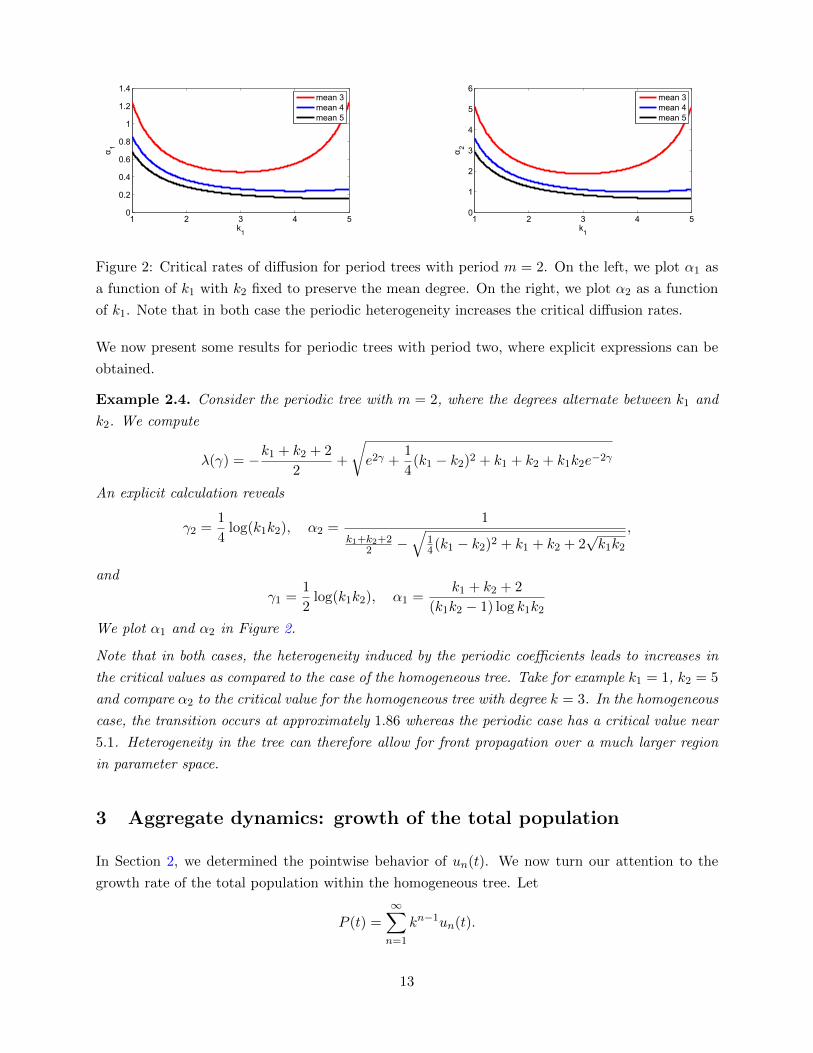
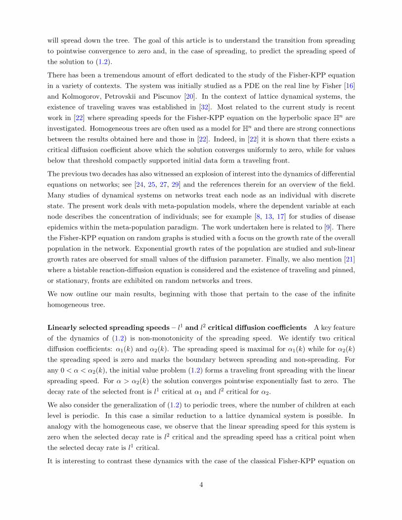
1 2 3 4 50

0.2

0.4

0.6

0.8

1

1.2

1.4

k1

α1

mean 3mean 4mean 5

1 2 3 4 50

1

2

3

4

5

6

k1

α2

mean 3mean 4mean 5

Figure 2: Critical rates of diffusion for period trees with period m = 2. On the left, we plot α1 as

a function of k1 with k2 fixed to preserve the mean degree. On the right, we plot α2 as a function

of k1. Note that in both case the periodic heterogeneity increases the critical diffusion rates.

We now present some results for periodic trees with period two, where explicit expressions can be

obtained.

Example 2.4. Consider the periodic tree with m = 2, where the degrees alternate between k1 and

k2. We compute

λ(γ) = −k1 + k2 + 2

2+

√e2γ +

1

4(k1 − k2)2 + k1 + k2 + k1k2e−2γ

An explicit calculation reveals

γ2 =1

4log(k1k2), α2 =

1

k1+k2+22 −

√14(k1 − k2)2 + k1 + k2 + 2

√k1k2

,

and

γ1 =1

2log(k1k2), α1 =

k1 + k2 + 2

(k1k2 − 1) log k1k2

We plot α1 and α2 in Figure 2.

Note that in both cases, the heterogeneity induced by the periodic coefficients leads to increases in

the critical values as compared to the case of the homogeneous tree. Take for example k1 = 1, k2 = 5

and compare α2 to the critical value for the homogeneous tree with degree k = 3. In the homogeneous

case, the transition occurs at approximately 1.86 whereas the periodic case has a critical value near

5.1. Heterogeneity in the tree can therefore allow for front propagation over a much larger region

in parameter space.

3 Aggregate dynamics: growth of the total population

In Section 2, we determined the pointwise behavior of un(t). We now turn our attention to the

growth rate of the total population within the homogeneous tree. Let

P (t) =∞∑n=1

kn−1un(t).

13

Note that P (t) is equivalent to the l1 norm of the solution. We will find it convenient to express

P (t) in terms of∑∞

n=1wn(t), where wn(t) is the total population at level n and is related to un via

wn(t) = kn−1un(t). (3.1)

The evolution of wn(t) is given by the lattice dynamical system

dwndt

= α (kwn−1 − (k + 1)wn + wn+1) + knf(k−nwn), n ≥ 2,

dw1

dt= α (−kw1 + w2) + kf(k−1w1). (3.2)

This system is equivalent to (1.2) after transforming to an exponentially weighted space.

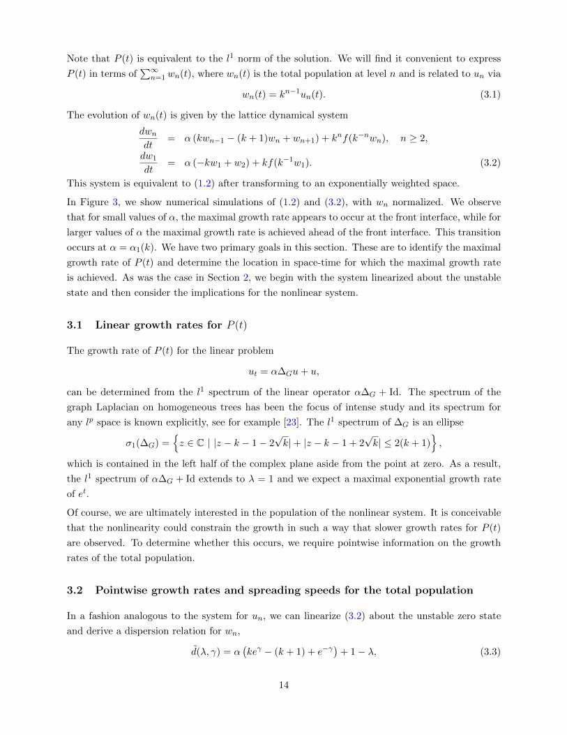
In Figure 3, we show numerical simulations of (1.2) and (3.2), with wn normalized. We observe

that for small values of α, the maximal growth rate appears to occur at the front interface, while for

larger values of α the maximal growth rate is achieved ahead of the front interface. This transition

occurs at α = α1(k). We have two primary goals in this section. These are to identify the maximal

growth rate of P (t) and determine the location in space-time for which the maximal growth rate

is achieved. As was the case in Section 2, we begin with the system linearized about the unstable

state and then consider the implications for the nonlinear system.

3.1 Linear growth rates for P (t)

The growth rate of P (t) for the linear problem

ut = α∆Gu+ u,

can be determined from the l1 spectrum of the linear operator α∆G + Id. The spectrum of the

graph Laplacian on homogeneous trees has been the focus of intense study and its spectrum for

any lp space is known explicitly, see for example [23]. The l1 spectrum of ∆G is an ellipse

σ1(∆G) ={z ∈ C | |z − k − 1− 2

√k|+ |z − k − 1 + 2

√k| ≤ 2(k + 1)

},

which is contained in the left half of the complex plane aside from the point at zero. As a result,

the l1 spectrum of α∆G + Id extends to λ = 1 and we expect a maximal exponential growth rate

of et.

Of course, we are ultimately interested in the population of the nonlinear system. It is conceivable

that the nonlinearity could constrain the growth in such a way that slower growth rates for P (t)

are observed. To determine whether this occurs, we require pointwise information on the growth

rates of the total population.

3.2 Pointwise growth rates and spreading speeds for the total population

In a fashion analogous to the system for un, we can linearize (3.2) about the unstable zero state

and derive a dispersion relation for wn,

d(λ, γ) = α(keγ − (k + 1) + e−γ

)+ 1− λ, (3.3)

14

as well as the equivalent dispersion relation in a co-moving frame ds(λ, γ) = d(λ+ sγ, γ). We again

remark that transforming from un to wn amounts to transforming un to a weighted space. Any

pinched double root (λ∗, γ∗) of the dispersion relation ds(λ, γ) corresponds to a pinched double root

of the dispersion relation ds for (λ, γ) = (λ∗ + s log k, γ∗ − log k); see the following calculation

(ds(λ

∗, γ∗)

∂γds(λ∗, γ∗)

)=

(α(eγ

∗ − k − 1 + ke−γ∗)

+ 1− sγ∗ − λ∗

α(eγ

∗ − ke−γ∗)− s

)

=

(α(keγ

∗−log k − k − 1 + e−γ∗+log k

)+ 1− s(γ∗ − log k)− s log k − λ∗

α(keγ

∗−log k − e−γ∗+log k)− s

)

=

(ds(λ

∗ + s log k, γ∗ − log k)

∂γ ds(λ∗ + s log k, γ∗ − log k)

)Recall that the λ∗ value gives the pointwise growth rate of the solution in a frame moving with

speed s. The decay (growth) rate of any pinched double root for the local population un(t) is thus

increased by s log(k) in the weighted space. Thus, pointwise growth rates of wn may be positive

even when growth rates for un are negative. We have the following.

Lemma 3.1. The linear growth rate is maximized in a frame moving at speed

s∗ = α(k − 1),

i.e. at the u-group velocity of the mode e−n log k.

Proof. Note that γ = 0 and λ = 1 is always a root of the dispersion relation, i.e. d(1, 0) = 0. In

the original frame of reference, this does not correspond to a pinched double root since ∂γ d(1, 0) =

α(1 − k) 6= 0. However, passing to a frame moving with speed s∗ we find ds∗(1, 0) = 0 and

∂γ ds∗(1, 0) = 0.

Remark 3.2. Lemma 3.1 states that the maximal growth rate of a linear problem in an exponen-

tially weighted space occurs on a ray in space-time moving with the group velocity of the exponential

weight. This is a general fact and there are several alternative avenues by which to verify the

statement of Lemma 3.1. Similar results are often obtained by a asymptotic analysis of the Green’s

function via stationary phase. In the context of a homogeneous tree, this fact can be verified from

a direct analysis of the heat kernel, see for example [11, 12]. For the case of parabolic partial

differential equations, this was shown in Lemma 6.3 of [19]. Finally, we mention [18], where the

appearance of pointwise instabilities when transforming to weighted spaces leads to some unexpected

spreading speeds in a system of coupled Fisher-KPP equations.

We now compare the speed s∗ to the linear spreading speed slin and make the the following obser-

vations,

• For α = α1, the maximal growth rate is realized at the linear spreading speed; that is, s∗ = s1

15

• For α < α1 we have that s∗ < slin, while s∗ > slin for α > α1.

These observations lead us to conjecture that the the population grows fastest when s∗ > slin

since in this regime the maximal growth rate is achieved ahead of the front interface where the

nonlinearity is negligible.

3.3 Growth rates in the nonlinear problem

We return our attention to the full nonlinear system and study the growth rate of the total popula-

tion. We expect that the growth rates predicted by the linearized system to place an upper bound

on the growth rates in the nonlinear system.

A key distinction is made between α < α1(k) and α > α1(k). For α below the l1 critical value, the

maximal linear growth rate at level n is achieved in a frame of reference that propagates slower

than the linear spreading speed. In view of Theorem 1, this means that the invasion speed of the

species exceeds s∗. Furthermore, since γlin > log k we expect the mass in the system to be added

at the front interface. The dynamics of the total population can then be approximated by

P (t) ≈∞∑n=1

kn−1 min{1, e−γlin(n−slint)}.

When γlin > log(k) then this sum converges and we expect

P (t) ≈bslintc∑n=1

kn−1 ≈ kslint − 1

k − 1.

Therefore, we expect a maximal growth rate of elog(k)slint when γlin > log(k). Note that for α1, it

is true that log(k)s1 = 1.

For α > α1(k), the speed s∗ exceeds that of slin and therefore the maximal linear growth rate

is achieved ahead of the front interface. Since the solution un(t) is pointwise close to zero in

this region, we expect that the linear dynamics remain valid here and that P (t) ≈ Cet for these

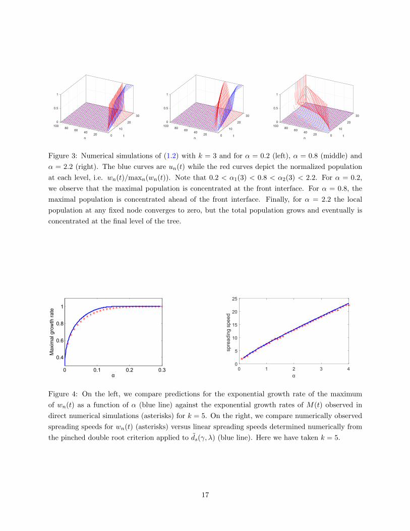
parameter values. This is confirmed in numerical simulations, see Figure 4.

4 Erdos-Renyi random graphs

We now turn our attention to more complicated network topologies. We will use the analytical

results obtained for the homogeneous tree to make predictions for the dynamics of the Fisher-KPP

where G is an Erdos-Renyi random graph. These predictions will then be compared to observations

based upon numerical simulations.

The analysis performed on the homogeneous trees leads us to make two qualitative predictions for

more general networks. First, based upon the leading order independence of the linear spreading

speed on the degree of the tree, we expect that for α asymptotically small the pointwise dynamics

16

30

200

t

10080 10

n

6040

0.5

20 0

1

30

200

t

10080 10

n

6040

0.5

20 0

1

30

200

t

10080 10

n

6040

0.5

20 0

1

Figure 3: Numerical simulations of (1.2) with k = 3 and for α = 0.2 (left), α = 0.8 (middle) and

α = 2.2 (right). The blue curves are un(t) while the red curves depict the normalized population

at each level, i.e. wn(t)/maxn(wn(t)). Note that 0.2 < α1(3) < 0.8 < α2(3) < 2.2. For α = 0.2,

we observe that the maximal population is concentrated at the front interface. For α = 0.8, the

maximal population is concentrated ahead of the front interface. Finally, for α = 2.2 the local

population at any fixed node converges to zero, but the total population grows and eventually is

concentrated at the final level of the tree.

0 0.1 0.2 0.3

0.4

0.6

0.8

1

α

Max

imal

gro

wth

rat

e

0 1 2 3 4

α

0

5

10

15

20

25

spre

adin

g sp

eed

Figure 4: On the left, we compare predictions for the exponential growth rate of the maximum

of wn(t) as a function of α (blue line) against the exponential growth rates of M(t) observed in

direct numerical simulations (asterisks) for k = 5. On the right, we compare numerically observed

spreading speeds for wn(t) (asterisks) versus linear spreading speeds determined numerically from

the pinched double root criterion applied to ds(γ, λ) (blue line). Here we have taken k = 5.

17

of the general system should be well approximated by a finite tree where the only relevant feature is

the distance of a node from the location of initiation. Second, based upon our analysis in Section 3

we expect sub-linear growth rates for the total population for α small.

We first review the Erdos-Renyi random graph model [15]. Let N denote the total number of nodes

in the graph and select some p ∈ (0, 1). Erdos-Renyi random graphs are constructed by assigning

edges to the graph with fixed probability p. We are interested in the case where N � 1 and the

expected degree of each node kER + 1 = Np is small. We select one node at random and call that

node the root. We denote the solution at that node u1(t) and consider (1.1) with u1(0) = 1 and

zero initial condition at every other node.

Several factors motivate our choice of Erdos-Renyi random graphs for study. Notable among these

factors is their prevalence and popularity in the literature. However, another important factor is the

informal observation that Erdos-Renyi random graphs with small p appear locally tree-like: each

node is connected roughly kER + 1 other nodes, which in turn will each be connected to roughly

kER which are themselves not connected with high probability. We refer the reader to [4, 14] and

the reference therein for more rigorous studies of Erdos-Renyi graphs.

We construct networks with size ranging from N = 60, 000 to N = 500, 000, see [2], and vary the

expected degree from three (kER = 2) to sixteen (kER = 15). Note that for the small p values

considered here, the constructed networks are disconnected with probability one. Therefore, when

we discuss the network dynamics below we always restrict our attention to the largest connected

component. Numerically, solutions are computed using explicit Euler with timestep ∆t = .0025.

Changing the timestep did not significantly alter the results.

4.1 Pointwise dynamics: arrival times

In this section, we focus on the pointwise dynamics of the system and describe numerical results

characterizing the spreading speed on random graphs of Erdos Reyni type.

For finite graphs the only stable steady state is the uniform state at one. We assign to each node

a label i ∈ {1, 2, . . . , N}. Let d(i, j) be the shortest distance along the network between nodes i

and j. Denote the node where the species is initialized as i = 1 and specify initial conditions where

u1(0) = 1 and uj(0) = 0 for all j 6= 1. The primary descriptor of the dynamics in this situation is

τi, the arrival time at node i ∈ V , defined as

τi = mint≥0

ui(t) > κ,

for some threshold 0 < κ < 1.

Arrival times as a function of the distance from the initial node are plotted in Figure 5. For very

small α, we observe a strong linear relationship between the arrival time and distance from the

node i = 1. As α is increased this linear relationship becomes less apparent.

18

We will compute the mean arrival time at level l,

Ml =1

Nl

∑i∈V d(i,1)=l

τi.

Based upon this data we find a best fit linear regression line as follows. In order to minimize the

effect of initial transients or boundary effects, we consider only those Ml corresponding to distances

greater than two from the initial node or less than two from the furthest node. A linear regression

is then computed and the reciprocal of the slope is called the numerically observed mean spreading

speed. These regression lines are shown in green in the Figure 5 with green asterisks denoting Ml.

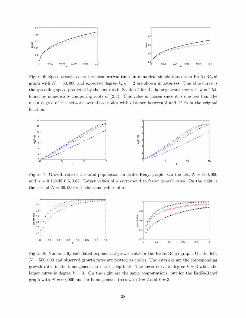
Mean spreading speeds are computed and plotted in Figure 6. We compare these speeds to spreading

speeds on homogeneous trees computed in Section 2. Before drawing any conclusions, some remarks

regarding the relationship between random graphs and regular trees are in order. Important in any

comparison of spreading speeds in the random graph and the homogeneous tree is a selection of

a value of k to be used for comparison. This choice is not obvious, nor is it clear that one such

k will be sufficient. For large Erdos-Renyi graphs, the average degree in the graph will converge

to kER + 1 as N → ∞. At the same time, however, if kER is small then the Erdos-Renyi graph

will be disconnected with probability one. Within the largest connected component the average

degree will exceed kER + 1. The simplest choice is then to take k to be the average degree of all

nodes over which the linear regression is computed. With this choice, the observed and theoretical

speeds are close, however the linear spreading speed consistently overestimates the observed mean

spreading speed. This discrepancy could be due to several factors including the heterogeneity of

the network. However, we also note that in the system (1.2) it takes some time for initial data to

converge to a traveling front and even then the convergence is notoriously slow [5]. As a result, it

is perhaps unrealistic to expect that spreading speeds measured directly in numerical simulations

on the random graph to match exactly with predictions from the linear spreading speed.

We comment briefly on the dynamics for large values of α. For α sufficiently large the first arrival

times cease to be monotonic with respect to distance from the original node. For even larger

values of α the arrival time for most nodes on the graph is approximately constant. This is to be

expected. For α sufficiently large the dominant eigenvalue of the linearization about zero is one,

whose eigenvector is the constant vector ~1. Projecting the initial condition onto this vector we

expect leading order dynamics

u(t) ∼ 1

Net~1,

from which we find a homogeneous arrival time that scales with logN . This is consistent with the

timescale observed for large values of α.

4.2 Aggregate dynamics: population growth rate

We now investigate the exponential growth rate of the total population for (1.1) for Erdos-Renyi

random graphs. We compare these growth rates to those observed on the homogeneous tree.

19

The logarithm of the total population is shown in Figure 7. After an initial transient, the growth

rate appears to be roughly linear corresponding to exponential growth. We measure this growth

rate and compare it to similar computations in the homogeneous tree.

As was the case for the pointwise analysis, an immediate challenge lies in determining the precise

value of k to use in the comparison to the homogeneous tree. Given the variation in the average

degrees across levels of the network, we instead compare numerically observed growth rates in the

random graphs with observed growth rates in homogeneous trees that we expect to provide bounds

on the total growth rate. The results of these simulations are depicted in Figure 8.

Remark 4.1. Population growth rates for the Fisher-KPP equation on Erdos-Renyi random graphs

were also studied in [9]. Recall that sub-linear growth rates were found for the homogeneous tree;

see Section 3.3 where sub-linear growth rates are explained by the existence of finite mass traveling

fronts. We suggest the same mechanism is at play for Erdos-Renyi random graphs although we

do not pursue making this mathematically rigorous. We also note that the analysis on the tree

suggests a growth rate that scales with slin(α) log(k) for small α, which for small α has leading order

asymptotic expansion of − log(α) log(k). This should be contrasted with the polynomial scaling of

the exponential growth rate with respect to α suggested in [9].

5 Discussion and outlook for future work

In this paper, we studied the dynamics of the Fisher-KPP equation defined on homogeneous trees

and Erdos-Reyni random graphs. For the homogeneous tree we study traveling fronts and spreading

speeds. We find that these fronts are linearly determined and propagate at the linear spreading

speed. An interesting property is that these speeds are non-monotone with respect to the diffusion

parameter and eventually become zero. Therefore, for values of α > α2 the solution converges

pointwise exponentially fast to zero. We find that the critical point of the linear spreading speed at

α = α1 occurs for the parameter value where the maximal linear growth rate of the total population

in the network occurs at the linear spreading speed. For larger values of α the front is slowed due

to some fraction of the population escaping down the graph. The increased mobility of the species

allows the population to explore nodes with only small concentrations of the species where the local

growth rate is maximal.

An interesting feature of the linear spreading speed is that it is independent of the degree of the

nodes in the network in the asymptotic limit as α→ 0. This suggested that the spreading properties

observed in the homogeneous tree should be present in random graphs and explored this for the

case of random networks of Erdos-Reyni type. For α asymptotically small, we observed traveling

fronts and characterized their speed. It was also the case that the exponential growth rate of the

population was less than the maximal growth rate of one and bounded this growth rate by the

corresponding growth rate on the homogeneous tree.

Erdos-Reyni graphs are known to share a close relationship to trees. It would be interesting to

20

extend the results here to different, more realistic, random networks such as small world [30] or

scale free networks [1]. The independence of the spreading speed on the degree for small α suggests

that one should continue to observe traveling fronts on these more general networks that are well

approximated by the lattice Fisher-KPP equation. The situation is more complicated for larger

values of α where the heterogeneity of the network can not be denied. It would be interesting to

characterize whether critical diffusion rates analogous to α1 and α2 for these more general classes

of graphs. Example 2.4 gives some indication that the effect of heterogeneity can be quite severe

and so we expect that analysis of these systems would require a more general approach.

Acknowledgements

Portions of this research were initiated as part of a summer undergraduate research program at

George Mason University as part of the EXTREEMS-QED program (NSF-DMS-1407087). MH is

grateful to Robert Truong for insightful discussions related to this project. MH received partial

support from the National Science Foundation through grant NSF-DMS-1516155.

A Proof of Theorem 1

In this section, we prove Theorem 1. The proof relies on the existence of a comparison principle

for (1.2).

Proposition A.1. Suppose that there exists functions un(t) and un(t) such that 0 ≤ un(0) ≤un(0) ≤ 1. Furthermore suppose that for all t ≥ 0 and all n ≥ 2 we have

u′n ≥ α (un−1 − (k + 1)un + kun+1)− f(un)

u′n ≤ α(un−1 − (k + 1)un + kun+1

)− f(un),

while for n = 1,

u′1 ≥ α (−ku1 + ku2)− f(u1)

u′1 ≤ α (−ku1 + ku2)− f(u1).

Then for all t ≥ 0 we have that

0 ≤ un(t) ≤ un(t) ≤ 1.

We refer the reader to [10] for a proof of the comparison principle in a setting similar to the one

here.

We now proceed to the proof of Theorem 1. We find it convenient to break the analysis according

to whether α < α2 or α > α2.

21

Case I: α < α2(k)

Lemma A.2. Let γ > 0 such that senv(γ) > 0. Consider any α < α2. Then

un(t) = min{1, Ce−γ(n−senv(γ)t)},

is a super-solution for all n ∈ N, any C > 1 and all t ≥ 0.

Proof. We need to show that for n ≥ 2

N(un) = u′n − α (un−1 − (k + 1)un + kun+1)− un − (f(un)− un) ≥ 0.

Since the constant 1 is a solution of (1.2), it is by definition a super-solution and N(1) = 0. The

exponential term propagates at the envelope velocity of the mode γ. We recall that

α(eγ − k − 1 + ke−γ

)− γsenv(γ) + 1 = 0.

As a result, we have that the linear terms in N(un) are zero and

N(Ce−γ(n−senv(γ)t)

)= − (f(un)− un) ,

which is positive by the KPP assumption f(u) < f ′(0)u. Thus, the exponential is a super-solution

for all n ≥ 2. Since C > 1, the super-solution is always one at the root and we have that u is a

super-solution.

We now turn our attention to the construction of sub-solutions. Let 0 < µ < 1 and consider the

linear equationdφndt

= α (φn−1 − (k + 1)φn + kφn+1) + µφn.

Exponential solutions e−γ(n−st) are obtained for γ and s satisfying the following equation

α(eγ − (k + 1) + ke−γ

)− sγ + µ = 0. (A.1)

For each µ, there exists sµ such that (A.1) has no real solutions for s < sµ. Let γµ ∈ C be a

complex solution. Then let

φµ(y) = eγµy + c.c., (A.2)

where c.c. denotes the complex conjugate and fix a < b such that φ(y) > 0 for y ∈ (a, b) and

φ(a) = φ(b) = 0. We use these functions to construct sub-solutions in the following Lemma.

Lemma A.3. Fix α < α2(k) and let s < slin. Let µ < 1 such that s < sµ. Then there exists

T > 0, a function φµ(y) and an ε∗ such that

un(t) =

{εφµ(n− st) a ≤ n− st ≤ b

0 else(A.3)

is a sub-solution for all 0 < ε < ε∗ and for all t > T .

22

Proof. For s < slin, select µ < 1 so that s < sµ and consider the function φµ in (A.2) whose support

is the interval [a+ st, b+ st]. Let T be sufficiently large so that sT + a > 1. Now consider

N(un) = u′n − α (un−1 − (k + 1)un + kun+1)− un − (f(un)− un) .

We find

N(un) = −εφ(n− st)(1− µ) + (εφ(n− st)− f(εφ(n− st))) .

For u small, there exists a C > 0 such that −Cu2 < f(u) − u. Let ε be sufficiently small so that

this bound holds for (A.3). Then

N(un) < εφ(n− st) (−(1− µ) + Cεφ(n− st)) ,

and if we restrict

ε <1− µ

C maxy∈[a,b] φ(y),

then N(un) < 0 and un is a sub-solution.

Case II: α > α2(k) For α > α2, we only concern ourselves with the establishment of super-

solutions.

Lemma A.4. Consider any α > α2. Let γ > 0 such that senv(γ) < 0. Then

un(t) = e−γ(n−senv(γ)t),

is a super-solution for all n ∈ N and all t ≥ 0.

Proof. We follow the proof of Lemma A.4 and compute N(un). The calculation is exactly the same,

aside from the root. There we calculate

N(u1) =(senv(γ)γ − α(k + 1)(−1 + e−γ)− 1

)e−γ(1−senv(γ)t) − (f(un)− un)

= αe−γ(1−senv(γ)t)(eγ − e−γ

)− (f(un)− un) .

Since both terms are positive, we have that N(u1) is positive as well and the proof is completed.

We now prove Theorem 1. The claim of pointwise convergence for α > α2(k) follows from

Lemma A.4 and the fact that senv(γ) < 0. Consider then α < α2. Here, we have that the

linear spreading speed is positive and obtained for some value of slin with selected decay rate γlin.

Then since C > 1 in Lemma A.2 we have that un(0) ≥ un(0). Due to the comparison principle, this

relationship holds for all time and we obtain an upper bound on the location of the invasion point:

κ(t) ≤ slin(α)t. To obtain a lower bound, we consider the sub-solutions constructed in Lemma A.3.

Select s < slin(α) and consider un from Lemma A.3. Let t1 > T . By the maximum principle,

we have that un(t1) > 0 for all n ∈ N. Since un(t1) is compactly supported, we can select ε > 0

sufficiently small such that un(t1) ≤ un(t1). Therefore, we have that κ(t) ≥ st. This holds for any

s < slin(α) and we find slin(α) ≤ ssel ≤ slin(α) and Theorem 1 is established.

23

References

[1] A.-L. Barabasi and R. Albert. Emergence of scaling in random networks. science,

286(5439):509–512, 1999.

[2] V. Batagelj and U. Brandes. Efficient generation of large random networks. Phys. Rev. E,

71:036113, Mar 2005.

[3] A. Bers. Space-time evolution of plasma instabilities-absolute and convective. In A. A. Galeev

& R. N. Sudan, editor, Basic Plasma Physics: Selected Chapters, Handbook of Plasma Physics,

Volume 1, pages 451–517, 1984.

[4] B. Bollobas. Random graphs, volume 73 of Cambridge Studies in Advanced Mathematics.

Cambridge University Press, Cambridge, second edition, 2001.

[5] M. Bramson. Convergence of solutions of the Kolmogorov equation to travelling waves. Mem.

Amer. Math. Soc., 44(285):iv+190, 1983.

[6] L. Brevdo and T. J. Bridges. Absolute and convective instabilities of spatially periodic flows.

Philos. Trans. Roy. Soc. London Ser. A, 354(1710):1027–1064, 1996.

[7] R. J. Briggs. Electron-Stream Interaction with Plasmas. MIT Press, Cambridge, 1964.

[8] D. Brockmann and D. Helbing. The hidden geometry of complex, network-driven contagion

phenomena. Science, 342(6164):1337–1342, 2013.

[9] R. Burioni, S. Chibbaro, D. Vergni, and A. Vulpiani. Reaction spreading on graphs. Phys.

Rev. E, 86:055101, Nov 2012.

[10] X. Chen. Existence, uniqueness, and asymptotic stability of traveling waves in nonlocal evo-

lution equations. Adv. Differential Equations, 2(1):125–160, 1997.

[11] G. Chinta, J. Jorgenson, and A. Karlsson. Heat kernels on regular graphs and generalized

Ihara zeta function formulas. Monatsh. Math., 178(2):171–190, 2015.

[12] F. Chung and S.-T. Yau. Coverings, heat kernels and spanning trees. Electron. J. Combin.,

6:Research Paper 12, 21 pp. (electronic), 1999.

[13] V. Colizza, R. Pastor-Satorras, and A. Vespignani. Reaction–diffusion processes and metapop-

ulation models in heterogeneous networks. Nat Phys, 3:276–282, Jan. 2007.

[14] R. Durrett. Random graph dynamics, volume 20 of Cambridge Series in Statistical and Prob-

abilistic Mathematics. Cambridge University Press, Cambridge, 2007.

[15] P. Erdos and A. Renyi. On random graphs. I. Publ. Math. Debrecen, 6:290–297, 1959.

24

[16] R. A. Fisher. The wave of advance of advantageous genes. Annals of Human Genetics,

7(4):355–369, 1937.

[17] J. Hindes, S. Singh, C. R. Myers, and D. J. Schneider. Epidemic fronts in complex networks

with metapopulation structure. Phys. Rev. E, 88:012809, Jul 2013.

[18] M. Holzer. A proof of anomalous invasion speeds in a system of coupled Fisher-KPP equations.

Discrete Contin. Dyn. Syst., 36(4):2069–2084, 2016.

[19] M. Holzer and A. Scheel. Criteria for pointwise growth and their role in invasion processes. J.

Nonlinear Sci., 24(4):661–709, 2014.

[20] A. Kolmogorov, I. Petrovskii, and N. Piscounov. Etude de l’equation de la diffusion avec

croissance de la quantite’ de matiere et son application a un probleme biologique. Moscow

Univ. Math. Bull., 1:1–25, 1937.

[21] N. E. Kouvaris, H. Kori, and A. S. Mikhailov. Traveling and pinned fronts in bistable reaction-

diffusion systems on networks. PLoS ONE, 7(9):1–12, 09 2012.

[22] H. Matano, F. Punzo, and A. Tesei. Front propagation for nonlinear diffusion equations on

the hyperbolic space. J. Eur. Math. Soc. (JEMS), 17(5):1199–1227, 2015.

[23] B. Mohar and W. Woess. A survey on spectra of infinite graphs. Bull. London Math. Soc.,

21(3):209–234, 1989.

[24] M. E. J. Newman. The structure and function of complex networks. SIAM Review, 45(2):167–

256, 2003.

[25] M. A. Porter and J. P. Gleeson. Dynamical systems on networks, volume 4 of Frontiers in

Applied Dynamical Systems: Reviews and Tutorials. Springer, Cham, 2016. A tutorial.

[26] B. Sandstede and A. Scheel. Absolute and convective instabilities of waves on unbounded and

large bounded domains. Phys. D, 145(3-4):233–277, 2000.

[27] S. H. Strogatz. Exploring complex networks. Nature, 410(6825):268–276, Mar. 2001.

[28] W. van Saarloos. Front propagation into unstable states. Physics Reports, 386(2-6):29 – 222,

2003.

[29] A. Vespignani. Modelling dynamical processes in complex socio-technical systems. Nature

Physics, 8:32–39, 2012.

[30] D. J. Watts and S. H. Strogatz. Collective dynamics of ‘small-world’networks. nature,

393(6684):440–442, 1998.

[31] H. F. Weinberger. Long-time behavior of a class of biological models. SIAM Journal on

Mathematical Analysis, 13(3):353–396, 1982.

25

[32] B. Zinner, G. Harris, and W. Hudson. Traveling wavefronts for the discrete Fisher’s equation.

J. Differential Equations, 105(1):46–62, 1993.

26

(a) α = 0.001. (b) α = 0.01. (c) α = 0.1.

(d) α = 0.2. (e) α = 0.5. (f) α = 1.0.

(g) α = 2.0. (h) α = 4.0.

Figure 5: Arrival times for an Erdos Reyni graph with N = 60, 000 and expected degree kER = 2.

Various values of α are considered. In green is the best fit linear approximation for the mean arrival

times for nodes with distance between 3 and 12 from the initial location.

27

0 0.002 0.004 0.006 0.008 0.01

0.2

0.25

0.3

0.35

0.4

α

speed

0 0.02 0.04 0.06 0.08 0.10.2

0.4

0.6

0.8

1

α

speed

Figure 6: Speed associated to the mean arrival times in numerical simulations on an Erdos Reyni

graph with N = 60, 000 and expected degree kER = 2 are shown in asterisks. The blue curve is

the spreading speed predicted by the analysis in Section 2 for the homogeneous tree with k = 2.54,

found by numerically computing roots of (2.3). This value is chosen since it is one less than the

mean degree of the network over those nodes with distance between 3 and 12 from the original

location.

0 5 10 150

2

4

6

8

10

12

14

t

log(P(t))

0 5 10 150

2

4

6

8

10

12

t

log(P(t))

Figure 7: Growth rate of the total population for Erdos-Renyi graph. On the left, N = 500, 000

and α = 0.1, 0.35, 0.6, 0.85. Larger values of α correspond to faster growth rates. On the right is

the case of N = 60, 000 with the same values of α.

0 0.1 0.2 0.3 0.4 0.5 0.6 0.7

0.4

0.5

0.6

0.7

0.8

0.9

1

α

grow

th r

ate

0 0.2 0.4 0.6 0.8 1α

0.2

0.4

0.6

0.8

1

grow

th r

ate

Figure 8: Numerically calculated exponential growth rate for the Erdos-Renyi graph. On the left,

N = 500, 000 and observed growth rates are plotted as circles. The asterisks are the corresponding

growth rates in the homogeneous tree with depth 13. The lower curve is degree k = 3 while the

larger curve is degree k = 4. On the right are the same computations, but for the Erdos-Renyi

graph with N = 60, 000 and for homogeneous trees with k = 2 and k = 3.

28