INVASE: I WISE VARIABLE SELECTION US ING N

Published as a conference paper at ICLR 2019

INVASE: INSTANCE-WISE VARIABLE SELECTION US-ING NEURAL NETWORKS

Jinsung YoonDepartment of Electrical and Computer EngineeringUCLA, California, [email protected]

James JordonEngineering Science DepartmentUniversity of Oxford, [email protected]

Mihaela van der SchaarUniversity of Cambridge, UKDepartment of Electrical and Computer Engineering, UCLA, California, USAAlan Turing Institute, London, [email protected]

ABSTRACT

The advent of big data brings with it data with more and more dimensions and thusa growing need to be able to efficiently select which features to use for a varietyof problems. While global feature selection has been a well-studied problem forquite some time, only recently has the paradigm of instance-wise feature selectionbeen developed. In this paper, we propose a new instance-wise feature selectionmethod, which we term INVASE. INVASE consists of 3 neural networks, a selec-tor network, a predictor network and a baseline network which are used to trainthe selector network using the actor-critic methodology. Using this methodology,INVASE is capable of flexibly discovering feature subsets of a different size foreach instance, which is a key limitation of existing state-of-the-art methods. Wedemonstrate through a mixture of synthetic and real data experiments that IN-VASE significantly outperforms state-of-the-art benchmarks.

1 INTRODUCTION

High-dimensional data is becoming more readily available, and it brings with it a growing need to beable to efficiently select which features to use for a variety of problems. When doing predictions, itis well known that using too many variables with too few samples can lead to overfitting, which cansignificantly hinder the performance of predictive models. In the realm of interpretability, the largedimensionality of the data is often too much information to present to a human who may be using themachine learning model as a support system. Understanding which features are most relevant to anoutcome or to a model output is an important first step in improving predictions and interpretabilityand many works exist that tackle feature selection on a global level. However, in the heterogeneousdata we typically encounter, the prediction made by a model (and indeed the true label) may rely on adifferent subset of the features for different subgroups within the data [14]. In this paper we proposea novel instance-wise feature selection method, INVASE (INstance-wise VAriable SElection), whichattempts to learn which subset of the features is relevant for each sample, allowing us to display theminimal information required to explain each prediction and also to reduce overfitting of predictivemodels.

Discovering a global subset of relevant features for a particular task is a well-studied problem andthere are several existing methods for solving it such as Sequential Correlation Feature Selection[11], Mutual Information Feature Selection [21], Knockoff models [3], and more [10; 16]. However,global feature selection suffers from a key limitation - the features discovered by global featureselection are the same for all samples. In many cases, in particular when populations are highlyheterogeneous, the relevant features may differ across samples [33; 32]. For instance, differentpatient subgroups have different relevant features for predicting heart failure [14]. Instance-wisefeature selection methods such as [4; 27] instead try to discover the features that are relevant for

1


each sample. When the goal is to provide an interpretable explanation of the predictions made, akey challenge is in ensuring that we do not over-explain by providing too much information (i.e.choosing too many features). Naturally, by performing feature selection on an individualized levelwe are able to select features that are more relevant to each sample, rather than having to choosethe top k features globally, which may not explain the predictions for some samples very well, butsimply perform well on average across all samples.

In this paper, we propose a novel instance-wise feature selection method which we term INVASE.We draw influence from actor-critic models [22] to solve the problem of backpropagating throughsubset sampling. Our model consists of 3 neural networks: a selector network, a predictor networkand a baseline network. During training, each of these are trained iteratively, with the selectornetwork being trained to minimize a Kullback-Leibler (KL) divergence between the full conditionaldistribution and the selected-features-only conditional distribution of the outcome. Our model iscapable of discovering a different number of relevant variables for each sample which is a keylimitation in existing instance-wise approaches (such as [4]). We show significant improvementsover the state-of-the-art in both synthetic data and real-word data in terms of true positive rates,false discovery rates, and show better predictive performance with respect to several predictionmetrics. Our model can also be easily extended to handle both continuous and discrete outputs andtime-series inputs (see the Appendix for details).

1.1 RELATED WORKS

There are many existing works on global variable selection (see [10] for a good summary paper).[21] and [11] use max-dependency min-redundancy criteria [17] with mutual information and Pear-son correlation, respectively. [3] uses multiple hypothesis testing for global variable selection. Asnoted above, these global selection methods are not capable of learning sample-specific relevance.

Instance-wise variable selection is also closely related to model interpretation methods. Some pre-vious works are based on backpropagation from the output of the predictive model to the inputvariables [29]. DeepLIFT [27] decomposes the output of the neural network on a reference input tocompute the contribution of each input variable. However, both methods need white-box access tothe pre-trained predictive models to compute the gradient and decomposition. [2] approximates thepredictive models using a Parzen window approximator when there is only black-box access to thepredictive models. Some other works are based on input perturbation such as [1], [15], [30] and [5].[18] uses Shapley values to compute the variable importance, and [24] uses locally linear models toexplain the linear dependency for each sample. [19] tries to interpret tree ensemble models usingShapley values but cannot generalize to other predictive models such as neural networks.

Our work is most closely related to L2X (Learning to Explain) [4]. However, there are 3 key dif-ferences between our work and theirs. In L2X, they try to maximize a lower bound of the mutualinformation between the target Y and the selected input variables XS . In contrast, we try to mini-mize the KL divergence between the conditional distributions Y |X and Y |XS . In order to be able tobackpropagate through subset sampling, L2X use the Gumbel-softmax trick [13] to approximatelydiscretize the continuous outputs of the neural network. In our work, we use methods from actor-critic models [22] to bypass backpropagation through the sampling and instead use the predictornetwork to provide a reward to the selector network. Finally, due to the Gumbel-softmax used inL2X, the number of variables to be detected must be fixed in advance and is necessarily the same forevery sample. The actor-critic methodology used in our model has no such limitations and so we areable to flexibly select a different number of relevant variables for each sample and instead inducesparsity using an l0 penalty term. In fact, using the actor-critic methodology allows us to directlyuse the l0 penalty term (which is not differentiable and therefore not practical to use in general). Asummary table highlighting the key features of all of the related works can be found in the Appendix.

2 PROBLEM FORMULATION

Let X = X1 × ... × Xd be a d-dimensional feature space and Y = {1, ..., c} be a discrete labelspace1. Let X = (X1, ..., Xd) ∈ X and Y ∈ Y be random variables with joint density (or mass)p and marginal densities (or masses) pX and pY respectively. We will refer to s ∈ {0, 1}d as the

1In this paper we focus on classification; we discuss an extension of our model to regression in the Appendix.

2


selection vector, where si = 1 will indicate that variable i is selected, and si = 0 will indicatethat variable i is not selected. Let ∗ be any point not in any of the spaces X1, ...,Xd and defineX ∗i = Xi ∪{∗} and X ∗ = X ∗1 × ...×X ∗d . Given x ∈ X we will write x(s) to denote the suppressedfeature vector defined by

x(s)i =

{xi if si = 1

∗ if si = 0

so that ∗ represents that a feature is not selected.

In the global feature selection literature, the goal is to find the smallest s (i.e. the one with fewest 1s)such that E(Y |X(s)) = E(Y |X), or equivalently such that the conditional distribution of Y givenX(s) is the same as Y given all of X. Note that this definition is given fully in terms of randomvariables, rather than realizations of those random variables.

In contrast, our problem necessarily needs to be defined in terms of realizations since we are aimingto select features for a given realization. We will write x to denote realizations of the randomvariable X. Then we formalize our problem as one of finding a selector function, S : X → {0, 1}dsuch that for almost every x ∈ X (w.r.t. pX ) we have

(Y |X(S(x)) = x(S(x)))d.= (Y |X = x) (1)

where d.= denotes equality in distribution and S(x) is minimal (i.e. fewest 1s) such that (1) holds.

We suppose that we have a dataset D = {(xj , yj)}nj=1 consisting of n i.i.d. realizations of thepair (X, Y ).2 Note that Y can be viewed as having either come from a dataset, in which case theproblem is of selecting predictive features, or as having come from a predictive model, in whichcase the problem is of explaining the model’s predictions.

2.1 OPTIMIZATION PROBLEM

In order to learn a suitable selector function, we transform the constraint (1) into a soft constraintusing the Kullback-Leibler (KL) divergence which, for random variables W and V with densitiespW and pV is defined as

KL(W ||V ) = E[log

(pW (W )

pV (W )

)].

We define the following loss for our selector function S

L(S) = Ex∼pX

[KL(Y |X = x||Y |X(S(x)) = x(S(x))) + λ||S(x)||

](2)

where || · || simply denotes the number of non-zero entries of a vector (or equivalently in this case,the number of 1s) and λ is a hyper-parameter that trades off between the constraint in (1) and thenumber of selected features. The KL divergence in (2) can be rewritten as

KL(Y |X = x||Y |X(S(x)) = x(S(x))) = Ey∼Y |X=x

[log

(pY (y|x)

pY (y|x(S(x)))

)]= Ey∼Y |X=x

[log(pY (y|x))− log(pY (y|x(S(x))))

]=

∫YpY (y|x)

[log(pY (y|x))− log(pY (y|x(S(x))))

]dy

where pY (·|·) denotes the appropriate conditional densities of Y . We will write

l(x, s) =

∫YpY (y|x)

[log(pY (y|x))− log(pY (y|x(s)))

]dy (3)

so that our final loss can be written as

L(S) = Ex∼pX [l(x, S(x)) + λ||S(x)||] (4)

where || · || denotes the l0 (pseudo-)norm.2We will occasionally abuse notation and write yi to denote the ith element of the one-hot encoding of y,

though the context should make it clear when this is the case.

3


3 PROPOSED MODEL

There are two main challenges in minimizing the loss in (4). First, the output space of the selectorfunction ({0, 1}d) is large - its size increases exponentially with the dimension of the feature space;thus a complete search is impractical in high dimensional settings (and it should be noted that it isin high dimensional settings where feature selection is most necessary). Second, we do not haveaccess to the densities pY (·|x(S(x))) and pY (y|x) required to compute (4).

3.1 LOSS ESTIMATION

To approximate the densities in (3), we introduce a pair of functions fφ : X ∗ × {0, 1}d → [0, 1]c

parametrized by φ and fγ : X → [0, 1]c parametrized by γ that will estimate pY (·|x(S(x))) andpY (·|x) respectively.

3.1.1 PREDICTOR NETWORK

We refer to fφ as the predictor network. This will take as input a suppressed3 feature vector x(s)

and its corresponding selection vector s and will output a probability distribution (using a softmaxlayer) over the c-dimensional output space.

fφ is trained to minimize the cross entropy loss given by

l1(φ) = −E(x,y)∼p,s∼πθ(x,·)

[ c∑i=1

yi log(fφi (x(s), s))]

where yi is the ith component of the one-hot encoding of y and πθ is the distribution induced byour selector network which will be defined in the following section. fφ is implemented as a fullyconnected neural network4.

3.1.2 BASELINE NETWORK

We refer to fγ as the baseline network, which is standard in the actor-critic literature for variancereduction. fγ is implemented as a fully connected neural network and is trained to minimize

l3(γ) = −E(x,y)∼p

[ c∑i=1

yi log(fγi (x))].

For fixed φ, γ we define our loss estimator, l, by

l(x, s) = −

[c∑i=1

yi log(fφi (x(s), s))−c∑i=1

yi log(fγi (x))

]. (5)

3.2 SELECTOR FUNCTION OPTIMIZATION

We approximate the selector function S : X → {0, 1}d by using a single neural network, Sθ : X →[0, 1]d parameterized by weights θ, that outputs a probability for selecting each feature (i.e. the ithcomponent of Sθ(x) will denote the probability with which we select the ith feature). The selectornetwork induces a probability distribution over the selection space ({0, 1}d), with the probability ofa given joint selection vector s ∈ {0, 1}d being given by5

πθ(x, s) = Πdi=1S

θi (x)si(1− Sθi (x))1−si .

3When implemented we set ∗ = 0 and include the selection vector to differentiate this from the case xi = 0.4fφ, fγ and Sθ could also be implemented as CNNs or RNNs, when appropriate.5Note that, when d is large, this becomes vanishingly small, however, πθ appears in our loss only via its log

and so in practice this is not a problem.

4


Selector Network𝑥

𝑥

𝑥

…

𝑥

FeaturesSelection

Probability

RandomSampler

Predictor Network

��

��

…

��

Predictor Loss(Cross Entropy)⊚

Back-propagation

Baseline Network

𝑝

𝑝

…

𝑝

0

1

…

0

Loss Difference

𝑝

𝑝

𝑝

…

𝑝

1

0

1

…

0

𝑥

𝑥

𝑥

…

𝑥Selection

Selected Features

Label

Baseline Loss(Cross Entropy)

Label estimation

Back-propagation

𝑥

𝑥

𝑥

…

𝑥

Features Label estimation

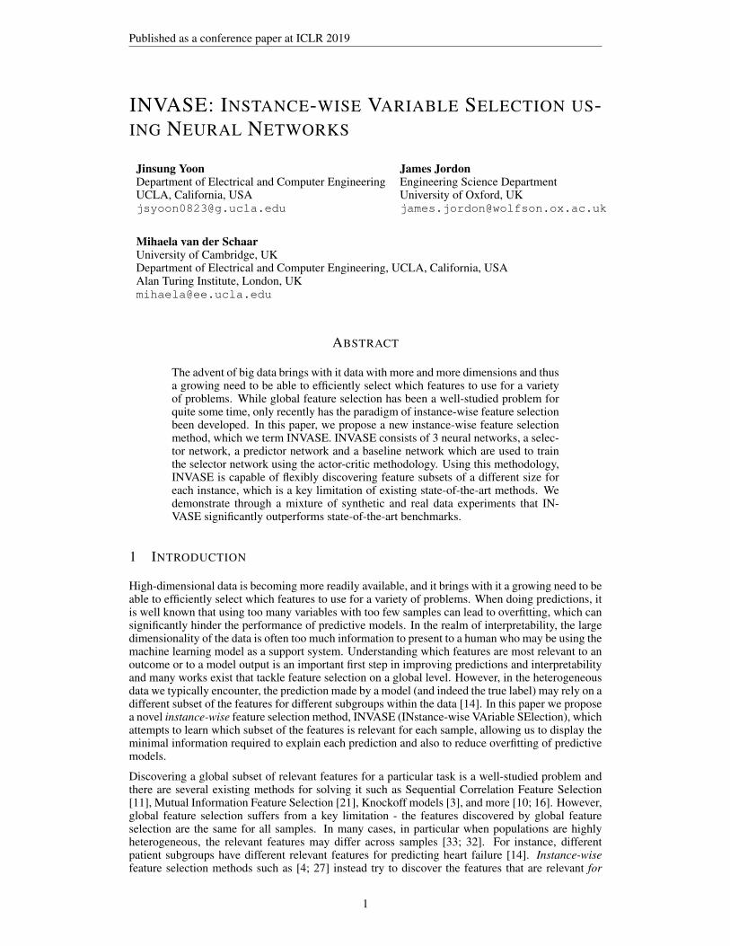
Element-wise product

Figure 1: Block diagram of INVASE. Instances are fed into the selector network which outputsa vector of selection probabilities. The selection vector is then sampled according to these proba-bilities. The predictor network then receives the selected features and makes a prediction and thebaseline network is given the entire feature vector and makes a prediction. Each of these networksare trained using backpropagation using the real label. The loss of the baseline network is thensubtracted from the prediction network’s loss and this is used to update the selector network.

Using this, we define the following loss for our selector network

l2(θ) = E(x,y)∼p

[Es∼πθ(x,·)

[l(x, s) + λ||s||0

]]=

∫X×Y

p(x, y)

∑s∈{0,1}d

πθ(x, s)(l(x, s) + λ||s||0

) dxdy.

Taking the gradient of this loss with respect to θ gives us

∇θl2(θ) =

∫X×Y

p(x, y)

∑s∈{0,1}d

∇θπθ(x, s)(l(x, s) + λ||s||0

) dxdy

=

∫X×Y

p(x, y)

∑s∈{0,1}d

∇θπθ(x, s)πθ(x, s)

πθ(x, s)(l(x, s) + λ||s||0

) dxdy

=

∫X×Y

p(x, y)

∑s∈{0,1}d

∇θ log πθ(x, s)πθ(x, s)(l(x, s) + λ||s||0

) dxdy

= E(x,y)∼p

[Es∼πθ(x,·)

[(l(x, s) + λ||s||0

)∇θ log πθ(x, s)

]].

We update each of Sθ, fφ and fγ iteratively using stochastic gradient descent. Pseudo-code ofINVASE is given in Algorithm 1 and a block representation of INVASE can be found in Fig. 1.

4 EXPERIMENTS

In this section, we quantitatively evaluate INVASE against various state-of-the-art benchmarks onboth synthetic and real-world datasets. We evaluate our performance both at identifying groundtruth relevance and at enhancing predictions. We compare our model with 4 global variable selectionmodels: Knockoffs [3], Tree Ensembles (Tree) [7], Sequential Correlation Feature Selection (SCFS)[11], and LASSO regularized linear model; and 3 instance-wise feature selection methods: L2X

5


Algorithm 1 Pseudo-code of INVASE

1: Inputs: learning rates α, β > 0, mini-batch size nmb > 0, dataset D2: Initialize parameters θ, φ, γ3: while Converge do4: Sample a mini-batch from the dataset (xj , yj)

nmbj=1 ∼ D

5: for j = 1, ..., nmb do6: Calculate selection probabilities

(pj1, ..., pjd)← Sθ(xj)

7: Sample selection vector8: for i = 1, ..., d do

sji ∼ Ber(pji )

9: Calculate loss

lj(xj , sj)← −

[c∑i=1

yji log(fφi (x(sj)j , sj))−

c∑i=1

yji log(fγi (xj))

]

10: Update the selector network parameters θ

θ ← θ − α 1

nmb

nmb∑j=1

(lj(xj , sj) + λ||sj ||

)∇θ log πθ(xj , sj)

11: Update the predictor network parameters φ

φ← φ− β 1

nmb

nmb∑j=1

c∑i=1

yji ×∇φ log(fφi (x(sj)j , sj))

12: Update the baseline network parameters γ

γ ← γ − β 1

nmb

nmb∑j=1

c∑i=1

yji ×∇γ log(fγi (xj))

[4], LIME [24], and Shapley [18]. The details of benchmark implementation can be found in theappendix. Implementation of INVASE can be found at https://github.com/jsyoon0823/INVASE.

4.1 SYNTHETIC DATA EXPERIMENTS

4.1.1 EXPERIMENTAL SETTINGS

For our first set of experiments, we use the same synthetic data generation models as in L2X [4]. Theinput features are generated from an 11-dimensional67 Gaussian distribution with no correlationsacross the features (X ∼ N (0, I)). The label Y is sampled as a Bernoulli random variable withP(Y = 1|X) = 1

1+logit(X) , where logit(X) is varied to create 3 different synthetic datasets:

• Syn1: exp(X1X2)

• Syn2: exp(∑6i=3X

2i − 4)

• Syn3: −10× sin 2X7 + 2|X8|+X9 + exp(−X10)

6In L2X they use a 10-dimensional Gaussian, we introduce X11 to act as a “switch” to create instance-wiserelevance. Experiments where instead the “switch” variable is one ofX1, ..., X10 can be found in the appendix.

7We also perform experiments using 100 features in the Appendix to demonstrate the scalability of ourmethod.

6

https://github.com/jsyoon0823/INVASE

https://github.com/jsyoon0823/INVASE


In each of these datasets, the label depends on the same subset of features for every sample. To high-light the capability of INVASE to detect instance-wise dependence, we generate 3 further syntheticdatasets as follows:

• Syn4: If X11 < 0, logit follows Syn1, otherwise, logit follows Syn2.• Syn5: If X11 < 0, logit follows Syn1, otherwise, logit follows Syn3.• Syn6: If X11 < 0, logit follows Syn2, otherwise, logit follows Syn3.

Note that in Syn4 and Syn5, the number of relevant features is different for different samples.

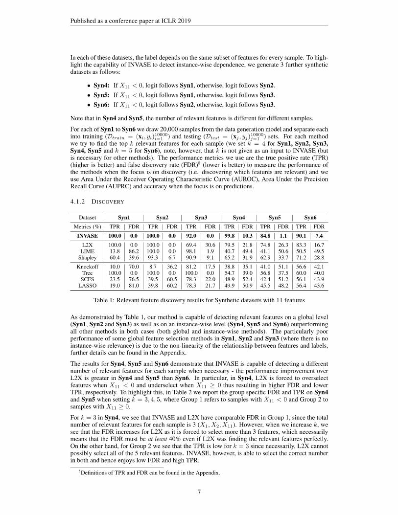
For each of Syn1 to Syn6 we draw 20,000 samples from the data generation model and separate eachinto training (Dtrain = (xi, yi)10000i=1 ) and testing (Dtest = (xj , yj)10000j=1 ) sets. For each methodwe try to find the top k relevant features for each sample (we set k = 4 for Syn1, Syn2, Syn3,Syn4, Syn5 and k = 5 for Syn6), note, however, that k is not given as an input to INVASE (butis necessary for other methods). The performance metrics we use are the true positive rate (TPR)(higher is better) and false discovery rate (FDR)8 (lower is better) to measure the performance ofthe methods when the focus is on discovery (i.e. discovering which features are relevant) and weuse Area Under the Receiver Operating Characteristic Curve (AUROC), Area Under the PrecisionRecall Curve (AUPRC) and accuracy when the focus is on predictions.

4.1.2 DISCOVERY

Dataset Syn1 Syn2 Syn3 Syn4 Syn5 Syn6Metrics (%) TPR FDR TPR FDR TPR FDR TPR FDR TPR FDR TPR FDR

INVASE 100.0 0.0 100.0 0.0 92.0 0.0 99.8 10.3 84.8 1.1 90.1 7.4L2X 100.0 0.0 100.0 0.0 69.4 30.6 79.5 21.8 74.8 26.3 83.3 16.7

LIME 13.8 86.2 100.0 0.0 98.1 1.9 40.7 49.4 41.1 50.6 50.5 49.5Shapley 60.4 39.6 93.3 6.7 90.9 9.1 65.2 31.9 62.9 33.7 71.2 28.8

Knockoff 10.0 70.0 8.7 36.2 81.2 17.5 38.8 35.1 41.0 51.1 56.6 42.1Tree 100.0 0.0 100.0 0.0 100.0 0.0 54.7 39.0 56.8 37.5 60.0 40.0

SCFS 23.5 76.5 39.5 60.5 78.3 22.0 48.9 52.4 42.4 51.2 56.1 43.9LASSO 19.0 81.0 39.8 60.2 78.3 21.7 49.9 50.9 45.5 48.2 56.4 43.6

Table 1: Relevant feature discovery results for Synthetic datasets with 11 features

As demonstrated by Table 1, our method is capable of detecting relevant features on a global level(Syn1, Syn2 and Syn3) as well as on an instance-wise level (Syn4, Syn5 and Syn6) outperformingall other methods in both cases (both global and instance-wise methods). The particularly poorperformance of some global feature selection methods in Syn1, Syn2 and Syn3 (where there is noinstance-wise relevance) is due to the non-linearity of the relationship between features and labels,further details can be found in the Appendix.

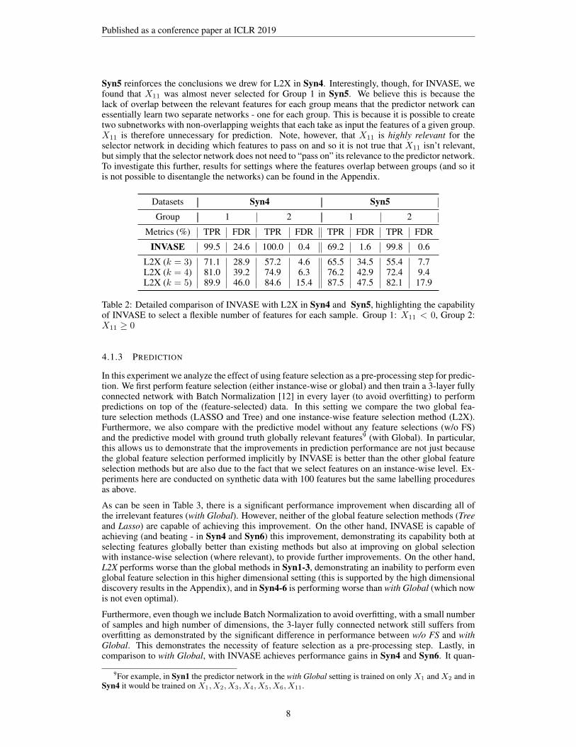
The results for Syn4, Syn5 and Syn6 demonstrate that INVASE is capable of detecting a differentnumber of relevant features for each sample when necessary - the performance improvement overL2X is greater in Syn4 and Syn5 than Syn6. In particular, in Syn4, L2X is forced to overselectfeatures when X11 < 0 and underselect when X11 ≥ 0 thus resulting in higher FDR and lowerTPR, respectively. To highlight this, in Table 2 we report the group specific FDR and TPR on Syn4and Syn5 when setting k = 3, 4, 5, where Group 1 refers to samples with X11 < 0 and Group 2 tosamples with X11 ≥ 0.

For k = 3 in Syn4, we see that INVASE and L2X have comparable FDR in Group 1, since the totalnumber of relevant features for each sample is 3 (X1, X2, X11). However, when we increase k, wesee that the FDR increases for L2X as it is forced to select more than 3 features, which necessarilymeans that the FDR must be at least 40% even if L2X was finding the relevant features perfectly.On the other hand, for Group 2 we see that the TPR is low for k = 3 since necessarily, L2X cannotpossibly select all of the 5 relevant features. INVASE, however, is able to select the correct numberin both and hence enjoys low FDR and high TPR.

8Definitions of TPR and FDR can be found in the Appendix.

7


Syn5 reinforces the conclusions we drew for L2X in Syn4. Interestingly, though, for INVASE, wefound that X11 was almost never selected for Group 1 in Syn5. We believe this is because thelack of overlap between the relevant features for each group means that the predictor network canessentially learn two separate networks - one for each group. This is because it is possible to createtwo subnetworks with non-overlapping weights that each take as input the features of a given group.X11 is therefore unnecessary for prediction. Note, however, that X11 is highly relevant for theselector network in deciding which features to pass on and so it is not true that X11 isn’t relevant,but simply that the selector network does not need to “pass on” its relevance to the predictor network.To investigate this further, results for settings where the features overlap between groups (and so itis not possible to disentangle the networks) can be found in the Appendix.

Datasets Syn4 Syn5Group 1 2 1 2

Metrics (%) TPR FDR TPR FDR TPR FDR TPR FDR

INVASE 99.5 24.6 100.0 0.4 69.2 1.6 99.8 0.6

L2X (k = 3) 71.1 28.9 57.2 4.6 65.5 34.5 55.4 7.7L2X (k = 4) 81.0 39.2 74.9 6.3 76.2 42.9 72.4 9.4L2X (k = 5) 89.9 46.0 84.6 15.4 87.5 47.5 82.1 17.9

Table 2: Detailed comparison of INVASE with L2X in Syn4 and Syn5, highlighting the capabilityof INVASE to select a flexible number of features for each sample. Group 1: X11 < 0, Group 2:X11 ≥ 0

4.1.3 PREDICTION

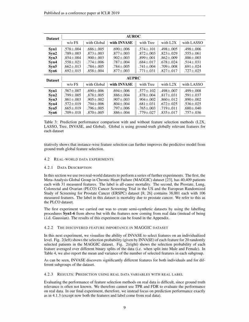
In this experiment we analyze the effect of using feature selection as a pre-processing step for predic-tion. We first perform feature selection (either instance-wise or global) and then train a 3-layer fullyconnected network with Batch Normalization [12] in every layer (to avoid overfitting) to performpredictions on top of the (feature-selected) data. In this setting we compare the two global fea-ture selection methods (LASSO and Tree) and one instance-wise feature selection method (L2X).Furthermore, we also compare with the predictive model without any feature selections (w/o FS)and the predictive model with ground truth globally relevant features9 (with Global). In particular,this allows us to demonstrate that the improvements in prediction performance are not just becausethe global feature selection performed implicitly by INVASE is better than the other global featureselection methods but are also due to the fact that we select features on an instance-wise level. Ex-periments here are conducted on synthetic data with 100 features but the same labelling proceduresas above.

As can be seen in Table 3, there is a significant performance improvement when discarding all ofthe irrelevant features (with Global). However, neither of the global feature selection methods (Treeand Lasso) are capable of achieving this improvement. On the other hand, INVASE is capable ofachieving (and beating - in Syn4 and Syn6) this improvement, demonstrating its capability both atselecting features globally better than existing methods but also at improving on global selectionwith instance-wise selection (where relevant), to provide further improvements. On the other hand,L2X performs worse than the global methods in Syn1-3, demonstrating an inability to perform evenglobal feature selection in this higher dimensional setting (this is supported by the high dimensionaldiscovery results in the Appendix), and in Syn4-6 is performing worse than with Global (which nowis not even optimal).

Furthermore, even though we include Batch Normalization to avoid overfitting, with a small numberof samples and high number of dimensions, the 3-layer fully connected network still suffers fromoverfitting as demonstrated by the significant difference in performance between w/o FS and withGlobal. This demonstrates the necessity of feature selection as a pre-processing step. Lastly, incomparison to with Global, with INVASE achieves performance gains in Syn4 and Syn6. It quan-

9For example, in Syn1 the predictor network in the with Global setting is trained on only X1 and X2 and inSyn4 it would be trained on X1, X2, X3, X4, X5, X6, X11.

8


Dataset AUROCw/o FS with Global with INVASE with Tree with L2X with LASSO

Syn1 .578±.004 .686±.005 .690±.006 .574±.101 .498±.005 .498±.006Syn2 .789±.003 .873±.003 .877±.003 .872±.003 .823±.029 .555±.061Syn3 .854±.004 .900±.003 .902±.003 .899±.001 .862±.009 .886±.003Syn4 .558±.021 .774±.006 .787±.004 .684±.017 .678±.024 .514±.031Syn5 .662±.013 .784±.005 .784±.005 .741±.004 .709±.008 .691±.024Syn6 .692±.015 .858±.004 .877±.003 .771±.031 .827±.017 .727±.025

Dataset AUPRCw/o FS with Global with INVASE with Tree with L2X with LASSO

Syn1 .567±.007 .690±.006 .694±.006 .577±.102 .498±.007 .499±.008Syn2 .799±.005 .878±.005 .886±.004 .878±.004 .817±.031 .591±.037Syn3 .861±.003 .905±.002 .907±.003 .904±.002 .860±.012 .890±.002Syn4 .572±.019 .794±.006 .804±.004 .681±.031 .672±.025 .536±.025Syn5 .665±.019 .796±.005 .797±.006 .765±.003 .719±.011 .680±.040Syn6 .709±.018 .870±.005 .886±.004 .779±.027 .835±.017 .757±.036

Table 3: Prediction performance comparison with and without feature selection methods (L2X,LASSO, Tree, INVASE, and Global). Global is using ground-truth globally relevant features foreach dataset

titatively shows that instance-wise feature selection can further improves the predictive model fromground truth global feature selection.

4.2 REAL-WORLD DATA EXPERIMENTS

4.2.1 DATA DESCRIPTION

In this section we use two real-world datasets to perform a series of further experiments. The first, theMeta-Analysis Global Group in Chronic Heart Failure (MAGGIC) dataset [23], has 40,409 patientseach with 31 measured features. The label is all-cause mortality. The second, the Prostate, Lung,Colorectal and Ovarian (PLCO) Cancer Screening Trial in the US and the European RandomizedStudy of Screening for Prostate Cancer (ERSPC) dataset [8; 26] contains 38,001 each with 106measured features. The label in this dataset is mortality due to prostate cancer. We refer to this asthe PLCO dataset.

The first experiment we carried out was to create semi-synthetic datasets by using the labellingprocedures Syn1-6 from above but with the features now coming from real data (instead of beingi.i.d. Gaussian). The results of this experiment can be found in the Appendix.

4.2.2 THE DISCOVERED FEATURE IMPORTANCE IN MAGGIC DATASET

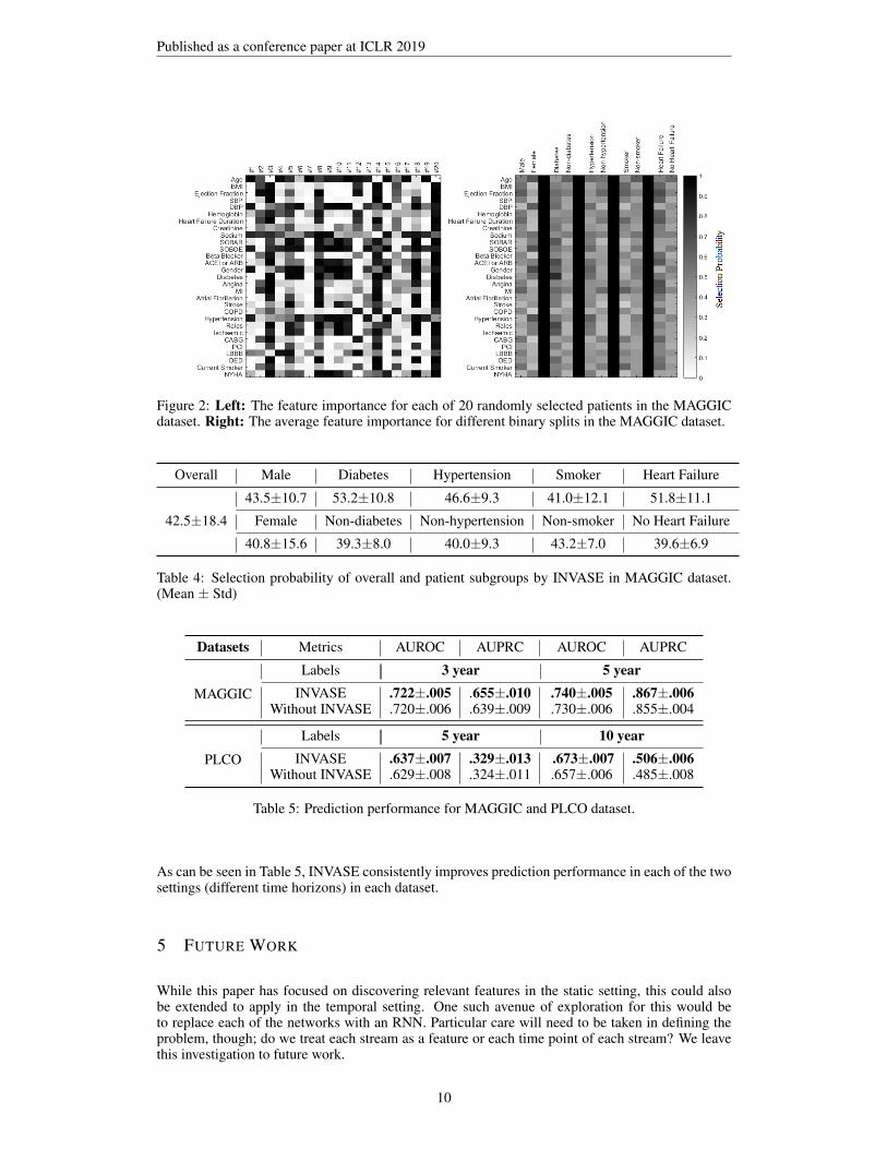
In this next experiment, we visualize the ability of INVASE to select features on an individualizedlevel. Fig. 2(left) shows the selection probability (given by INVASE) of each feature for 20 randomlyselected patients in the MAGGIC dataset. Fig. 2(right) shows the selection probability of eachfeature averaged over different binary splits of the data (i.e. when split into Male and Female). InTable 4, we also report the mean and variance of the number of selected features in each subgroup.

As can be seen, INVASE discovers significantly different features for both individuals and for dif-ferent subgroups of the dataset.

4.2.3 RESULTS: PREDICTION USING REAL DATA VARIABLES WITH REAL LABEL

Evaluating the performance of feature selection methods on real data is difficult, since ground truthrelevance is often not known. We therefore cannot use TPR and FDR to evaluate the performanceon real data. In our final experiment, therefore, we instead focus on prediction performance exactlyas in 4.1.3 (except now both the features and label come from real data).

9


Figure 2: Left: The feature importance for each of 20 randomly selected patients in the MAGGICdataset. Right: The average feature importance for different binary splits in the MAGGIC dataset.

Overall Male Diabetes Hypertension Smoker Heart Failure

43.5±10.7 53.2±10.8 46.6±9.3 41.0±12.1 51.8±11.1

42.5±18.4 Female Non-diabetes Non-hypertension Non-smoker No Heart Failure

40.8±15.6 39.3±8.0 40.0±9.3 43.2±7.0 39.6±6.9

Table 4: Selection probability of overall and patient subgroups by INVASE in MAGGIC dataset.(Mean ± Std)

Datasets Metrics AUROC AUPRC AUROC AUPRC

MAGGIC

Labels 3 year 5 yearINVASE .722±.005 .655±.010 .740±.005 .867±.006

Without INVASE .720±.006 .639±.009 .730±.006 .855±.004

PLCO

Labels 5 year 10 yearINVASE .637±.007 .329±.013 .673±.007 .506±.006

Without INVASE .629±.008 .324±.011 .657±.006 .485±.008

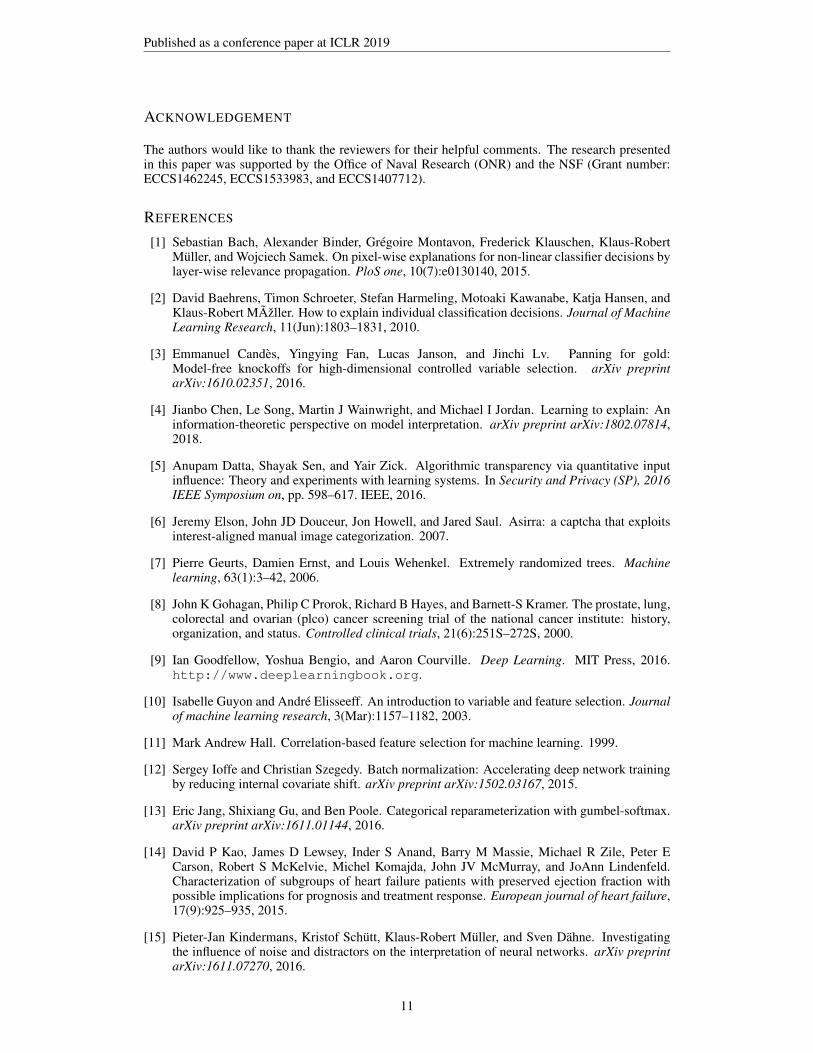
Table 5: Prediction performance for MAGGIC and PLCO dataset.

As can be seen in Table 5, INVASE consistently improves prediction performance in each of the twosettings (different time horizons) in each dataset.

5 FUTURE WORK

While this paper has focused on discovering relevant features in the static setting, this could alsobe extended to apply in the temporal setting. One such avenue of exploration for this would beto replace each of the networks with an RNN. Particular care will need to be taken in defining theproblem, though; do we treat each stream as a feature or each time point of each stream? We leavethis investigation to future work.

10


ACKNOWLEDGEMENT

The authors would like to thank the reviewers for their helpful comments. The research presentedin this paper was supported by the Office of Naval Research (ONR) and the NSF (Grant number:ECCS1462245, ECCS1533983, and ECCS1407712).

REFERENCES

[1] Sebastian Bach, Alexander Binder, Gregoire Montavon, Frederick Klauschen, Klaus-RobertMuller, and Wojciech Samek. On pixel-wise explanations for non-linear classifier decisions bylayer-wise relevance propagation. PloS one, 10(7):e0130140, 2015.

[2] David Baehrens, Timon Schroeter, Stefan Harmeling, Motoaki Kawanabe, Katja Hansen, andKlaus-Robert MAzller. How to explain individual classification decisions. Journal of MachineLearning Research, 11(Jun):1803–1831, 2010.

[3] Emmanuel Candes, Yingying Fan, Lucas Janson, and Jinchi Lv. Panning for gold:Model-free knockoffs for high-dimensional controlled variable selection. arXiv preprintarXiv:1610.02351, 2016.

[4] Jianbo Chen, Le Song, Martin J Wainwright, and Michael I Jordan. Learning to explain: Aninformation-theoretic perspective on model interpretation. arXiv preprint arXiv:1802.07814,2018.

[5] Anupam Datta, Shayak Sen, and Yair Zick. Algorithmic transparency via quantitative inputinfluence: Theory and experiments with learning systems. In Security and Privacy (SP), 2016IEEE Symposium on, pp. 598–617. IEEE, 2016.

[6] Jeremy Elson, John JD Douceur, Jon Howell, and Jared Saul. Asirra: a captcha that exploitsinterest-aligned manual image categorization. 2007.

[7] Pierre Geurts, Damien Ernst, and Louis Wehenkel. Extremely randomized trees. Machinelearning, 63(1):3–42, 2006.

[8] John K Gohagan, Philip C Prorok, Richard B Hayes, and Barnett-S Kramer. The prostate, lung,colorectal and ovarian (plco) cancer screening trial of the national cancer institute: history,organization, and status. Controlled clinical trials, 21(6):251S–272S, 2000.

[9] Ian Goodfellow, Yoshua Bengio, and Aaron Courville. Deep Learning. MIT Press, 2016.http://www.deeplearningbook.org.

[10] Isabelle Guyon and Andre Elisseeff. An introduction to variable and feature selection. Journalof machine learning research, 3(Mar):1157–1182, 2003.

[11] Mark Andrew Hall. Correlation-based feature selection for machine learning. 1999.

[12] Sergey Ioffe and Christian Szegedy. Batch normalization: Accelerating deep network trainingby reducing internal covariate shift. arXiv preprint arXiv:1502.03167, 2015.

[13] Eric Jang, Shixiang Gu, and Ben Poole. Categorical reparameterization with gumbel-softmax.arXiv preprint arXiv:1611.01144, 2016.

[14] David P Kao, James D Lewsey, Inder S Anand, Barry M Massie, Michael R Zile, Peter ECarson, Robert S McKelvie, Michel Komajda, John JV McMurray, and JoAnn Lindenfeld.Characterization of subgroups of heart failure patients with preserved ejection fraction withpossible implications for prognosis and treatment response. European journal of heart failure,17(9):925–935, 2015.

[15] Pieter-Jan Kindermans, Kristof Schutt, Klaus-Robert Muller, and Sven Dahne. Investigatingthe influence of noise and distractors on the interpretation of neural networks. arXiv preprintarXiv:1611.07270, 2016.

11

http://www.deeplearningbook.org


[16] Kenji Kira and Larry A Rendell. A practical approach to feature selection. In Machine Learn-ing Proceedings 1992, pp. 249–256. Elsevier, 1992.

[17] Yaojin Lin, Qinghua Hu, Jinghua Liu, and Jie Duan. Multi-label feature selection based onmax-dependency and min-redundancy. Neurocomputing, 168:92–103, 2015.

[18] Scott M Lundberg and Su-In Lee. A unified approach to interpreting model predictions. InAdvances in Neural Information Processing Systems, pp. 4765–4774, 2017.

[19] Scott M Lundberg, Gabriel G Erion, and Su-In Lee. Consistent individualized feature attribu-tion for tree ensembles. arXiv preprint arXiv:1802.03888, 2018.

[20] Omkar M Parkhi, Andrea Vedaldi, Andrew Zisserman, and CV Jawahar. Cats and dogs. InComputer Vision and Pattern Recognition (CVPR), 2012 IEEE Conference on, pp. 3498–3505.IEEE, 2012.

[21] Hanchuan Peng, Fuhui Long, and Chris Ding. Feature selection based on mutual informa-tion criteria of max-dependency, max-relevance, and min-redundancy. IEEE Transactions onpattern analysis and machine intelligence, 27(8):1226–1238, 2005.

[22] Jan Peters and Stefan Schaal. Natural actor-critic. Neurocomputing, 71(7-9):1180–1190, 2008.

[23] Stuart J Pocock, Cono A Ariti, John JV McMurray, Aldo Maggioni, Lars Køber, Iain B Squire,Karl Swedberg, Joanna Dobson, Katrina K Poppe, Gillian A Whalley, et al. Predicting survivalin heart failure: a risk score based on 39 372 patients from 30 studies. European heart journal,34(19):1404–1413, 2012.

[24] Marco Tulio Ribeiro, Sameer Singh, and Carlos Guestrin. Why should i trust you?: Explainingthe predictions of any classifier. In Proceedings of the 22nd ACM SIGKDD internationalconference on knowledge discovery and data mining, pp. 1135–1144. ACM, 2016.

[25] Olaf Ronneberger, Philipp Fischer, and Thomas Brox. U-net: Convolutional networks forbiomedical image segmentation. In International Conference on Medical image computingand computer-assisted intervention, pp. 234–241. Springer, 2015.

[26] Fritz H Schroder, Jonas Hugosson, Monique J Roobol, Teuvo LJ Tammela, Stefano Ciatto,Vera Nelen, Maciej Kwiatkowski, Marcos Lujan, Hans Lilja, Marco Zappa, et al. Screen-ing and prostate-cancer mortality in a randomized european study. New England Journal ofMedicine, 360(13):1320–1328, 2009.

[27] Avanti Shrikumar, Peyton Greenside, and Anshul Kundaje. Learning important featuresthrough propagating activation differences. arXiv preprint arXiv:1704.02685, 2017.

[28] Karen Simonyan and Andrew Zisserman. Very deep convolutional networks for large-scaleimage recognition. arXiv preprint arXiv:1409.1556, 2014.

[29] Karen Simonyan, Andrea Vedaldi, and Andrew Zisserman. Deep inside convolutionalnetworks: Visualising image classification models and saliency maps. arXiv preprintarXiv:1312.6034, 2013.

[30] Erik Strumbelj and Igor Kononenko. Explaining prediction models and individual predictionswith feature contributions. Knowledge and information systems, 41(3):647–665, 2014.

[31] Robert Tibshirani. Regression shrinkage and selection via the lasso. Journal of the RoyalStatistical Society. Series B (Methodological), pp. 267–288, 1996.

[32] Jinsung Yoon, William R Zame, Amitava Banerjee, Martin Cadeiras, Ahmed M Alaa, and Mi-haela van der Schaar. Personalized survival predictions via trees of predictors: An applicationto cardiac transplantation. PloS one, 13(3):e0194985, 2018.

[33] Jinsung Yoon, William R Zame, and Mihaela van der Schaar. Tops: Ensemble learning withtrees of predictors. IEEE Transactions on Signal Processing, 66(8):2141–2152, 2018.

12


APPENDIX

SUMMARY OF RELATED WORKS

Key ideas Experiments Global/ Model # of relevantshown Instance-wise agnostic features

SCFS Max-dependency min-redundancy Feature selection Global Yes Not needed[11] criteria with Pearson correlations

MIFS Max-dependency min-redundancy Feature selection Global Yes Not needed[21] criteria with Mutual Information

LASSO Linear regression Feature selection Global Yes Not needed[31] with l1-norm penalty Prediction

Knock-off Comparison between knock-off Feature selection Global Yes Not needed[3] variables and real variables Hypothesis test

L2X Mutual Information maximization Interpretation Instance-wise Yes Should be[4] with Gumbel-softmax given

LIME Locally linear Interpretation Instance-wise Yes Should be[24] approximation given

Shapley Shapley value estimation Feature selection Instance-wise Yes Should be[18] to quantify feature importance given

DeepLIFT Decompose the output of Interpretation Instance-wise No Should be[27] NN on a reference input given

Saliency Backpropagation from the Interpretation Instance-wise No Should be[29] output of the NN to the input given

Tree SHAP Shapley value estimation Interpretation Instance-wise No Should be[19] only for tree-ensemble models given

Pixel-wise Measuring the effects on Interpretation Instance-wise No Should be[1] the output using input perturbation given

INVASE Minimize KL divergence using Feature selectionInstance-wise Yes Not needed(Ours) deep NN influenced by Interpretation

actor-critic models Prediction

Table 6: Summary of the related works. (NN: Neural networks, KL: Kullback-Leibler)

EXTENDING INVASE TO REGRESSION

To extend our model to the setting where Y is continuous (regression problem), we replace theestimated loss with the reconstruction error as follows.

l(x, s) = −||y − fφ(x, s)||2where fφ : X → R is now the (continuous) predictor function trained to minimize the `2-normbetween its outputs and the real labels. As noted in [9], when the distribution of Y given X isGaussian, minimizing the l2-norm is equivalent to minimizing the KL divergence.

DETAILS OF INVASE

In the experiments, the depth of the selector, predictor, and baseline networks is set to 3. The numberof hidden nodes in each layer is d and 2d, respectively. We use either ReLu or SeLu as the activationfunctions of each layer except for the output layer where we use the sigmoid activation function forthe selector network and softmax activation function for the predictor and baseline networks. Thenumber of samples in each mini-batch is 1000 for the selector, predictor, and baseline networks.We use cross-validation to select λ among {0.1, 0.3, 0.5, 1, 2, 5, 10}. We use tensorflow to imple-ment INVASE. The source-code can be found at https://github.com/iclr2018invase/INVASE/.

13

https://github.com/iclr2018invase/INVASE/

https://github.com/iclr2018invase/INVASE/


DETAILS OF BENCHMARKS

We use the following links for the implementations of 7 benchmarks.

• L2X: https://github.com/Jianbo-Lab/L2X• LIME: https://github.com/marcotcr/lime• Shapley: https://github.com/slundberg/shap• Knock-off: http://web.stanford.edu/group/candes/knockoffs/software/knockoff/

• Tree: http://scikit-learn.org/stable/modules/generated/sklearn.ensemble.ExtraTreesClassifier.html

• LASSO: http://scikit-learn.org/stable/modules/linear_model.html#lasso

For L2X, we use the same network settings used in INVASE for fair comparisons. For SCFS, weexplicitly implement from the reference ([11]).

HIGH DIMENSIONAL DISCOVERY

To demonstrate the scalability of our method, we run an experiment in which we increase the totalnumber of features to 100. The features are generated as a 100-dimensional Gaussian with nocorrelations (N (0, I)) and the relationships between features and label remains as in Table 1 in themain manucript (i.e. we are adding 89 additional noisy signals that have no effect on the label).


INVASE 100.0 0.0 100.0 0.0 100.0 0.0 66.3 40.5 73.2 23.7 90.5 15.4L2X 6.1 93.9 81.4 18.6 57.7 42.3 48.5 46.4 35.4 60.8 66.3 33.7

LIME 0.0 100.0 100.0 0.0 92.7 7.3 43.8 47.4 42.3 50.1 50.1 49.9Shapley 4.4 95.6 95.1 4.9 88.8 11.2 50.2 43.4 49.9 44.2 62.5 37.5

Knock off 0.0 64.9 3.7 71.2 74.9 24.9 28.2 59.8 33.1 59.4 46.9 53.0Tree 49.9 50.1 100.0 0.0 100.0 0.0 40.7 49.5 56.7 37.5 58.4 41.6

SCFS 2.5 97.5 5.3 94.7 74.9 25.1 27.0 74.6 30.6 62.1 38.3 61.7LASSO 2.5 97.5 4.0 96.0 75.3 24.7 28.3 73.2 36.0 56.9 45.9 54.1

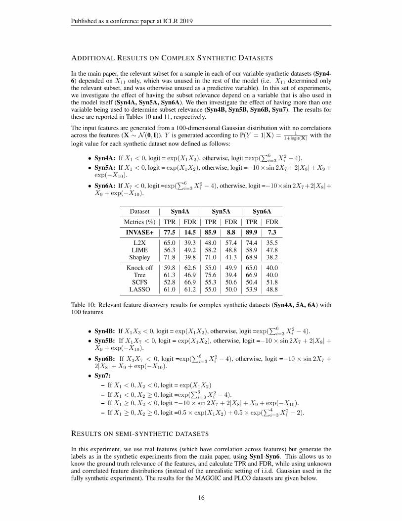
Table 7: Relevant feature discovery for synthetic datasets with 100 features

As can be seen in Table 7, INVASE also works consistently better than all other benchmarks in all 6synthetic datasets in this setting. In fact, we see a significant reduction in performance (compared tothe 11 feature setting) for L2X in Syn1, with the TPR dropping more than 90% leading to an almostcomplete failure of the method to detect any relevant features. In particular, we see that L2X doesnot scale as well as INVASE with the dimensionality of the data, which is particularly limiting for afeature selection method.

We also compare the CPU times of the algorithm for training and testing with other instance-wisefeature selection benchmarks to show the scalability in terms of computational complexity. Ascan be seen in Table 8, INVASE is much faster (10 times) than LIME and Shapley methods andcomparable with L2X; we see that INVASE takes approximately 50% longer to run than L2X,which can be accounted for by the addition of a 3rd network (the baseline network) in INVASE thatis not present in L2X. Note, however, that this baseline network can be trained in parallel with thepredictor network and we believe that doing so would lead to both INVASE and L2X having thesame run-time.

14

https://github.com/Jianbo-Lab/L2X

https://github.com/marcotcr/lime

https://github.com/slundberg/shap

http://web.stanford.edu/group/candes/knockoffs/software/knockoff/

http://web.stanford.edu/group/candes/knockoffs/software/knockoff/

http://scikit-learn.org/stable/modules/generated/sklearn.ensemble.ExtraTreesClassifier.html

http://scikit-learn.org/stable/modules/generated/sklearn.ensemble.ExtraTreesClassifier.html

http://scikit-learn.org/stable/modules/linear_model.html#lasso

http://scikit-learn.org/stable/modules/linear_model.html#lasso


Methods INVASE L2X Shapley LIME

Train 1327.69s 939.82s 12801.21s -Test 0.38s 0.78s 0.06s 18931.98s

Table 8: Comparison of CPU clock time across different instance-wise feature selection methods onaverage across Syn1 to Syn6 with 100 features and 10,000 samples on training/testing, respectively

HYPER-PARAMETER ANALYSIS

In the following experiment, we provide results for various values of the hyper-parameter, λ, in theSyn4, Syn5, and Syn6 100-dimensional setting. Table 9 gives the results in terms of TPR and FDR.Note that in the other experiments, we select the hyper-parameter λ which maximizes the predictoraccuracy in terms of AUROC.

Datasets Syn4 Syn5 Syn6

λ / Metris (%) TPR FDR TPR FDR TPR FDR

0.1 98.0 94.3 90.0 93.4 99.2 92.30.3 93.7 87.9 84.2 88.9 96.9 86.70.5 99.0 43.1 88.3 50.6 99.6 31.71 66.3 40.5 73.2 23.7 90.5 15.42 0.0 0.0 25.4 4.1 67.1 3.65 0.0 0.0 7.5 2.7 7.6 2.5

10 0.0 0.0 0.0 0.0 0.0 0.0

Table 9: Relevant feature discovery results for various values of the hyper-parameter λ in the Syn4,Syn5, and Syn6 100-dimensional setting.

15


ADDITIONAL RESULTS ON COMPLEX SYNTHETIC DATASETS

In the main paper, the relevant subset for a sample in each of our variable synthetic datasets (Syn4-6) depended on X11 only, which was unused in the rest of the model (i.e. X11 determined onlythe relevant subset, and was otherwise unused as a predictive variable). In this set of experiments,we investigate the effect of having the subset relevance depend on a variable that is also used inthe model itself (Syn4A, Syn5A, Syn6A). We then investigate the effect of having more than onevariable being used to determine subset relevance (Syn4B, Syn5B, Syn6B, Syn7). The results forthese are reported in Tables 10 and 11, respectively.

The input features are generated from a 100-dimensional Gaussian distribution with no correlationsacross the features (X ∼ N (0, I)). Y is generated according to P(Y = 1|X) = 1

1+logit(X) with thelogit value for each synthetic dataset now defined as follows:

• Syn4A: If X1 < 0, logit = exp(X1X2), otherwise, logit =exp(∑6i=3X

2i − 4).

• Syn5A: If X1 < 0, logit = exp(X1X2), otherwise, logit =−10× sin 2X7 + 2|X8|+X9 +exp(−X10).

• Syn6A: IfX7 < 0, logit =exp(∑6i=3X

2i − 4), otherwise, logit =−10×sin 2X7+2|X8|+

X9 + exp(−X10).

Dataset Syn4A Syn5A Syn6AMetrics (%) TPR FDR TPR FDR TPR FDR

INVASE+ 77.5 14.5 85.9 8.8 89.9 7.3L2X 65.0 39.3 48.0 57.4 74.4 35.5

LIME 56.3 49.2 58.2 48.8 58.9 47.8Shapley 71.8 39.8 71.0 41.3 68.9 38.2

Knock off 59.8 62.6 55.0 49.9 65.0 40.0Tree 61.3 46.9 75.6 39.4 66.9 40.0

SCFS 52.8 66.9 55.3 50.6 50.4 51.8LASSO 61.0 61.2 55.0 50.0 53.9 48.8

Table 10: Relevant feature discovery results for complex synthetic datasets (Syn4A, 5A, 6A) with100 features

• Syn4B: If X1X3 < 0, logit = exp(X1X2), otherwise, logit =exp(∑6i=3X

2i − 4).

• Syn5B: If X1X7 < 0, logit = exp(X1X2), otherwise, logit =−10 × sin 2X7 + 2|X8| +X9 + exp(−X10).

• Syn6B: If X3X7 < 0, logit =exp(∑6i=3X

2i − 4), otherwise, logit =−10 × sin 2X7 +

2|X8|+X9 + exp(−X10).• Syn7:

– If X1 < 0, X2 < 0, logit = exp(X1X2)

– If X1 < 0, X2 ≥ 0, logit =exp(∑6i=3X

2i − 4).

– If X1 ≥ 0, X2 < 0, logit =−10× sin 2X7 + 2|X8|+X9 + exp(−X10).– If X1 ≥ 0, X2 ≥ 0, logit =0.5× exp(X1X2) + 0.5× exp(

∑4i=3X

2i − 2).

RESULTS ON SEMI-SYNTHETIC DATASETS

In this experiment, we use real features (which have correlation across features) but generate thelabels as in the synthetic experiments from the main paper, using Syn1-Syn6. This allows us toknow the ground truth relevance of the features, and calculate TPR and FDR, while using unknownand correlated feature distributions (instead of the unrealistic setting of i.i.d. Gaussian used in thefully synthetic experiment). The results for the MAGGIC and PLCO datasets are given below.

16


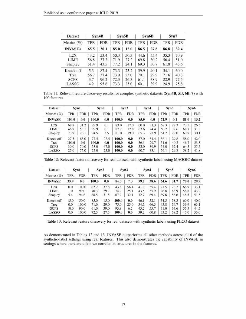
Dataset Syn4B Syn5B Syn6B Syn7Metrics (%) TPR FDR TPR FDR TPR FDR TPR FDR

INVASE+ 65.5 30.1 85.0 15.0 86.5 27.8 86.8 32.4L2X 43.2 53.4 50.3 50.3 44.6 55.4 35.3 70.9

LIME 56.8 37.2 71.9 27.2 69.8 30.2 56.4 51.0Shapley 51.4 43.5 77.2 24.1 69.3 30.7 61.8 45.6

Knock off 5.3 87.4 73.3 25.2 59.9 40.1 54.1 60.0Tree 56.7 37.4 73.9 25.0 70.1 29.9 71.6 40.3

SCFS 3.7 96.2 72.3 26.3 61.1 38.9 22.9 77.5LASSO 4.2 95.6 73.3 25.0 60.1 39.9 24.9 75.8

Table 11: Relevant feature discovery results for complex synthetic datasets (Syn4B, 5B, 6B, 7) with100 features


INVASE 100.0 0.0 100.0 0.0 100.0 0.0 85.9 0.0 72.9 0.1 81.0 13.2L2X 68.8 31.2 99.9 0.1 83.0 17.0 60.0 31.3 68.3 22.3 73.5 26.5

LIME 46.9 53.1 99.9 0.1 87.2 12.8 63.6 24.4 50.2 37.6 68.7 31.3Shapley 73.9 26.1 94.5 5.5 81.0 19.0 65.3 23.9 61.2 29.0 69.9 30.1

Knock off 27.5 65.0 77.5 22.5 100.0 0.0 57.0 34.4 56.1 29.8 58.0 42.0Tree 100.0 0.0 100.0 0.0 100.0 0.0 56.3 29.7 51.6 40.2 46.7 53.3

SCFS 30.0 70.0 53.0 47.0 100.0 0.0 52.0 39.9 54.0 32.4 64.5 35.5LASSO 25.0 75.0 75.0 25.0 100.0 0.0 60.7 33.1 56.1 29.8 58.2 41.8

Table 12: Relevant feature discovery for real datasets with synthetic labels using MAGGIC dataset


INVASE 35.9 0.0 100.0 0.0 84.0 7.0 59.2 38.6 64.6 31.7 70.0 29.9L2X 0.0 100.0 62.2 37.8 43.6 56.4 41.9 55.4 21.5 76.7 66.9 33.1

LIME 1.0 99.0 70.3 29.7 74.9 25.1 43.5 55.9 26.8 68.9 56.8 43.2Shapley 5.4 94.6 68.5 31.5 67.9 32.1 32.7 69.4 39.6 58.6 48.5 51.5

Knock off 15.0 50.0 85.0 15.0 100.0 0.0 46.1 52.1 34.5 58.3 60.0 40.0Tree 0.0 100.0 71.0 29.0 75.0 25.0 34.5 66.3 43.8 54.7 36.9 63.1

SCFS 10.0 90.0 61.0 39.0 93.8 6.2 43.2 55.7 31.0 63.6 55.5 44.5LASSO 0.0 100.0 72.5 27.5 100.0 0.0 39.2 60.8 33.2 68.2 45.0 55.0

Table 13: Relevant feature discovery for real datasets with synthetic labels using PLCO dataset

As demonstrated in Tables 12 and 13, INVASE outperforms all other methods across all 6 of thesynthetic-label settings using real features. This also demonstrates the capability of INVASE insettings where there are unknown correlation structures in the features.

17


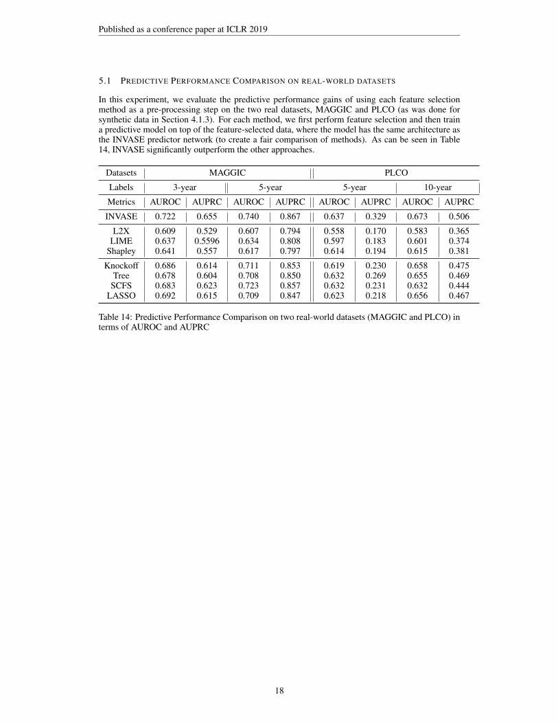
5.1 PREDICTIVE PERFORMANCE COMPARISON ON REAL-WORLD DATASETS

In this experiment, we evaluate the predictive performance gains of using each feature selectionmethod as a pre-processing step on the two real datasets, MAGGIC and PLCO (as was done forsynthetic data in Section 4.1.3). For each method, we first perform feature selection and then traina predictive model on top of the feature-selected data, where the model has the same architecture asthe INVASE predictor network (to create a fair comparison of methods). As can be seen in Table14, INVASE significantly outperform the other approaches.

Datasets MAGGIC PLCO

Labels 3-year 5-year 5-year 10-year

Metrics AUROC AUPRC AUROC AUPRC AUROC AUPRC AUROC AUPRC

INVASE 0.722 0.655 0.740 0.867 0.637 0.329 0.673 0.506

L2X 0.609 0.529 0.607 0.794 0.558 0.170 0.583 0.365LIME 0.637 0.5596 0.634 0.808 0.597 0.183 0.601 0.374

Shapley 0.641 0.557 0.617 0.797 0.614 0.194 0.615 0.381

Knockoff 0.686 0.614 0.711 0.853 0.619 0.230 0.658 0.475Tree 0.678 0.604 0.708 0.850 0.632 0.269 0.655 0.469

SCFS 0.683 0.623 0.723 0.857 0.632 0.231 0.632 0.444LASSO 0.692 0.615 0.709 0.847 0.623 0.218 0.656 0.467

Table 14: Predictive Performance Comparison on two real-world datasets (MAGGIC and PLCO) interms of AUROC and AUPRC

18


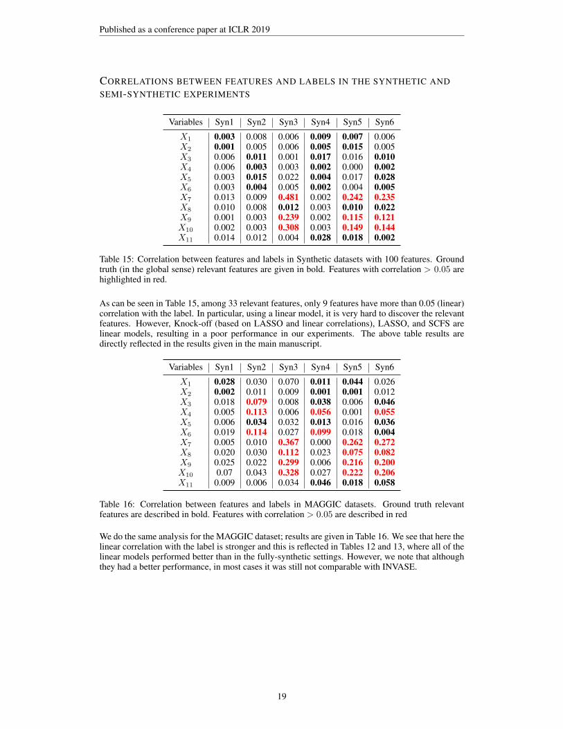
CORRELATIONS BETWEEN FEATURES AND LABELS IN THE SYNTHETIC ANDSEMI-SYNTHETIC EXPERIMENTS

Variables Syn1 Syn2 Syn3 Syn4 Syn5 Syn6

X1 0.003 0.008 0.006 0.009 0.007 0.006X2 0.001 0.005 0.006 0.005 0.015 0.005X3 0.006 0.011 0.001 0.017 0.016 0.010X4 0.006 0.003 0.003 0.002 0.000 0.002X5 0.003 0.015 0.022 0.004 0.017 0.028X6 0.003 0.004 0.005 0.002 0.004 0.005X7 0.013 0.009 0.481 0.002 0.242 0.235X8 0.010 0.008 0.012 0.003 0.010 0.022X9 0.001 0.003 0.239 0.002 0.115 0.121X10 0.002 0.003 0.308 0.003 0.149 0.144X11 0.014 0.012 0.004 0.028 0.018 0.002

Table 15: Correlation between features and labels in Synthetic datasets with 100 features. Groundtruth (in the global sense) relevant features are given in bold. Features with correlation > 0.05 arehighlighted in red.

As can be seen in Table 15, among 33 relevant features, only 9 features have more than 0.05 (linear)correlation with the label. In particular, using a linear model, it is very hard to discover the relevantfeatures. However, Knock-off (based on LASSO and linear correlations), LASSO, and SCFS arelinear models, resulting in a poor performance in our experiments. The above table results aredirectly reflected in the results given in the main manuscript.

Variables Syn1 Syn2 Syn3 Syn4 Syn5 Syn6

X1 0.028 0.030 0.070 0.011 0.044 0.026X2 0.002 0.011 0.009 0.001 0.001 0.012X3 0.018 0.079 0.008 0.038 0.006 0.046X4 0.005 0.113 0.006 0.056 0.001 0.055X5 0.006 0.034 0.032 0.013 0.016 0.036X6 0.019 0.114 0.027 0.099 0.018 0.004X7 0.005 0.010 0.367 0.000 0.262 0.272X8 0.020 0.030 0.112 0.023 0.075 0.082X9 0.025 0.022 0.299 0.006 0.216 0.200X10 0.07 0.043 0.328 0.027 0.222 0.206X11 0.009 0.006 0.034 0.046 0.018 0.058

Table 16: Correlation between features and labels in MAGGIC datasets. Ground truth relevantfeatures are described in bold. Features with correlation > 0.05 are described in red

We do the same analysis for the MAGGIC dataset; results are given in Table 16. We see that here thelinear correlation with the label is stronger and this is reflected in Tables 12 and 13, where all of thelinear models performed better than in the fully-synthetic settings. However, we note that althoughthey had a better performance, in most cases it was still not comparable with INVASE.

19


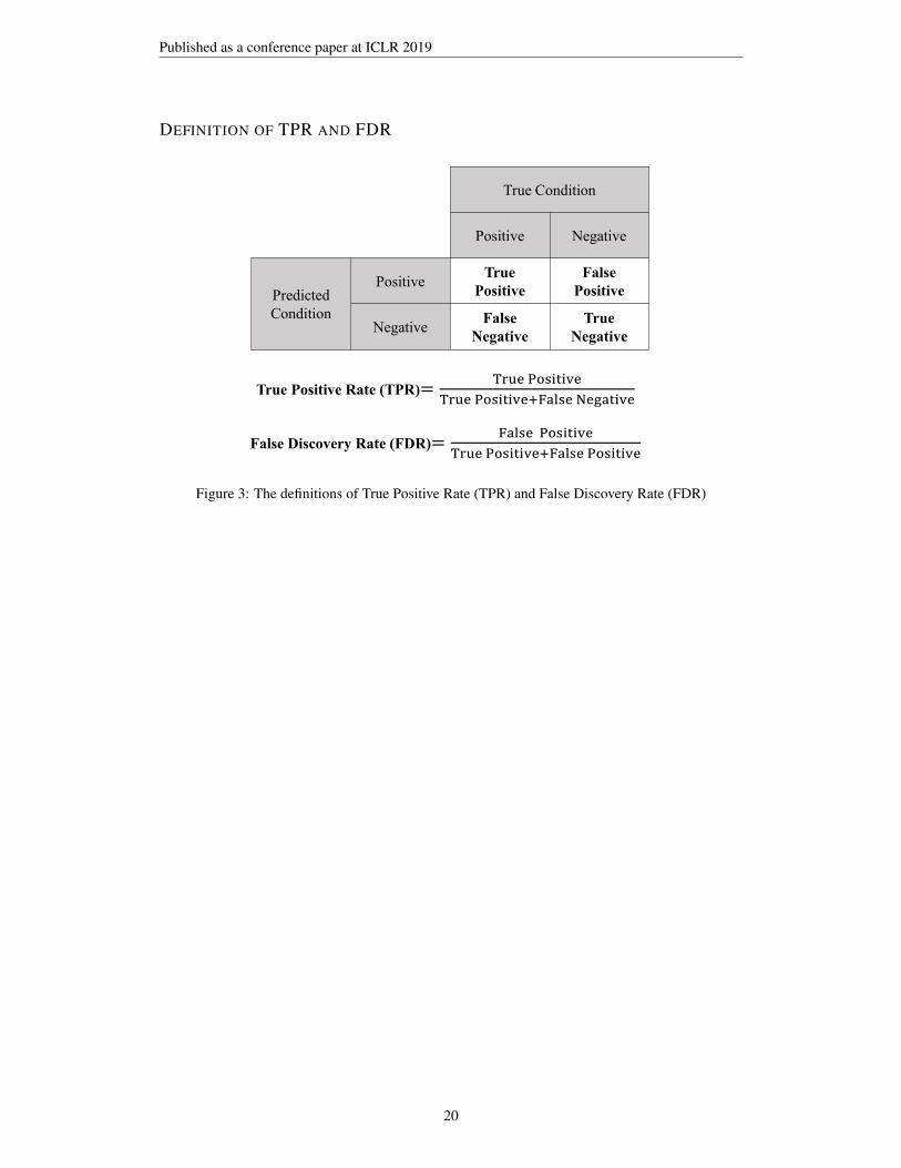
DEFINITION OF TPR AND FDR

True Condition

Positive Negative

Predicted Condition

PositiveTrue

PositiveFalse

Positive

NegativeFalse

NegativeTrue

Negative

True Positive Rate (TPR)=

False Discovery Rate (FDR)=

Figure 3: The definitions of True Positive Rate (TPR) and False Discovery Rate (FDR)

20


COMPUTER VISION

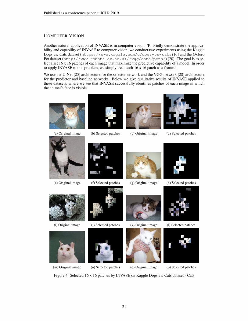
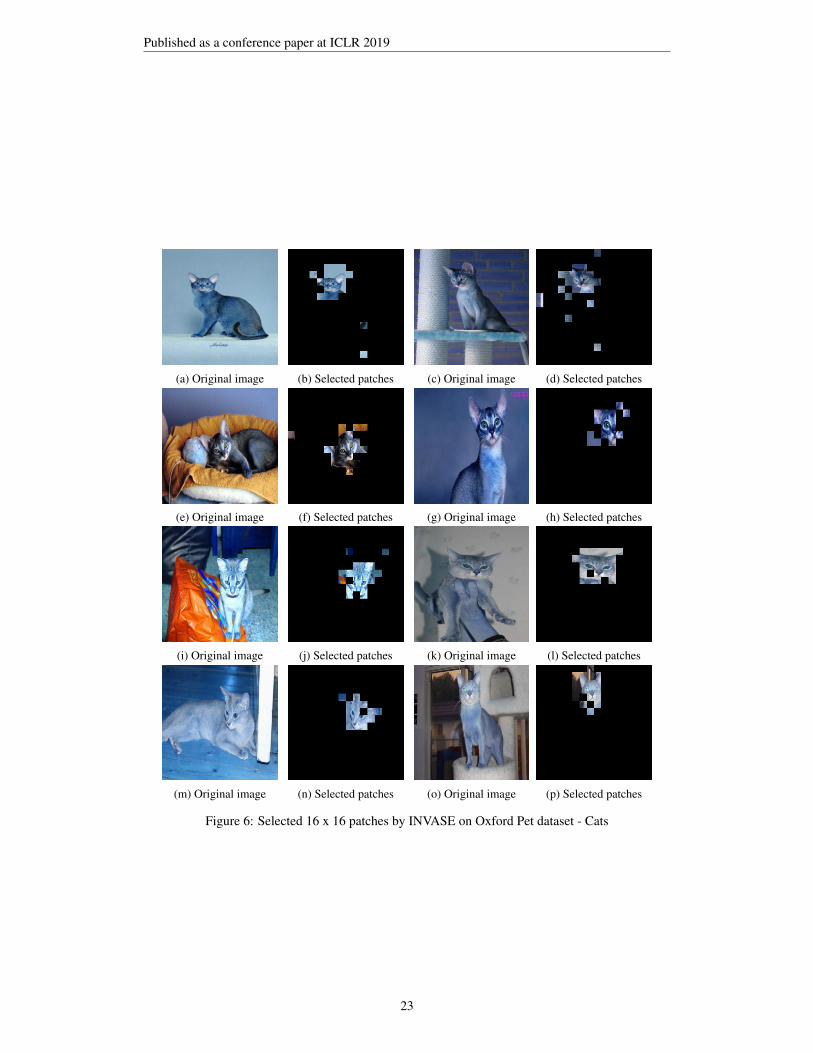
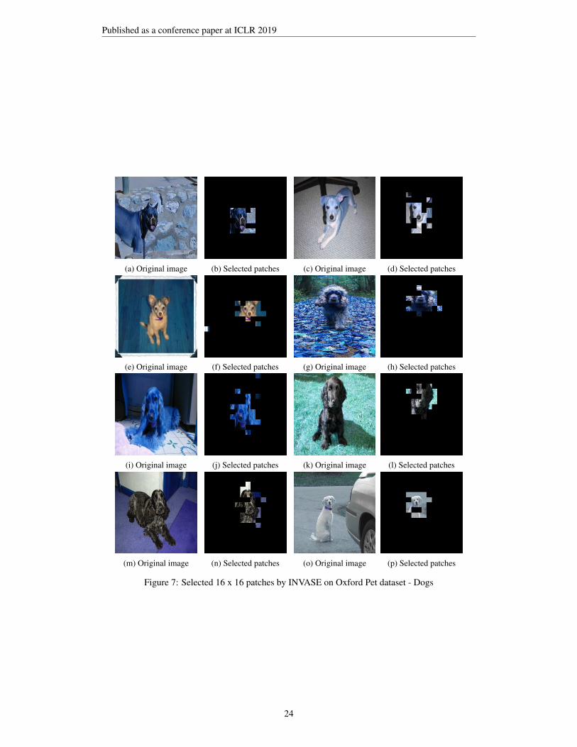
Another natural application of INVASE is in computer vision. To briefly demonstrate the applica-bility and capability of INVASE to computer vision, we conduct two experiments using the KaggleDogs vs. Cats dataset (https://www.kaggle.com/c/dogs-vs-cats) [6] and the OxfordPet dataset (http://www.robots.ox.ac.uk/˜vgg/data/pets/) [20]. The goal is to se-lect a set 16 x 16 patches of each image that maximize the predictive capability of a model. In orderto apply INVASE to this problem, we simply treat each 16 x 16 patch as a feature.

We use the U-Net [25] architecture for the selector network and the VGG network [28] architecturefor the predictor and baseline networks. Below we give qualitative results of INVASE applied tothese datasets, where we see that INVASE successfully identifies patches of each image in whichthe animal’s face is visible.

(a) Original image (b) Selected patches (c) Original image (d) Selected patches

(e) Original image (f) Selected patches (g) Original image (h) Selected patches

(i) Original image (j) Selected patches (k) Original image (l) Selected patches

(m) Original image (n) Selected patches (o) Original image (p) Selected patches

Figure 4: Selected 16 x 16 patches by INVASE on Kaggle Dogs vs. Cats dataset - Cats

21

https://www.kaggle.com/c/dogs-vs-cats

http://www.robots.ox.ac.uk/~vgg/data/pets/






Figure 5: Selected 16 x 16 patches by INVASE on Kaggle Dogs vs. Cats dataset - Dogs

22






Figure 6: Selected 16 x 16 patches by INVASE on Oxford Pet dataset - Cats

23






Figure 7: Selected 16 x 16 patches by INVASE on Oxford Pet dataset - Dogs

24

Documents

INVASE: I WISE VARIABLE SELECTION US ING N