Invariant of curves under Möbius group in 3-dimensional …dean.pku.edu.cn/bksky/2000xzjjlwjlk/5.pdf · group in 3-dimensional space ... We define a complete Möbius invariant

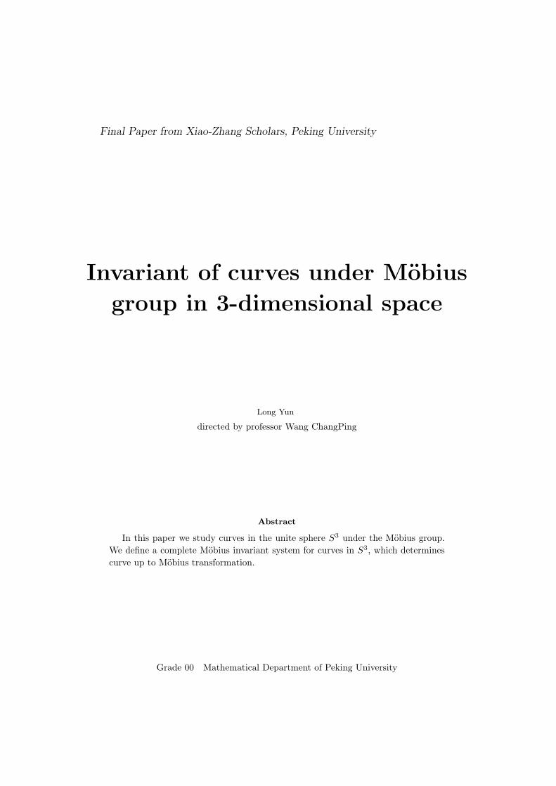
Final Paper from Xiao-Zhang Scholars, Peking University

Invariant of curves under Mobius

group in 3-dimensional space

Long Yun

directed by professor Wang ChangPing

Abstract

In this paper we study curves in the unite sphere S3 under the Mobius group.We define a complete Mobius invariant system for curves in S3, which determinescurve up to Mobius transformation.

Grade 00 Mathematical Department of Peking University

Papers of Xiao-Zhang Scholars, Peking University(2003)

1 Introduction to Mobius Geometry

Each type of geometry is defined by a group, and the researches on this geometry are tofind the invariant of figures under that transformation group.

Ordinary geometry is based on discussions of the length and angle which are invariant underisometry group in Rn space. If we instead isometry group with a new group—Mobius group,the following geometry will turn to a new kind. That is Mobius geometry which we mainlydiscuss in this article.

1.1 Two models of Mobius geometry

There’re two models for Mobius geometry—the unit n-sphere Sn lying in Euclidean (n+1)-space and the n-flat Rn ∪ {∞} we denoted Πn. We’ll define inversion in both of the models.

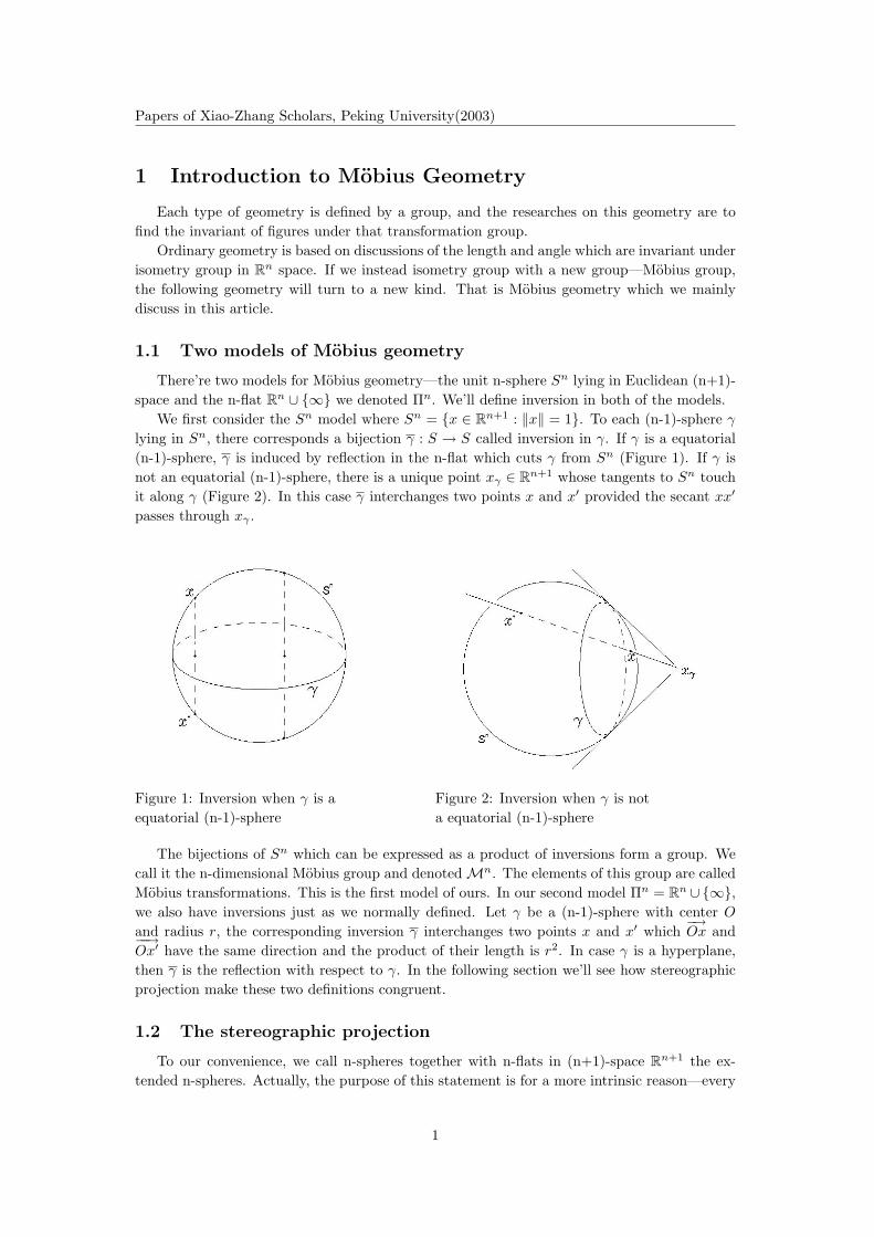
We first consider the Sn model where Sn = {x ∈ Rn+1 : ‖x‖ = 1}. To each (n-1)-sphere γ

lying in Sn, there corresponds a bijection γ : S → S called inversion in γ. If γ is a equatorial(n-1)-sphere, γ is induced by reflection in the n-flat which cuts γ from Sn (Figure 1). If γ isnot an equatorial (n-1)-sphere, there is a unique point xγ ∈ Rn+1 whose tangents to Sn touchit along γ (Figure 2). In this case γ interchanges two points x and x′ provided the secant xx′

passes through xγ .

Figure 1: Inversion when γ is aequatorial (n-1)-sphere

Figure 2: Inversion when γ is nota equatorial (n-1)-sphere

The bijections of Sn which can be expressed as a product of inversions form a group. Wecall it the n-dimensional Mobius group and denoted Mn. The elements of this group are calledMobius transformations. This is the first model of ours. In our second model Πn = Rn ∪{∞},we also have inversions just as we normally defined. Let γ be a (n-1)-sphere with center O

and radius r, the corresponding inversion γ interchanges two points x and x′ which−→Ox and−−→

Ox′ have the same direction and the product of their length is r2. In case γ is a hyperplane,then γ is the reflection with respect to γ. In the following section we’ll see how stereographicprojection make these two definitions congruent.

1.2 The stereographic projection

To our convenience, we call n-spheres together with n-flats in (n+1)-space Rn+1 the ex-tended n-spheres. Actually, the purpose of this statement is for a more intrinsic reason—every

1


two extended n-spheres can transfer to each-other under a Mobius group. That means n-spheresand n-flats share the same Mobius geometrical properties. They’re alike to some extent andshould have a common name.

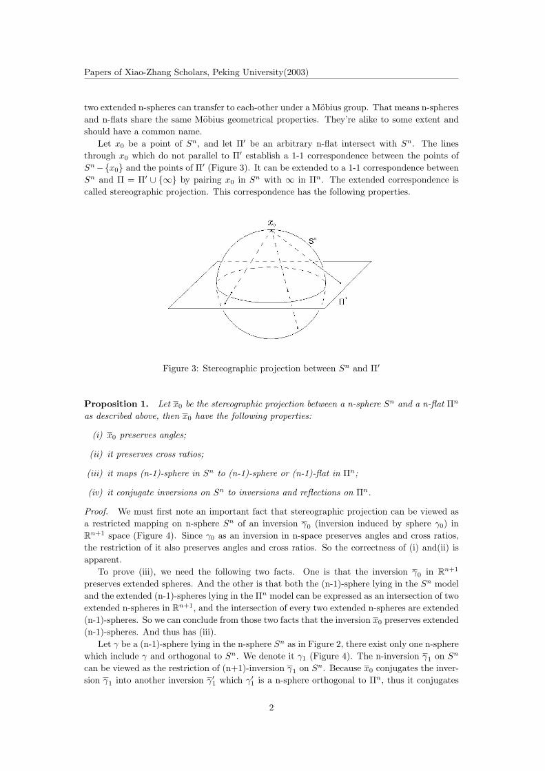
Let x0 be a point of Sn, and let Π′ be an arbitrary n-flat intersect with Sn. The linesthrough x0 which do not parallel to Π′ establish a 1-1 correspondence between the points ofSn−{x0} and the points of Π′ (Figure 3). It can be extended to a 1-1 correspondence betweenSn and Π = Π′ ∪ {∞} by pairing x0 in Sn with ∞ in Πn. The extended correspondence iscalled stereographic projection. This correspondence has the following properties.

Figure 3: Stereographic projection between Sn and Π′

Proposition 1. Let x0 be the stereographic projection between a n-sphere Sn and a n-flat Πn

as described above, then x0 have the following properties:

(i) x0 preserves angles;

(ii) it preserves cross ratios;

(iii) it maps (n-1)-sphere in Sn to (n-1)-sphere or (n-1)-flat in Πn;

(iv) it conjugate inversions on Sn to inversions and reflections on Πn.

Proof. We must first note an important fact that stereographic projection can be viewed asa restricted mapping on n-sphere Sn of an inversion γ0 (inversion induced by sphere γ0) inRn+1 space (Figure 4). Since γ0 as an inversion in n-space preserves angles and cross ratios,the restriction of it also preserves angles and cross ratios. So the correctness of (i) and(ii) isapparent.

To prove (iii), we need the following two facts. One is that the inversion γ0 in Rn+1

preserves extended spheres. And the other is that both the (n-1)-sphere lying in the Sn modeland the extended (n-1)-spheres lying in the Πn model can be expressed as an intersection of twoextended n-spheres in Rn+1, and the intersection of every two extended n-spheres are extended(n-1)-spheres. So we can conclude from those two facts that the inversion x0 preserves extended(n-1)-spheres. And thus has (iii).

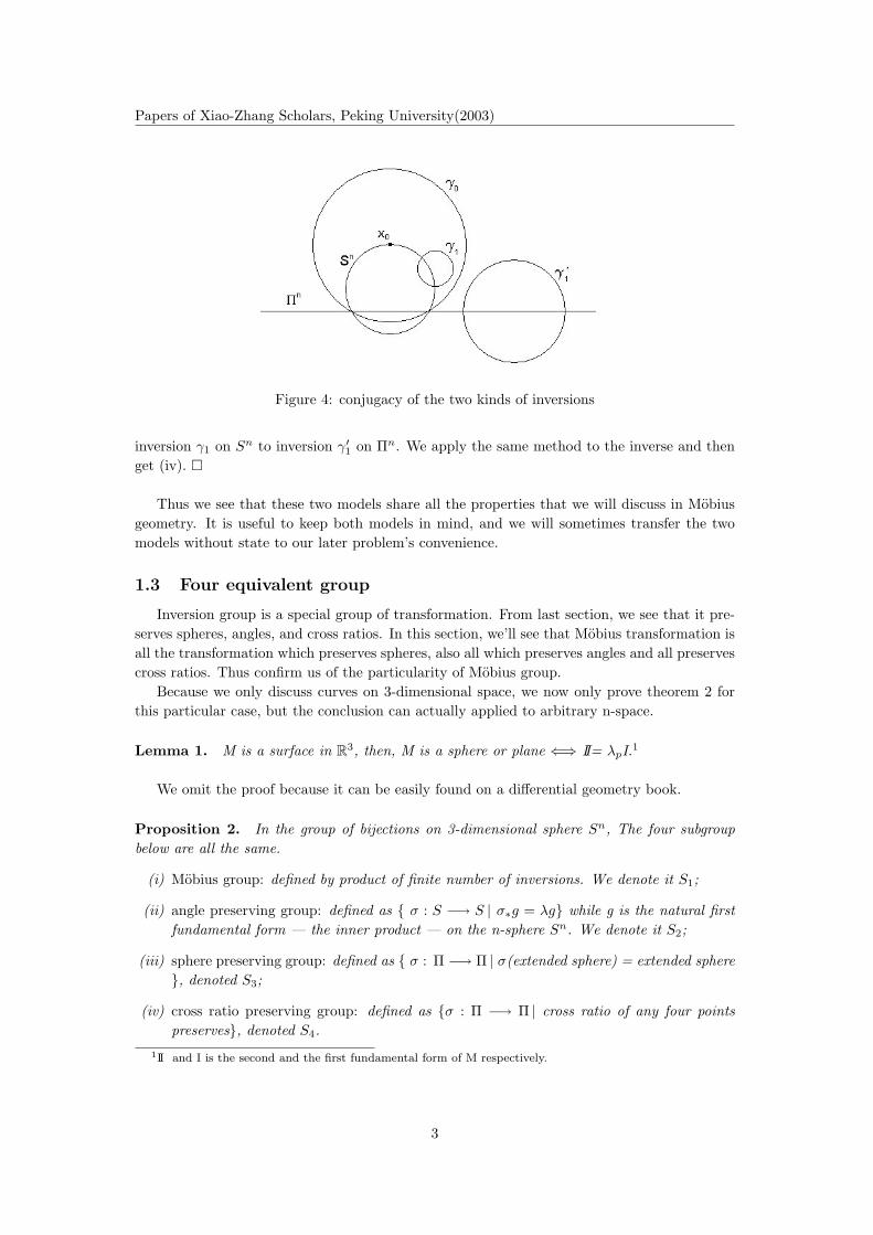
Let γ be a (n-1)-sphere lying in the n-sphere Sn as in Figure 2, there exist only one n-spherewhich include γ and orthogonal to Sn. We denote it γ1 (Figure 4). The n-inversion γ1 on Sn

can be viewed as the restriction of (n+1)-inversion γ1 on Sn. Because x0 conjugates the inver-sion γ1 into another inversion γ′1 which γ′1 is a n-sphere orthogonal to Πn, thus it conjugates

2


Figure 4: conjugacy of the two kinds of inversions

inversion γ1 on Sn to inversion γ′1 on Πn. We apply the same method to the inverse and thenget (iv). �

Thus we see that these two models share all the properties that we will discuss in Mobiusgeometry. It is useful to keep both models in mind, and we will sometimes transfer the twomodels without state to our later problem’s convenience.

1.3 Four equivalent group

Inversion group is a special group of transformation. From last section, we see that it pre-serves spheres, angles, and cross ratios. In this section, we’ll see that Mobius transformation isall the transformation which preserves spheres, also all which preserves angles and all preservescross ratios. Thus confirm us of the particularity of Mobius group.

Because we only discuss curves on 3-dimensional space, we now only prove theorem 2 forthis particular case, but the conclusion can actually applied to arbitrary n-space.

Lemma 1. M is a surface in R3, then, M is a sphere or plane ⇐⇒ II= λpI.1

We omit the proof because it can be easily found on a differential geometry book.

Proposition 2. In the group of bijections on 3-dimensional sphere Sn, The four subgroupbelow are all the same.

(i) Mobius group: defined by product of finite number of inversions. We denote it S1;

(ii) angle preserving group: defined as { σ : S −→ S | σ∗g = λg} while g is the natural firstfundamental form — the inner product — on the n-sphere Sn. We denote it S2;

(iii) sphere preserving group: defined as { σ : Π −→ Π | σ(extended sphere) = extended sphere}, denoted S3;

(iv) cross ratio preserving group: defined as {σ : Π −→ Π | cross ratio of any four pointspreserves}, denoted S4.

1II and I is the second and the first fundamental form of M respectively.

3


Proof. (i)−→(ii): result directly from Theorem 1.

(ii)−→(iii): From the discussions in reference [3], we know that an angle preserving trans-formation preserves the umbilics surfaces. Also from this reference, we know that the extendedspheres are all surfaces which all points on it are umbilics. So the image of an extended sphereunder an angle preserving transformation is a surface with all points are umbilics, and thus aextended sphere too.

(iii)−→(iv): we prove that a differential transformation f which preserves extended spherewill also preserve cross ratio.

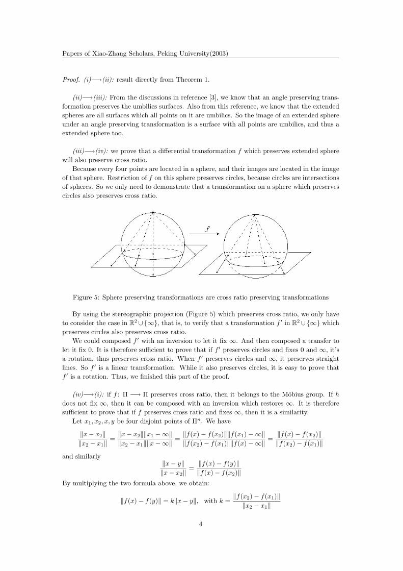
Because every four points are located in a sphere, and their images are located in the imageof that sphere. Restriction of f on this sphere preserves circles, because circles are intersectionsof spheres. So we only need to demonstrate that a transformation on a sphere which preservescircles also preserves cross ratio.

Figure 5: Sphere preserving transformations are cross ratio preserving transformations

By using the stereographic projection (Figure 5) which preserves cross ratio, we only haveto consider the case in R2 ∪{∞}, that is, to verify that a transformation f ′ in R2 ∪{∞} whichpreserves circles also preserves cross ratio.

We could composed f ′ with an inversion to let it fix ∞. And then composed a transfer tolet it fix 0. It is therefore sufficient to prove that if f ′ preserves circles and fixes 0 and ∞, it’sa rotation, thus preserves cross ratio. When f ′ preserves circles and ∞, it preserves straightlines. So f ′ is a linear transformation. While it also preserves circles, it is easy to prove thatf ′ is a rotation. Thus, we finished this part of the proof.

(iv)−→(i): if f : Π −→ Π preserves cross ratio, then it belongs to the Mobius group. If h

does not fix ∞, then it can be composed with an inversion which restores ∞. It is thereforesufficient to prove that if f preserves cross ratio and fixes ∞, then it is a similarity.

Let x1, x2, x, y be four disjoint points of Πn. We have

‖x− x2‖‖x2 − x1‖

=‖x− x2‖‖x1 −∞‖‖x2 − x1‖‖x−∞‖

=‖f(x)− f(x2)‖‖f(x1)−∞‖‖f(x2)− f(x1)‖‖f(x)−∞‖

=‖f(x)− f(x2)‖‖f(x2)− f(x1)‖

and similarly‖x− y‖‖x− x2‖

=‖f(x)− f(y)‖‖f(x)− f(x2)‖

By multiplying the two formula above, we obtain:

‖f(x)− f(y)‖ = k‖x− y‖, with k =‖f(x2)− f(x1)‖‖x2 − x1‖

4


it implies that f is a similarity and therefore a Mobius transformation. �

1.4 Isomorphic to the linear group L↑n+2

Recall our dealing with the curves under isometry group in R3, we get the invariant fromthe inner product which is an invariant under isometry group. To deal with our new nonlineargroup — the Mobius group, we want to search a new isomorph which could then apply thesame method. A solution is to map the Mobius group to a bilinear form preserving linear groupL↑n+2. So we could get our invariant in terms of the bilinear form. An elaborate description ofthis correspondence can be found in reference [1]. We only state the conclusions here and omitthe proofs.

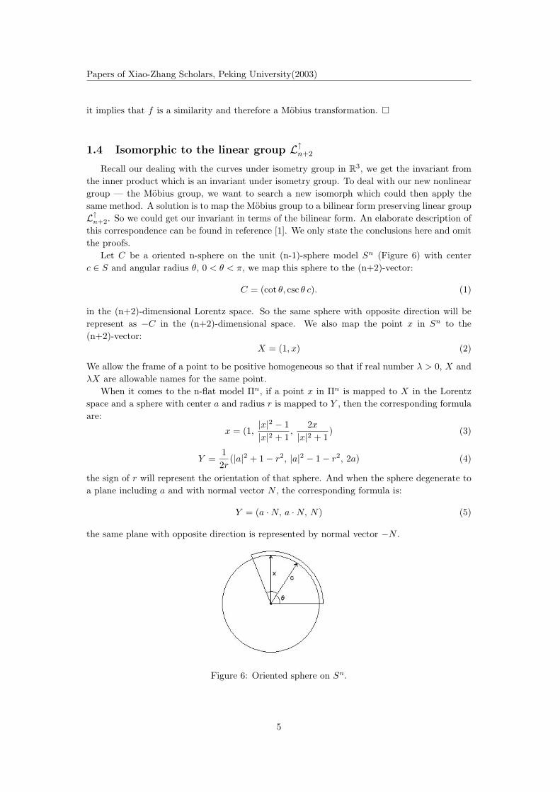
Let C be a oriented n-sphere on the unit (n-1)-sphere model Sn (Figure 6) with centerc ∈ S and angular radius θ, 0 < θ < π, we map this sphere to the (n+2)-vector:

C = (cot θ, csc θ c). (1)

in the (n+2)-dimensional Lorentz space. So the same sphere with opposite direction will berepresent as −C in the (n+2)-dimensional space. We also map the point x in Sn to the(n+2)-vector:

X = (1, x) (2)

We allow the frame of a point to be positive homogeneous so that if real number λ > 0, X andλX are allowable names for the same point.

When it comes to the n-flat model Πn, if a point x in Πn is mapped to X in the Lorentzspace and a sphere with center a and radius r is mapped to Y , then the corresponding formulaare:

x = (1,|x|2 − 1|x|2 + 1

,2x

|x|2 + 1) (3)

Y =12r

(|a|2 + 1− r2, |a|2 − 1− r2, 2a) (4)

the sign of r will represent the orientation of that sphere. And when the sphere degenerate toa plane including a and with normal vector N , the corresponding formula is:

Y = (a ·N, a ·N, N) (5)

the same plane with opposite direction is represented by normal vector −N .

Figure 6: Oriented sphere on Sn.

5


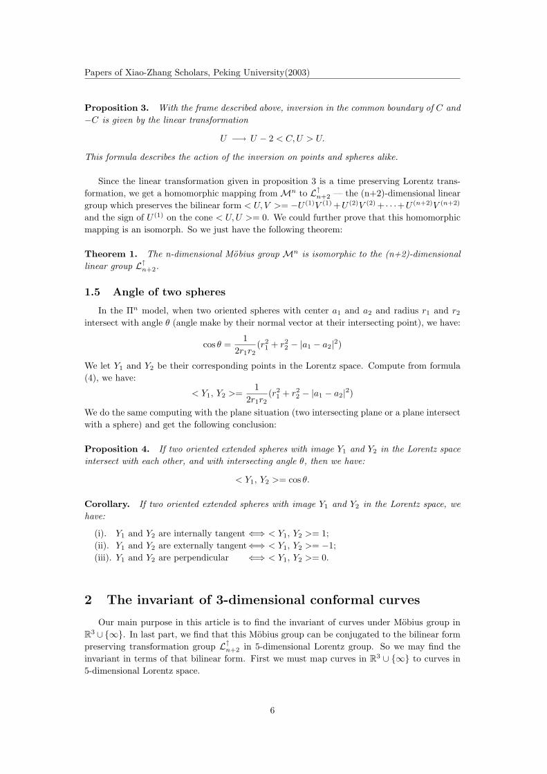
Proposition 3. With the frame described above, inversion in the common boundary of C and−C is given by the linear transformation

U −→ U − 2 < C, U > U.

This formula describes the action of the inversion on points and spheres alike.

Since the linear transformation given in proposition 3 is a time preserving Lorentz trans-formation, we get a homomorphic mapping from Mn to L↑n+2 — the (n+2)-dimensional lineargroup which preserves the bilinear form < U, V >= −U (1)V (1) +U (2)V (2) + · · ·+U (n+2)V (n+2)

and the sign of U (1) on the cone < U, U >= 0. We could further prove that this homomorphicmapping is an isomorph. So we just have the following theorem:

Theorem 1. The n-dimensional Mobius group Mn is isomorphic to the (n+2)-dimensionallinear group L↑n+2.

1.5 Angle of two spheres

In the Πn model, when two oriented spheres with center a1 and a2 and radius r1 and r2

intersect with angle θ (angle make by their normal vector at their intersecting point), we have:

cos θ =1

2r1r2(r2

1 + r22 − |a1 − a2|2)

We let Y1 and Y2 be their corresponding points in the Lorentz space. Compute from formula(4), we have:

< Y1, Y2 >=1

2r1r2(r2

1 + r22 − |a1 − a2|2)

We do the same computing with the plane situation (two intersecting plane or a plane intersectwith a sphere) and get the following conclusion:

Proposition 4. If two oriented extended spheres with image Y1 and Y2 in the Lorentz spaceintersect with each other, and with intersecting angle θ, then we have:

< Y1, Y2 >= cos θ.

Corollary. If two oriented extended spheres with image Y1 and Y2 in the Lorentz space, wehave:

(i). Y1 and Y2 are internally tangent ⇐⇒ < Y1, Y2 >= 1;(ii). Y1 and Y2 are externally tangent⇐⇒ < Y1, Y2 >= −1;(iii). Y1 and Y2 are perpendicular ⇐⇒ < Y1, Y2 >= 0.

2 The invariant of 3-dimensional conformal curves

Our main purpose in this article is to find the invariant of curves under Mobius group inR3 ∪ {∞}. In last part, we find that this Mobius group can be conjugated to the bilinear formpreserving transformation group L↑n+2 in 5-dimensional Lorentz group. So we may find theinvariant in terms of that bilinear form. First we must map curves in R3 ∪ {∞} to curves in5-dimensional Lorentz space.

6


2.1 Osculating sphere and it’s conjugacy of curves in 5-dimensional

Lorentz space

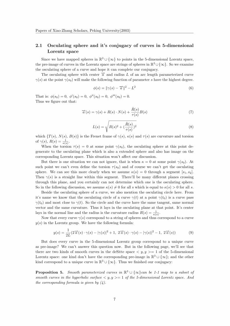
Since we have mapped spheres in R3 ∪ {∞} to points in the 5-dimensional Lorentz space,the pre-image of curves in the Lorentz space are strings of spheres in R3∪{∞}. So we examinethe osculating sphere of a curve and hope it can complete our conjugacy.

The osculating sphere with center −→a and radius L of an arc length parameterized curveγ(s) at the point γ(s0) will make the following function of parameter s have the highest degree.

φ(s) = ‖γ(s)−−→a ‖2 − L2 (6)

That is: φ(s0) = 0, φ′(s0) = 0, φ′′(s0) = 0, φ′′′(s0) = 0.

Thus we figure out that:

−→a (s) = γ(s) + R(s) ·N(s) +R(s)τ(s)

B(s) (7)

L(s) =

√R(s)2 + (

R(s)τ(s)

)2 (8)

which {T (s), N(s), B(s)} is the Frenet frame of γ(s), κ(s) and τ(s) are curvature and torsionof γ(s), R(s) = 1

κ(s) .When the torsion τ(s) = 0 at some point γ(s0), the osculating sphere at this point de-

generate to the osculating plane which is also a extended sphere and also has image on thecorresponding Lorentz space. This situation won’t affect our discussion.

But there is one situation we can not ignore, that is when κ = 0 at some point γ(s0). Atsuch point we can’t even define the torsion τ(s0) and of course we can’t get the osculatingsphere. We can see this more clearly when we assume κ(s) = 0 through a segment [s1, s2].Then γ(s) is a straight line within this segment. There’ll be many different planes crossingthrough this plane, and you certainly can not determine which one is the osculating sphere.So in the following discussion, we assume κ(s) 6= 0 for all s which is equal to κ(s) > 0 for all s.

Beside the osculating sphere of a curve, we also mention the osculating circle here. Fromit’s name we know that the osculating circle of a curve γ(t) at a point γ(t0) is a curve passγ(t0) and most close to γ(t). So the circle and the curve have the same tangent, same normalvector and the same curvature. Thus it lays in the osculating plane at that point. It’s centerlays in the normal line and the radius is the curvature radius R(s) = 1

κ(s) .Now that every curve γ(s) correspond to a string of spheres and thus correspond to a curve

y(s) in the Lorentz group. We have the following formula:

y(s) =1

2L(2−→a (s) · γ(s)− |γ(s)|2 + 1, 2−→a (s) · γ(s)− |γ(s)|2 − 1, 2−→a (s)) (9)

But does every curve in the 5-dimensional Lorentz group correspond to a unique curveas pre-image? We can’t answer this question now. But in the following page, we’ll see thatthere are two kinds of smooth curves in the deSitte space < y, y >= 1 of the 5-dimensionalLorentz space: one kind don’t have the corresponding pre-image in R3 ∪ {∞}; and the otherkind correspond to a unique curve in R3 ∪ {∞}. Thus we finished our conjugacy:

Proposition 5. Smooth parameterized curves in R3 ∪ {∞}can be 1-1 map to a subset ofsmooth curves in the hyperbolic surface < y, y >= 1 of the 5-dimensional Lorentz space. Andthe corresponding formula is given by (4).

7


We have another correspondence which is also useful in our following discussion. Since everypoint in R3 ∪ {∞} also correspond to a point on the cone < x, x >= 0 in the Lorentz space,every curve γ(s) in R3 ∪ {∞} correspond to a curve x(s) in the Lorentz space as following:

x(s) = (1,|γ(s)|2 − 1|γ(s)|2 + 1

,2γ(s)

|γ(s)|2 + 1) (10)

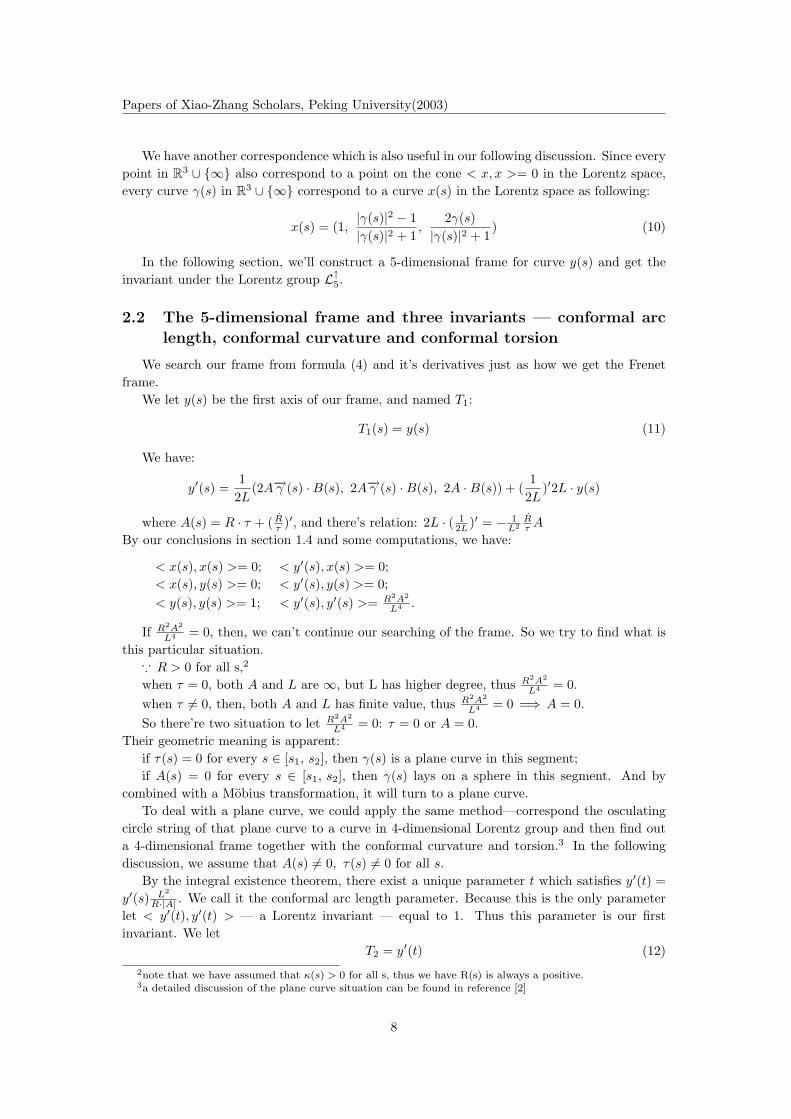
In the following section, we’ll construct a 5-dimensional frame for curve y(s) and get theinvariant under the Lorentz group L↑5.

2.2 The 5-dimensional frame and three invariants — conformal arc

length, conformal curvature and conformal torsion

We search our frame from formula (4) and it’s derivatives just as how we get the Frenetframe.

We let y(s) be the first axis of our frame, and named T1:

T1(s) = y(s) (11)

We have:

y′(s) =1

2L(2A−→γ (s) ·B(s), 2A−→γ (s) ·B(s), 2A ·B(s)) + (

12L

)′2L · y(s)

where A(s) = R · τ + ( Rτ )′, and there’s relation: 2L · ( 1

2L )′ = − 1L2

Rτ A

By our conclusions in section 1.4 and some computations, we have:

< x(s), x(s) >= 0; < y′(s), x(s) >= 0;< x(s), y(s) >= 0; < y′(s), y(s) >= 0;< y(s), y(s) >= 1; < y′(s), y′(s) >= R2A2

L4 .

If R2A2

L4 = 0, then, we can’t continue our searching of the frame. So we try to find what isthis particular situation.

∵ R > 0 for all s,2

when τ = 0, both A and L are ∞, but L has higher degree, thus R2A2

L4 = 0.when τ 6= 0, then, both A and L has finite value, thus R2A2

L4 = 0 =⇒ A = 0.So there’re two situation to let R2A2

L4 = 0: τ = 0 or A = 0.Their geometric meaning is apparent:

if τ(s) = 0 for every s ∈ [s1, s2], then γ(s) is a plane curve in this segment;if A(s) = 0 for every s ∈ [s1, s2], then γ(s) lays on a sphere in this segment. And by

combined with a Mobius transformation, it will turn to a plane curve.To deal with a plane curve, we could apply the same method—correspond the osculating

circle string of that plane curve to a curve in 4-dimensional Lorentz group and then find outa 4-dimensional frame together with the conformal curvature and torsion.3 In the followingdiscussion, we assume that A(s) 6= 0, τ(s) 6= 0 for all s.

By the integral existence theorem, there exist a unique parameter t which satisfies y′(t) =y′(s) L2

R·|A| . We call it the conformal arc length parameter. Because this is the only parameterlet < y′(t), y′(t) > — a Lorentz invariant — equal to 1. Thus this parameter is our firstinvariant. We let

T2 = y′(t) (12)2note that we have assumed that κ(s) > 0 for all s, thus we have R(s) is always a positive.3a detailed discussion of the plane curve situation can be found in reference [2]

8


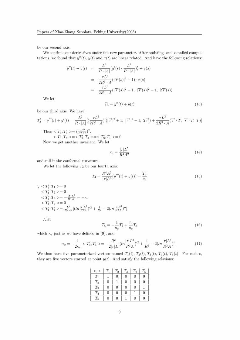
be our second axis.We continue our derivatives under this new parameter. After omitting some detailed compu-

tations, we found that y′′(t), y(t) and x(t) are linear related. And have the following relations:

y′′(t) + y(t) =L2

R · |A|(y′(s) · L2

R · |A|)′s + y(s)

=τL3

2R3 ·A(|−→r (s)|2 + 1) · x(s)

=τL3

2R3 ·A(|−→r (s)|2 + 1, |−→r (s)|2 − 1, 2−→r (s))

We letT3 = y′′(t) + y(t) (13)

be our third axis. We have:

T ′3 = y′′′(t) + y′(t) =

L2

R · |A|[(

τL3

2R3 ·A)′(|−→r |2 + 1, |−→r |2 − 1, 2−→r ) +

τL3

2R3 ·A(−→r · T, −→r · T, T )]

Thus < T ′3, T

′3 >= ( τL5

R4A2 )2.< T ′

3, T3 >=< T ′3, T2 >=< T ′

3, T1 >= 0Now we get another invariant. We let

κc =|τ |L5

R4A2(14)

and call it the conformal curvature.We let the following T4 be our fourth axis:

T4 =R4A2

|τ |L5(y′′′(t) + y(t)) =

T ′3

κc(15)

∵ < T ′4, T1 >= 0

< T ′4, T2 >= 0

< T ′4, T3 >= − |τ |L5

R4A2 = −κc

< T ′4, T4 >= 0

< T ′4, T

′4 >= L4

R2A2 [(ln |τ |L3

R3A )′2 + 1R2 − 2(ln |τ |L3

R3A )′′]

∴ letT5 = − 1

κcT ′

4 +τc

κcT3 (16)

which κc just as we have defined in (9), and

τc = − 12κc

< T ′4, T

′4 >= − R2

2|τ |L[(ln

|τ |L3

R3A)′2 +

1R2

− 2(ln|τ |L3

R3A)′′] (17)

We thus have five parameterized vectors named T1(t), T2(t), T3(t), T4(t), T5(t). For each s,they are five vectors started at point y(t). And satisfy the following relations:

<,> T1 T2 T3 T4 T5

T1 1 0 0 0 0T2 0 1 0 0 0T3 0 0 0 0 1T4 0 0 0 1 0T5 0 0 1 0 0

9


formula I

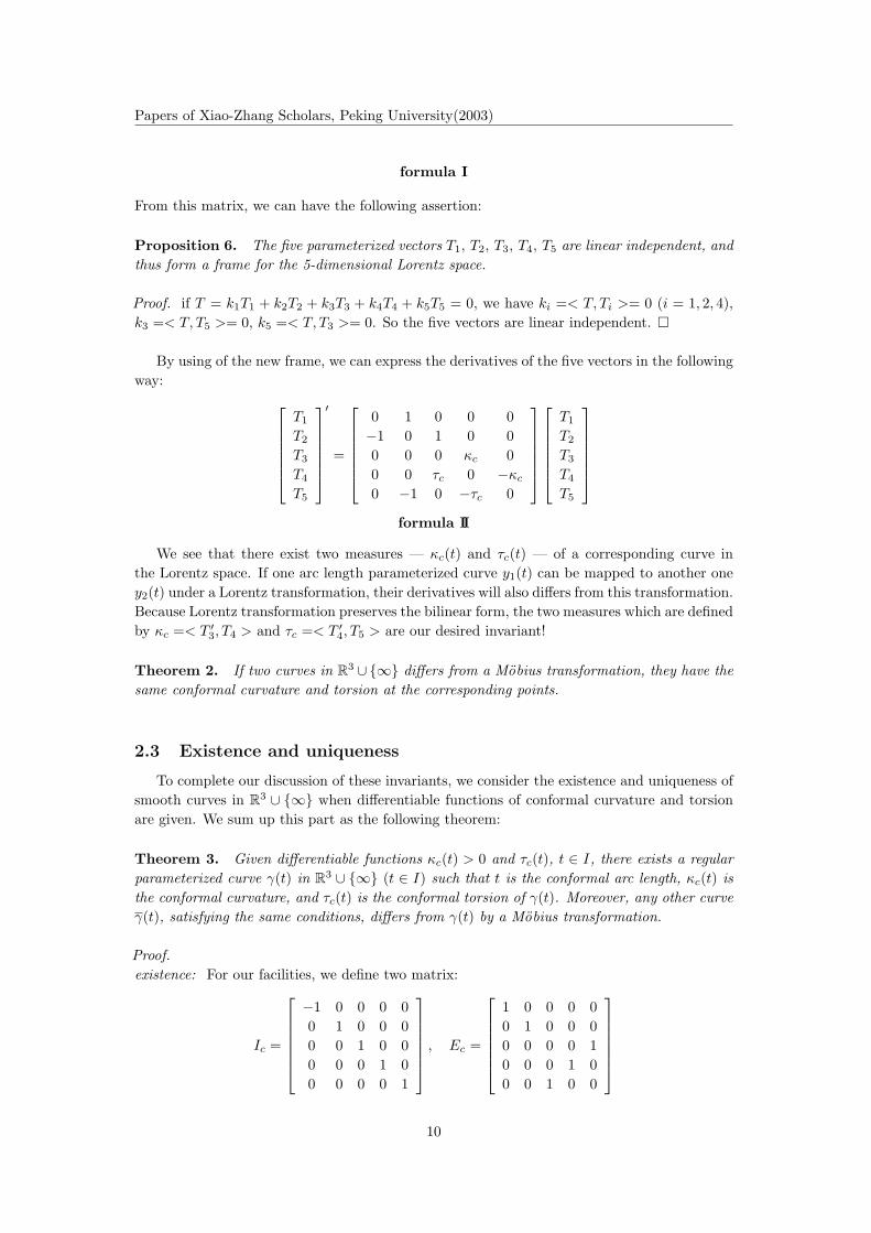
From this matrix, we can have the following assertion:

Proposition 6. The five parameterized vectors T1, T2, T3, T4, T5 are linear independent, andthus form a frame for the 5-dimensional Lorentz space.

Proof. if T = k1T1 + k2T2 + k3T3 + k4T4 + k5T5 = 0, we have ki =< T, Ti >= 0 (i = 1, 2, 4),k3 =< T, T5 >= 0, k5 =< T, T3 >= 0. So the five vectors are linear independent. �

By using of the new frame, we can express the derivatives of the five vectors in the followingway:

T1

T2

T3

T4

T5

′

=

0 1 0 0 0−1 0 1 0 00 0 0 κc 00 0 τc 0 −κc

0 −1 0 −τc 0

T1

T2

T3

T4

T5

formula II

We see that there exist two measures — κc(t) and τc(t) — of a corresponding curve inthe Lorentz space. If one arc length parameterized curve y1(t) can be mapped to another oney2(t) under a Lorentz transformation, their derivatives will also differs from this transformation.Because Lorentz transformation preserves the bilinear form, the two measures which are definedby κc =< T ′

3, T4 > and τc =< T ′4, T5 > are our desired invariant!

Theorem 2. If two curves in R3 ∪ {∞} differs from a Mobius transformation, they have thesame conformal curvature and torsion at the corresponding points.

2.3 Existence and uniqueness

To complete our discussion of these invariants, we consider the existence and uniqueness ofsmooth curves in R3 ∪ {∞} when differentiable functions of conformal curvature and torsionare given. We sum up this part as the following theorem:

Theorem 3. Given differentiable functions κc(t) > 0 and τc(t), t ∈ I, there exists a regularparameterized curve γ(t) in R3 ∪ {∞} (t ∈ I) such that t is the conformal arc length, κc(t) isthe conformal curvature, and τc(t) is the conformal torsion of γ(t). Moreover, any other curveγ(t), satisfying the same conditions, differs from γ(t) by a Mobius transformation.

Proof.existence: For our facilities, we define two matrix:

Ic =

−1 0 0 0 00 1 0 0 00 0 1 0 00 0 0 1 00 0 0 0 1

, Ec =

1 0 0 0 00 1 0 0 00 0 0 0 10 0 0 1 00 0 1 0 0

10


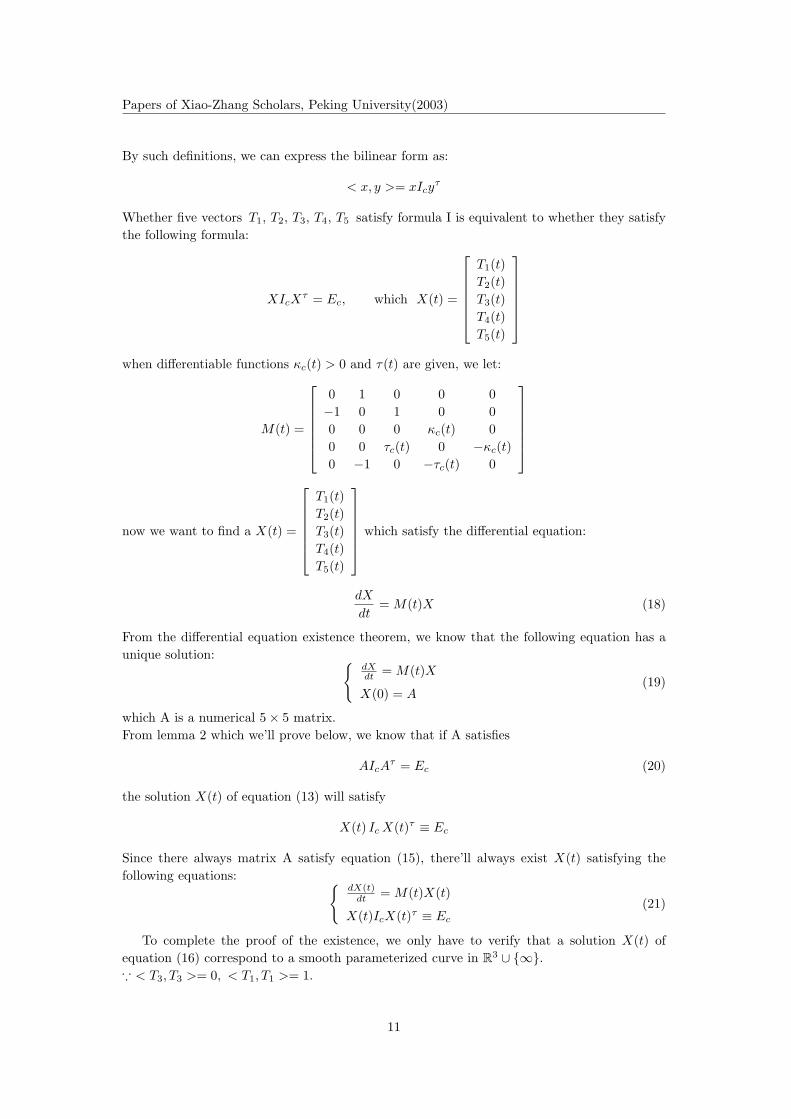
By such definitions, we can express the bilinear form as:

< x, y >= xIcyτ

Whether five vectors T1, T2, T3, T4, T5 satisfy formula I is equivalent to whether they satisfythe following formula:

XIcXτ = Ec, which X(t) =

T1(t)T2(t)T3(t)T4(t)T5(t)

when differentiable functions κc(t) > 0 and τ(t) are given, we let:

M(t) =

0 1 0 0 0−1 0 1 0 00 0 0 κc(t) 00 0 τc(t) 0 −κc(t)0 −1 0 −τc(t) 0

now we want to find a X(t) =


which satisfy the differential equation:

dX

dt= M(t)X (18)

From the differential equation existence theorem, we know that the following equation has aunique solution: {

dXdt = M(t)X

X(0) = A(19)

which A is a numerical 5× 5 matrix.From lemma 2 which we’ll prove below, we know that if A satisfies

AIcAτ = Ec (20)

the solution X(t) of equation (13) will satisfy

X(t) Ic X(t)τ ≡ Ec

Since there always matrix A satisfy equation (15), there’ll always exist X(t) satisfying thefollowing equations: {

dX(t)dt = M(t)X(t)

X(t)IcX(t)τ ≡ Ec

(21)

To complete the proof of the existence, we only have to verify that a solution X(t) ofequation (16) correspond to a smooth parameterized curve in R3 ∪ {∞}.∵ < T3, T3 >= 0, < T1, T1 >= 1.

11


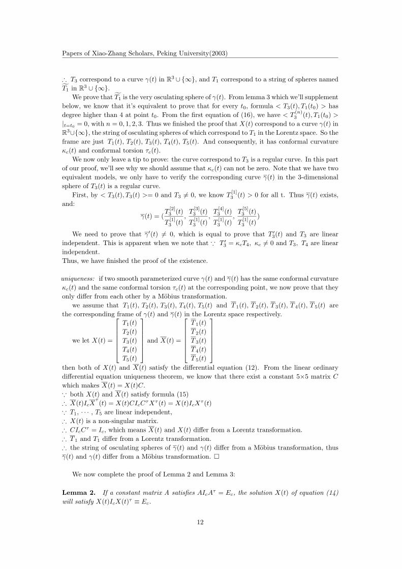
∴ T3 correspond to a curve γ(t) in R3 ∪ {∞}, and T1 correspond to a string of spheres namedT1 in R3 ∪ {∞}.

We prove that T1 is the very osculating sphere of γ(t). From lemma 3 which we’ll supplementbelow, we know that it’s equivalent to prove that for every t0, formula < T3(t), T1(t0) > hasdegree higher than 4 at point t0. From the first equation of (16), we have < T

(n)3 (t), T1(t0) >

|t=t0 = 0, with n = 0, 1, 2, 3. Thus we finished the proof that X(t) correspond to a curve γ(t) inR3∪{∞}, the string of osculating spheres of which correspond to T1 in the Lorentz space. So theframe are just T1(t), T2(t), T3(t), T4(t), T5(t). And consequently, it has conformal curvatureκc(t) and conformal torsion τc(t).

We now only leave a tip to prove: the curve correspond to T3 is a regular curve. In this partof our proof, we’ll see why we should assume that κc(t) can not be zero. Note that we have twoequivalent models, we only have to verify the corresponding curve γ(t) in the 3-dimensionalsphere of T3(t) is a regular curve.

First, by < T3(t), T3(t) >= 0 and T3 6= 0, we know T[1]3 (t) > 0 for all t. Thus γ(t) exists,

and:

γ(t) = (T

[2]3 (t)

T[1]3 (t)

,T

[3]3 (t)

T[1]3 (t)

,T

[4]3 (t)

T[1]3 (t)

,T

[5]3 (t)

T[1]3 (t)

)

We need to prove that γ′(t) 6= 0, which is equal to prove that T ′3(t) and T3 are linear

independent. This is apparent when we note that ∵ T ′3 = κcT4, κc 6= 0 and T3, T4 are linear

independent.Thus, we have finished the proof of the existence.

uniqueness: if two smooth parameterized curve γ(t) and γ(t) has the same conformal curvatureκc(t) and the same conformal torsion τc(t) at the corresponding point, we now prove that theyonly differ from each other by a Mobius transformation.

we assume that T1(t), T2(t), T3(t), T4(t), T5(t) and T 1(t), T 2(t), T 3(t), T 4(t), T 5(t) arethe corresponding frame of γ(t) and γ(t) in the Lorentz space respectively.

we let X(t) =


and X(t) =

T 1(t)T 2(t)T 3(t)T 4(t)T 5(t)

then both of X(t) and X(t) satisfy the differential equation (12). From the linear ordinarydifferential equation uniqueness theorem, we know that there exist a constant 5×5 matrix C

which makes X(t) = X(t)C.∵ both X(t) and X(t) satisfy formula (15)∴ X(t)IcX

τ(t) = X(t)CIcC

τXτ (t) = X(t)IcXτ (t)

∵ T1, · · · , T5 are linear independent,∴ X(t) is a non-singular matrix.∴ CIcC

τ = Ic, which means X(t) and X(t) differ from a Lorentz transformation.∴ T 1 and T1 differ from a Lorentz transformation.∴ the string of osculating spheres of γ(t) and γ(t) differ from a Mobius transformation, thusγ(t) and γ(t) differ from a Mobius transformation. �

We now complete the proof of Lemma 2 and Lemma 3:

Lemma 2. If a constant matrix A satisfies AIcAτ = Ec, the solution X(t) of equation (14)

will satisfy X(t)IcX(t)τ ≡ Ec.

12


Proof. let Y (t) = X(t)IcX(t)τ ;

then

{Y (0) = Ic

dYdt = dX

dt IcX(t)τ + X(t)Ic(dXdt )τ = M(t)Y (t) + Y (t)M(t)τ

From the differential equation existence theorem, the above equation of Y has a unique solu-tion. Since Y ≡ Ec is a solution, we have Y ≡ Ec. �

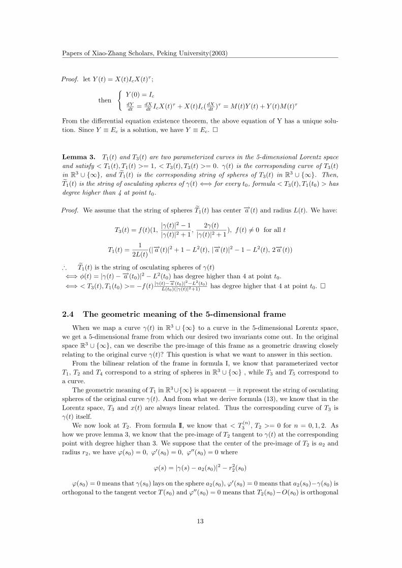
Lemma 3. T1(t) and T3(t) are two parameterized curves in the 5-dimensional Lorentz spaceand satisfy < T1(t), T1(t) >= 1, < T3(t), T3(t) >= 0. γ(t) is the corresponding curve of T3(t)in R3 ∪ {∞}, and T1(t) is the corresponding string of spheres of T3(t) in R3 ∪ {∞}. Then,T1(t) is the string of osculating spheres of γ(t) ⇐⇒ for every t0, formula < T3(t), T1(t0) > hasdegree higher than 4 at point t0.

Proof. We assume that the string of spheres T1(t) has center −→a (t) and radius L(t). We have:

T3(t) = f(t)(1,|γ(t)|2 − 1|γ(t)|2 + 1

,2γ(t)

|γ(t)|2 + 1), f(t) 6= 0 for all t

T1(t) =1

2L(t)(|−→a (t)|2 + 1− L2(t), |−→a (t)|2 − 1− L2(t), 2−→a (t))

∴ T1(t) is the string of osculating spheres of γ(t)⇐⇒ φ(t) = |γ(t)−−→a (t0)|2 − L2(t0) has degree higher than 4 at point t0.⇐⇒ < T3(t), T1(t0) >= −f(t) |γ(t)−−→a (t0)|2−L2(t0)

L(t0)(|γ(t)|2+1) has degree higher that 4 at point t0. �

2.4 The geometric meaning of the 5-dimensional frame

When we map a curve γ(t) in R3 ∪ {∞} to a curve in the 5-dimensional Lorentz space,we get a 5-dimensional frame from which our desired two invariants come out. In the originalspace R3 ∪ {∞}, can we describe the pre-image of this frame as a geometric drawing closelyrelating to the original curve γ(t)? This question is what we want to answer in this section.

From the bilinear relation of the frame in formula I, we know that parameterized vectorT1, T2 and T4 correspond to a string of spheres in R3 ∪ {∞} , while T3 and T5 correspond toa curve.

The geometric meaning of T1 in R3∪{∞} is apparent — it represent the string of osculatingspheres of the original curve γ(t). And from what we derive formula (13), we know that in theLorentz space, T3 and x(t) are always linear related. Thus the corresponding curve of T3 isγ(t) itself.

We now look at T2. From formula II, we know that < T(n)3 , T2 >= 0 for n = 0, 1, 2. As

how we prove lemma 3, we know that the pre-image of T2 tangent to γ(t) at the correspondingpoint with degree higher than 3. We suppose that the center of the pre-image of T2 is a2 andradius r2, we have ϕ(s0) = 0, ϕ′(s0) = 0, ϕ′′(s0) = 0 where

ϕ(s) = |γ(s)− a2(s0)|2 − r22(s0)

ϕ(s0) = 0 means that γ(s0) lays on the sphere a2(s0), ϕ′(s0) = 0 means that a2(s0)−γ(s0) isorthogonal to the tangent vector T (s0) and ϕ′′(s0) = 0 means that T2(s0)−O(s0) is orthogonal

13


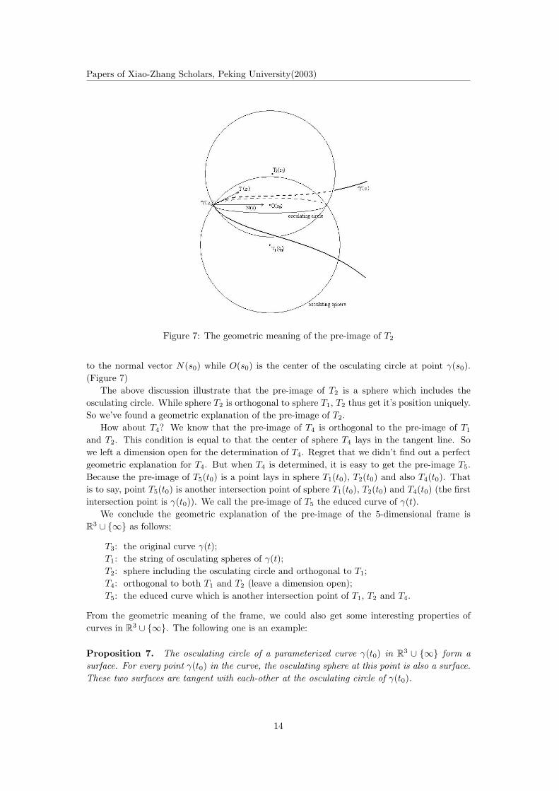
Figure 7: The geometric meaning of the pre-image of T2

to the normal vector N(s0) while O(s0) is the center of the osculating circle at point γ(s0).(Figure 7)

The above discussion illustrate that the pre-image of T2 is a sphere which includes theosculating circle. While sphere T2 is orthogonal to sphere T1, T2 thus get it’s position uniquely.So we’ve found a geometric explanation of the pre-image of T2.

How about T4? We know that the pre-image of T4 is orthogonal to the pre-image of T1

and T2. This condition is equal to that the center of sphere T4 lays in the tangent line. Sowe left a dimension open for the determination of T4. Regret that we didn’t find out a perfectgeometric explanation for T4. But when T4 is determined, it is easy to get the pre-image T5.Because the pre-image of T5(t0) is a point lays in sphere T1(t0), T2(t0) and also T4(t0). Thatis to say, point T5(t0) is another intersection point of sphere T1(t0), T2(t0) and T4(t0) (the firstintersection point is γ(t0)). We call the pre-image of T5 the educed curve of γ(t).

We conclude the geometric explanation of the pre-image of the 5-dimensional frame isR3 ∪ {∞} as follows:

T3: the original curve γ(t);T1: the string of osculating spheres of γ(t);T2: sphere including the osculating circle and orthogonal to T1;T4: orthogonal to both T1 and T2 (leave a dimension open);T5: the educed curve which is another intersection point of T1, T2 and T4.

From the geometric meaning of the frame, we could also get some interesting properties ofcurves in R3 ∪ {∞}. The following one is an example:

Proposition 7. The osculating circle of a parameterized curve γ(t0) in R3 ∪ {∞} form asurface. For every point γ(t0) in the curve, the osculating sphere at this point is also a surface.These two surfaces are tangent with each-other at the osculating circle of γ(t0).

14


Proof. We know that the osculating circle is the intersecting of the pre-image of T1 and T2.We assume a parameterized curve γ(t), for every t0, γ(t0) lies in the osculating circle of γ(t0).Then γ(t) always lays in the pre-image of T1(t) and T2(t). We denote the corresponding curveof γ(t) in Lorentz space as y(t). We have < y(t), T1(t) >≡ 0 and < y(t), T2(t) >≡ 0. Wederive from formula I and get < y′(t), T1(t) >≡ 0 which means γ(t) tangent with the osculatingsphere. From the randomness of the chosen of γ(t), we complete the proof. �

3 Examples of conformal curves

To get a more clear understanding of curves under Mobius geometry, we now look at somespecial curves and draw out some images.

One such kind of curves is those with constant conformal curvature and torsion. And nowwe begin our discussion of them.

3.1 curves with constant conformal curvature and torsion

We first examine the spirals which have constant common curvature and torsion. We knowfrom (9) and (12) that this kind of curves have constant conformal curvature and torsion. Theformula of spirals can be expressed as follows:

γ(s) =1√

a2 + r2(r cos s, rsins, as)

which s is the common arc length parameter.their common curvature κ and torsion τ are:

κ =r√

a2 + r2; τ = − a√

a2 + r2

From formula (9) and (12) we have: 4

κc =1

Rτ=

r

a; τc =

12τR

=r

2a

So we find that all the spirals are curves with constant conformal curvature and torsion andsatisfy κc = 2τc

To a more general situation, given any two constant κc and τc, we now try to find a regularcurve which has κc as its conformal curvature and τc as its conformal torsion. And all curveswith conformal curvature κc and conformal torsion τc are images of this curve under Mobiustransformations.

We start from the differential equation in formula II and try to get a solution. since we canget qualified curves directly from T3, we search the solution of T3 in formula II. We assume thatsome component of T3 has style as coshαx or cos βx, then from formula II, we have:

T3 coshαx cos βx

T4ακc

sinhαx − βκc

sinβx

T5 ( τc

κc− α2

κ2c) coshαx ( τc

κc+ β2

κ2c) cos βx

4computer directly from (9) and (12) is not a good method to get the conformal curvature and torsion. In

the practice, find the 5-dimensional frame and compute their bilinear form is a more favorable method. But

in this particular situation, when the common curvature and torsion are constant and thus have derivative 0,

using (9) and (12) is an easier way.

15


T2 −α( 2τc

κc− α2

κ2c) sinhαx β( 2τc

κc− β2

κ2c) sinβx

T1 [1 + α2( 2τc

κc− α2

κ2c)] coshαx [1 + β2( 2τc

κc− β2

κ2c)] cos βx

α and β satisfy:

(α2

κ2c

− 2τc

κc)(1 + α2) = 1 (22)

(β2

κ2c

+2τc

κc)(β2 − 1) = 1 (23)

the same applied when the style of some component of T3 is sinhαx or sin αx. Consider thenumber of solutions of equation (13) and (14), we have:

Case (i) : − 2τc

κc< 1, that is τc

κc> − 1

2

In this situation, equation (13) and (14) both have a unique solution.So the five fundamental solutions of T3 are:

coshαx, sinhαx, cos βx, sinβx, 1

α and β are positive root of (13) and (14) respectively, and we have α > 0, β > 1.Reversely, given two constant α > 0 and β > 1, we can get a unique pair of κc and τc from(13) and (14): {

k2c = (β2 − 1)(α2 + 1)

2κcτc = α2 − β2 + 1

Thus we correspond every (κc, τc) satisfying τc

κc> − 1

2 with pair (α, β) satisfying α > 0, β >

1. And we try to find a satisfying curve in R3 ∪ {∞} parameterized by α and β.If every components of T3 are linear combinations of the five fundamental solutions, it will

satisfy differential equation in formula II. We only has to determine the coefficient to makeT1 ∼ T5 satisfy formula I.∵< T3, T3 >= 0, we consider solution with style:

T3 = (b coshαx, b sinhαx, a cos βx, a sinβx, c)

x is the conformal arc length parameter.From lemma 2, we only have to prove that formula I satisfied when x = 0. When x = 0, wehave:

T3 : ( b 0 a 0 c )T4 : ( 0 b α

κc0 a β

κc0 )

T5 : ( b( τc

κc− α2

κ2c) 0 a( τc

κc+ β2

κ2c) 0 c τc

κc)

T2 : ( 0 bα( 2τc

κc− α2

κ2c) 0 aβ( 2τc

κc+ β2

κ2c) 0 )

T1 : ( b(α2

κ2c− 2τc

κc) 0 a(β2

κ2c

+ 2τc

κc) 0 c )

so formula I ⇐⇒

a2 − b2 = − κc

κc+2τc

b2α2 + a2β2 = κ2c

c2 = b2 − a2

⇐⇒

a2 = (β2−1)2(α2+1)

(α2+β2)β2

b2 = (β2−1)(α2+1)2

(α2+β2)α2

c2 = b2 − a2

We thus get T3, and then the corresponding curve γ(x) in R3 ∪ {∞} as follows:

γ(x) = eαx(a

bcos βx,

a

bsinβx,

√1− a2

b2)

16


with two parameter α > 0, β > 1, and ab = α

β

√β2−1α2+1

x is the conformal arc parameter.This is all qualified curves in case (i).

Case (ii): τc

κc< − 1

2

The five fundamental solutions of T3 are:

(cos β1x, sinβ1x, cos β2x, sinβ2x, 1)

β1 and β2 are two different positive solutions of (14), and β1 > 1, 0 < β2 < 1.The same as case (i), every pair of (κc, τc) satisfying τc

κc< − 1

2 correspond to a unique pairof (β1, β2) satisfying β1 > 1, 0 < β2 < 1.

We consider the solution of T3 with style:

(√

a2 + b2, a cos β1x, a sinβ1x, b cos β2x, b sinβ2x)

by formula 1, we have: a2 = − (β21−1)2(β2

2−1)

β21(β2

1−β22)

b2 = (β21−1)(β2

2−1)2

β22(β2

1−β22)

So this kind of curves are: (in the Sn model)

1√β2

1 − β22

(β2

√β2

1 − 1 cos β1x, β2

√β2

1 − 1 sinβ1x, β1

√1− β2

2 cos β2x, β1

√1− β2

2 cos β2x)

with β1 > 1, 0 < β2 < 1.and x is the conformal arc parameter.

Case (iii): τc

κc= − 1

2

From our discussion of spirals in the beginning of section 3.1, we know all this kind of curvesare:

γ(t) = (r cos√

1 + r2t, r sin√

1 + r2t, t)

t is the conformal arc parameter and κc = r, τc = − r2 .

We sum up these three cases as follows:

(i) τc

κc> − 1

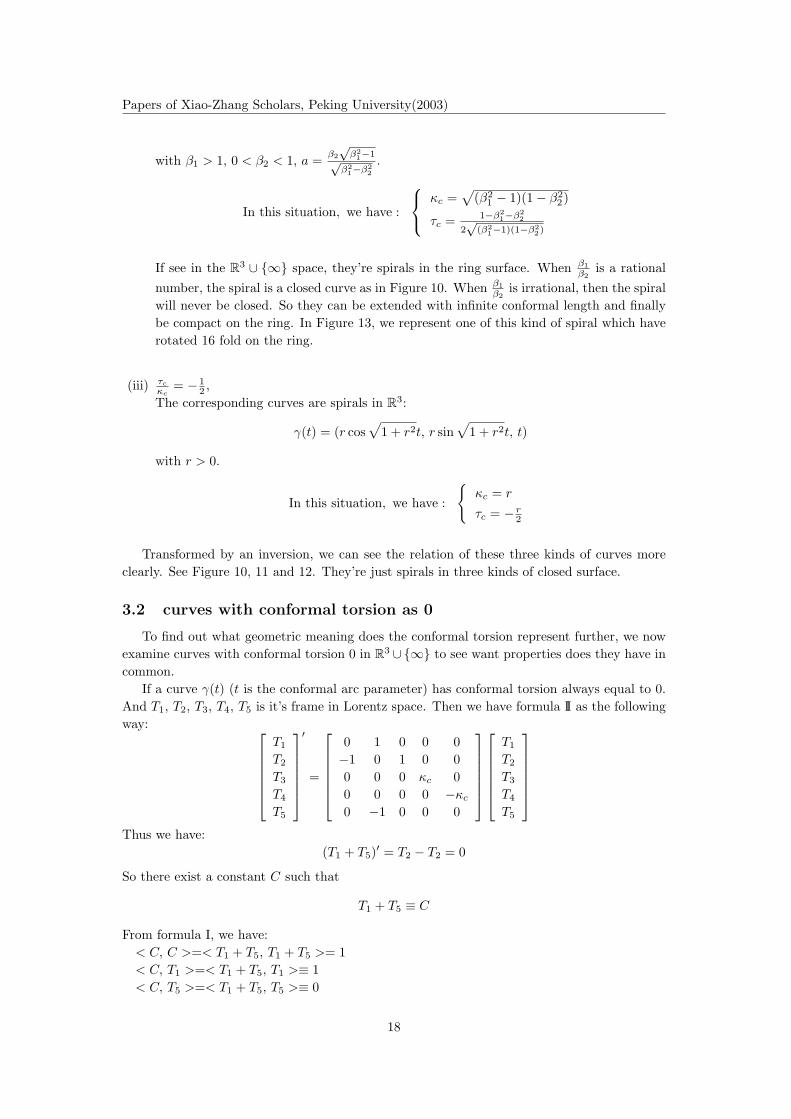
2 .The corresponding curves are spirals on the cone of R3 as in Figure 9:

γ(t) = eαt(a cos βt, a sinβt,√

1− a2)

with α > 0, β > 1, a = αβ

√β2−1α2+1 .

In this situation, we have :

κc =√

(β2 − 1)(α2 + 1)

τc = α2−β2+1

2√

(β2−1)(α2+1)

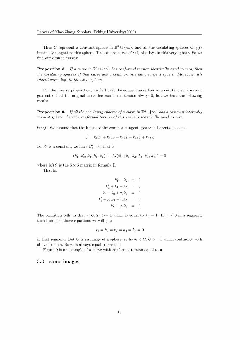
(ii) τc

κc< − 1

2 ,The corresponding curves are spirals in C× C as in Figure 9:

γ(t) = (aeiβ1t,√

1− a2eiβ2t)

17


with β1 > 1, 0 < β2 < 1, a = β2

√β21−1√

β21−β2

2

.


κc =√

(β21 − 1)(1− β2

2)

τc = 1−β21−β2

2

2√

(β21−1)(1−β2

2)

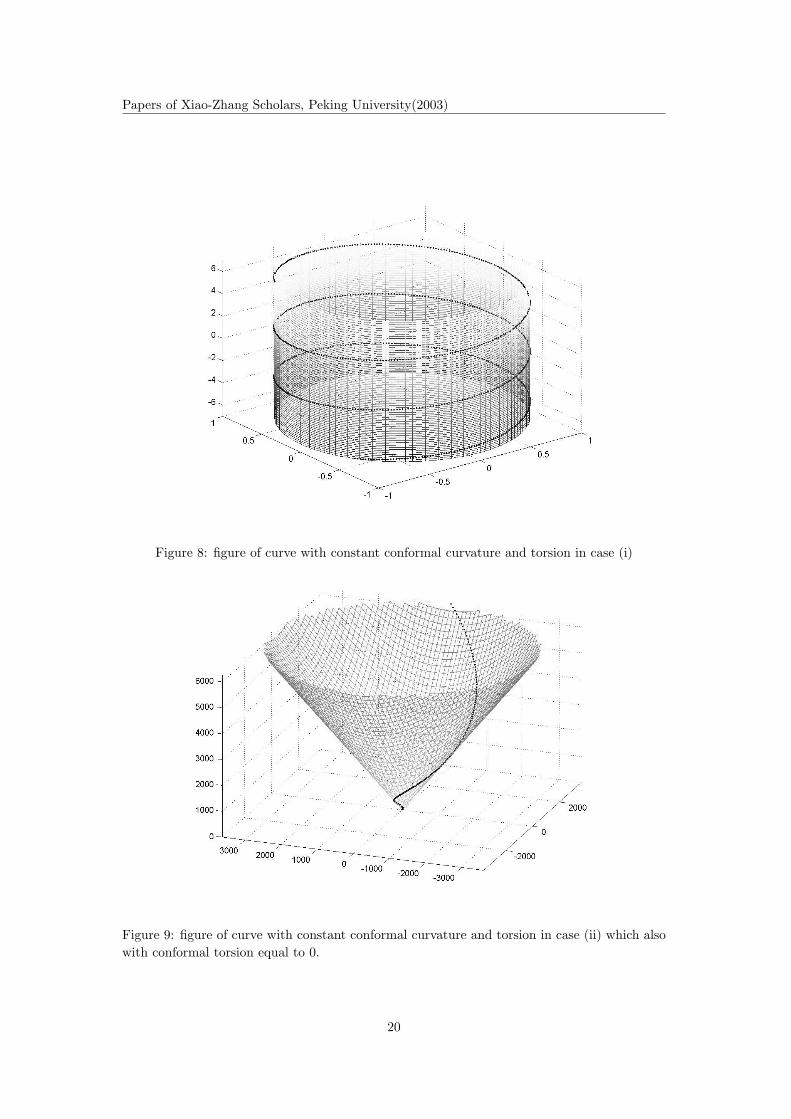
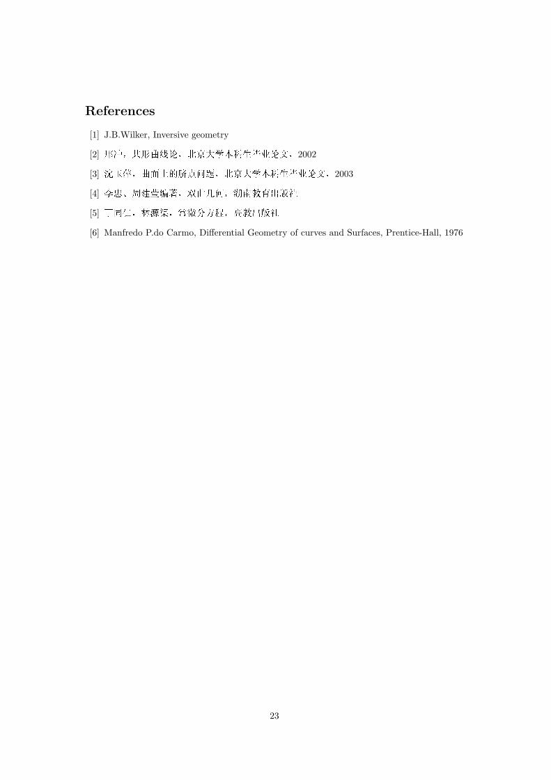
If see in the R3 ∪ {∞} space, they’re spirals in the ring surface. When β1β2

is a rationalnumber, the spiral is a closed curve as in Figure 10. When β1

β2is irrational, then the spiral

will never be closed. So they can be extended with infinite conformal length and finallybe compact on the ring. In Figure 13, we represent one of this kind of spiral which haverotated 16 fold on the ring.

(iii) τc

κc= − 1

2 ,The corresponding curves are spirals in R3:

γ(t) = (r cos√

1 + r2t, r sin√

1 + r2t, t)

with r > 0.


{κc = r

τc = − r2

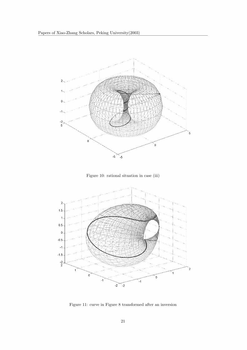
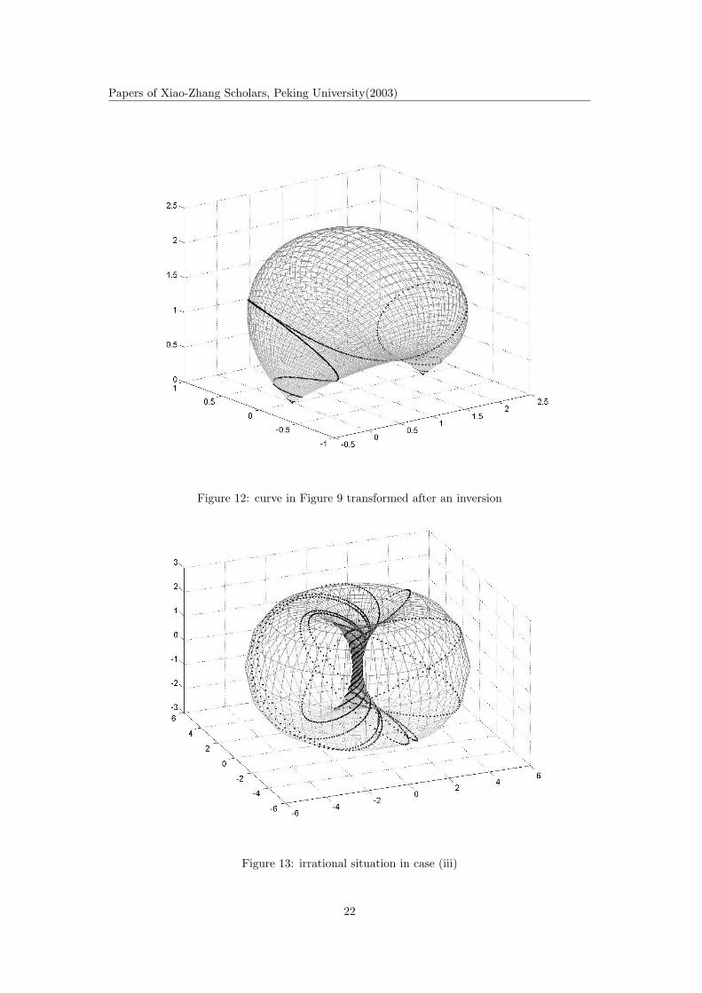
Transformed by an inversion, we can see the relation of these three kinds of curves moreclearly. See Figure 10, 11 and 12. They’re just spirals in three kinds of closed surface.

3.2 curves with conformal torsion as 0

To find out what geometric meaning does the conformal torsion represent further, we nowexamine curves with conformal torsion 0 in R3 ∪{∞} to see want properties does they have incommon.

If a curve γ(t) (t is the conformal arc parameter) has conformal torsion always equal to 0.And T1, T2, T3, T4, T5 is it’s frame in Lorentz space. Then we have formula II as the followingway:

T1

T2

T3

T4

T5

′

=

0 1 0 0 0−1 0 1 0 00 0 0 κc 00 0 0 0 −κc

0 −1 0 0 0

T1

T2

T3

T4

T5

Thus we have:

(T1 + T5)′ = T2 − T2 = 0

So there exist a constant C such that

T1 + T5 ≡ C

From formula I, we have:< C, C >=< T1 + T5, T1 + T5 >= 1< C, T1 >=< T1 + T5, T1 >≡ 1< C, T5 >=< T1 + T5, T5 >≡ 0

18


Thus C represent a constant sphere in R3 ∪ {∞}, and all the osculating spheres of γ(t)internally tangent to this sphere. The educed curve of γ(t) also lays in this very sphere. So wefind our desired curves:

Proposition 8. If a curve in R3 ∪ {∞} has conformal torsion identically equal to zero, thenthe osculating spheres of that curve has a common internally tangent sphere. Moreover, it’seduced curve lays in the same sphere.

For the inverse proposition, we find that the educed curve lays in a constant sphere can’tguarantee that the original curve has conformal torsion always 0, but we have the followingresult:

Proposition 9. If all the osculating spheres of a curve in R3∪{∞} has a common internallytangent sphere, then the conformal torsion of this curve is identically equal to zero.

Proof. We assume that the image of the common tangent sphere in Lorentz space is

C = k1T1 + k2T2 + k3T3 + k4T4 + k5T5

For C is a constant, we have C ′t = 0, that is

(k′1, k′2, k′3, k′4, k′5)τ + M(t) · (k1, k2, k3, k4, k5)τ = 0

where M(t) is the 5× 5 matrix in formula II.That is:

k′1 − k2 = 0

k′2 + k1 − k5 = 0

k′3 + k2 + τck4 = 0

k′4 + κck3 − τck5 = 0

k′5 − κck4 = 0

The condition tells us that < C, T1 >≡ 1 which is equal to k1 ≡ 1. If τc 6= 0 in a segment,then from the above equations we will get:

k1 = k2 = k3 = k4 = k5 = 0

in that segment. But C is an image of a sphere, so have < C, C >= 1 which contradict withabove formula. So τc is always equal to zero. �

Figure 9 is an example of a curve with conformal torsion equal to 0.

3.3 some images

19


Figure 8: figure of curve with constant conformal curvature and torsion in case (i)

Figure 9: figure of curve with constant conformal curvature and torsion in case (ii) which alsowith conformal torsion equal to 0.

20


Figure 10: rational situation in case (iii)

Figure 11: curve in Figure 8 transformed after an inversion

21


Figure 12: curve in Figure 9 transformed after an inversion

Figure 13: irrational situation in case (iii)

22

References

[1] J.B.Wilker, Inversive geometry

[2] 0À§�/�Ø§�®�Æ��).�Ø©§2002

[3] !�±§¡þ�ß:¯K§�®�Æ��).�Ø©§2003

[4] o§!±ïC?Í§VAÛ§�H��Ñ��

[5] ¶Ó;§� ±§~�©�§§p�Ñ��

[6] Manfredo P.do Carmo, Differential Geometry of curves and Surfaces, Prentice-Hall, 1976

23

Documents

Invariant of curves under Möbius group in 3-dimensional …dean.pku.edu.cn/bksky/2000xzjjlwjlk/5.pdf · group in 3-dimensional space ... We define a complete Möbius invariant