Embed Size (px)
Citation preview
University of Applied Sciences Bremerhaven
Simulation and Process Control[ PDV / PEET9 ]
Revision: V1.1
E---Mail: [email protected]
Date: September 2003
S Part 1: Process Modeling
D---27568 Bremerhaven
Tel: +49 471 48 23 --- 415FAX: +49 471 48 23 --- 418
Prof. Dr.-Ing. Kai MüllerUniv. of Appl. Sciences BremerhavenInstitute for Electrical Engineering and ControlAn der Karlstadt 8
S Part 3: Process Control
S Part 4: Advanced Controller Design (IMC, optional MPC)
S Part 2: Simulation
Course Material
PDV / PEET9 Univ. of Appl. Sciences BremerhavenI
I Introductory Notes
Process Control has a great impact on quality and safety in industrial production. It istherefore important for a process engineer to have a sound knowledge of control principles.
Closely related to control is the modeling of processes. Many modern controllers aremodel-based. The processmodel can be also be used to simulate the process and the closedloopwithout risking harmful experiments with real systems. Amodel is also a very valuabletool to improve the “controllability” (the best dynamic performance of a system underclosed loop control) of a process.
In this course we will cover the following topics (theoretically and in the lab):
S Modelling of essential process elements
S Process Simulation using MATLAB/Simulink (optional HYSYS)
S Simplifying models for control purposes
S Standard industrial controllers
S SISO closed loops and stability
S Internal model control (IMC)
S Simulation of closed loops
S Option: Model predictive control (MPC)
I.I Course Material
The most recent course material is available on the web site:
http://www1.hs---bremerhaven.de/kmueller/
I hope that everybody in my class enjoys the introduction in this fascinating subject.
Bremerhaven, September 2003 Kai Müller<[email protected]>
Tel: (0471) 4823 --- 415
PDV / PEET9 Univ. of Appl. Sciences Bremerhaven --- IAEII
II Table of Contents
1 Process Modeling 1. . . . . . . . . . . . . . . . . . . . . . . . . . . . . . . . . . . . . . . . . . . . . . . . . .
1.1 First Model: Gravity flow tank 1. . . . . . . . . . . . . . . . . . . . . . . . . . . . . . . . . .
1.2 Control of the flow tank 5. . . . . . . . . . . . . . . . . . . . . . . . . . . . . . . . . . . . . . .
2 Modeling --- Systematic Approach 6. . . . . . . . . . . . . . . . . . . . . . . . . . . . . . . . . . . .
2.1 Model of a physical situation 6. . . . . . . . . . . . . . . . . . . . . . . . . . . . . . . . . . .
3 Analytical solutions of differential equations 7. . . . . . . . . . . . . . . . . . . . . . . . . . .
4 Simulator (numerical simulation) 8. . . . . . . . . . . . . . . . . . . . . . . . . . . . . . . . . . . . .
4.1 Principle of operation 8. . . . . . . . . . . . . . . . . . . . . . . . . . . . . . . . . . . . . . . . .
4.2 Example: numerical integration of the gravity flow tank model(Euler formula) 9. . . . . . . . . . . . . . . . . . . . . . . . . . . . . . . . . . . . . . . . . . . . . .
5 Modeling of a Continuous Stirred Tank Reactor (CSTR) 10. . . . . . . . . . . . . . . . .
5.1 Example: Modeling a simple CSTR 12. . . . . . . . . . . . . . . . . . . . . . . . . . . . .
6 Endothermal and Exothermal Chemical Reactions 14. . . . . . . . . . . . . . . . . . . . . .
7 Modeling a Nonisothermal CSTR 17. . . . . . . . . . . . . . . . . . . . . . . . . . . . . . . . . . . .
8 Linearization 20. . . . . . . . . . . . . . . . . . . . . . . . . . . . . . . . . . . . . . . . . . . . . . . . . . . . . .
8.1 Linearization of the gravity flow tank 21. . . . . . . . . . . . . . . . . . . . . . . . . . . .
8.2 Modern Control Approach (Feedback Linearization)(this is the symbol for extremely hard stuff) 22. . . . . . . . . . . . . . . . . . . . . .
9 Perturbation Variables (nothing really new) 23. . . . . . . . . . . . . . . . . . . . . . . . . . . .
9.1 Exercise: Linearization of the Arrhenius Nonlinearity 24. . . . . . . . . . . . . .
10 Transfer Function 26. . . . . . . . . . . . . . . . . . . . . . . . . . . . . . . . . . . . . . . . . . . . . . . . . .
10.1 Signal Representation in Frequency Domain (Laplace-Transform) 26. . .
10.2 Exercises 28. . . . . . . . . . . . . . . . . . . . . . . . . . . . . . . . . . . . . . . . . . . . . . . . . . . .
10.3 Important Laplace Function Computation Rules 29. . . . . . . . . . . . . . . . . .
10.4 Deriving the Transfer Function from Differential Equations 29. . . . . . . . .
10.4.1 Frequency Domain Model of the Gravity Flow Tank 30. . . . . . . . .
10.4.2 EXERCISE: Comparison of the Nonlinear and the Linearized Model31
PDV / PEET9 Univ. of Appl. Sciences Bremerhaven --- IAEIII
11 Level Control for the Gravity Flow Tank 32. . . . . . . . . . . . . . . . . . . . . . . . . . . . . . .
12 Calculation with Transfer Functions and Signals 33. . . . . . . . . . . . . . . . . . . . . . . . .
12.1 Serial Connection (Multiplication) 34. . . . . . . . . . . . . . . . . . . . . . . . . . . . . .
12.2 Parallel Connection (Addition) 35. . . . . . . . . . . . . . . . . . . . . . . . . . . . . . . . .
12.3 Closed Loops 35. . . . . . . . . . . . . . . . . . . . . . . . . . . . . . . . . . . . . . . . . . . . . . . .
13 Elementary Transfer Functions 38. . . . . . . . . . . . . . . . . . . . . . . . . . . . . . . . . . . . . . .
13.1 Proportional gain 38. . . . . . . . . . . . . . . . . . . . . . . . . . . . . . . . . . . . . . . . . . . . .
13.2 Integrator 39. . . . . . . . . . . . . . . . . . . . . . . . . . . . . . . . . . . . . . . . . . . . . . . . . . .
13.3 Differentiation 40. . . . . . . . . . . . . . . . . . . . . . . . . . . . . . . . . . . . . . . . . . . . . . .
13.4 First Order Lag 41. . . . . . . . . . . . . . . . . . . . . . . . . . . . . . . . . . . . . . . . . . . . . .
13.5 Lead-Lag Element 42. . . . . . . . . . . . . . . . . . . . . . . . . . . . . . . . . . . . . . . . . . .
14 Frequency Analysis of Transfer Functions 44. . . . . . . . . . . . . . . . . . . . . . . . . . . . . .
14.1 General Form of a Real Rational Transfer Function 44. . . . . . . . . . . . . . .
14.2 Frequency Response 45. . . . . . . . . . . . . . . . . . . . . . . . . . . . . . . . . . . . . . . . . .
14.2.1 Frequency Response example 47. . . . . . . . . . . . . . . . . . . . . . . . . . . .
14.3 Bode Diagram 48. . . . . . . . . . . . . . . . . . . . . . . . . . . . . . . . . . . . . . . . . . . . . . .
14.4 Nyquist Diagram 49. . . . . . . . . . . . . . . . . . . . . . . . . . . . . . . . . . . . . . . . . . . . .
15 Poles and Zeros 50. . . . . . . . . . . . . . . . . . . . . . . . . . . . . . . . . . . . . . . . . . . . . . . . . . .
15.1 Example: Transformation into Pole-Zero Form 51. . . . . . . . . . . . . . . . . . .
15.2 Frequency Response of the Pole-Zero Form 51. . . . . . . . . . . . . . . . . . . . . .
15.3 Dependency of the Magnitude of the Bode Diagram on theZeros and Poles 54. . . . . . . . . . . . . . . . . . . . . . . . . . . . . . . . . . . . . . . . . . . . . .
15.3.1 All-pass Transfer Function 55. . . . . . . . . . . . . . . . . . . . . . . . . . . . . .
16 Non Real Rational Transfer Functions 56. . . . . . . . . . . . . . . . . . . . . . . . . . . . . . . . .
17 Stability 58. . . . . . . . . . . . . . . . . . . . . . . . . . . . . . . . . . . . . . . . . . . . . . . . . . . . . . . . . .
18 Closed Loop Stability 60. . . . . . . . . . . . . . . . . . . . . . . . . . . . . . . . . . . . . . . . . . . . . . .
18.1 Example: Stability of a Closed Loop system 61. . . . . . . . . . . . . . . . . . . . . .
18.2 Closed Loop Stability and the Nyquist Diagram 63. . . . . . . . . . . . . . . . . . .
18.3 Phase and Gain Distance 65. . . . . . . . . . . . . . . . . . . . . . . . . . . . . . . . . . . . . .
19 Controller Design by Specification of Gain and Phase Distances 67. . . . . . . . . . .
19.1 Example: Controlling a 3. Order Lag with a Proportional Controller 68. .
PDV / PEET9 Univ. of Appl. Sciences Bremerhaven --- IAEIV
19.1.1 Design K for Gain Distance rd = 0.8 68. . . . . . . . . . . . . . . . . . . .
19.1.2 Design K for Phase Distance Ψd = π/3 70. . . . . . . . . . . . . . . . . .
20 Controller Design 72. . . . . . . . . . . . . . . . . . . . . . . . . . . . . . . . . . . . . . . . . . . . . . . . . .
20.1 Controller Types 72. . . . . . . . . . . . . . . . . . . . . . . . . . . . . . . . . . . . . . .
20.2 Selecting the Suitable Controller 74. . . . . . . . . . . . . . . . . . . . . . . . . . . . . . . .
20.3 Standard Configurations 75. . . . . . . . . . . . . . . . . . . . . . . . . . . . . . . . . . . . . . .
20.3.1 First Order System 75. . . . . . . . . . . . . . . . . . . . . . . . . . . . . . . . . . . . .
20.3.2 Integrator Process 76. . . . . . . . . . . . . . . . . . . . . . . . . . . . . . . . . . . . .
20.3.3 Second Order System 77. . . . . . . . . . . . . . . . . . . . . . . . . . . . . . . . . .
20.3.4 Other Systems 79. . . . . . . . . . . . . . . . . . . . . . . . . . . . . . . . . . . . . . . . .
21 Heuristic Methods 79. . . . . . . . . . . . . . . . . . . . . . . . . . . . . . . . . . . . . . . . . . . . . . . . .
21.1 Tu-Tg-Methods (Tu-T0-Methods) 80. . . . . . . . . . . . . . . . . . . . . . . . . . . . . . .
21.2 Ziegler-Nichols-Type Methods 81. . . . . . . . . . . . . . . . . . . . . . . . . . . . . . . . . .
22 Level Control of an Uncoupled Three-Tank System 83. . . . . . . . . . . . . . . . . . . . . .
22.1 Mechanical Control of the Simplified System 83. . . . . . . . . . . . . . . . . . . . .
22.2 P and I Control of the Complete Nonlinear System 84. . . . . . . . . . . . . . . .
23 Frequency and Time domain and Analysis of LTI (Linear Time Invariant)Systems 85. . . . . . . . . . . . . . . . . . . . . . . . . . . . . . . . . . . . . . . . . . . . . . . . . . . . . . . . . .
24 Impact of Zeros and Poles on Process Properties 86. . . . . . . . . . . . . . . . . . . . . . . .
25 References 87. . . . . . . . . . . . . . . . . . . . . . . . . . . . . . . . . . . . . . . . . . . . . . . . . . . . . . . .
PDV / PEET9 Univ. of Appl. Sciences Bremerhaven1
1 Process Modeling
Modeling requires understanding of operation, objectives, constraints and uncertainties ofthe process.
A model for control purposes must describe the dynamic behavior (not only thesteady-state). It should be as simple as possible in order to keep the number of parameterssmall.
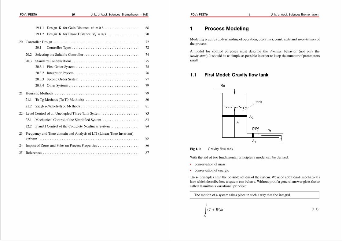
1.1 First Model: Gravity flow tank
q0
h
q1
A1
A0
tank
pipe
Fig 1.1: Gravity flow tank
With the aid of two fundamental principles a model can be derived:
S conservation of mass
S conservation of energy.
These principles limit the possible actions of the system. We need additional (mechanical)laws which describe how a system can behave. Without proof a general answer gives the socalled Hamilton’s variational principle:
The motion of a system takes place in such a way that the integral
t2
t1
(T+W)dt (1.1)
PDV / PEET9 Univ. of Appl. Sciences Bremerhaven2
is an extremum (Hamilton’s variational principle).
T denotes the total kinetic energy and W denotes the work of the external forces. Don’tget headaches with equation (1.1) --- we will not use it here. I introduce this remarkablygeneral formula just to present a complete set of formulas to describe system in fig. 1.1.
We know from elementary mechanics that the fluid from the tank flows out of the pipe dueto gravitational force.We assume an incompressible fluidwith densityρ. TheVolume in thetank is given by
V0= A0h (1.2)
and the total mass in the tank is therefore
m= ÃA0h . (1.3)
If the level of the tank changes by a small amount ∆h the potential energy change is
∆L= mg∆h= ÃA0hg ∆h . (1.4)
If the area A0 is very large compared to A1 then the change of h is very small comparedto the speed of the fluid in the pipe. This means we have a kinetic energy only on the pipe
∆T= 12∆m v2 , (1.5)
where
∆m=− ÃA0 ∆h . (1.6)
(∆h is negative). With (1.6) equation (1.5) can be written as
∆T=− 12ÃA0 ∆h v2 . (1.7)
The sum of both energies must be zero
∆L+ ∆T= ÃA0hg ∆h−12ÃA0 ∆h v
2= 0 . (1.8)
Solving (1.8) for the speed leads to
v= 2gh . (1.9)
This result is a special form of the “Bernoulli” equation. The velocity of the fluid in the pipedepends not on the density ρ or the area A0. Now we can derive the output flow
q1= A1v= A1 2gh . (1.10)
The input flow q0 is assumed to be an input value. Our System has thus the followingstructure.
PDV / PEET9 Univ. of Appl. Sciences Bremerhaven3
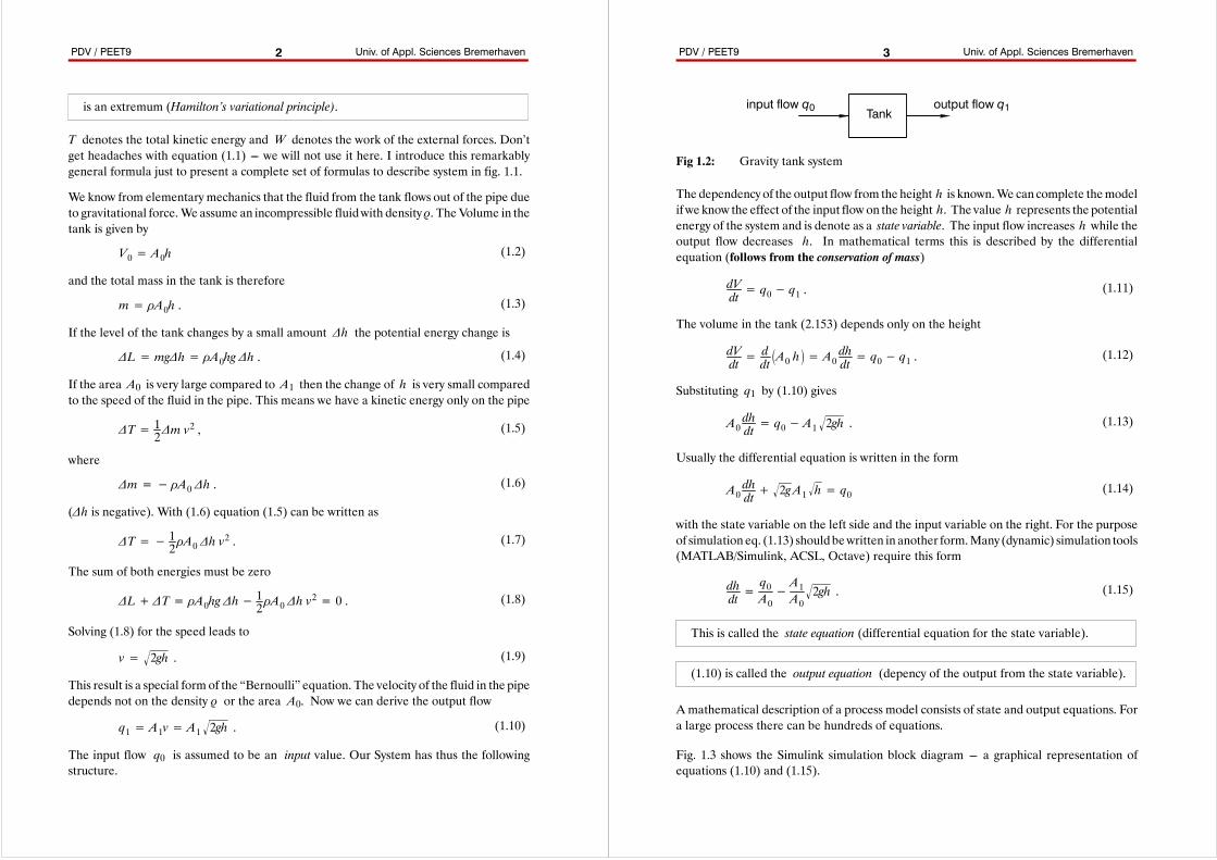
Tankinput flow q0 output flow q1
Fig 1.2: Gravity tank system
The dependency of the output flow from the height h is known.We can complete themodelif we know the effect of the input flow on the height h. The value h represents the potentialenergy of the system and is denote as a state variable. The input flow increases h while theoutput flow decreases h. In mathematical terms this is described by the differentialequation (follows from the conservation of mass)
dVdt= q0− q1 . (1.11)
The volume in the tank (2.153) depends only on the height
dVdt= ddtA0 h = A0 dhdt = q0− q1 .
(1.12)
Substituting q1 by (1.10) gives
A0dhdt= q0− A1 2gh . (1.13)
Usually the differential equation is written in the form
A0dhdt+ 2g A1 h
= q0 (1.14)
with the state variable on the left side and the input variable on the right. For the purposeof simulation eq. (1.13) should bewritten in another form.Many (dynamic) simulation tools(MATLAB/Simulink, ACSL, Octave) require this form
dhdt=q0A0−A1A02gh . (1.15)
This is called the state equation (differential equation for the state variable).
(1.10) is called the output equation (depency of the output from the state variable).
A mathematical description of a process model consists of state and output equations. Fora large process there can be hundreds of equations.
Fig. 1.3 shows the Simulink simulation block diagram --- a graphical representation ofequations (1.10) and (1.15).

PDV / PEET9 Univ. of Appl. Sciences Bremerhaven4
Fig 1.3: Simulink block diagram of the gravity flow tank
Fig 1.4: Simulation result for a pulse-type input flow rate q0
PDV / PEET9 Univ. of Appl. Sciences Bremerhaven5
It can be seen that there is a close relation between the input and output flow rate. But theform of the curves differ very much. This is typical for a dynamic system.
Often the steady-state (as time goes towards infinity) is important for operation of theprocess. This follows easily from the differential equations. A steady-state arrives when allsignals (especially the state variables) remain constant. We just have to solve the stateequations for the case that all derivatives are zero.
In our example we arrive from (1.13) to
0= q0− A1 2gh . (1.16)
If the input flow rate q0 is constant, than as time goes towards infinity the constant heightbecomes
hss=q202gA21
(1.17)
For this height the input and output flow rates are identical. Of course, the process designengineer must ensure that this steady-state tank level is less than the tank height!
1.2 Control of the flow tank
If the behavior of the flow tank is not suitable for a specific process the flow tank propertiescan be changed to meet the demands. A typical example is the control of the tank level h.
q0
h
q1
A1
A0
control valvepump
level sensor
valve
controllerhref
h
---
Fig 1.5: Level control of the gravity flow tank
PDV / PEET9 Univ. of Appl. Sciences Bremerhaven6
The tank level is measured by a sensor. The measurement is compared to a referencevalue href . The difference (control error) is feed to the controller which generates the theinput signal for a control valve to change the input flow rate q0. If the controller is properlydesigned the tank level remains nearly constant regardless of the output flow rate q1. Thesignal q1 can be regarded as a disturbance value for the tank level h.
As we can see, a controller can change the original system’s behavior so that it becomesmuchmore suitable for technical applications. A poorly designed controlled system can beworse than an uncontrolled system. In our case a bad controller may cause heavyoscillations in the tank level.
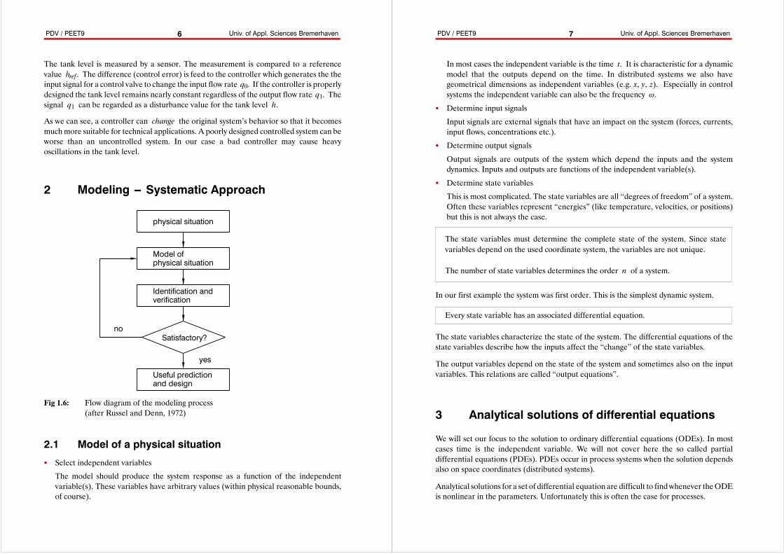
2 Modeling -- Systematic Approach
physical situation
Model ofphysical situation
Identification andverification
Satisfactory?no
yes
Useful predictionand design
Fig 1.6: Flow diagram of the modeling process(after Russel and Denn, 1972)
2.1 Model of a physical situation
S Select independent variables
The model should produce the system response as a function of the independentvariable(s). These variables have arbitrary values (within physical reasonable bounds,of course).
PDV / PEET9 Univ. of Appl. Sciences Bremerhaven7
In most cases the independent variable is the time t. It is characteristic for a dynamicmodel that the outputs depend on the time. In distributed systems we also havegeometrical dimensions as independent variables (e.g. x, y, z). Especially in controlsystems the independent variable can also be the frequency ω.
S Determine input signals
Input signals are external signals that have an impact on the system (forces, currents,input flows, concentrations etc.).
S Determine output signals
Output signals are outputs of the system which depend the inputs and the systemdynamics. Inputs and outputs are functions of the independent variable(s).
S Determine state variables
This is most complicated. The state variables are all “degrees of freedom” of a system.Often these variables represent “energies” (like temperature, velocities, or positions)but this is not always the case.
The state variables must determine the complete state of the system. Since statevariables depend on the used coordinate system, the variables are not unique.
The number of state variables determines the order n of a system.
In our first example the system was first order. This is the simplest dynamic system.
Every state variable has an associated differential equation.
The state variables characterize the state of the system. The differential equations of thestate variables describe how the inputs affect the “change” of the state variables.
The output variables depend on the state of the system and sometimes also on the inputvariables. This relations are called “output equations”.
3 Analytical solutions of differential equations
We will set our focus to the solution to ordinary differential equations (ODEs). In mostcases time is the independent variable. We will not cover here the so called partialdifferential equations (PDEs). PDEs occur in process systems when the solution dependsalso on space coordinates (distributed systems).
Analytical solutions for a set of differential equation are difficult to findwhenever theODEis nonlinear in the parameters. Unfortunately this is often the case for processes.
PDV / PEET9 Univ. of Appl. Sciences Bremerhaven8
If the input functions are not mathematical functions (like step, sine etc.) an analyticalsolution is not possible. It is therefore common practice to perform a numerical integrationof ODEs and PDEs, respectively.
4 Simulator (numerical simulation)
A numerical simulation can easily solve any number of (nonlinear) ODEs with arbitraryinput signal waveforms. However, numerical simulations do not provide exact solutions.Instead they approximate the exact solution by an finite number of discrete simulationsteps. As a rule of thumb one may say that the smaller the step size the more precise is thenumerical integration. On the other hand a small step size results in a high computationtime.
4.1 Principle of operation
Adigital simulator discretizes the time axis (or whatever the independent variable is). Thestep size is denoted as h. From the ODE the derivative is known. From the current valueof the state variable the simulation performs a single step. After one step the time t0 isadvanced to t0 + stepsize.
t0 := t0+ h . (1.18)
t
x
t0 t0+h
xk+1
xk
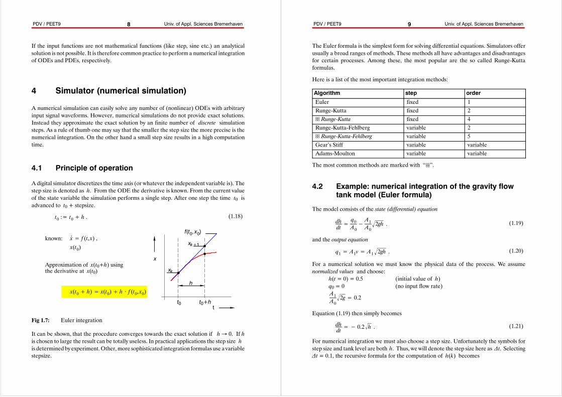
known: x. = f (t, x) ,x(t0)
Approximation of x(t0+h) usingthe derivative at x(t0)
x(t0+ h)= x(t0)+ h ⋅ f (t0, x0)
f(t0, x0)
h
Fig 1.7: Euler integration
It can be shown, that the procedure converges towards the exact solution if h→ 0. If his chosen to large the result can be totally useless. In practical applications the step size his determinedby experiment.Other,more sophisticated integration formulas use a variablestepsize.
PDV / PEET9 Univ. of Appl. Sciences Bremerhaven9
The Euler formula is the simplest form for solving differential equations. Simulators offerusually a broad ranges of methods. These methods all have advantages and disadvantagesfor certain processes. Among these, the most popular are the so called Runge-Kuttaformulas.
Here is a list of the most important integration methods:
Algorithm step orderEuler fixed 1Runge-Kutta fixed 2U Runge-Kutta fixed 4Runge-Kutta-Fehlberg variable 2U Runge-Kutta-Fehlberg variable 5Gear’s Stiff variable variableAdams-Moulton variable variable
The most common methods are marked with “U”.
4.2 Example: numerical integration of the gravity flowtank model (Euler formula)
The model consists of the state (differential) equation
dhdt=q0A0−A1A02gh . (1.19)
and the output equation
q1= A1v= A1 2gh . (1.20)
For a numerical solution we must know the physical data of the process. We assumenormalized values and choose:
h(t = 0) = 0.5 (initial value of h)q0 = 0 (no input flow rate)A1A02g = 0.2
Equation (1.19) then simply becomes
dhdt=− 0.2 h . (1.21)
For numerical integration we must also choose a step size. Unfortunately the symbols forstep size and tank level are both h. Thus, we will denote the step size here as ∆t. Selecting∆t = 0.1, the recursive formula for the computation of h(k) becomes
PDV / PEET9 Univ. of Appl. Sciences Bremerhaven10
h(t0+ ∆t)= h(t0)+dhdth(t0)
∆t= h(t0)− 0.02 h(t0 ) . (1.22)
As you can see, you only need the (known) information on h(t0) to calculate h(t0+∆t).These kind of integrationmethods are called explicit formulas. The next step is the advancein time
t0 := t0+ ∆t . (1.23)
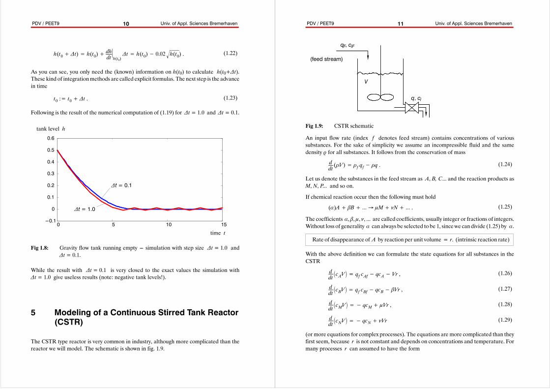
Following is the result of the numerical computation of (1.19) for ∆t = 1.0 and ∆t = 0.1.
0 5 10 15---0.1
0
0.1
0.2
0.3
0.4
0.5
0.6
time t
tank level h
∆t = 1.0
∆t = 0.1
Fig 1.8: Gravity flow tank running empty --- simulation with step size ∆t = 1.0 and∆t = 0.1.
While the result with ∆t = 0.1 is very closed to the exact values the simulation with∆t = 1.0 give useless results (note: negative tank levels!).
5 Modeling of a Continuous Stirred Tank Reactor(CSTR)
The CSTR type reactor is very common in industry, although more complicated than thereactor we will model. The schematic is shown in fig. 1.9.
PDV / PEET9 Univ. of Appl. Sciences Bremerhaven11
q, ci
qF, ciF
V
(feed stream)
Fig 1.9: CSTR schematic
An input flow rate (index f denotes feed stream) contains concentrations of varioussubstances. For the sake of simplicity we assume an incompressible fluid and the samedensity ρ for all substances. It follows from the conservation of mass
ddt(ÃV)= Ãf qf− Ãq . (1.24)
Let us denote the substances in the feed stream as A, B, C... and the reaction products asM, N, P... and so on.
If chemical reaction occur then the following must hold
(α)A+ βB+ → μM+ νN+ . (1.25)
The coefficients α, β, μ, ν, ... are called coefficients, usually integer or fractions of integers.Without loss of generality α can always be selected to be 1, sincewe candivide (1.25) by α.
Rate of disappearance of A by reaction per unit volume = r. (intrinsic reaction rate)
With the above definition we can formulate the state equations for all substances in theCSTR
ddtcAV = qf cAf− qcA− Vr , (1.26)
ddtcBV = qf cBf− qcB− βVr , (1.27)
ddtcMV = − qcM+ μVr , (1.28)
ddtcNV = − qcN+ νVr (1.29)
(or more equations for complex processes). The equations are more complicated than theyfirst seem, because r is not constant and depends on concentrations and temperature. Formany processes r can assumed to have the form
PDV / PEET9 Univ. of Appl. Sciences Bremerhaven12
r= k caA cbB , (1.30)
where k depends on temperature and the exponents are strongly related to α and β.(sometimes they are identical a = α, b = β).
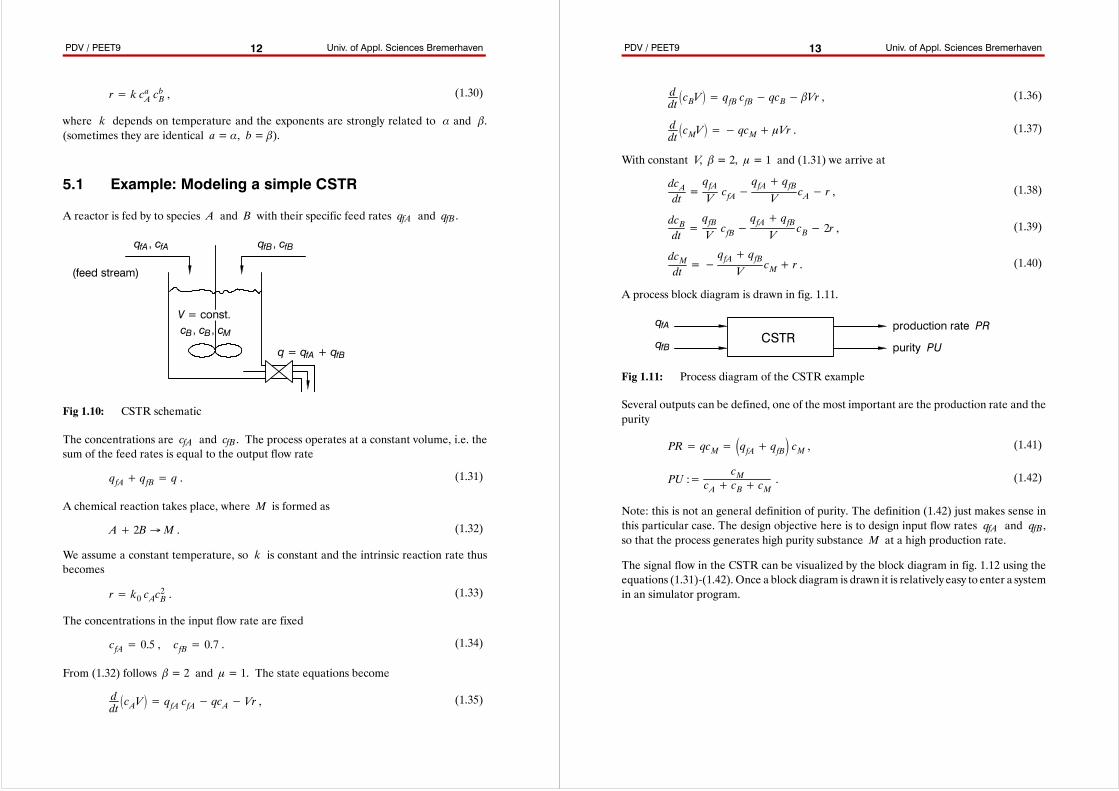
5.1 Example: Modeling a simple CSTR
A reactor is fed by to species A and B with their specific feed rates qfA and qfB .
q = qfA + qfB
qfA , cfA
V = const.
(feed stream)
qfB , cfB
cB , cB , cM
Fig 1.10: CSTR schematic
The concentrations are cfA and cfB . The process operates at a constant volume, i.e. thesum of the feed rates is equal to the output flow rate
qfA+ qfB= q . (1.31)
A chemical reaction takes place, where M is formed as
A+ 2B→ M . (1.32)
We assume a constant temperature, so k is constant and the intrinsic reaction rate thusbecomes
r= k0 cAc2B . (1.33)
The concentrations in the input flow rate are fixed
cfA= 0.5 , cfB= 0.7 . (1.34)
From (1.32) follows β = 2 and μ = 1. The state equations become
ddtcAV = qfA cfA− qcA− Vr , (1.35)
PDV / PEET9 Univ. of Appl. Sciences Bremerhaven13
ddtcBV = qfB cfB− qcB− βVr , (1.36)
ddtcMV = − qcM+ μVr . (1.37)
With constant V, β = 2, μ = 1 and (1.31) we arrive at
dcAdt=qfAVcfA−
qfA+ qfBV
cA− r , (1.38)
dcBdt=qfBVcfB−
qfA+ qfBV
cB− 2r , (1.39)
dcMdt=−
qfA+ qfBV
cM+ r . (1.40)
A process block diagram is drawn in fig. 1.11.
CSTRqfA
qfB
production rate PR
purity PU
Fig 1.11: Process diagram of the CSTR example
Several outputs can be defined, one of the most important are the production rate and thepurity
PR= qcM= qfA+ qfB cM , (1.41)
PU :=cM
cA+ cB+ cM. (1.42)
Note: this is not an general definition of purity. The definition (1.42) just makes sense inthis particular case. The design objective here is to design input flow rates qfA and qfB ,so that the process generates high purity substance M at a high production rate.
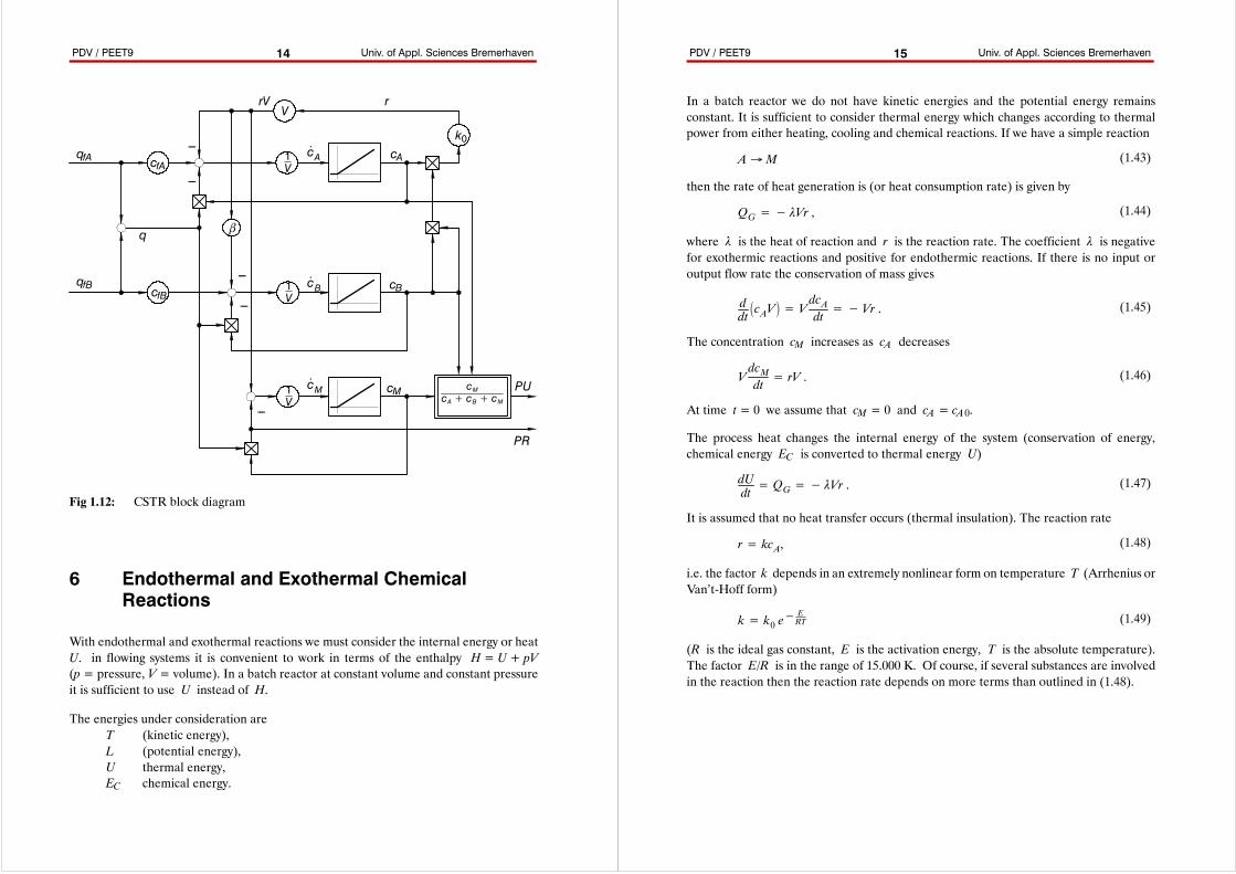
The signal flow in the CSTR can be visualized by the block diagram in fig. 1.12 using theequations (1.31)-(1.42). Once a block diagram is drawn it is relatively easy to enter a systemin an simulator program.
PDV / PEET9 Univ. of Appl. Sciences Bremerhaven14
1V
1V
1V
cfA
cfB
qfA
qfB
q
cAc.A
---
cBc.B
β
---
---
---
cMc.M
---
rV
k0
cMcA+ cB+ cM
PU
PR
rV
Fig 1.12: CSTR block diagram
6 Endothermal and Exothermal ChemicalReactions
With endothermal and exothermal reactions we must consider the internal energy or heatU. in flowing systems it is convenient to work in terms of the enthalpy H = U + pV(p = pressure, V = volume). In a batch reactor at constant volume and constant pressureit is sufficient to use U instead of H.
The energies under consideration areT (kinetic energy),L (potential energy),U thermal energy,EC chemical energy.
PDV / PEET9 Univ. of Appl. Sciences Bremerhaven15
In a batch reactor we do not have kinetic energies and the potential energy remainsconstant. It is sufficient to consider thermal energy which changes according to thermalpower from either heating, cooling and chemical reactions. If we have a simple reaction
A→ M (1.43)
then the rate of heat generation is (or heat consumption rate) is given by
QG=− λVr , (1.44)
where λ is the heat of reaction and r is the reaction rate. The coefficient λ is negativefor exothermic reactions and positive for endothermic reactions. If there is no input oroutput flow rate the conservation of mass gives
ddtcAV = V
dcAdt=− Vr . (1.45)
The concentration cM increases as cA decreases
VdcMdt= rV . (1.46)
At time t = 0 we assume that cM = 0 and cA = cA0.
The process heat changes the internal energy of the system (conservation of energy,chemical energy EC is converted to thermal energy U)
dUdt= QG=− λVr . (1.47)
It is assumed that no heat transfer occurs (thermal insulation). The reaction rate
r= kcA, (1.48)
i.e. the factor k depends in an extremely nonlinear form on temperature T (Arrhenius orVan’t-Hoff form)
k= k0 e− ERT (1.49)
(R is the ideal gas constant, E is the activation energy, T is the absolute temperature).The factor E/R is in the range of 15.000 K. Of course, if several substances are involvedin the reaction then the reaction rate depends on more terms than outlined in (1.48).
PDV / PEET9 Univ. of Appl. Sciences Bremerhaven16
0.10.20.30.40.50.60.70.80.91
1 2 3 4 5 6 7 8 9 10
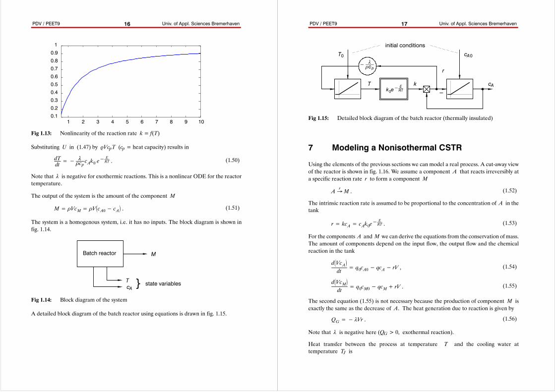
Fig 1.13: Nonlinearity of the reaction rate k = f(T)
Substituting U in (1.47) by ρVcpT (cp = heat capacity) results in
dTdt=− λ
Ãcp cAk0 e− ERT . (1.50)
Note that λ is negative for exothermic reactions. This is a nonlinear ODE for the reactortemperature.
The output of the system is the amount of the component M
M= ÃVcM= ÃVcA0− cA . (1.51)
The system is a homogenous system, i.e. it has no inputs. The block diagram is shown infig. 1.14.
Batch reactor M
TcA } state variables
Fig 1.14: Block diagram of the system
A detailed block diagram of the batch reactor using equations is drawn in fig. 1.15.
PDV / PEET9 Univ. of Appl. Sciences Bremerhaven17
− λÃcp
k0e− ERT
r
---kT cA
cA0T0
initial conditions
Fig 1.15: Detailed block diagram of the batch reactor (thermally insulated)
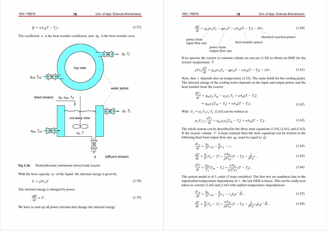
7 Modeling a Nonisothermal CSTR
Using the elements of the previous sections we can model a real process. A cut-away viewof the reactor is shown in fig. 1.16. We assume a component A that reacts irreversibly ata specific reaction rate r to form a component M
A→r M . (1.52)
The intrinsic reaction rate is assumed to be proportional to the concentration of A in thetank
r= kcA= cAk0e− ERT . (1.53)
For the components A and M we can derive the equations from the conservation ofmass.The amount of components depend on the input flow, the output flow and the chemicalreaction in the tank
dVcAdt
= q0cA0− qcA− rV , (1.54)
dVcMdt
= q0cM0− qcM+ rV . (1.55)
The second equation (1.55) is not necessary because the production of component M isexactly the same as the decrease of A. The heat generation due to reaction is given by
QG=− λVr . (1.56)
Note that λ is negative here (QG > 0, exothermal reaction).
Heat transfer between the process at temperature T and the cooling water attemperature TJ is
PDV / PEET9 Univ. of Appl. Sciences Bremerhaven18
Q= ÀAHT− TJ . (1.57)
The coefficient κ is the heat transfer coefficient, and AH is the heat transfer area.
q
q0, cA0, T0(feed stream)
water jacket
top view
qJ0, TJ0
qJ, TJ
cA , T
(effluent stream)
qJ0, TJ0
qJ, TJ
cut-away view
Fig 1.16: Nonisothermal continuous stirred tank reactor
With the heat capacity cP of the liquid the internal energy is given by
U= ÃVcPT (1.58)
The internal energy is changed by power
dWdt= P . (1.59)
We have to sum up all power streams that change the internal energy
PDV / PEET9 Univ. of Appl. Sciences Bremerhaven19
dUdt= q0 ÃcPT0− qÃcPT− ÀAH(T− TJ)− λVr . (1.60)
power frominput flow rate
power fromoutput flow rate
heat transfer power
chemical reaction power
If we operate the reactor at constant volume we can use (1.58) to obtain an ODE for thereactor temperature T
ÃVcPdTdt= q0 ÃcPT0− qÃcPT− ÀAH(T− TJ)− λVr . (1.61)
Note, that r depends also on temperature (1.53). The same holds for the cooling jacket.The internal energy of the cooling water depends on the input and output power and theheat transfer from the reactor
= qJ0 ÃJTJ0− TJ + ÀAH(T− TJ) . (1.62)
dUJdt= qJ0 ÃJ TJ0− qJ ÃJ TJ+ ÀAH(T− TJ)
With UJ= ÃJ VJ cJ TJ (1.62) can be written as
ÃJ VJ cJdTJdt= qJ0 ÃJcJTJ0− TJ + ÀAH(T− TJ) . (1.63)
The whole system can be described by the three state equations (1.54), (1.61), and (1.63).If the reactor volume V is kept constant then the state equations can be written in thefollowing final form (input flow rate q0 must be equal to q)
dcAdt=q0VcA0−
qVcA− r , (1.64)
dTdt=qVT0− T −
ÀAHÃVcP
(T− TJ)−λÃcPr , (1.65)
dTJdt=qJ0VJTJ0− TJ +
ÀAHÃJVJcJ
(T− TJ) . (1.66)
The system model is of 3. order (3 state variables). The first two are nonlinear due to theexponential temperature dependency of r, the last ODE is linear. This can be easily seenwhen we rewrite (1.64) and (1.65) with explicit temperature dependencies
dcAdt=q0VcA0−
qVcA− cAk0e
− ERT , (1.67)
dTdt=qVT0− T −
ÀAHÃVcP
(T− TJ)−λÃcPcAk0e
− ERT . (1.68)
PDV / PEET9 Univ. of Appl. Sciences Bremerhaven20
As the system becomes more complex a detailed block diagram is not very helpful tounderstand the system.
8 Linearization
Controller design is much easier when a system in linear. Unfortunately most processmodels a more or less nonlinear. A function f(x) is linear when the following holds
f (ax)= a f (x) ∀ a∈ < . (1.69)
In other words: the system behavior does not depend the amplitude of x. For instance asquare root function does not satisfy (1.69)
ax = a x ≠ a x . (1.70)
Linearization of a system is the approximation of the system at a specific point ofoperation (equilibrium point, steady-state).
Any nonlinear function
y= F(u) (1.71)
where derivatives exist at x0 can be written as a Taylor-series expansion in the form
y0+ ∆y= F(u0)+∂F∂uu0∆u+ 12!
∂2F∂u2u0∆u2+ 13!
∂3F∂u3u0∆u3 (1.72)
Since y0 = F(u0) it is obvious that
∆y= ∂F∂uu0∆u+ 12!
∂2F∂u2u0∆u2+ 13!
∂3F∂u3u0∆u3 (1.73)
If ∆u is small then ∆y can be expressed as
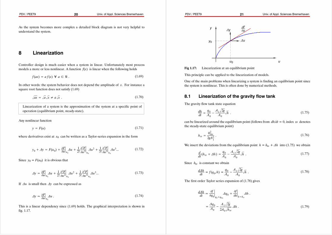
∆y≈ ∂F∂uu0∆u . (1.74)
This is a linear dependency since (1.69) holds. The graphical interpretation is shown infig. 1.17.
PDV / PEET9 Univ. of Appl. Sciences Bremerhaven21
u
y
∆u
∆y∂F∂u
u0
y0
Fig 1.17: Linearization at an equilibrium point
This principle can be applied to the linearization of models.
One of the main problems when linearizing a system is finding an equlibrium point sincethe system is nonlinear. This is often done by numerical methods.
8.1 Linearization of the gravity flow tankThe gravity flow tank state equation
dhdt=q0A0−A1 2gA0
h . (1.75)
can be linearized around the equilibrium point (follows from dh/dt = 0, index ss denotesthe steady-state equilibrium point)
hss=q20ss2gA21
. (1.76)
We insert the deviations from the equilibrium point h = hss + ∆h into (1.75) we obtain
ddt(hss+ ∆h)=
q0A0−A1 2gA0
h . (1.77)
Since hss is constant we obtain
d∆hdt= f (q0, h)=
q0A0−A1 2gA0
h . (1.78)
The first order Taylor series expansion of (1.78) gives
=∆q0A0−A1 2g
2A0 hss∆h . (1.79)
d∆hdt≈∂f∂q0q0=q0ss
∆q0+∂f∂hh=hss
∆h .
PDV / PEET9 Univ. of Appl. Sciences Bremerhaven22
The state equation is now a linear function of ∆h (and ∆q0, of course). Keep in mind thatthis is only valid if the deviation from the operating point (i.e. |∆h|) is kept relatively small.
8.2 Modern Control Approach (Feedback Linearization)
(this is the symbol for extremely hard stuff)
Feedback of signals can change a system behavior. Most processes (even complex systems)can be perfectly linearized by state variable feedback. This is called feedback linearization.The idea is quite simple: replace the nonlinear part by a new input. In the equation
dhdt=q0A0−A1 2gA0
h (1.80)
the complete right side is replaced by the new variable
v :=q0A0−A1 2gA0
h . (1.81)
Then, equation (1.80) simply becomes
dhdt= v (1.82)
which is a perfectly linear system. If the (artificial) input v remains zero then the tank levelremains constant (independent of the output flow!). The variable v can be regarded a avirtual input to the new system. From (1.81) the real input can be calculated
q0= A0v+ A1 2gh . (1.83)
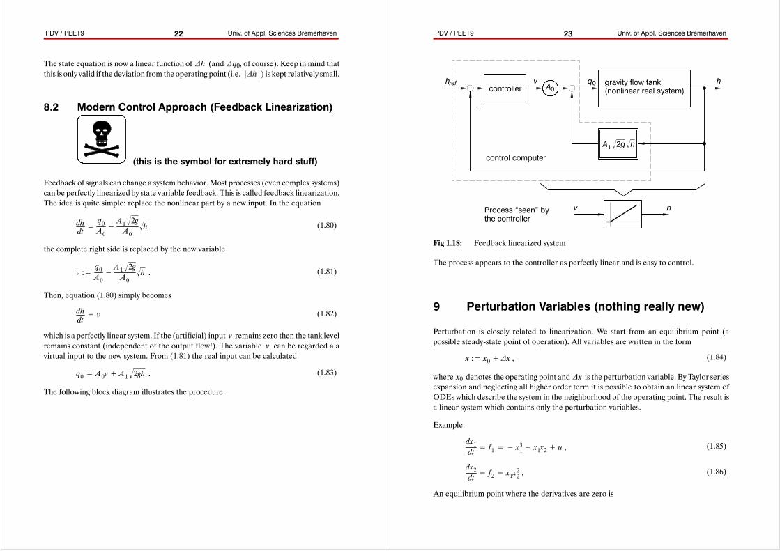
The following block diagram illustrates the procedure.
PDV / PEET9 Univ. of Appl. Sciences Bremerhaven23
gravity flow tank(nonlinear real system)
hq0
A1 2g h
A0controller
---
v
hvProcess “seen” bythe controller
href
control computer
Fig 1.18: Feedback linearized system
The process appears to the controller as perfectly linear and is easy to control.
9 Perturbation Variables (nothing really new)
Perturbation is closely related to linearization. We start from an equilibrium point (apossible steady-state point of operation). All variables are written in the form
x := x0+ ∆x , (1.84)
where x0 denotes the operating point and ∆x is the perturbation variable. By Taylor seriesexpansion and neglecting all higher order term it is possible to obtain an linear system ofODEs which describe the system in the neighborhood of the operating point. The result isa linear system which contains only the perturbation variables.
Example:
dx1dt= f1=− x
31− x1x2+ u , (1.85)
dx2dt= f2= x1x
22 . (1.86)
An equilibrium point where the derivatives are zero is
PDV / PEET9 Univ. of Appl. Sciences Bremerhaven24
x10=3 u0 , x20= 0 . (1.87)
The first order Taylor expansion gives
+∂f1∂ux10,x20,u0
∆u (1.88)
d∆x1dt≈ f1(x10, x20, u0)+
∂f1∂x1x10,x20,u0
∆x1+∂f1∂x1x10,x20,u0
∆x2
It is characteristic for an equilibrium point that f1(x10, x20, u) is zero. Carrying out thederivatives we obtain (note: equation sign is not mathematically correct but used forconvenience)
d∆x1dt=− (3x210+ x20) ∆x1− x10 ∆x2+ ∆u . (1.89)
Applying a first order Taylor expansion to (1.86) gives
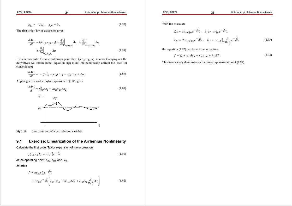
d∆x2dt= x220 ∆x1+ 2x10x20 ∆x2 . (1.90)
t
y∆y
y0
Fig 1.19: Interpretation of a perturbation variable
9.1 Exercise: Linearization of the Arrhenius NonlinearityCalculate the first order Taylor expansion of the expression
f (cA, cB,T)= αcAc2Be− ERT (1.91)
at the operating point cA0, cB0 and T0.
Solution
+ αcB0e− ERT0cB0 ∆cA+ 2cA0 ∆cB+ cA0cB0
ERT20
∆T(1.92)
f ≈ αcA0c2B0e− ERT0
PDV / PEET9 Univ. of Appl. Sciences Bremerhaven25
With the constants
k2 := 2αcA0cB0 e− ERT0 , k3 := αcA0c
2B0ERT20
e−ERT0 . (1.93)
f0 := αcA0c2B0 e− ERT0 , k1 := αc
2B0 e− ERT0 ,
the equation (1.92) can be written in the form
f ≈ f0+ k1 ∆cA+ k2 ∆cB+ k3 ∆T . (1.94)
This form clearly demonstrates the linear approximation of (1.91).
PDV / PEET9 Univ. of Appl. Sciences Bremerhaven26
10 Transfer Function
From conservation of energy and mass the differential equations of a process can bederived. Differential equation are a description in time domain (forODEs the time t is theindependent variable). The analysis of the process behavior and the controller design ismuch easier with a frequency domain representation of the process.
The frequency domain (transfer function) exists, iff the model is linear.
Themain advantageof the frequency domain is that insteadofa setof differential equationsthe process can be described by algebraic equations.
In frequency domain the dynamic model of a process consists of algebraic equations.
10.1 Signal Representation in Frequency Domain(Laplace-Transform)
In the frequency domain all signals are function of the independent variable s. The signalsare the Laplace-transforms of the time domain functions. The Laplace transform is definedas
x(s)= ∞
0
x(t)e−stdt . (2.1)
Note that the Laplace-transform requires functions of the form
x(t)= 0 , t< 0 . (2.2)
Usually no one really carries out the integral (2.1). Instead, tables are used to transformfunctions of time into the s-domain. But (2.1) is not difficult to apply as we see from thetransformation of the step function
σ(t)= 01 t< 0t≥ 0
(2.3)
Since σ(t) is constant from 0 to ∞, the Laplace-transform of (2.3) becomes
σ(s)= ∞
0
e−stdt=− 1s e−st∞
0 =1s . (2.4)
PDV / PEET9 Univ. of Appl. Sciences Bremerhaven27
The Laplace-transform is also denoted as
x(s)= Lx(t) . (2.5)
The inverse is also an integral (over s)
x(t)= 12πjc+j∞
c−j∞
x(s)estds (2.6)
and is denoted as
x(t)= L−1x(s) . (2.7)
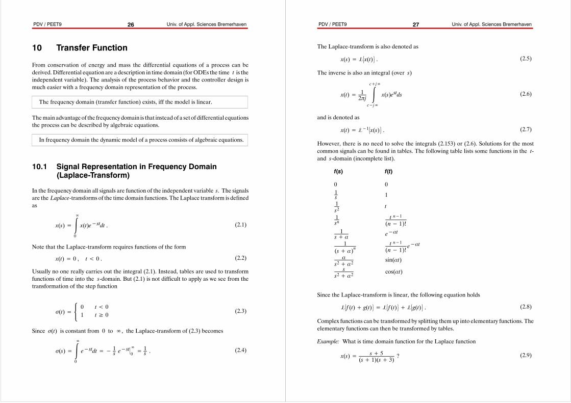
However, there is no need to solve the integrals (2.153) or (2.6). Solutions for the mostcommon signals can be found in tables. The following table lists some functions in the t-and s-domain (incomplete list).
f(s) f(t)
0 01s 11s2
t
1sn
t n−1(n− 1)!
1s+ α e−αt
1(s+ α)n
t n−1(n− 1)!
e−αt
αs2+ α2
sin(αt)
ss2+ α2
cos(αt)
Since the Laplace-transform is linear, the following equation holds
Lf (t)+ g(t) = Lf (t) + Lg(t) . (2.8)
Complex functions can be transformed by splitting them up into elementary functions. Theelementary functions can then be transformed by tables.
Example: What is time domain function for the Laplace function
x(s)= s+ 5(s+ 1)(s+ 3) ?
(2.9)
PDV / PEET9 Univ. of Appl. Sciences Bremerhaven28
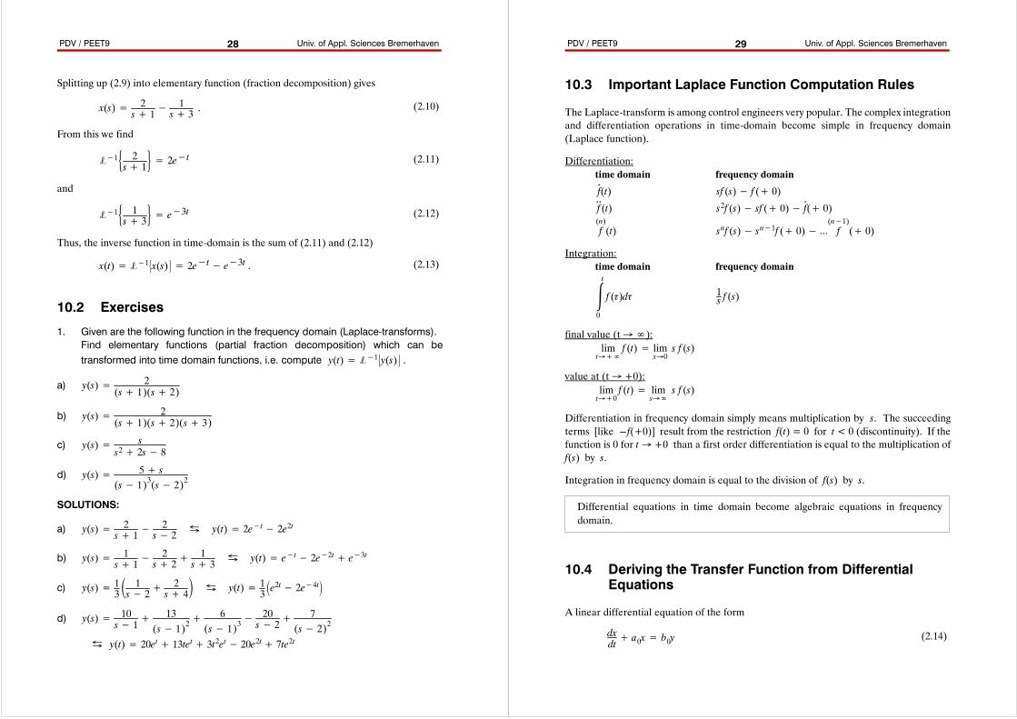
Splitting up (2.9) into elementary function (fraction decomposition) gives
x(s)= 2s+ 1−
1s+ 3 .
(2.10)
From this we find
L−1 2s+ 1 = 2e−t (2.11)
and
L−1 1s+ 3 = e−3t (2.12)
Thus, the inverse function in time-domain is the sum of (2.11) and (2.12)
x(t)= L−1x(s) = 2e−t− e−3t . (2.13)
10.2 Exercises
1. Given are the following function in the frequency domain (Laplace-transforms).Find elementary functions (partial fraction decomposition) which can betransformed into time domain functions, i.e. compute y(t)= L−1y(s) .
a) y(s)= 2(s+ 1)(s+ 2)
b) y(s)= 2(s+ 1)(s+ 2)(s+ 3)
c) y(s)= ss2+ 2s− 8
d) y(s)= 5+ s(s− 1)3(s− 2)2
SOLUTIONS:
a) y(s)= 2s+ 1−
2s− 2 ⇆ y(t)= 2e−t− 2e2t
b) y(s)= 1s+ 1−
2s+ 2+
1s+ 3 ⇆ y(t)= e−t− 2e−2t+ e−3t
c) y(s)= 13 1s− 2+
2s+ 4 ⇆ y(t)= 13
e2t− 2e−4t
d) y(s)= 10s− 1+
13(s− 1)2
+ 6(s− 1)3
− 20s− 2+
7(s− 2)2
⇆ y(t)= 20et+ 13tet+ 3t2et− 20e2t+ 7te2t
PDV / PEET9 Univ. of Appl. Sciences Bremerhaven29
10.3 Important Laplace Function Computation Rules
The Laplace-transform is among control engineers very popular. The complex integrationand differentiation operations in time-domain become simple in frequency domain(Laplace function).
Differentiation:time domain frequency domain
f.(t) sf (s)− f (+ 0)f..(t) s2f (s)− sf (+ 0)− f
.(+ 0)
f(n)(t) snf (s)− sn−1f (+ 0)− f
(n−1)(+ 0)
Integration:time domain frequency domain
t
0
f (τ)dτ 1s f (s)
final value (t→∞):limt→+∞
f (t)= lims→0s f (s)
value at (t→ +0):limt→+0
f (t)= lims→∞
s f (s)
Differentiation in frequency domain simply means multiplication by s. The succeedingterms [like ---f(+0)] result from the restriction f(t) = 0 for t < 0 (discontinuity). If thefunction is 0 for t→ +0 than a first order differentiation is equal to the multiplication off(s) by s.
Integration in frequency domain is equal to the division of f(s) by s.
Differential equations in time domain become algebraic equations in frequencydomain.
10.4 Deriving the Transfer Function from DifferentialEquations
A linear differential equation of the form
dxdt+ a0x= b0y (2.14)
PDV / PEET9 Univ. of Appl. Sciences Bremerhaven30
can be transformed into Laplace domain by using the differentiation rule from section 10.3
sx(s)− x(t=+ 0)+ a0x(s)= b0y(s) . (2.15)
If x(t=+0) = 0 than (2.15) can be solved for x(s)
s+ a0x(s)= b0y(s) , (2.16)
x(s)=b0s+ a0
y(s) . (2.17)
Input and output are related by the algebraic term
G(s) :=b0s+ a0
. (2.18)
G(s) is the transfer function and we write
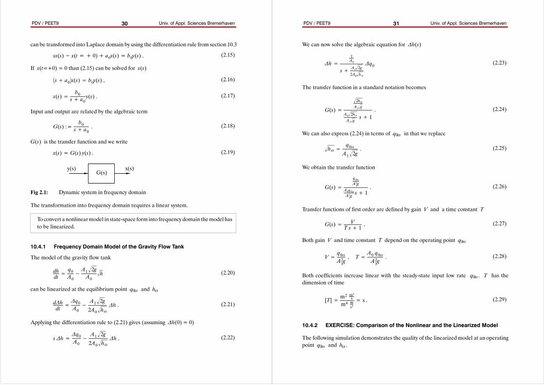
x(s)= G(s) y(s) . (2.19)
y(s) x(s)G(s)
Fig 2.1: Dynamic system in frequency domain
The transformation into frequency domain requires a linear system.
To convert a nonlinearmodel in state-space form into frequency domain themodel hasto be linearized.
10.4.1 Frequency Domain Model of the Gravity Flow Tank
The model of the gravity flow tank
dhdt=q0A0−A1 2gA0
h (2.20)
can be linearized at the equilibrium point q0ss and hss
d∆hdt=∆q0A0−A1 2g
2A0 hss∆h . (2.21)
Applying the differentiation rule to (2.21) gives (assuming ∆h(0) = 0)
s ∆h=∆q0A0−A1 2g
2A0 hss∆h . (2.22)
PDV / PEET9 Univ. of Appl. Sciences Bremerhaven31
We can now solve the algebraic equation for ∆h(s)
∆h=1A0
s+ A1 2g
2A0 hss
∆q0 (2.23)
The transfer function in a standard notation becomes
G(s)=
2hssA1 g
A0 2hssA1 g
s+ 1. (2.24)
We can also express (2.24) in terms of q0ss in that we replace
hss =q0ssA1 2g
. (2.25)
We obtain the transfer function
G(s)=
q0ssA21g
A0q0ssA21gs+ 1
. (2.26)
Transfer functions of first order are defined by gain V and a time constant T
G(s)= VT s+ 1 .
(2.27)
Both gain V and time constant T depend on the operating point q0ss
V=q0ssA21g, T=
A0 q0ssA21g
. (2.28)
Both coefficients increase linear with the steady-state input low rate q0ss . T has thedimension of time
[T]= m2 m3s
m4 ms2= s . (2.29)
10.4.2 EXERCISE: Comparison of the Nonlinear and the Linearized Model
The following simulation demonstrates the quality of the linearized model at an operatingpoint q0ss and hss .
PDV / PEET9 Univ. of Appl. Sciences Bremerhaven32
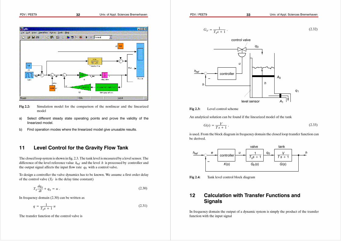
Fig 2.2: Simulation model for the comparison of the nonlinear and the linearizedmodel
a) Select different steady state operating points and prove the validity of thelinearized model.
b) Find operation modes where the linearized model give unusable results.
11 Level Control for the Gravity Flow Tank
The closed loop system is shown in fig. 2.3. The tank level is measuredby a level sensor. Thedifference of the level reference value href and the level h is processed by controller andthe output signal affects the input flow rate q0 with a control valve.
To design a controller the valve dynamics has to be known. We assume a first order delayof the control valve (TV is the delay time constant)
TVdq0dt+ q0= u . (2.30)
In frequency domain (2.30) can be written as
q= 1TVs+ 1
u (2.31)
The transfer function of the control valve is
PDV / PEET9 Univ. of Appl. Sciences Bremerhaven33
GV=1
TVs+ 1. (2.32)
q0
h
q1
A1
A0
control valve
level sensor
controllerhref
h
---
u
Fig 2.3: Level control scheme
An analytical solution can be found if the linearized model of the tank
G(s)= VT s+ 1 .
(2.33)
is used. From the block diagram in frequency domain the closed loop transfer function canbe derived.
controllerhref u q0 hV
T s+ 11
TVs+ 1
G(s)
tank
GV(s)
valve
K(s)
e
---
Fig 2.4: Tank level control block diagram
12 Calculation with Transfer Functions andSignals
In frequency domain the output of a dynamic system is simply the product of the transferfunction with the input signal
PDV / PEET9 Univ. of Appl. Sciences Bremerhaven34
y(s)= G(s) u(s) . (2.34)
It is common practice to drop the argument (s) and write (2.34) as
y= Gu . (2.35)
The following two systems serve as example processes to illustrate various operations ontransfer functions
G1=V1
T1s+ 1, G2=
1T2s. (2.36)
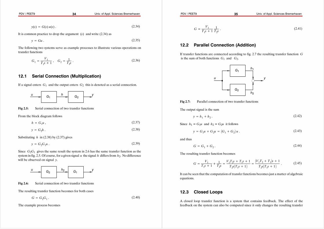
12.1 Serial Connection (Multiplication)
If a signal enters G1 and the output enters G2 this is denoted as a serial connection.
G1 G2u yh
Fig 2.5: Serial connection of two transfer functions
From the block diagram follows
h= G1u , (2.37)
y= G2h . (2.38)
Substituting h in (2.38) by (2.37) gives
y= G2G1u . (2.39)
Since G2G1 gives the same result the system in 2.6 has the same transfer function as thesystem in fig. 2.5. Of course, for a given signal u the signal h differs from h2. Nodifferencewill be observed on signal y.
G1G2u yh2
Fig 2.6: Serial connection of two transfer functions
The resulting transfer function becomes for both cases
G= G2G1 . (2.40)
The example process becomes
PDV / PEET9 Univ. of Appl. Sciences Bremerhaven35
G=V1
T1s+ 11T2s. (2.41)
12.2 Parallel Connection (Addition)
If transfer functions are connected according to fig. 2.7 the resulting transfer function Gis the sum of both functions G1 and G2.
G1
G2
u y
h1
h2
Fig 2.7: Parallel connection of two transfer functions
The output signal is the sum
y= h1+ h2 . (2.42)
Since h1 = G1u and h2 = G2u it follows
y= G1u+G2u= G1+G2 u . (2.43)
and thus
G= G1+G2 . (2.44)
The resulting transfer function becomes
G=V1
T1s+ 1+ 1T2s=V1T2s+ T1s+ 1T2sT1s+ 1
=V1T2+ T1s+ 1T2sT1s+ 1
. (2.45)
It can be seen that the computation of transfer functions becomes just amatter of algebraicequations.
12.3 Closed Loops
A closed loop transfer function is a system that contains feedback. The effect of thefeedback on the system can also be computed since it only changes the resulting transfer
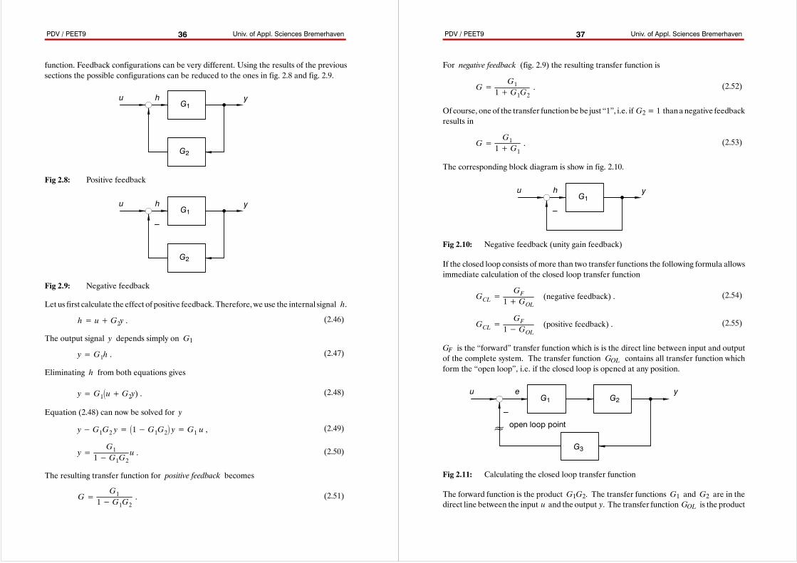
PDV / PEET9 Univ. of Appl. Sciences Bremerhaven36
function. Feedback configurations can be very different. Using the results of the previoussections the possible configurations can be reduced to the ones in fig. 2.8 and fig. 2.9.
G1
G2
u h y
Fig 2.8: Positive feedback
G1
G2
u h y
---
Fig 2.9: Negative feedback
Let us first calculate the effect of positive feedback. Therefore, we use the internal signal h.
h= u+G2y . (2.46)
The output signal y depends simply on G1
y= G1h . (2.47)
Eliminating h from both equations gives
y= G1u+G2y) . (2.48)
Equation (2.48) can now be solved for y
y−G1G2 y= 1−G1G2 y= G1 u , (2.49)
y=G1
1−G1G2u . (2.50)
The resulting transfer function for positive feedback becomes
G=G1
1−G1G2. (2.51)
PDV / PEET9 Univ. of Appl. Sciences Bremerhaven37
For negative feedback (fig. 2.9) the resulting transfer function is
G=G1
1+G1G2. (2.52)
Of course, one of the transfer functionbe be just “1”, i.e. if G2 = 1 thana negative feedbackresults in
G=G11+G1
. (2.53)
The corresponding block diagram is show in fig. 2.10.
G1u h y
---
Fig 2.10: Negative feedback (unity gain feedback)
If the closed loop consists of more than two transfer functions the following formula allowsimmediate calculation of the closed loop transfer function
GCL=GF
1+GOL(negative feedback) . (2.54)
GCL=GF
1−GOL(positive feedback) . (2.55)
GF is the “forward” transfer function which is is the direct line between input and outputof the complete system. The transfer function GOL contains all transfer function whichform the “open loop”, i.e. if the closed loop is opened at any position.
u yeG1 G2
G3
---
≈ open loop point
Fig 2.11: Calculating the closed loop transfer function
The forward function is the product G1G2. The transfer functions G1 and G2 are in thedirect line between the input u and the output y. The transfer function GOL is the product
PDV / PEET9 Univ. of Appl. Sciences Bremerhaven38
of all open loop functions when the closed loop is opened (for instance at the markedposition) GOL = G1G2G3. Since we have negative feedback (most common for controlsystems) the closed loop transfer function becomes
GCL=G1G2
1+G1G2G3. (2.56)
Of course, the calculation can be carried out in several steps, for instance
e= u−G1G2G3e , (2.57)
y= G1G2e . (2.58)
From (2.57) follows
e= 11+G1G2G3
u (2.59)
and with (2.58) we arrive at the same result (2.56).
The resulting transfer function (2.56) looks complicated but it can be often simplified. Theexample in fig. 2.9 gives the transfer function
GCL=G1
1+G1G2=
V1T1s+1
1+ V1T1s+1
1T2s
. (2.60)
The complicated formof (2.60) becomesmuch simpler whenNumerator andDenominatorare multiplied by (T1s+1)T2s
GCL= V1T2s
T1s+ 1T2s+ V1. (2.61)
it can be easily seen that the closed loop system has a completely different structure thanthe open loop transfer function.
If the open loop transfer function is real rational than the closed loop transfer functionis real rational too.
13 Elementary Transfer Functions
Every complex transfer function consists of elementary functions. Following is a list ofelementary functions. The symbol is derived from the step response of the system.
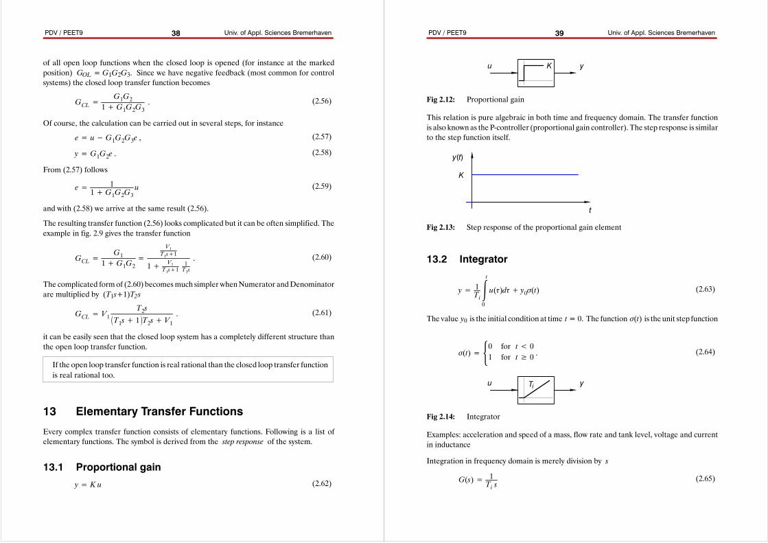
13.1 Proportional gainy= K u (2.62)
PDV / PEET9 Univ. of Appl. Sciences Bremerhaven39
u yK
Fig 2.12: Proportional gain
This relation is pure algebraic in both time and frequency domain. The transfer functionis also knownas the P-controller (proportional gain controller). The step response is similarto the step function itself.
t
y(t)
K
Fig 2.13: Step response of the proportional gain element
13.2 Integrator
y= 1Tit
0
u(τ)dτ+ y0σ(t) (2.63)
The value y0 is the initial condition at time t = 0. The function σ(t) is theunit step function
σ(t)= 0 for t< 01 for t≥ 0 .
(2.64)
u yTi
Fig 2.14: Integrator
Examples: acceleration and speed of a mass, flow rate and tank level, voltage and currentin inductance
Integration in frequency domain is merely division by s
G(s)= 1Ti s
(2.65)
PDV / PEET9 Univ. of Appl. Sciences Bremerhaven40
The step response is the product of the transfer function and σ(s)
y(s)= F(s)σ(s)= 1Tis1s =
1Tis2
. (2.66)
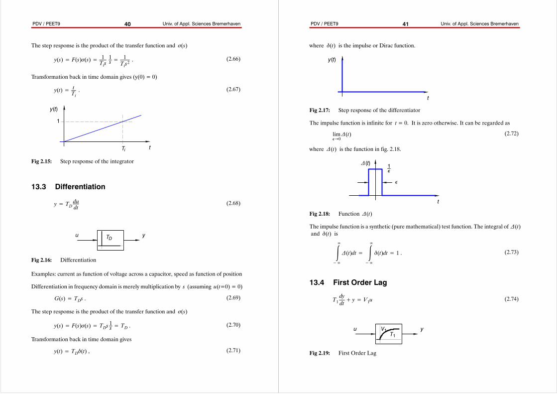
Transformation back in time domain gives (y(0) = 0)
y(t)= tTi. (2.67)
t
y(t)
Ti
1
Fig 2.15: Step response of the integrator
13.3 Differentiation
y= TDdudt
(2.68)
u yTD
Fig 2.16: Differentiation
Examples: current as function of voltage across a capacitor, speed as function of position
Differentiation in frequency domain is merely multiplication by s (assuming u(t=0) = 0)
G(s)= TDs . (2.69)
The step response is the product of the transfer function and σ(s)
y(s)= F(s)σ(s)= TDs1s = TD . (2.70)
Transformation back in time domain gives
y(t)= TDδ(t) , (2.71)
PDV / PEET9 Univ. of Appl. Sciences Bremerhaven41
where δ(t) is the impulse or Dirac function.
t
y(t)
Fig 2.17: Step response of the differentiator
The impulse function is infinite for t = 0. It is zero otherwise. It can be regarded as
limÁ→0∆(t) (2.72)
where ∆(t) is the function in fig. 2.18.
t
∆(t)
Á
1Á
Fig 2.18: Function ∆(t)
The impulse function is a synthetic (pure mathematical) test function. The integral of ∆(t)and δ(t) is
∞
−∞
∆(t)dt= ∞
−∞
δ(t)dt= 1 . (2.73)
13.4 First Order Lag
T1dydt+ y= V1u (2.74)
u yT1
V1
Fig 2.19: First Order Lag
PDV / PEET9 Univ. of Appl. Sciences Bremerhaven42
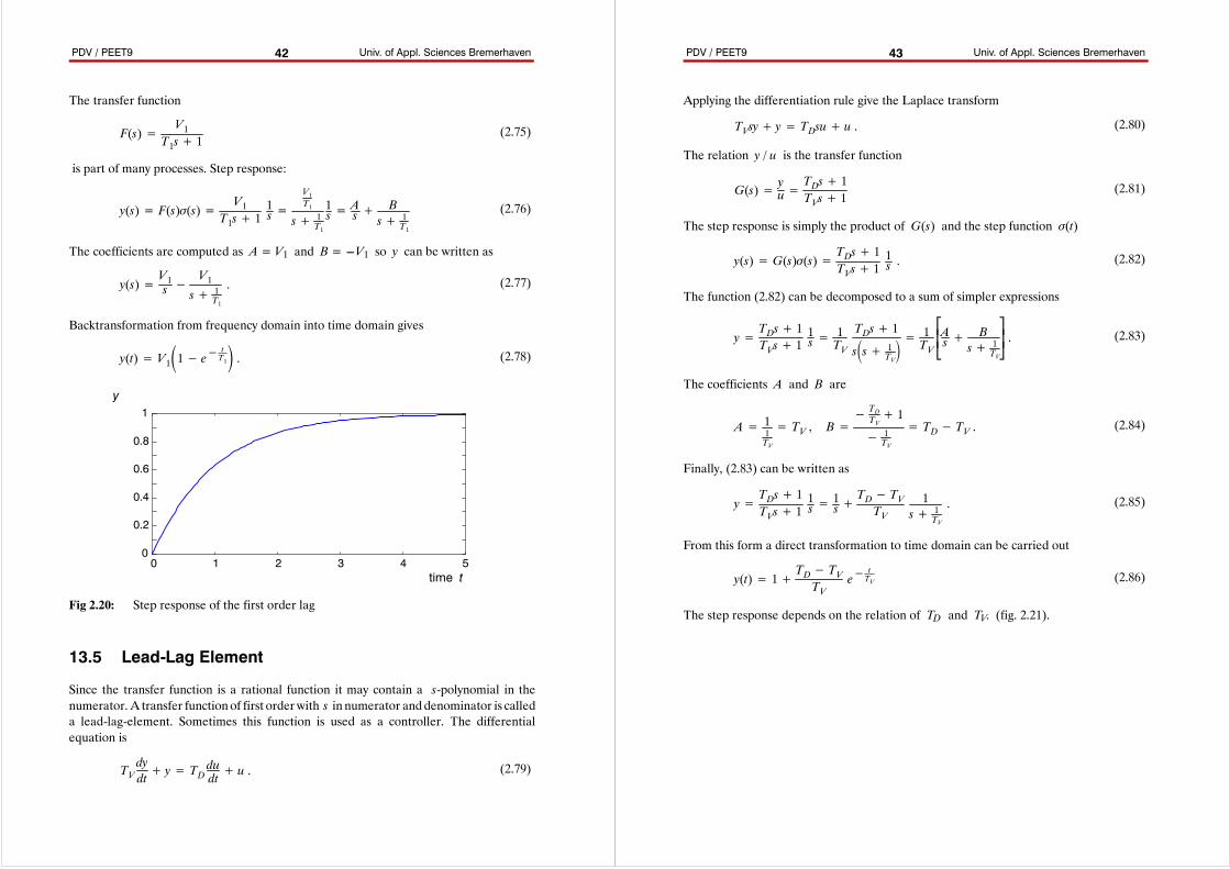
The transfer function
F(s)=V1
T1s+ 1(2.75)
is part of many processes. Step response:
y(s)= F(s)σ(s)=V1
T1s+ 11s =
V1T1
s+ 1T1
1s =As +
Bs+ 1
T1
(2.76)
The coefficients are computed as A = V1 and B = ---V1 so y can be written as
y(s)=V1s −
V1s+ 1
T1
. (2.77)
Backtransformation from frequency domain into time domain gives
y(t)= V11− e− tT1 . (2.78)
0
0.2
0.4
0.6
0.8
1
0 1 2 3 4 5time t
y
Fig 2.20: Step response of the first order lag
13.5 Lead-Lag Element
Since the transfer function is a rational function it may contain a s-polynomial in thenumerator. A transfer functionof first order with s in numerator anddenominator is calleda lead-lag-element. Sometimes this function is used as a controller. The differentialequation is
TVdydt+ y= TD
dudt+ u . (2.79)
PDV / PEET9 Univ. of Appl. Sciences Bremerhaven43
Applying the differentiation rule give the Laplace transform
TVsy+ y= TDsu+ u . (2.80)
The relation y / u is the transfer function
G(s)= yu=TDs+ 1TVs+ 1
(2.81)
The step response is simply the product of G(s) and the step function σ(t)
y(s)= G(s)σ(s)=TDs+ 1TVs+ 1
1s . (2.82)
The function (2.82) can be decomposed to a sum of simpler expressions
y=TDs+ 1TVs+ 1
1s =
1TV
TDs+ 1
ss+ 1TV =
1TVAs +
Bs+ 1
TV
. (2.83)
The coefficients A and B are
A= 11TV
= TV , B=− TDTV+ 1
− 1TV
= TD− TV . (2.84)
Finally, (2.83) can be written as
y=TDs+ 1TVs+ 1
1s =1s+TD− TVTV
1s+ 1
TV
. (2.85)
From this form a direct transformation to time domain can be carried out
y(t)= 1+TD− TVTV
e−tTV (2.86)
The step response depends on the relation of TD and TV. (fig. 2.21).
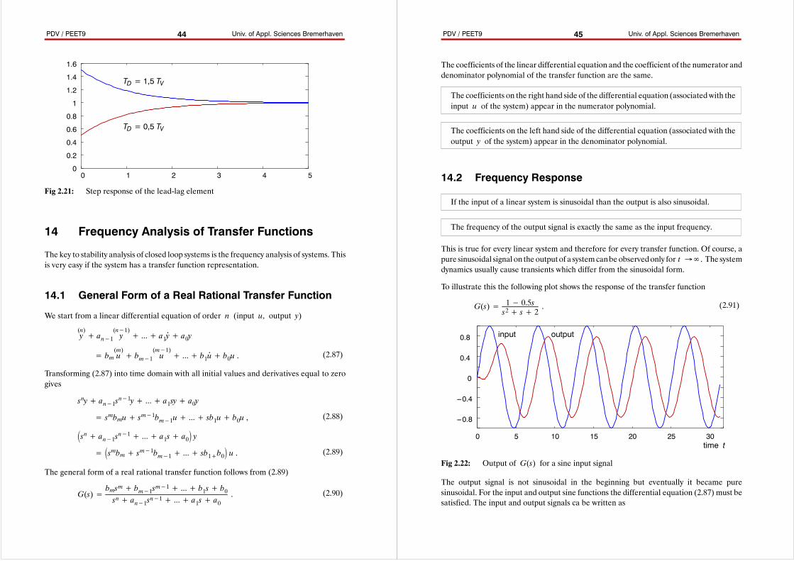
PDV / PEET9 Univ. of Appl. Sciences Bremerhaven44
0
0.2
0.4
0.6
0.8
1
1.2
1.4
1.6
0 1 2 3 4 5
TD = 1,5 TV
TD = 0,5 TV
Fig 2.21: Step response of the lead-lag element
14 Frequency Analysis of Transfer Functions
The key to stability analysis of closed loop systems is the frequency analysis of systems. Thisis very easy if the system has a transfer function representation.
14.1 General Form of a Real Rational Transfer Function
We start from a linear differential equation of order n (input u, output y)
= bm u(m)+ bm−1 u
(m−1)+ + b1u
. + b0u . (2.87)
y(n)+ an−1 y
(n−1)+ + a1y
. + a0y
Transforming (2.87) into time domain with all initial values and derivatives equal to zerogives
= smbmu+ sm−1bm−1u+ + sb1u+ b0u , (2.88)
sny+ an−1sn−1y+ + a1sy+ a0y
= smbm+ sm−1bm−1+ + sb1+b0 u . (2.89)
sn+ an−1sn−1+ + a1s+ a0 y
The general form of a real rational transfer function follows from (2.89)
G(s)=bmsm+ bm−1sm−1+ + b1s+ b0sn+ an−1sn−1+ + a1s+ a0
. (2.90)
PDV / PEET9 Univ. of Appl. Sciences Bremerhaven45
The coefficients of the linear differential equation and the coefficient of the numerator anddenominator polynomial of the transfer function are the same.
The coefficients on the right hand side of the differential equation (associatedwith theinput u of the system) appear in the numerator polynomial.
The coefficients on the left hand side of the differential equation (associated with theoutput y of the system) appear in the denominator polynomial.
14.2 Frequency Response
If the input of a linear system is sinusoidal than the output is also sinusoidal.
The frequency of the output signal is exactly the same as the input frequency.
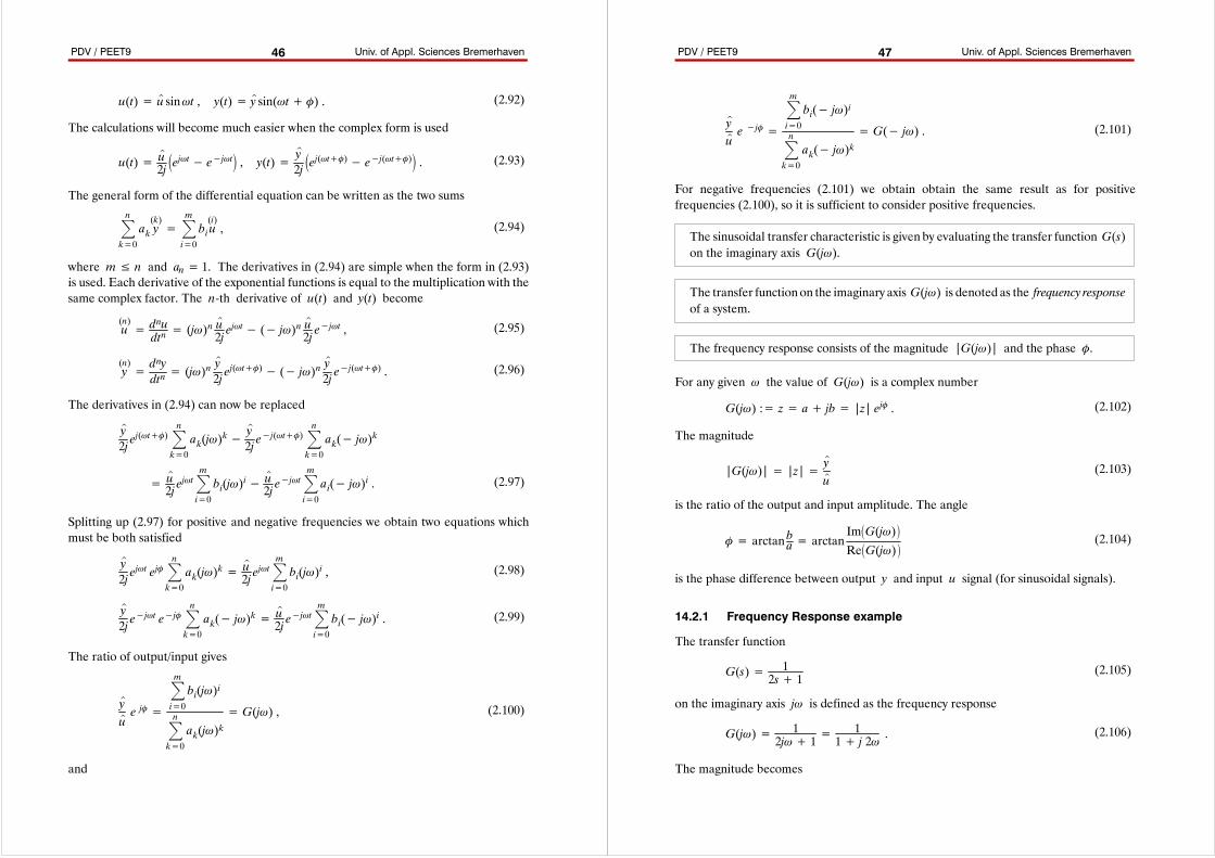
This is true for every linear system and therefore for every transfer function. Of course, apure sinusoidal signal on the outputof a systemcanbe observedonly for t →∞. The systemdynamics usually cause transients which differ from the sinusoidal form.
To illustrate this the following plot shows the response of the transfer function
G(s)= 1− 0.5ss2+ s+ 2
. (2.91)
0 5 10 15 20 25 30
---0.8
---0.4
0
0.4
0.8
time t
input output
Fig 2.22: Output of G(s) for a sine input signal
The output signal is not sinusoidal in the beginning but eventually it became puresinusoidal. For the input and output sine functions the differential equation (2.87) must besatisfied. The input and output signals ca be written as
PDV / PEET9 Univ. of Appl. Sciences Bremerhaven46
u(t)= u^sinωt , y(t)= y^sin(ωt+ Ô) . (2.92)
The calculations will become much easier when the complex form is used
u(t)= u^
2jejωt− e−jωt , y(t)= y
^
2jej(ωt+Ô)− e−j(ωt+Ô) . (2.93)
The general form of the differential equation can be written as the two sums
nk=0ak y(k)=mi=0biu(i), (2.94)
where m≤ n and an = 1. The derivatives in (2.94) are simple when the form in (2.93)is used. Each derivative of the exponential functions is equal to the multiplication with thesame complex factor. The n-th derivative of u(t) and y(t) become
u(n)= d
nudtn= (jω)n u
^
2j ejωt− (− jω)n u
^
2j e−jωt , (2.95)
y(n)=dnydtn= (jω)n
y^
2j ej(ωt+Ô)− (− jω)n
y^
2j e−j(ωt+Ô) . (2.96)
The derivatives in (2.94) can now be replaced
= u^
2j ejωtmi=0bi(jω)
i− u^
2j e−jωtm
i=0ai(− jω)i . (2.97)
y^
2j ej(ωt+Ô)n
k=0ak(jω)
k−y^
2j e−j(ωt+Ô)n
k=0ak(− jω)
k
Splitting up (2.97) for positive and negative frequencies we obtain two equations whichmust be both satisfied
y^
2j ejωt ejÔn
k=0ak(jω)
k= u^
2j ejωtmi=0bi(jω)
i , (2.98)
y^
2j e−jωt e−jÔn
k=0ak(− jω)
k= u^
2j e−jωtm
i=0bi(− jω)i . (2.99)
The ratio of output/input gives
y^
u^e jÔ=
mi=0bi(jω)i
nk=0ak(jω)k
= G(jω) , (2.100)
and
PDV / PEET9 Univ. of Appl. Sciences Bremerhaven47
y^
u^e −jÔ=
mi=0bi(− jω)i
nk=0ak(− jω)k
= G(− jω) . (2.101)
For negative frequencies (2.101) we obtain obtain the same result as for positivefrequencies (2.100), so it is sufficient to consider positive frequencies.
The sinusoidal transfer characteristic is given by evaluating the transfer function G(s)on the imaginary axis G(jω).
The transfer functionon the imaginary axis G(jω) is denoted as the frequency responseof a system.
The frequency response consists of the magnitude |G(jω)| and the phase Ô.
For any given ω the value of G(jω) is a complex number
G(jω) := z= a+ jb= |z| ejÔ . (2.102)
The magnitude
|G(jω)|= |z|=y^
u^(2.103)
is the ratio of the output and input amplitude. The angle
Ô= arctan ba= arctanImG(jω)ReG(jω)
(2.104)
is the phase difference between output y and input u signal (for sinusoidal signals).
14.2.1 Frequency Response example
The transfer function
G(s)= 12s+ 1
(2.105)
on the imaginary axis jω is defined as the frequency response
G(jω)= 12jω+ 1=
11+ j 2ω .
(2.106)
The magnitude becomes
PDV / PEET9 Univ. of Appl. Sciences Bremerhaven48
|G(jω)|= 14ω2+ 1 . (2.107)
The calculation of the phase is more complicated. We can multiply (2.106) by the complexconjugate of the denominator
G(jω)= 11+ j 2ω
1− j 2ω1− j 2ω=
1− j 2ω1+ 4ω2
. (2.108)
The real and imaginary parts are
ReG(jω) = 11+ 4ω2
, ImG(jω) = − j 2ω1+ 4ω2
. (2.109)
Therefore the angle becomes
Ô= arctanImG(jω)ReG(jω)
= arctan− 2ω1=− arctan 2ω . (2.110)
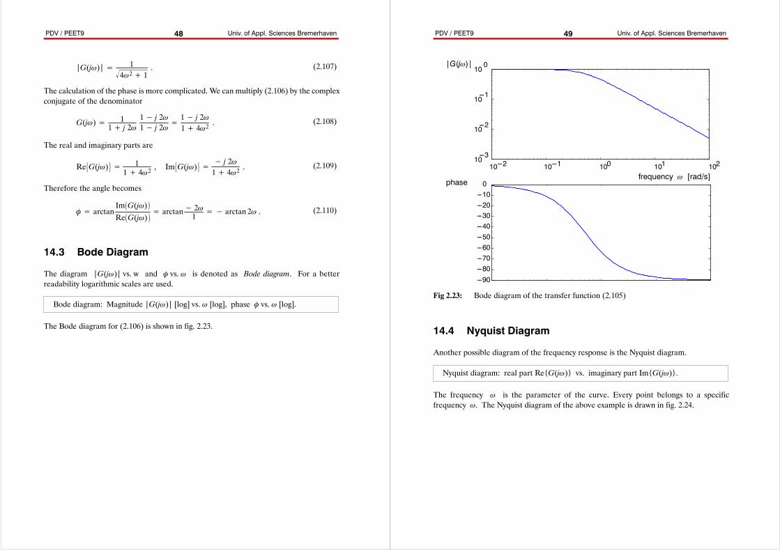
14.3 Bode Diagram
The diagram |G(jω)| vs. w and Ô vs. ω is denoted as Bode diagram. For a betterreadability logarithmic scales are used.
Bode diagram: Magnitude |G(jω)| [log] vs. ω [log], phase Ô vs. ω [log].
The Bode diagram for (2.106) is shown in fig. 2.23.
PDV / PEET9 Univ. of Appl. Sciences Bremerhaven49
---90---80---70---60---50---40---30---20---100
10---2 10---1 100 101 10210---3
10---2
10---1
100
frequency ω [rad/s]phase
|G(jω)|
Fig 2.23: Bode diagram of the transfer function (2.105)
14.4 Nyquist Diagram
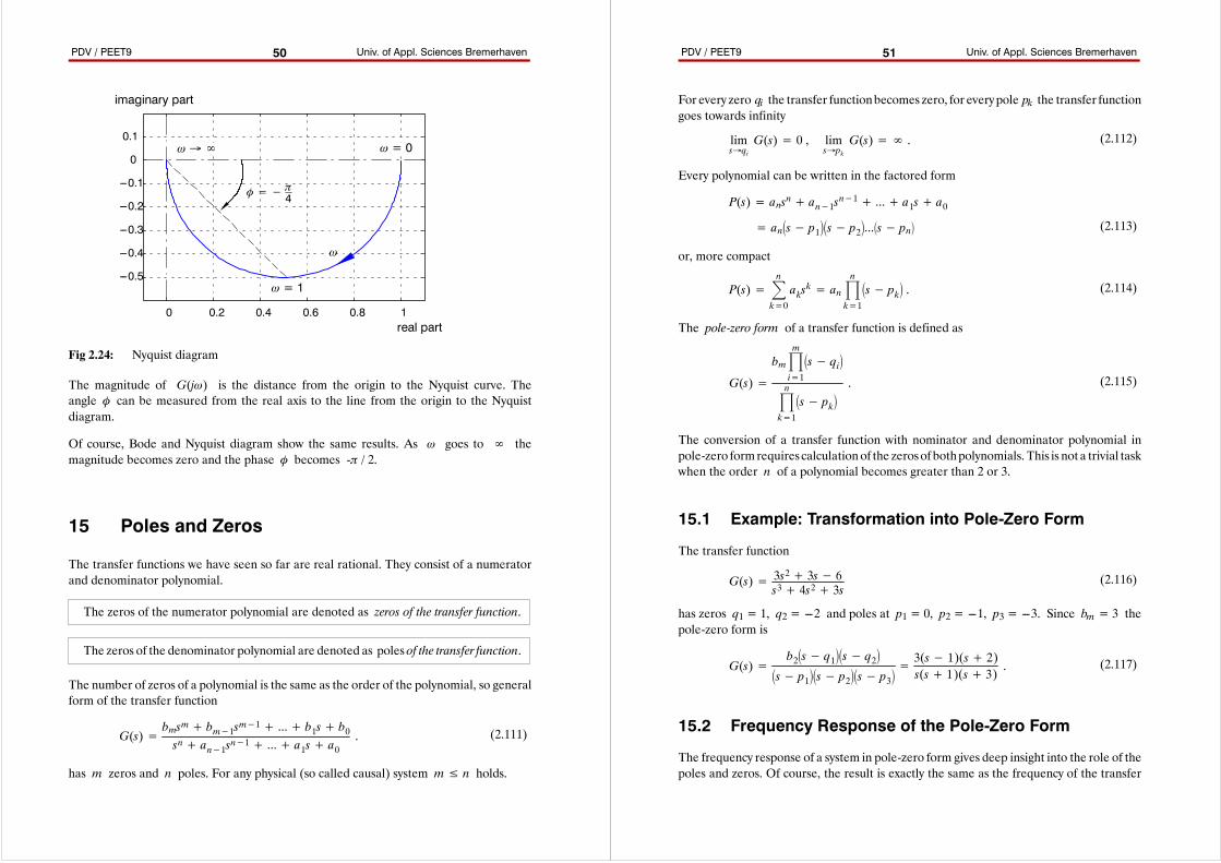
Another possible diagram of the frequency response is the Nyquist diagram.
Nyquist diagram: real part Re{G(jω)} vs. imaginary part Im{G(jω)}.
The frequency ω is the parameter of the curve. Every point belongs to a specificfrequency ω. The Nyquist diagram of the above example is drawn in fig. 2.24.
PDV / PEET9 Univ. of Appl. Sciences Bremerhaven50
0 0.2 0.4 0.6 0.8 1
---0.5
---0.4
---0.3
---0.2
---0.1
0
0.1
real part
imaginary part
ω = 0
ω = 1
ω→∞
Ô=− π4
ω
Fig 2.24: Nyquist diagram
The magnitude of G(jω) is the distance from the origin to the Nyquist curve. Theangle Ô can be measured from the real axis to the line from the origin to the Nyquistdiagram.
Of course, Bode and Nyquist diagram show the same results. As ω goes to ∞ themagnitude becomes zero and the phase Ô becomes -π / 2.
15 Poles and Zeros
The transfer functions we have seen so far are real rational. They consist of a numeratorand denominator polynomial.
The zeros of the numerator polynomial are denoted as zeros of the transfer function.
The zeros of the denominator polynomial are denoted as poles of the transfer function.
The number of zeros of a polynomial is the same as the order of the polynomial, so generalform of the transfer function
G(s)=bmsm+ bm−1sm−1+ + b1s+ b0sn+ an−1sn−1+ + a1s+ a0
. (2.111)
has m zeros and n poles. For any physical (so called causal) system m≤ n holds.
PDV / PEET9 Univ. of Appl. Sciences Bremerhaven51
For every zero qi the transfer functionbecomes zero, for everypole pk the transfer functiongoes towards infinity
lims→qiG(s)= 0 , lim
s→pkG(s)=∞ . (2.112)
Every polynomial can be written in the factored form
= ans− p1s− p2s− pn (2.113)
P(s)= ansn+ an−1sn−1+ + a1s+ a0
or, more compact
P(s)= nk=0aksk= an
n
k=1
s− pk . (2.114)
The pole-zero form of a transfer function is defined as
G(s)=
bmm
i=1
s− qi
nk=1
s− pk. (2.115)
The conversion of a transfer function with nominator and denominator polynomial inpole-zero formrequires calculationof the zerosof bothpolynomials. This is nota trivial taskwhen the order n of a polynomial becomes greater than 2 or 3.
15.1 Example: Transformation into Pole-Zero Form
The transfer function
G(s)= 3s2+ 3s− 6
s3+ 4s2+ 3s(2.116)
has zeros q1 = 1, q2 = ---2 and poles at p1 = 0, p2 = ---1, p3 = ---3. Since bm = 3 thepole-zero form is
G(s)=b2s− q1s− q2
s− p1s− p2s− p3=3(s− 1)(s+ 2)s(s+ 1)(s+ 3)
. (2.117)
15.2 Frequency Response of the Pole-Zero Form
The frequency response of a system in pole-zero form gives deep insight into the role of thepoles and zeros. Of course, the result is exactly the same as the frequency of the transfer
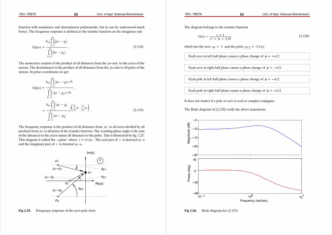
PDV / PEET9 Univ. of Appl. Sciences Bremerhaven52
function with nominator and denominator polynomials, but in can be understood muchbetter. The frequency response is defined as the transfer function on the imaginary axis
G(jω)=
bmm
i=1
jω− qi
nk=1
jω− pk. (2.118)
The numerator consists of the product of all distances from the jω-axis to the zeros of thesystem. The denominator is the product of all distances from the jω-axis to all poles of thesystem. In polar coordinates we get
=
bmm
i=1
jω− qi
nk=1
jω− pkejmi=1
Ôi−n
k=1
Ôk. (2.119)
G(jω)=
bmm
i=1
jω− qi e jÔi
nk=1
jω− pk e jÔk.
The frequency response is the product of all distances from jω to all zeros divided by allproducts from jω to all poles of the transfer function. The resulting phase angle is the sumof the distances to the zeros minus all distances to the poles. This is illustrated by fig. 2.25.This diagram is called the s plane where s = σ+jω. The real part of s is denoted as σand the imaginary part of s is denoted as ω.
s
jω
Im(s)
Re(s)q1
p1
p2
jω---p1
jω---q1
jω---p2
Ôp1
Ôq1
Ôp2
Fig 2.25: Frequency response of the zero-pole form
PDV / PEET9 Univ. of Appl. Sciences Bremerhaven53
The diagram belongs to the transfer function
G(s)= s+ 1s2+ 3s+ 3.25
(2.120)
which has the zero q1 = -1 and the poles p1/2 = -1,5±j.
Each zero in left half plane causes a phase change of Ô = +π/2.
Each zero in right half plane causes a phase change of Ô = ---π/2.
Each pole in left half plane causes a phase change of Ô = ---π/2.
Each pole in right half plane causes a phase change of Ô = +π/2.
It does not matter if a pole or zero is real or complex conjugate.
The Bode diagram of (2.120) verify the above statements.
Frequency (rad/sec)
Phase(deg)
Magnitude(dB)
---25
---20
---15
---10
---5
10---1 100 101
---90
---45
0
45
Fig 2.26: Bode diagram for (2.153)
PDV / PEET9 Univ. of Appl. Sciences Bremerhaven54
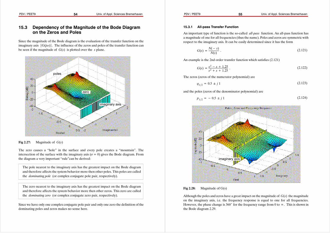
15.3 Dependency of the Magnitude of the Bode Diagramon the Zeros and Poles
Since the magnitude of the Bode diagram is the evaluation of the transfer function on theimaginary axis |G(jω)|. The influence of the zeros and poles of the transfer function canbe seen if the magnitude of G(s) is plotted over the s plane.
zero
poles
imaginary axis
Fig 2.27: Magnitude of G(s)
The zero causes a “hole” in the surface and every pole creates a “mountain”. Theintersection of the surface with the imaginary axis (σ = 0) gives the Bode diagram. Fromthe diagram a very important “rule”can be derived:
The pole nearest to the imaginary axis has the greatest impact on the Bode diagramand therefore affects the system behavior more then other poles. This poles are calledthe dominating pole (or complex conjugate pole pair, respectively).
The zero nearest to the imaginary axis has the greatest impact on the Bode diagramand therefore affects the system behavior more then other zeros. This zero are calledthe dominating zero (or complex conjugate zero pair, respectively).
Since we have only one complex conjugate pole pair and only one zero the definition of thedominating poles and zeros makes no sense here.
PDV / PEET9 Univ. of Appl. Sciences Bremerhaven55
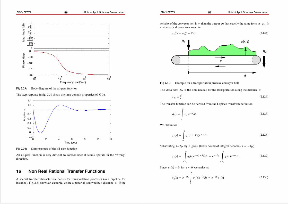
15.3.1 All-pass Transfer Function
An important type of function is the so-called all-pass function. An all-pass function hasa magnitude of one for all frequencies (thus the name). Poles and zeros are symmetric withrespect to the imaginary axis. It can be easily determined since it has the form
G(s)=N(− s)N(s)
. (2.121)
An example is the 2nd order transfer function which satisfies (2.121)
G(s)= s2− s+ 1.25s2+ s+ 1.25
. (2.122)
The zeros (zeros of the numerator polynomial) are
q1∕2= 0.5 j 1 (2.123)
and the poles (zeros of the denominator polynomial) are
p1∕2=− 0.5 j 1 (2.124)
imaginary axis
Fig 2.28: Magnitude of G(s)
Although the poles and zeros have a great impact on themagnitude of G(s) themagnitudeon the imaginary axis, i.e. the frequency response is equal to one for all frequencies.However, the phase change is 360˚ for the frequency range from 0 to∞. This is shown inthe Bode diagram 2.29.
PDV / PEET9 Univ. of Appl. Sciences Bremerhaven56
Frequency (rad/sec)
Phase(deg)
Magnitude(dB)
---1---0.8---0.6---0.4---0.200.20.40.60.81
10---1
100
101
102
---360
---270
---180
---90
0
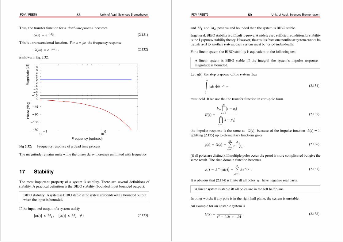
Fig 2.29: Bode diagram of the all-pass function
The step response in fig. 2.30 shows the time domain properties of G(s).
Time (sec)
Amplitude
0 2 4 6 8 10 12---0.2
0
0.2
0.4
0.6
0.8
1
1.2
1.4
Fig 2.30: Step response of the all-pass function
An all-pass function is very difficult to control since it seems operate in the “wrong”direction.
16 Non Real Rational Transfer Functions
A special transfer characteristic occurs for transportation processes (in a pipeline forinstance). Fig. 2.31 shows an example, where a material is moved by a distance d. If the
PDV / PEET9 Univ. of Appl. Sciences Bremerhaven57
velocity of the conveyor belt is v than the output q2 has exactly the same form as q1. Inmathematical terms we can write
q2(t)= q1(t− TD) . (2.125)
v
q1
q2
d
c(x, t)
Fig 2.31: Example for a transportation process: conveyor belt
The dead time TD is the time needed for the transportation along the distance d
TD=dv . (2.126)
The transfer function can be derived from the Laplace transform definition
x(s)= ∞
0
x(t)e−stdt . (2.127)
We obtain for
q2(s)= ∞
0
q1(t− TD)e−stdt . (2.128)
Substituting t---TD by τ gives (lower bound of integral becomes τ = ---TD)
q2(s)= ∞
−TD
q1(τ)e−s(τ+TD)dτ= e−sTD
∞
−TD
q1(τ)e−sτdτ . (2.129)
Since q1(τ) = 0 for τ < 0 we arrive at
q2(s)= e−sTD
∞
0
q1(τ)e−sτdτ= e−sT q1(s) . (2.130)
PDV / PEET9 Univ. of Appl. Sciences Bremerhaven58
Thus, the transfer function for a dead time process becomes
G(s)= e−sTD . (2.131)
This is a transcendental function. For s = jω the frequency response
G(jω)= e−jωTD . (2.132)
is shown in fig. 2.32.
Frequency (rad/sec)
Phase(deg)
Magnitude(dB)
---10---8---6---4---202468
10---1
100---180
---135
---90
---45
0
Fig 2.32: Frequency response of a dead time process
The magnitude remains unity while the phase delay increases unlimited with frequency.
17 Stability
The most important property of a system is stability. There are several definitions ofstability. A practical definition is the BIBO stability (bounded input bounded output):
BIBO stability: A system is BIBO stable if the system responds with a bounded outputwhen the input is bounded.
If the input and output of a system satisfy
|u(t)|≤ M1 , |y(t)|≤ M2 ∀ t (2.133)
PDV / PEET9 Univ. of Appl. Sciences Bremerhaven59
and M1 and M2 positive and bounded than the system is BIBO stable.
Ingeneral, BIBOstability is difficult to prove.Awidelyused sufficient condition for stabilityis the Lyapunov stability theory. However, the results from one nonlinear system cannot betransferred to another system; each system must be tested individually.
For a linear system the BIBO stability is equivalent to the following test:
A linear system is BIBO stable iff the integral the system’s impulse responsemagnitude is bounded.
Let g(t) the step response of the system then
∞
0
|g(t)|dt<∞ (2.134)
must hold. If we use the the transfer function in zero-pole form
G(s)=
bmm
i=1
s− qi
nk=1
s− pk(2.135)
the impulse response is the same as G(s) because of the impulse function δ(s) = 1.Splitting (2.135) up to elementary functions gives
g(s)= G(s)= nk=1
Aks− pk
(2.136)
(if all poles are distinct). If multiple poles occur the proof is more complicated but give thesame result. The time domain function becomes
g(t)= L−1g(s) = nk=1Ae−pk t . (2.137)
It is obvious that (2.134) is finite iff all poles pk have negative real parts.
A linear system is stable iff all poles are in the left half plane.
In other words: if any pole is in the right half plane, the system is unstable.
An example for an unstable system is
G(s)= 1s2− 0.2s+ 1.01
. (2.138)
PDV / PEET9 Univ. of Appl. Sciences Bremerhaven60
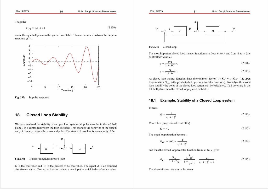
The poles
p1∕2= 0.1 j 1 (2.139)
are in the right half plane so the system is unstable. The can be seen also from the impulseresponse g(t).
Time (sec)
Amplitude
0 5 10 15 20 25
---10
---8
---6
---4
---2
0
2
4
6
8
Fig 2.33: Impulse response
18 Closed Loop Stability
We have analyzed the stability of an open loop system (all poles must be in the left halfplane). In a controlled system the loop is closed. This changes the behavior of the systemand, of course, changes the zeros and poles. The standard problem is shown in fig. 2.34.
e u
d
yK G
Fig 2.34: Transfer functions in open loop
K is the controller and G is the process to be controlled. The signal d is an assumeddisturbance signal. Closing the loop introduces a new input w which is the reference value.
PDV / PEET9 Univ. of Appl. Sciences Bremerhaven61
e u
d
yK G
w
---
Fig 2.35: Closed loop
The most important closed loop transfer functions are from w to y and from d to y (thecontrolled variable)
y= KG1+ KGw ,
(2.140)
y= G1+ KGd .
(2.141)
All closed loop transfer functions have the common “factor” 1+KG = 1+GOL (the openloop function GOL is the product of all open loop transfer functions). To analyze the closedloop stability the poles of the closed loop system can be calculated. If all poles are in theleft half plane than the closed loop system is stable.
18.1 Example: Stability of a Closed Loop system
Process
G= 1(s+ 1)3
(2.142)
Controller (proportional controller)
K= 4 . (2.143)
The open loop function becomes
GOL= KG=4
(s+ 1)3(2.144)
and thus the closed loop transfer function from w to y gives
GCL=GOL1+GOL
=
4(s+1)3
1+ 4(s+1)3
= 4(s+ 1)3+ 4
. (2.145)
The denominator polynomial becomes
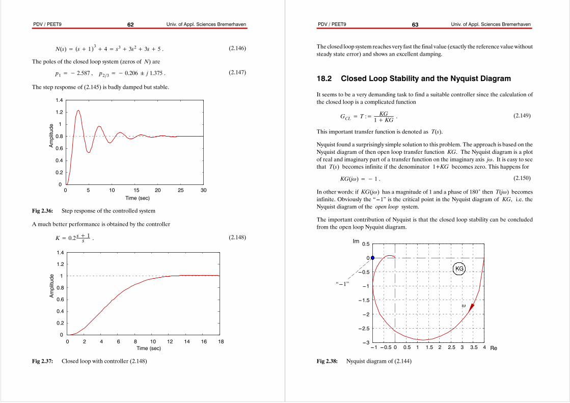
PDV / PEET9 Univ. of Appl. Sciences Bremerhaven62
N(s)= (s+ 1)3+ 4= s3+ 3s2+ 3s+ 5 . (2.146)
The poles of the closed loop system (zeros of N) are
p1=− 2.587 , p2∕3=− 0.206 j 1.375 . (2.147)
The step response of (2.145) is badly damped but stable.
Time (sec)
Amplitude
0 5 10 15 20 25 300
0.2
0.4
0.6
0.8
1
1.2
1.4
Fig 2.36: Step response of the controlled system
A much better performance is obtained by the controller
K= 0.2 s+ 1s . (2.148)
Time (sec)
Amplitude
0 2 4 6 8 10 12 14 16 180
0.2
0.4
0.6
0.8
1
1.2
1.4
Fig 2.37: Closed loop with controller (2.148)
PDV / PEET9 Univ. of Appl. Sciences Bremerhaven63
The closed loop system reaches very fast the final value (exactly the reference valuewithoutsteady state error) and shows an excellent damping.
18.2 Closed Loop Stability and the Nyquist Diagram
It seems to be a very demanding task to find a suitable controller since the calculation ofthe closed loop is a complicated function
GCL= T :=KG1+ KG .
(2.149)
This important transfer function is denoted as T(s).
Nyquist found a surprisingly simple solution to this problem. The approach is based on theNyquist diagram of then open loop transfer function KG. The Nyquist diagram is a plotof real and imaginary part of a transfer function on the imaginary axis jω. It is easy to seethat T(s) becomes infinite if the denominator 1+KG becomes zero. This happens for
KG(jω)=− 1 . (2.150)
In other words: if KG(jω) has a magnitude of 1 and a phase of 180˚ then T(jω) becomesinfinite. Obviously the “---1” is the critical point in the Nyquist diagram of KG, i.e. theNyquist diagram of the open loop system.
The important contribution of Nyquist is that the closed loop stability can be concludedfrom the open loop Nyquist diagram.
---1 ---0.5 0 0.5 1 1.5 2 2.5 3 3.5 4---3
---2.5
---2
---1.5
---1
---0.5
0
0.5
Re
Im
KG
ω
“---1”
Fig 2.38: Nyquist diagram of (2.144)
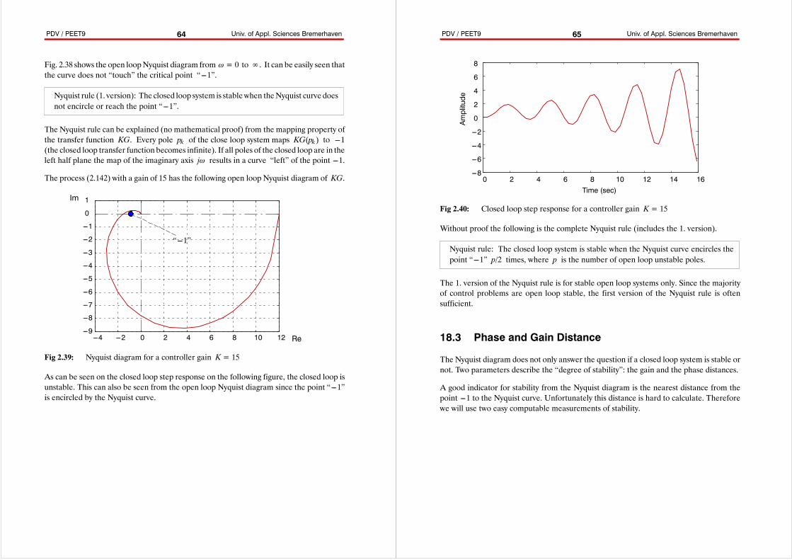
PDV / PEET9 Univ. of Appl. Sciences Bremerhaven64
Fig. 2.38 shows the open loopNyquist diagram from ω = 0 to ∞. It can be easily seen thatthe curve does not “touch” the critical point “---1”.
Nyquist rule (1. version): The closed loop system is stablewhen theNyquist curve doesnot encircle or reach the point “---1”.
The Nyquist rule can be explained (no mathematical proof) from the mapping property ofthe transfer function KG. Every pole pk of the close loop system maps KG(pk) to ---1(the closed loop transfer function becomes infinite). If all poles of the closed loop are in theleft half plane the map of the imaginary axis jω results in a curve “left” of the point ---1.
The process (2.142) with a gain of 15 has the following open loop Nyquist diagram of KG.
---4 ---2 0 2 4 6 8 10 12---9
---8
---7
---6
---5
---4
---3
---2
---1
0
1
Re
Im
“---1”
Fig 2.39: Nyquist diagram for a controller gain K = 15
As can be seen on the closed loop step response on the following figure, the closed loop isunstable. This can also be seen from the open loop Nyquist diagram since the point “---1”is encircled by the Nyquist curve.
PDV / PEET9 Univ. of Appl. Sciences Bremerhaven65
Time (sec)
Amplitude
0 2 4 6 8 10 12 14 16---8
---6
---4
---2
0
2
4
6
8
Fig 2.40: Closed loop step response for a controller gain K = 15
Without proof the following is the complete Nyquist rule (includes the 1. version).
Nyquist rule: The closed loop system is stable when the Nyquist curve encircles thepoint “---1” p/2 times, where p is the number of open loop unstable poles.
The 1. version of the Nyquist rule is for stable open loop systems only. Since the majorityof control problems are open loop stable, the first version of the Nyquist rule is oftensufficient.
18.3 Phase and Gain Distance
The Nyquist diagram does not only answer the question if a closed loop system is stable ornot. Two parameters describe the “degree of stability”: the gain and the phase distances.
A good indicator for stability from the Nyquist diagram is the nearest distance from thepoint ---1 to the Nyquist curve. Unfortunately this distance is hard to calculate. Thereforewe will use two easy computable measurements of stability.
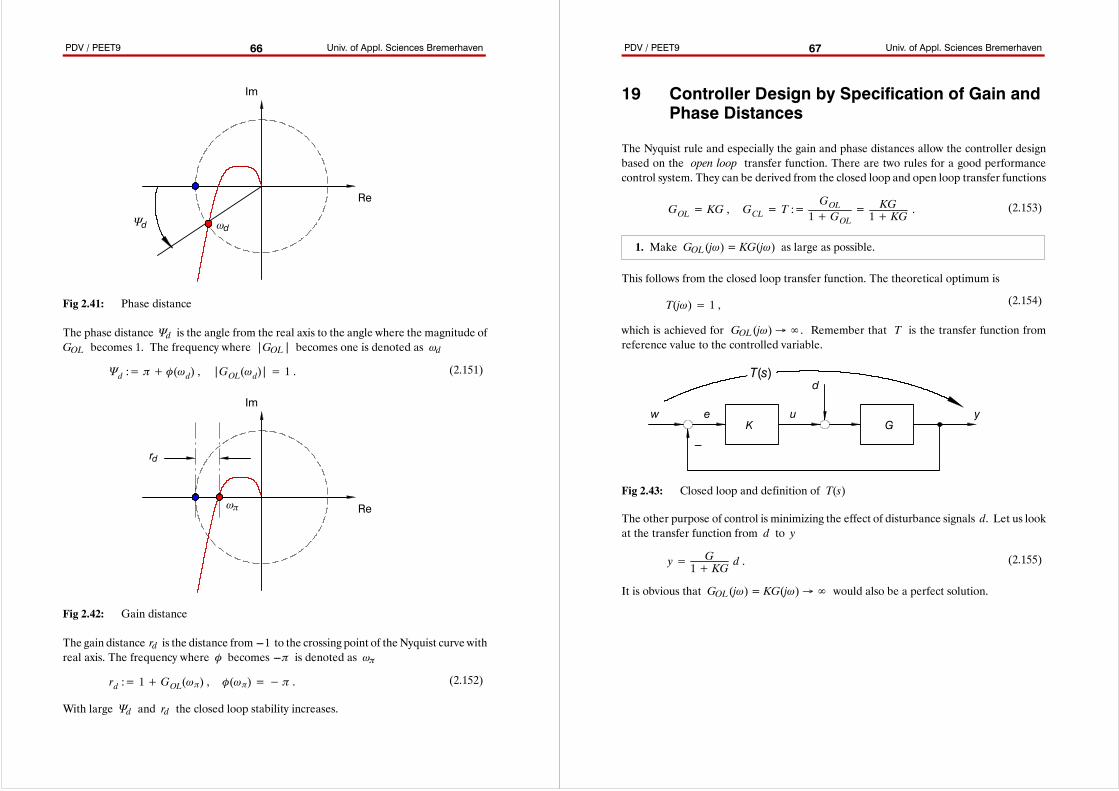
PDV / PEET9 Univ. of Appl. Sciences Bremerhaven66
Re
Im
Ψd ωd
Fig 2.41: Phase distance
The phase distance Ψd is the angle from the real axis to the angle where the magnitude ofGOL becomes 1. The frequency where |GOL| becomes one is denoted as ωd
Ψd := π+ Ô(ωd) , |GOL(ωd)|= 1 . (2.151)
Re
Im
ωπ
rd
Fig 2.42: Gain distance
The gain distance rd is the distance from ---1 to the crossing point of theNyquist curve withreal axis. The frequency where Ô becomes ---π is denoted as ωπ
rd := 1+GOL(ωπ) , Ô(ωπ)=− π . (2.152)
With large Ψd and rd the closed loop stability increases.
PDV / PEET9 Univ. of Appl. Sciences Bremerhaven67
19 Controller Design by Specification of Gain andPhase Distances
The Nyquist rule and especially the gain and phase distances allow the controller designbased on the open loop transfer function. There are two rules for a good performancecontrol system. They can be derived from the closed loop and open loop transfer functions
GOL= KG , GCL= T :=GOL1+GOL
= KG1+ KG .
(2.153)
1. Make GOL(jω) = KG(jω) as large as possible.
This follows from the closed loop transfer function. The theoretical optimum is
T(jω)= 1 , (2.154)
which is achieved for GOL(jω)→∞. Remember that T is the transfer function fromreference value to the controlled variable.
e u
d
yK G
w
---
T(s)
Fig 2.43: Closed loop and definition of T(s)
The other purpose of control is minimizing the effect of disturbance signals d. Let us lookat the transfer function from d to y
y= G1+ KG d .
(2.155)
It is obvious that GOL(jω) = KG(jω)→∞ would also be a perfect solution.
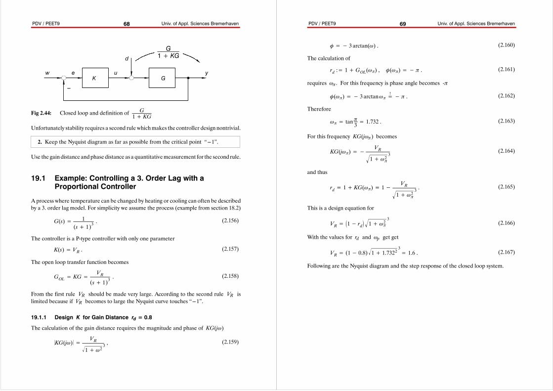
PDV / PEET9 Univ. of Appl. Sciences Bremerhaven68
e u
d
yK G
w
---
G1+ KG
Fig 2.44: Closed loop and definition of G1+ KG
Unfortunately stability requires a second rule whichmakes the controller designnontrivial.
2. Keep the Nyquist diagram as far as possible from the critical point “---1”.
Use the gain distance andphasedistance asa quantitativemeasurement for the secondrule.
19.1 Example: Controlling a 3. Order Lag with aProportional Controller
Aprocess where temperature can be changed by heating or cooling can often be describedby a 3. order lag model. For simplicity we assume the process (example from section 18.2)
G(s)= 1(s+ 1)3
. (2.156)
The controller is a P-type controller with only one parameter
K(s)= VR . (2.157)
The open loop transfer function becomes
GOL= KG=VR
(s+ 1)3. (2.158)
From the first rule VR should be made very large. According to the second rule VR islimited because if VR becomes to large the Nyquist curve touches “---1”.
19.1.1 Design K for Gain Distance rd = 0.8
The calculation of the gain distance requires the magnitude and phase of KG(jω)
KG(jω) =VR
1+ ω2 3 , (2.159)
PDV / PEET9 Univ. of Appl. Sciences Bremerhaven69
Ô=− 3 arctan(ω) . (2.160)
The calculation of
rd := 1+GOL(ωπ) , Ô(ωπ)=− π . (2.161)
requires ωπ. For this frequency is phase angle becomes -π
Ô(ωπ)=− 3 arctanωπ=! − π . (2.162)
Therefore
ωπ= tanπ3 = 1.732 .(2.163)
For this frequency KG(jωπ) becomes
KG(jωπ)=−VR
1+ ω2π 3(2.164)
and thus
rd= 1+ KG(ωπ)= 1−VR
1+ ω2π 3 . (2.165)
This is a design equation for
VR= 1− rd 1+ ω2π 3(2.166)
With the values for rd and ωp get get
VR= (1− 0.8) 1+ 1.7322 3= 1.6 . (2.167)
Following are the Nyquist diagram and the step response of the closed loop system.
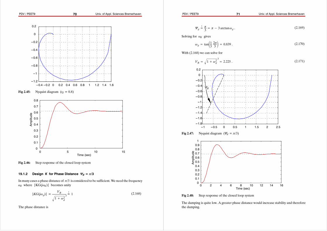
PDV / PEET9 Univ. of Appl. Sciences Bremerhaven70
---0.4 ---0.2 0 0.2 0.4 0.6 0.8 1 1.2 1.4 1.6---1.2
---1
---0.8
---0.6
---0.4
---0.2
0
0.2
Fig 2.45: Nyquist diagram (rd = 0.8)
Time (sec)
Amplitude
0 5 10 150
0.1
0.2
0.3
0.4
0.5
0.6
0.7
0.8
Fig 2.46: Step response of the closed loop system
19.1.2 Design K for Phase Distance Ψd = π/3
Inmany cases a phase distance of π/3 is considered to be sufficient.We need the frequencyωd where |KG(jωd)| becomes unity
|KG(jωd)|=VR
1+ ω2d
3=! 1 (2.168)
The phase distance is
PDV / PEET9 Univ. of Appl. Sciences Bremerhaven71
Ψd=! π3 = π− 3 arctanωd .
(2.169)
Solving for ωd gives
ωd= tan13 2π3 = 0.839 . (2.170)
With (2.168) we can solve for
VR= 1+ ω2d 3= 2.225 . (2.171)
---1 ---0.5 0 0.5 1 1.5 2 2.5---1.8
---1.6
---1.4
---1.2
---1
---0.8
---0.6
---0.4
---0.2
0
0.2
Ψd
Fig 2.47: Nyquist diagram (Ψd = π/3)
Time (sec)Amplitude
0 2 4 6 8 10 12 14 1600.10.20.30.40.50.60.70.80.91
Fig 2.48: Step response of the closed loop system
The damping is quite low. A greater phase distance would increase stability and thereforethe damping.
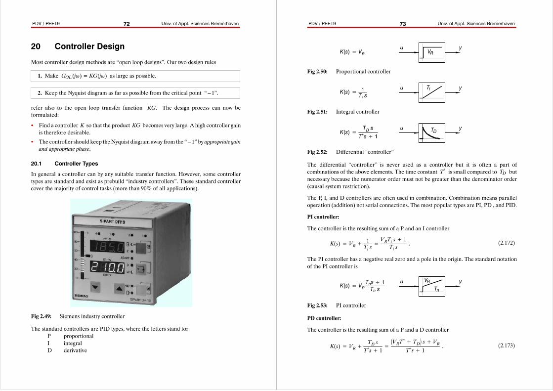
PDV / PEET9 Univ. of Appl. Sciences Bremerhaven72
20 Controller Design
Most controller design methods are “open loop designs”. Our two design rules
1. Make GOL(jω) = KG(jω) as large as possible.
2. Keep the Nyquist diagram as far as possible from the critical point “---1”.
refer also to the open loop transfer function KG. The design process can now beformulated:
S Find a controller K so that the product KG becomes very large. A high controller gainis therefore desirable.
S The controller should keep theNyquist diagram away from the “---1” by appropriate gainand appropriate phase.
20.1 Controller Types
In general a controller can by any suitable transfer function. However, some controllertypes are standard and exist as prebuild “industry controllers”. These standard controllercover the majority of control tasks (more than 90% of all applications).
Fig 2.49: Siemens industry controller
The standard controllers are PID types, where the letters stand forP proportionalI integralD derivative
PDV / PEET9 Univ. of Appl. Sciences Bremerhaven73
u yVRK(s)= VR
Fig 2.50: Proportional controller
u yTiK(s)= 1Ti s
Fig 2.51: Integral controller
u yTDK(s)=TD sT*s+ 1
Fig 2.52: Differential “controller”
The differential “controller” is never used as a controller but it is often a part ofcombinations of the above elements. The time constant T* is small compared to TD butnecessary because the numerator order must not be greater than the denominator order(causal system restriction).
The P, I, and D controllers are often used in combination. Combination means paralleloperation (addition) not serial connections. The most popular types are PI, PD , and PID.
PI controller:
The controller is the resulting sum of a P and an I controller
K(s)= VR+1Ti s=VRTi s+ 1Ti s
. (2.172)
The PI controller has a negative real zero and a pole in the origin. The standard notationof the PI controller is
u yTn
K(s)= VRTns+ 1Tn s
VR
Fig 2.53: PI controller
PD controller:
The controller is the resulting sum of a P and a D controller
K(s)= VR+TD sT*s+ 1
=VRT*+ TD s+ VR
T*s+ 1. (2.173)
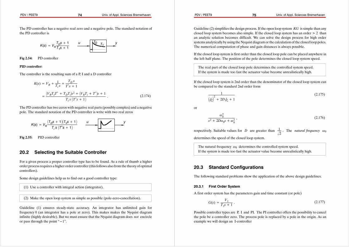
PDV / PEET9 Univ. of Appl. Sciences Bremerhaven74
The PD controller has a negative real zero and a negative pole. The standard notation ofthe PD controller is
u yT1K(s)= VRTDs+ 1T1s+ 1
TD
Fig 2.54: PD controller
PID controller:
The controller is the resulting sum of a P, I and a D controller
=VRTIT*+ TDTis2+ VRTi+ T*s+ 1
Ti s T*s+ 1. (2.174)
K(s)= VR+1Ti s+TD sT*s+ 1
The PD controller has two zeros with negative real parts (possibly complex) and a negativepole. The standard notation of the PD controller is write with two real zeros
u yK(s)= VR
TDs+ 1TVs+ 1Ti s T*s+ 1
Fig 2.55: PID controller
20.2 Selecting the Suitable Controller
For a given process a proper controller type has to be found. As a rule of thumb a higherorder process requires a higher order controller (this follows also from the theory ofoptimalcontrollers).
Some design guidelines help us to find out a good controller type:
(1) Use a controller with integral action (integrator).
(2) Make the open loop system as simple as possible (pole-zero-cancellation).
Guideline (1) ensures steady-state accuracy. An integrator has unlimited gain forfrequency 0 (an integrator has a pole at zero). This makes makes the Nyquist diagraminfinite (highly desirable). But we must ensure that the Nyquist diagram does not encircleor pass through the point “---1”.
PDV / PEET9 Univ. of Appl. Sciences Bremerhaven75
Guideline (2) simplifies the design process. If the open loop system KG is simple than anyclosed loop system becomes also simple. If the closed loop system has an order > 2 thanan analytic solution becomes difficult. We can solve the design process for high ordersystems analytically by using theNyquist diagramor the calculationof the closed looppoles.The numerical computation of phase and gain distances is always possible.
If the closed loop system is first order than the closed loop pole can be placed anywhere inthe left half plane. The position of the pole determines the closed loop system speed.
The real part of the closed loop pole determines the controlled system speed.If the system is made too fast the actuator value become unrealistically high.
If the closed loop system is 2nd order than the denominator of the closed loop system canbe compared to the standard 2nd order form
1
sω02+ 2D s
ω0+ 1(2.175)
or
ω20s2+ 2Dω0s+ ω20
, (2.176)
respectively. Suitable values for D are greater than 12. The natural frequency ω0
determines the speed of the closed loop system.
The natural frequency ω0 determines the controlled system speed.If the system is made too fast the actuator value become unrealistically high.
20.3 Standard Configurations
The following standard problems show the application of the above design guidelines.
20.3.1 First Order System
A first order system has the parameters gain and time constant (or pole)
G(s)=V1
T1s+ 1. (2.177)
Possible controller types are P, I and PI. The PI controller offers the possibility to cancelthe pole be a controller zero. The process pole is replaced by a pole in the origin. As anexample we will design an I-controller
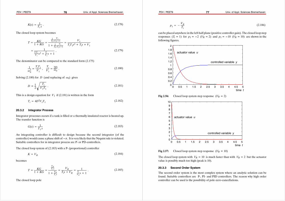
PDV / PEET9 Univ. of Appl. Sciences Bremerhaven76
K(s)= 1Ti s. (2.178)
The closed loop system becomes
= 1TiT1V1s2+ Ti
V1s+ 1
. (2.179)
T= KG1+ KG=
1Tis
V1T1s+1
1+ 1Tis
V1T1s+1
=V1
TiT1s2+ Tis+ V1
The denominator can be compared to the standard form (2.175)
1ω20=TiT1V1,TiV1= 2Dω0
. (2.180)
Solving (2.180) for D (and replacing of ω0) gives
D= 12TiV1T1 . (2.181)
This is a design equation for V1 if (2.181) is written in the form
Ti= 4D2V1T1 (2.182)
20.3.2 Integrator Process
Integrator processes occurs if a tank is filled or a thermally insulated reactor is heated up.The transfer function is
G(s)= 1T1 s
(2.183)
An integrating controller is difficult to design because the second integrator (of thecontroller) would cause a phase shift of ---π. It is very likely that theNyquist rule is violated.Suitable controllers for in integrator process are P- or PD-controllers.
The closed loop system of (2.183) with a P- (proportional) controller
K= VR (2.184)
becomes
T= KG1+ KG=
VRTi s
1+ VRTi s
=VR
Tis+ VR= 1TiVRs+ 1
. (2.185)
The closed loop pole
PDV / PEET9 Univ. of Appl. Sciences Bremerhaven77
p1=−VRTi
(2.186)
canbe placed anywhere in the left half plane (positive controller gain). The closed loop stepresponses (Ti = 1) for p1 = ---2 (VR = 2) and p1 = ---10 (VR = 10) are shown in thefollowing figures.
0 0.5 1 1.5 2 2.5 3 3.5 4 4.5 500.20.40.60.811.21.41.61.82
time t
actuator value u
controlled variable y
Fig 2.56: Closed loop system step response (VR = 2)
0 0.5 1 1.5 2 2.5 3 3.5 4 4.5 5012345678910
time t
actuator value u
controlled variable y
Fig 2.57: Closed loop system step response (VR = 10)
The closed loop system with VR = 10 is much faster than with VR = 2 but the actuatorvalue is possibly much too high (peak is 10).
20.3.3 Second Order System
The second order system is the most complex system where an analytic solution can befound. Suitable controllers are P-, PI- and PID controllers. The reason why high ordercontroller can be used is the possibility of pole-zero-cancellations.
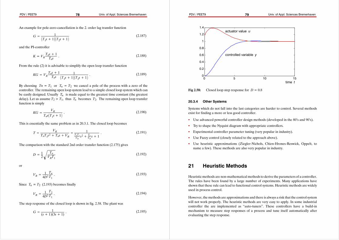
PDV / PEET9 Univ. of Appl. Sciences Bremerhaven78
An example for pole-zero-cancellation is the 2. order lag transfer function
G= 1T1s+ 1T2s+ 1
(2.187)
and the PI-controller
K= VRTns+ 1Tns
. (2.188)
From the rule (2) it is advisable to simplify the open loop transfer function
KG= VRTns+ 1Tns
1T1s+ 1T2s+ 1
. (2.189)
By choosing Tn = T1 or Tn = T2 we cancel a pole of the process with a zero of thecontroller. The remaining open loop system lead to a simple closed loop system which canbe easily designed. Usually Tn is made equal to the greatest time constant (the greatestdelay). Let us assume T2 > T1, thus Tn becomes T2. The remaining open loop transferfunction is simply
KG=VR
TnsT1s+ 1. (2.190)
This is essentially the same problem as in 20.3.1. The closed loop becomes
T=VR
TnT1s2+ Tns+ VR= 1TnT1VRs2+ Tn
VRs+ 1
. (2.191)
The comparison with the standard 2nd order transfer function (2.175) gives
D= 12TnVRT1 (2.192)
or
VR=14D2TnT1. (2.193)
Since Tn = T2 (2.193) becomes finally
VR=14D2T2T1. (2.194)
The step response of the closed loop is shown in fig. 2.58. The plant was
G= 1(s+ 1)(3s+ 1)
. (2.195)
PDV / PEET9 Univ. of Appl. Sciences Bremerhaven79
0 5 10 150
0.2
0.4
0.6
0.8
1
1.2
1.4
time t
actuator value u
controlled variable y
Fig 2.58: Closed loop step response for D = 0.8
20.3.4 Other Systems
Systems which do not fall into the last categories are harder to control. Several methodsexist for finding a more or less good controller.
S Use advanced powerful controller design methods (developed in the 80’s and 90’s).
S Try to shape the Nyquist diagram with appropriate controllers.
S Experimental controller parameter tuning (very popular in industry).
S Use Fuzzy control (closely related to the approach above).
S Use heuristic approximations (Ziegler-Nichols, Chien-Hrones-Reswick, Oppelt, toname a few). These methods are also very popular in industry.
21 Heuristic Methods
Heuristic methods are non-mathematical methods to derive the parameters of a controller.The rules have been found by a large number of experiments. Many applications haveshown that these rule can lead to functional control systems. Heuristic methods are widelyused in process control.
However, themethods are approximations and there is always a risk that the control systemwill not work properly. The heuristic methods are very easy to apply. In some industrialcontroller the are implemented as “auto-tuners”. These controllers have a build-inmechanism to measure step responses of a process and tune itself automatically afterevaluating the step response.
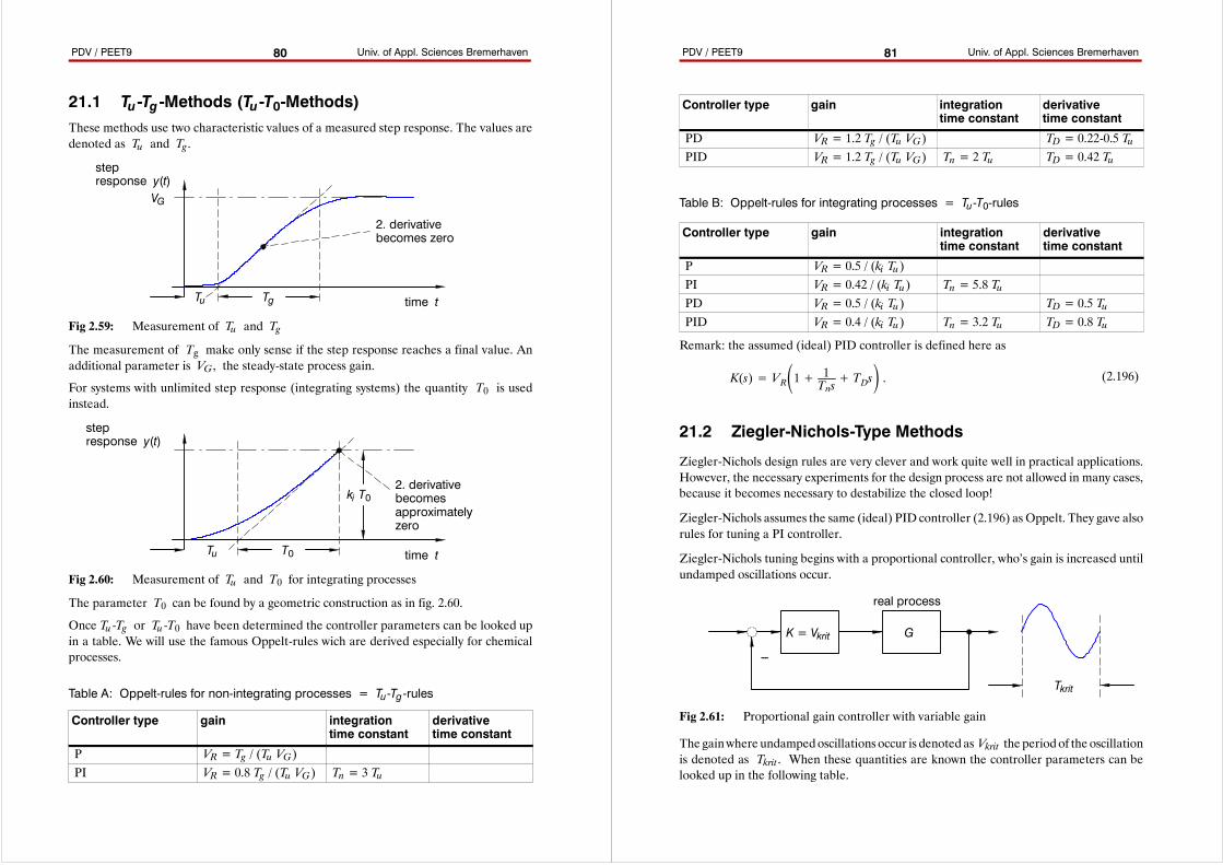
PDV / PEET9 Univ. of Appl. Sciences Bremerhaven80
21.1 Tu -Tg -Methods (Tu -T0-Methods)These methods use two characteristic values of a measured step response. The values aredenoted as Tu and Tg .
Tu Tg time t
stepresponse y(t)
2. derivativebecomes zero
VG
Fig 2.59: Measurement of Tu and Tg
The measurement of Tg make only sense if the step response reaches a final value. Anadditional parameter is VG , the steady-state process gain.
For systems with unlimited step response (integrating systems) the quantity T0 is usedinstead.
Tu T0 time t
stepresponse y(t)
2. derivativebecomesapproximatelyzero
ki T0
Fig 2.60: Measurement of Tu and T0 for integrating processes
The parameter T0 can be found by a geometric construction as in fig. 2.60.
Once Tu -Tg or Tu -T0 have been determined the controller parameters can be looked upin a table. We will use the famous Oppelt-rules wich are derived especially for chemicalprocesses.
Table A: Oppelt-rules for non-integrating processes = Tu-Tg-rules
Controller type gain integrationtime constant
derivativetime constant
P VR = Tg / (Tu VG)PI VR = 0.8 Tg / (Tu VG) Tn = 3 Tu
PDV / PEET9 Univ. of Appl. Sciences Bremerhaven81
Controller type derivativetime constant
integrationtime constant
gain
PD VR = 1.2 Tg / (Tu VG) TD = 0.22-0.5 TuPID VR = 1.2 Tg / (Tu VG) Tn = 2 Tu TD = 0.42 Tu
Table B: Oppelt-rules for integrating processes = Tu-T0-rules
Controller type gain integrationtime constant
derivativetime constant
P VR = 0.5 / (ki Tu)PI VR = 0.42 / (ki Tu) Tn = 5.8 TuPD VR = 0.5 / (ki Tu) TD = 0.5 TuPID VR = 0.4 / (ki Tu) Tn = 3.2 Tu TD = 0.8 Tu
Remark: the assumed (ideal) PID controller is defined here as
K(s)= VR1+ 1Tns+ TDs . (2.196)
21.2 Ziegler-Nichols-Type Methods
Ziegler-Nichols design rules are very clever and work quite well in practical applications.However, the necessary experiments for the design process are not allowed in many cases,because it becomes necessary to destabilize the closed loop!
Ziegler-Nichols assumes the same (ideal) PID controller (2.196) as Oppelt. They gave alsorules for tuning a PI controller.
Ziegler-Nichols tuning begins with a proportional controller, who’s gain is increased untilundamped oscillations occur.
K = Vkrit G
real process
---
Tkrit
Fig 2.61: Proportional gain controller with variable gain
The gainwhere undampedoscillations occur is denoted as Vkrit the periodof the oscillationis denoted as Tkrit . When these quantities are known the controller parameters can belooked up in the following table.
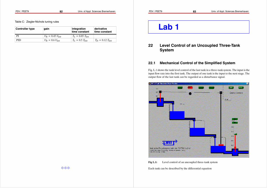
PDV / PEET9 Univ. of Appl. Sciences Bremerhaven82
Table C: Ziegler-Nichols tuning rules
Controller type gain integrationtime constant
derivativetime constant
PI VR = 0.45 Vkrit Tn = 0.85 TkritPID VR = 0.6 Vkrit Tn = 0.5 Tkrit TD = 0.12 Tkrit
:::
PDV / PEET9 Univ. of Appl. Sciences Bremerhaven83
Lab 1
22 Level Control of an Uncoupled Three-TankSystem
22.1 Mechanical Control of the Simplified System
Fig. L.1 shows the tank level control of the last tank in a three-tank system. The input is theinput flow rate into the first tank. The output of one tank is the input to the next stage. Theoutput flow of the last tank can be regarded as a disturbance signal.
Fig L.1: Level control of an uncoupled three-tank system
Each tank can be described by the differential equation
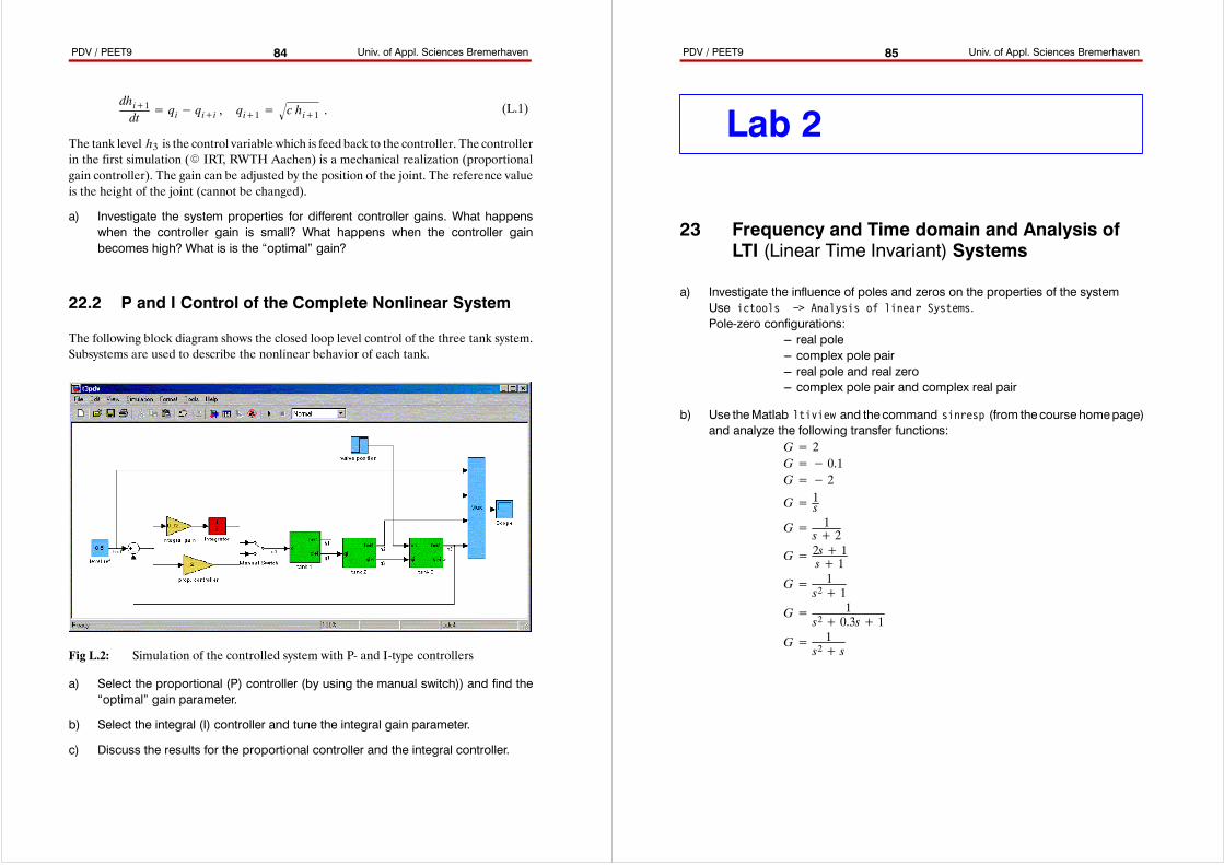
PDV / PEET9 Univ. of Appl. Sciences Bremerhaven84
dhi+1dt= qi− qi+i , qi+1= c hi+1 . (L.1)
The tank level h3 is the control variable which is feed back to the controller. The controllerin the first simulation (E IRT, RWTH Aachen) is a mechanical realization (proportionalgain controller). The gain can be adjusted by the position of the joint. The reference valueis the height of the joint (cannot be changed).
a) Investigate the system properties for different controller gains. What happenswhen the controller gain is small? What happens when the controller gainbecomes high? What is is the “optimal” gain?
22.2 P and I Control of the Complete Nonlinear System
The following block diagram shows the closed loop level control of the three tank system.Subsystems are used to describe the nonlinear behavior of each tank.
Fig L.2: Simulation of the controlled system with P- and I-type controllers
a) Select the proportional (P) controller (by using the manual switch)) and find the“optimal” gain parameter.
b) Select the integral (I) controller and tune the integral gain parameter.
c) Discuss the results for the proportional controller and the integral controller.
PDV / PEET9 Univ. of Appl. Sciences Bremerhaven85
Lab 2
23 Frequency and Time domain and Analysis ofLTI (Linear Time Invariant) Systems
a) Investigate the influence of poles and zeros on the properties of the systemUse ictools -> Analysis of linear Systems.Pole-zero configurations:
--- real pole--- complex pole pair--- real pole and real zero--- complex pole pair and complex real pair
b) Use theMatlab ltiview and thecommand sinresp (from thecourse homepage)and analyze the following transfer functions:
G= 2G=− 0.1G=− 2
G= 1sG= 1
s+ 2G= 2s+ 1
s+ 1G= 1
s2+ 1G= 1
s2+ 0.3s+ 1G= 1
s2+ s
PDV / PEET9 Univ. of Appl. Sciences Bremerhaven86
Lab 3
24 Impact of Zeros and Poles on ProcessProperties
Poles and zeros characterize the process. This is important for closed loop systems wherethepolesdetermine systemstability. The zeros affect the transfer characteristic with respectto the system input since they are associated by the transfer function numerator.
Investigate the influence of poles and zeros on the frequency response.Use pzplane to enter the poles and zeros.Format to enter poles or zeros:
[ real1 imag1; real2 imag2; ...; realn imagn]If you enter a complex pole or zero, be sure to add the conjugate complex too!
Use ltiview to view the Nyquist diagram and the step response (the Bodediagram is drawn with pzplane).
Analyze the following transfer functions:
a) Integrator G(s)= 1s
b) First order lag G(s)= 1s+ 1 , G(s)=
15s+ 1
a) Second order lag G(s)= 1(s+ 1)(s+ 3)
a) Complex poles on the imaginary axis G(s)= 1s2+ 1
a) Complex poles and complex zeros on the imaginary axis G(s)= s2+ 1s2+ 4
a) Complex poles in the left half plane G(s)= 1s2+ 0.2s+ 1.01
a) PI controller G(s)= 3 2s+ 12s
PDV / PEET9 Univ. of Appl. Sciences Bremerhaven87
25 References
[1] Bateson, R.: Introduction to Control System Technology.Prentice Hall, 1999
[2] Denn, M.: Process Modelling.Wiley, 1986
[3] Doyle, F. et. al.: Process Control Modules.Prentice Hall, 2000
[4] Luyben, M. et. al.: Essentials of Process Control.McGraw-Hill, 1997
[5] Morari, M.: Robust Process Control.Prentice Hall, 1989
[6] Ogata, M.: Modern Control Engineering.Prentice Hall, 1997
[7] Seider, W. et. al.: Process Design Principles.Wiley, 1999