Embed Size (px)
Citation preview
Introductory Lecture II:
An Overview of Space Storms
Jan J. Sojka
Center for Atmospheric and Space Science
Utah State University
Logan, Utah
28 July 2010
Heliophysics Summer School Year IV 28 July - 4 August 2010
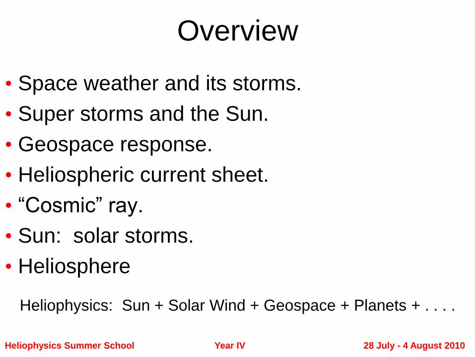
Overview
• Space weather and its storms.
• Super storms and the Sun.
• Geospace response.
• Heliospheric current sheet.
• “Cosmic” ray.
• Sun: solar storms.
• Heliosphere
Heliophysics: Sun + Solar Wind + Geospace + Planets + . . . .
Heliophysics Summer School Year IV 28 July - 4 August 2010
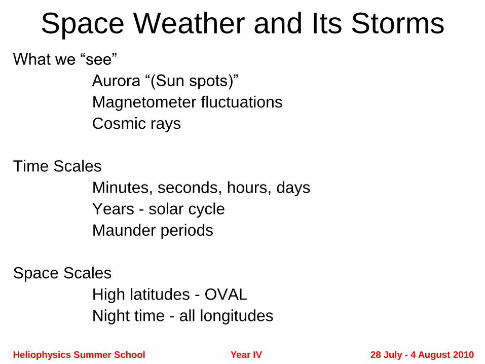
Space Weather and Its StormsWhat we “see”
Aurora “(Sun spots)”
Magnetometer fluctuations
Cosmic rays
Time Scales
Minutes, seconds, hours, days
Years - solar cycle
Maunder periods
Space Scales
High latitudes - OVAL
Night time - all longitudes
Heliophysics Summer School Year IV 28 July - 4 August 2010
Heliophysics Summer School Year IV 28 July - 4 August 2010
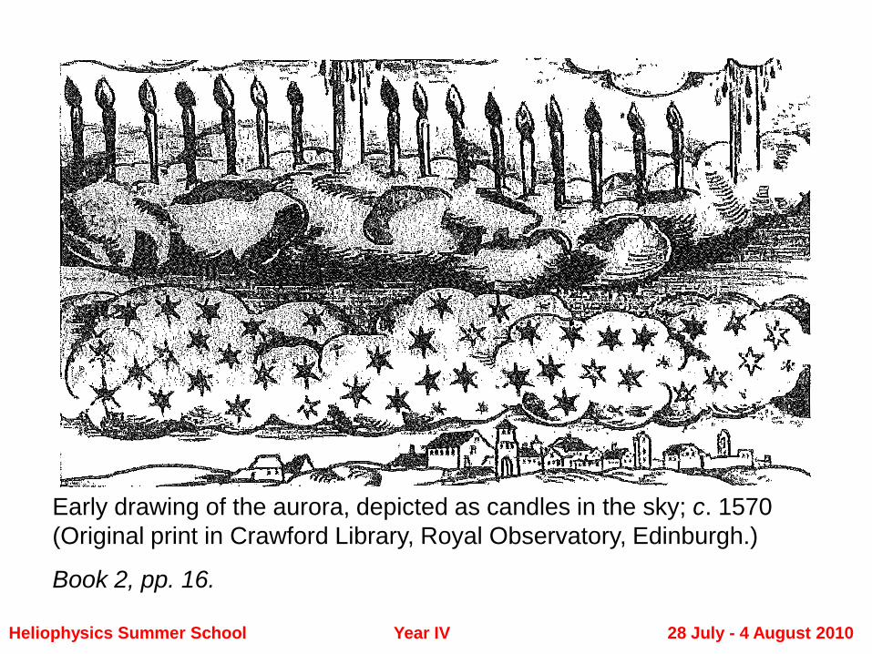
Early drawing of the aurora, depicted as candles in the sky; c. 1570
(Original print in Crawford Library, Royal Observatory, Edinburgh.)
Book 2, pp. 16.
Heliophysics Summer School Year IV 28 July - 4 August 2010
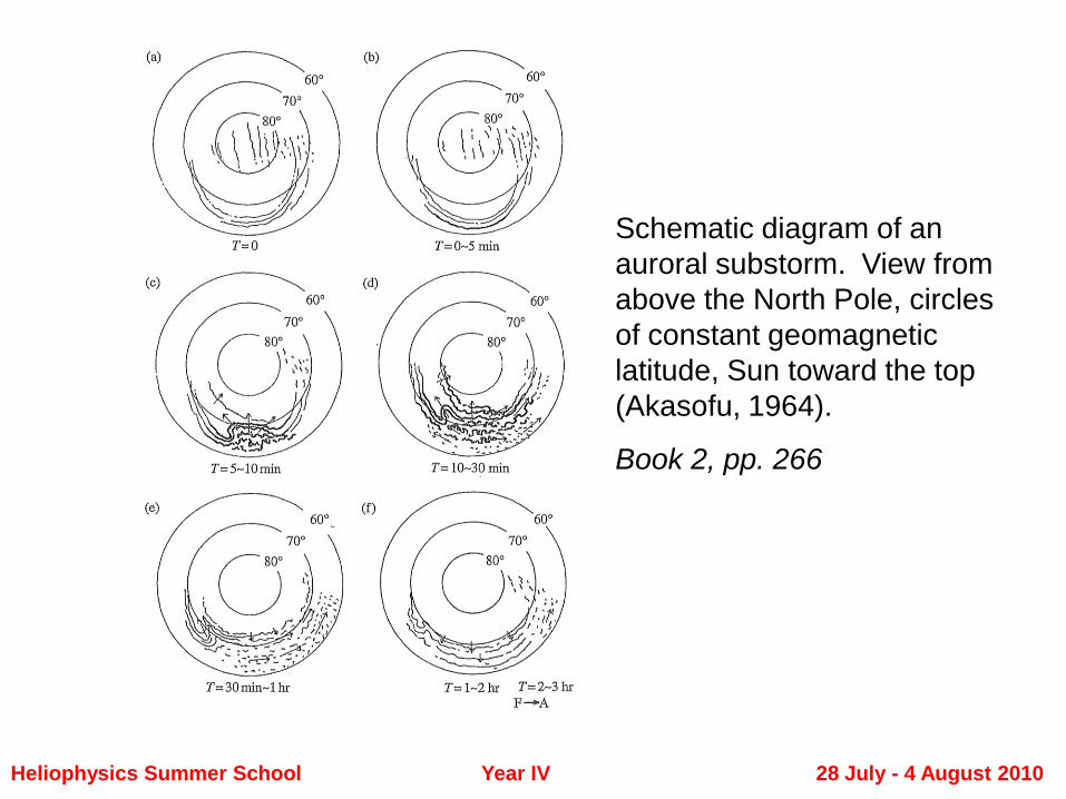
Schematic diagram of an
auroral substorm. View from
above the North Pole, circles
of constant geomagnetic
latitude, Sun toward the top
(Akasofu, 1964).
Book 2, pp. 266
Heliophysics Summer School Year IV 28 July - 4 August 2010
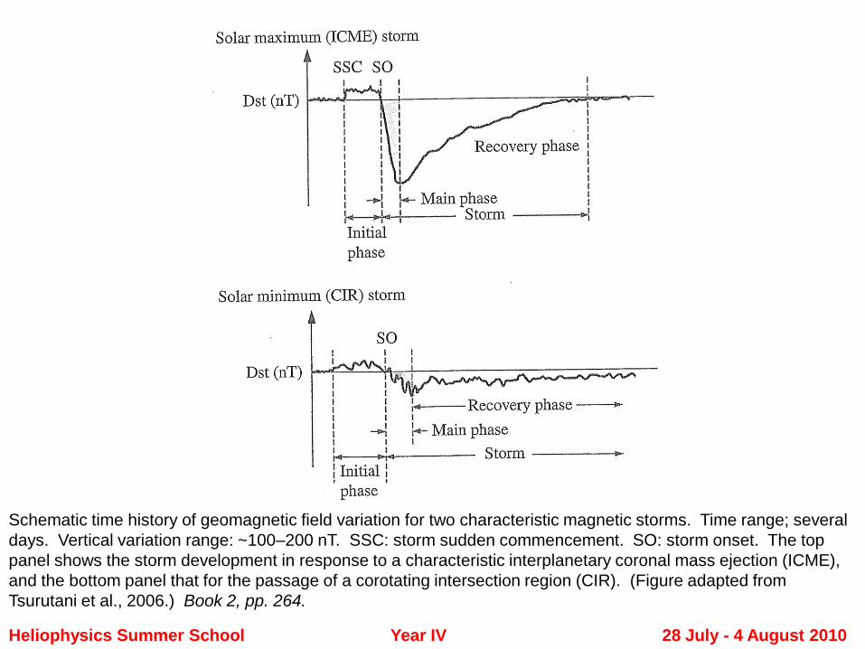
Schematic time history of geomagnetic field variation for two characteristic magnetic storms. Time range; several
days. Vertical variation range: ~100–200 nT. SSC: storm sudden commencement. SO: storm onset. The top
panel shows the storm development in response to a characteristic interplanetary coronal mass ejection (ICME),
and the bottom panel that for the passage of a corotating intersection region (CIR). (Figure adapted from
Tsurutani et al., 2006.) Book 2, pp. 264.
Heliophysics Summer School Year IV 28 July - 4 August 2010
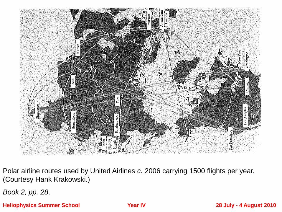
Polar airline routes used by United Airlines c. 2006 carrying 1500 flights per year.
(Courtesy Hank Krakowski.)
Book 2, pp. 28.

Back-of-the-Envelope Estimation
Given that United Airlines have 1500 polar crossing flights per year,
Estimate how many passengers take polar flights each year?
Note 1: you need to include an estimate for all airlines.
Note 2: Estimation means no calculators needed, no computers,…..
Heliophysics Summer School Year IV 28 July - 4 August 2010
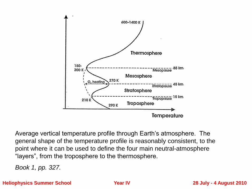
Average vertical temperature profile through Earth’s atmosphere. The
general shape of the temperature profile is reasonably consistent, to the
point where it can be used to define the four main neutral-atmosphere
“layers”, from the troposphere to the thermosphere.
Book 1, pp. 327.
Heliophysics Summer School Year IV 28 July - 4 August 2010
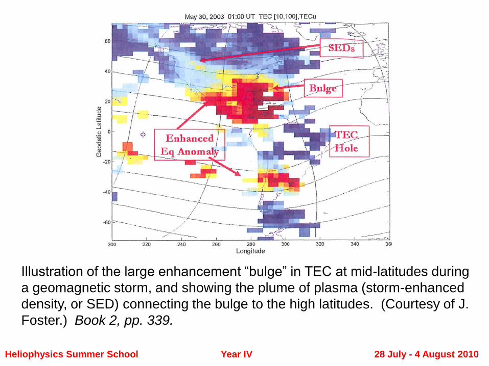
Illustration of the large enhancement “bulge” in TEC at mid-latitudes during
a geomagnetic storm, and showing the plume of plasma (storm-enhanced
density, or SED) connecting the bulge to the high latitudes. (Courtesy of J.
Foster.) Book 2, pp. 339.
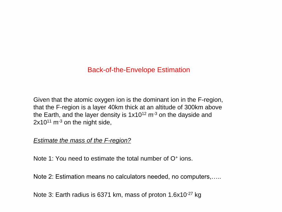
Back-of-the-Envelope Estimation
Given that the atomic oxygen ion is the dominant ion in the F-region,
that the F-region is a layer 40km thick at an altitude of 300km above
the Earth, and the layer density is 1x10¹² m-3 on the dayside and
2x10¹¹ m-3 on the night side,
Estimate the mass of the F-region?
Note 1: You need to estimate the total number of O+ ions.
Note 2: Estimation means no calculators needed, no computers,…..
Note 3: Earth radius is 6371 km, mass of proton 1.6x10⁻²⁷ kg
Heliophysics Summer School Year IV 28 July - 4 August 2010
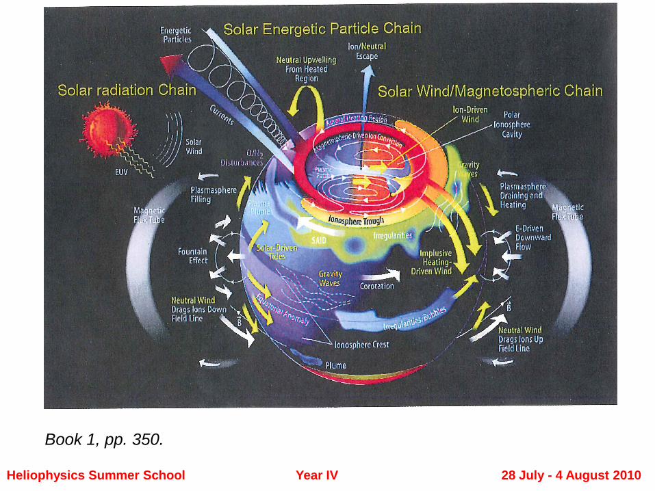
Book 1, pp. 350.
Super Storms and the Sun
• Carrington White Light Flare
1859, 1 September
• Coronal Mass Ejection (CME)
• High energy particles
• Time scales
Heliophysics Summer School Year IV 28 July - 4 August 2010
Heliophysics Summer School Year IV 28 July - 4 August 2010
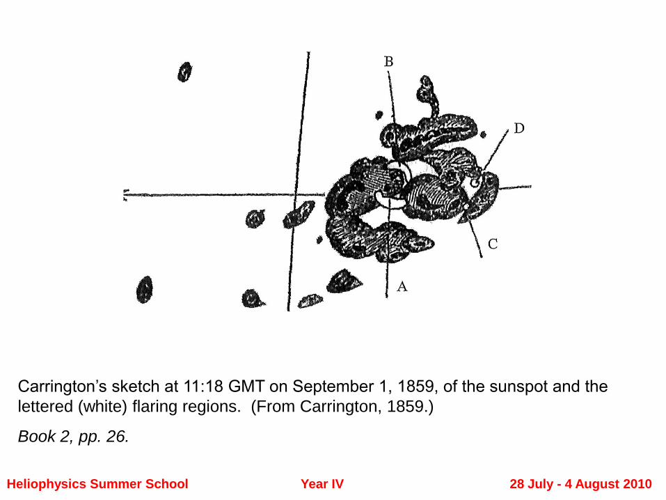
Carrington’s sketch at 11:18 GMT on September 1, 1859, of the sunspot and the
lettered (white) flaring regions. (From Carrington, 1859.)
Book 2, pp. 26.
Heliophysics Summer School Year IV 28 July - 4 August 2010
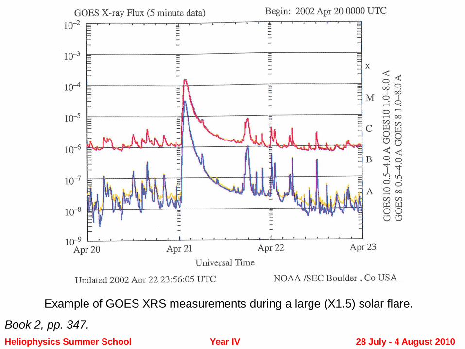
Example of GOES XRS measurements during a large (X1.5) solar flare.
Book 2, pp. 347.
Heliophysics Summer School Year IV 28 July - 4 August 2010
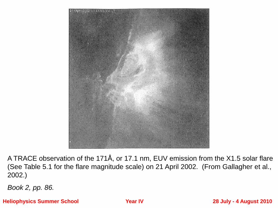
A TRACE observation of the 171Å, or 17.1 nm, EUV emission from the X1.5 solar flare
(See Table 5.1 for the flare magnitude scale) on 21 April 2002. (From Gallagher et al.,
2002.)
Book 2, pp. 86.
Back-of-the-Envelope Estimation
Given that light takes 8 minutes to travel from the Sun to the Earth,
Estimate how far the Earth is from the Sun ?
Note 1: Answer in km.
Note 2: Estimation means no calculators needed, no computers,…..
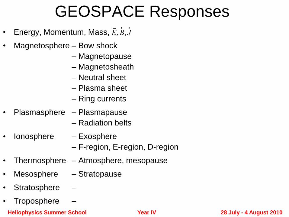
GEOSPACE Responses• Energy, Momentum, Mass,
• Magnetosphere – Bow shock
– Magnetopause
– Magnetosheath
– Neutral sheet
– Plasma sheet
– Ring currents
• Plasmasphere – Plasmapause
– Radiation belts
• Ionosphere – Exosphere
– F-region, E-region, D-region
• Thermosphere – Atmosphere, mesopause
• Mesosphere – Stratopause
• Stratosphere –
• Troposphere –
E,rB,
rJ
Heliophysics Summer School Year IV 28 July - 4 August 2010
Heliophysics Summer School Year IV 28 July - 4 August 2010
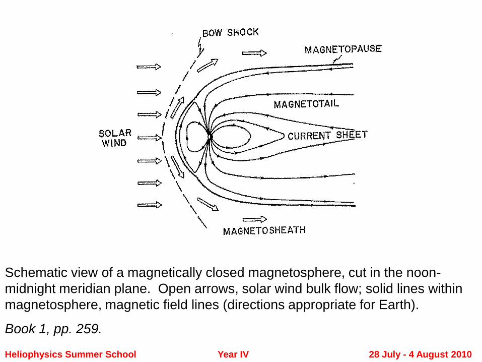
Schematic view of a magnetically closed magnetosphere, cut in the noon-
midnight meridian plane. Open arrows, solar wind bulk flow; solid lines within
magnetosphere, magnetic field lines (directions appropriate for Earth).
Book 1, pp. 259.
Heliophysics Summer School Year IV 28 July - 4 August 2010
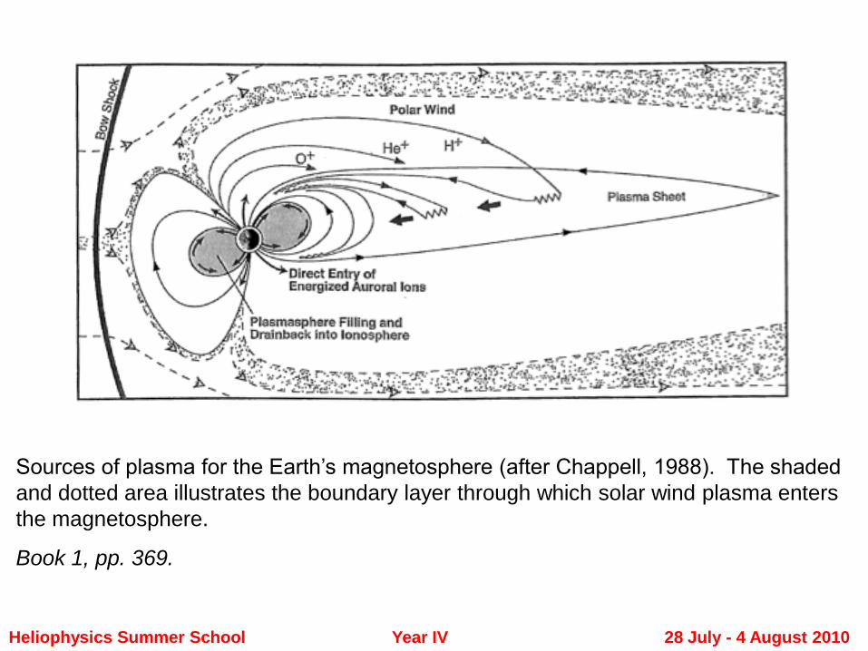
Sources of plasma for the Earth’s magnetosphere (after Chappell, 1988). The shaded
and dotted area illustrates the boundary layer through which solar wind plasma enters
the magnetosphere.
Book 1, pp. 369.
Back-of-the-Envelope Estimation
Given that the magnetosphere can be “viewed” as a cylinder that has
a diameter of 10 Re and a length of 60 Re, and that its total proton
content is approximately equal to the F-region O+ content,
Estimate the average proton density in the magnetosphere?
Note 1: Re is Earth radius.
Note 2: Estimation means no calculators needed, no computers,…..
Heliophysics Summer School Year IV 28 July - 4 August 2010
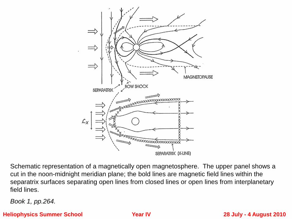
Schematic representation of a magnetically open magnetosphere. The upper panel shows a
cut in the noon-midnight meridian plane; the bold lines are magnetic field lines within the
separatrix surfaces separating open lines from closed lines or open lines from interplanetary
field lines.
Book 1, pp.264.
Heliophysics Summer School Year IV 28 July - 4 August 2010
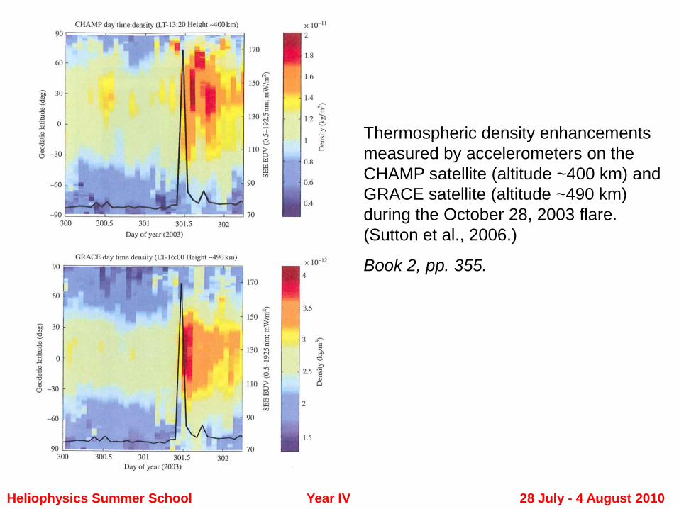
Thermospheric density enhancements
measured by accelerometers on the
CHAMP satellite (altitude ~400 km) and
GRACE satellite (altitude ~490 km)
during the October 28, 2003 flare.
(Sutton et al., 2006.)
Book 2, pp. 355.
Heliophysics Summer School Year IV 28 July - 4 August 2010
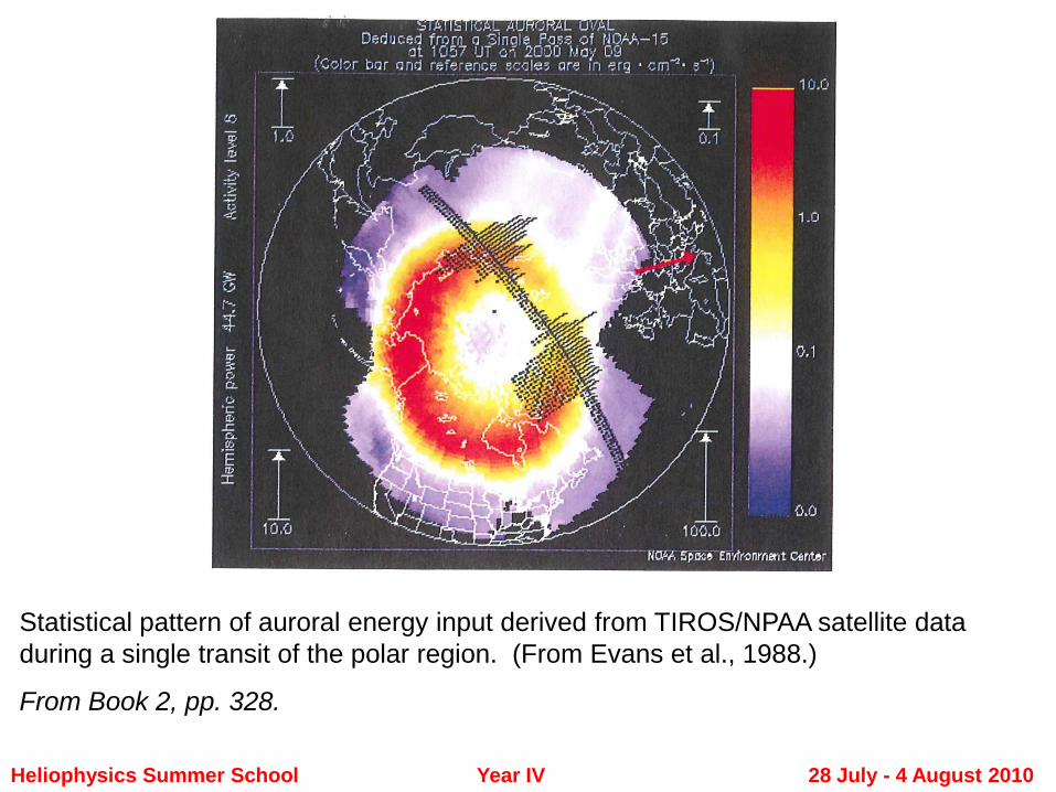
Statistical pattern of auroral energy input derived from TIROS/NPAA satellite data
during a single transit of the polar region. (From Evans et al., 1988.)
From Book 2, pp. 328.
Heliophysics Summer School Year IV 28 July - 4 August 2010
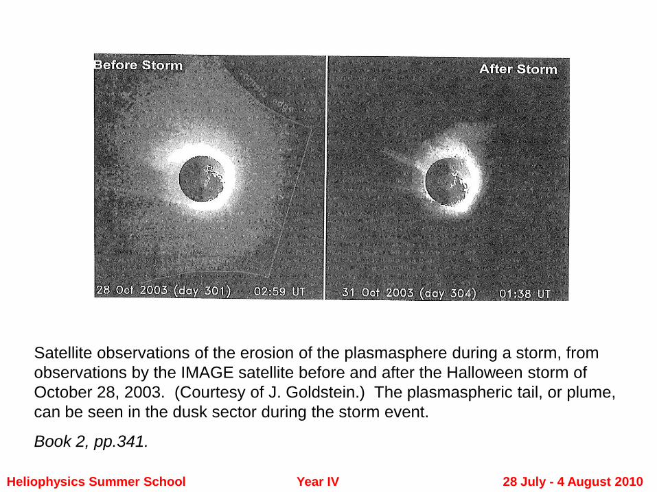
Satellite observations of the erosion of the plasmasphere during a storm, from
observations by the IMAGE satellite before and after the Halloween storm of
October 28, 2003. (Courtesy of J. Goldstein.) The plasmaspheric tail, or plume,
can be seen in the dusk sector during the storm event.
Book 2, pp.341.
Heliophysics Summer School Year IV 28 July - 4 August 2010
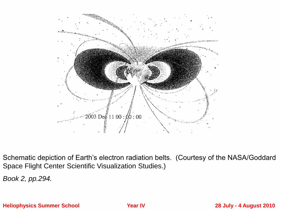
Schematic depiction of Earth’s electron radiation belts. (Courtesy of the NASA/Goddard
Space Flight Center Scientific Visualization Studies.)
Book 2, pp.294.
Heliospheric Current Sheet
• Solar wind
• Parker Spiral
• Solar rotation
• CME – Superstorm source
Heliophysics Summer School Year IV 28 July - 4 August 2010
Heliophysics Summer School Year IV 28 July - 4 August 2010
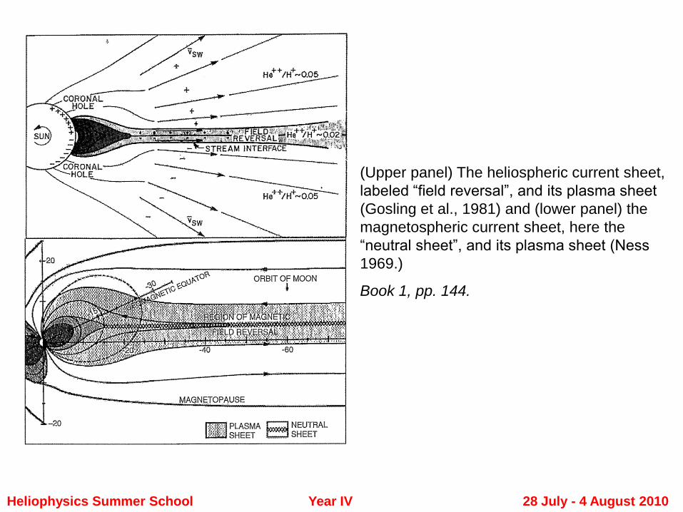
(Upper panel) The heliospheric current sheet,
labeled “field reversal”, and its plasma sheet
(Gosling et al., 1981) and (lower panel) the
magnetospheric current sheet, here the
“neutral sheet”, and its plasma sheet (Ness
1969.)
Book 1, pp. 144.
Heliophysics Summer School Year IV 28 July - 4 August 2010
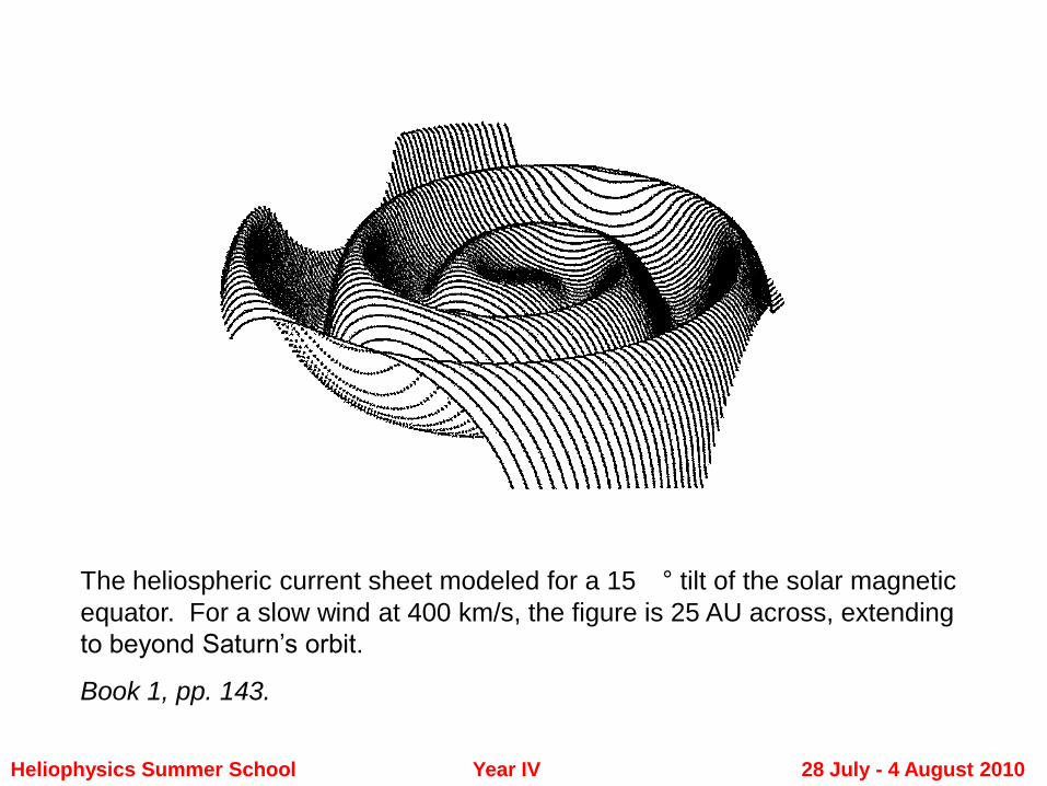
The heliospheric current sheet modeled for a 15�° tilt of the solar magnetic
equator. For a slow wind at 400 km/s, the figure is 25 AU across, extending
to beyond Saturn’s orbit.
Book 1, pp. 143.
Heliophysics Summer School Year IV 28 July - 4 August 2010
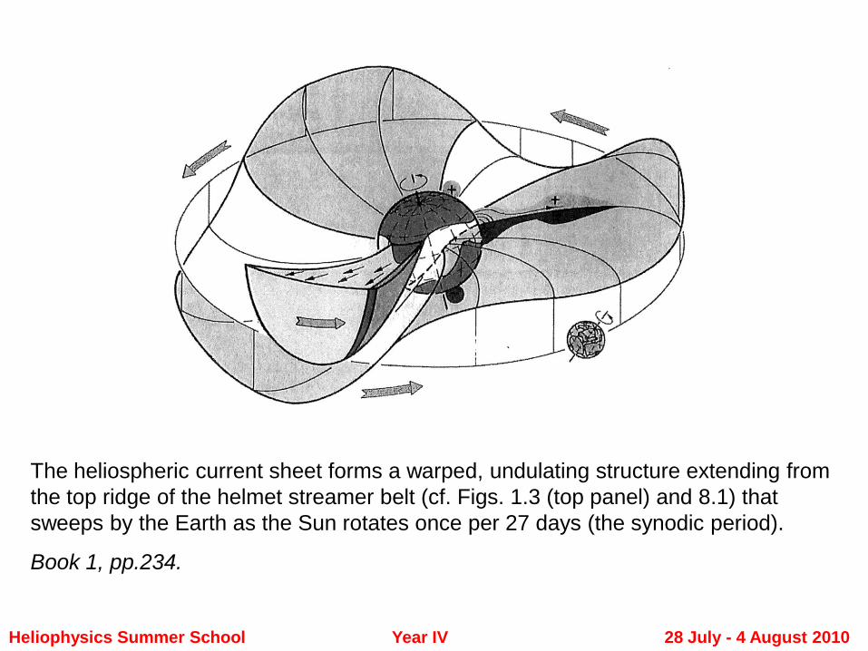
The heliospheric current sheet forms a warped, undulating structure extending from
the top ridge of the helmet streamer belt (cf. Figs. 1.3 (top panel) and 8.1) that
sweeps by the Earth as the Sun rotates once per 27 days (the synodic period).
Book 1, pp.234.
Heliophysics Summer School Year IV 28 July - 4 August 2010
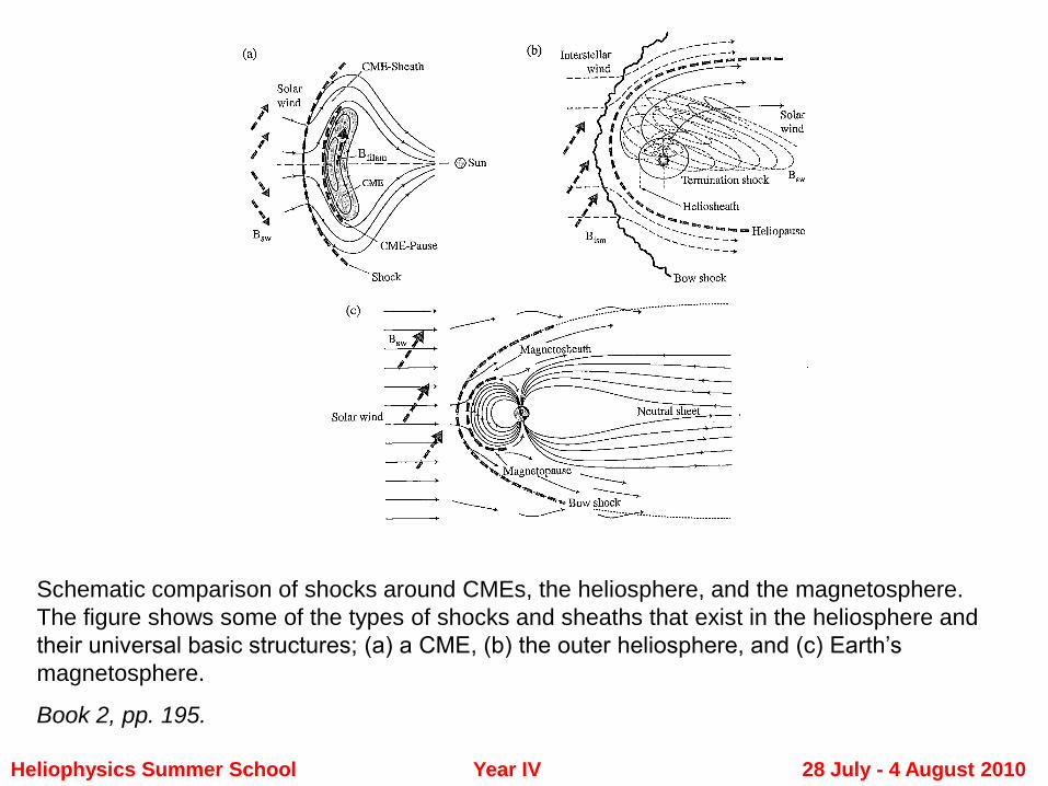
Schematic comparison of shocks around CMEs, the heliosphere, and the magnetosphere.
The figure shows some of the types of shocks and sheaths that exist in the heliosphere and
their universal basic structures; (a) a CME, (b) the outer heliosphere, and (c) Earth’s
magnetosphere.
Book 2, pp. 195.
Back-of-the-Envelope Estimation
Given a fast CME has an Earthward velocity of 1000km/s,
Estimate how long it takes to reach the Earth?
Note 1: Answer in units of hours
Note 2: Estimation means no calculators needed, no computers,…..
Heliophysics Summer School Year IV 28 July - 4 August 2010
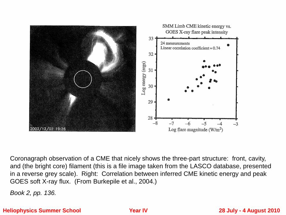
Coronagraph observation of a CME that nicely shows the three-part structure: front, cavity,
and (the bright core) filament (this is a file image taken from the LASCO database, presented
in a reverse grey scale). Right: Correlation between inferred CME kinetic energy and peak
GOES soft X-ray flux. (From Burkepile et al., 2004.)
Book 2, pp. 136.
“Cosmic” Rays Energization
• Acceleration of charged particles occurs in the Sun, in the solar wind, and in geospace.
• Van Alan Radiation Belts.
• Shocks in solar wind (CME, CIRs).
• Solar events generated solar energetic particles.
Heliophysics Summer School Year IV 28 July - 4 August 2010

Heliophysics Summer School Year IV 28 July - 4 August 2010
The explosive release of energy, mass, momentum, and magnetic field from (top
panel, SOHO-ESA and NASA) the solar corona.
Book 1, pp. 37.
Heliophysics Summer School Year IV 28 July - 4 August 2010
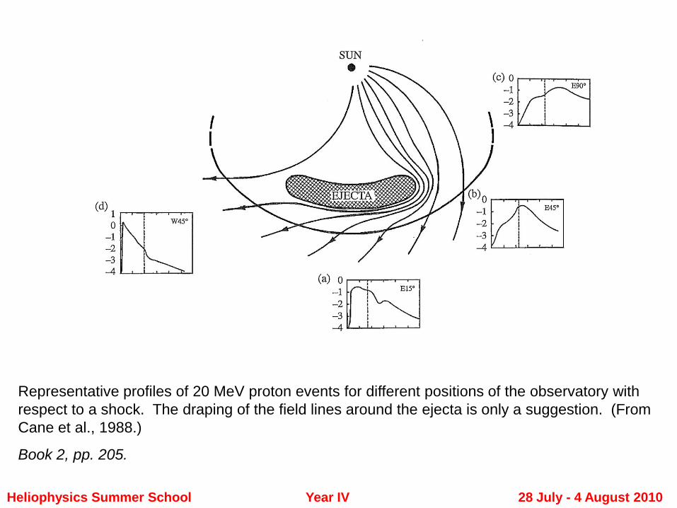
Representative profiles of 20 MeV proton events for different positions of the observatory with
respect to a shock. The draping of the field lines around the ejecta is only a suggestion. (From
Cane et al., 1988.)
Book 2, pp. 205.
Heliophysics Summer School Year IV 28 July - 4 August 2010
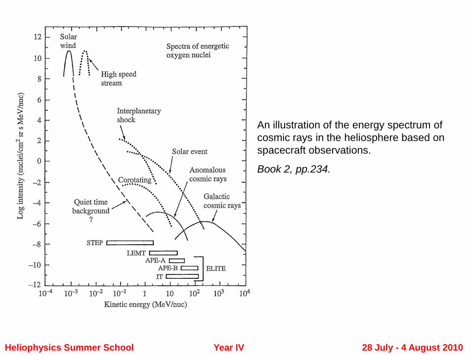
An illustration of the energy spectrum of
cosmic rays in the heliosphere based on
spacecraft observations.
Book 2, pp.234.
Back-of-the-Envelope Estimation
Given a solar produced energetic proton has an energy of 10MeV,
Estimate how long it takes to reach the Earth?
Note 1: Answer in units of hours
Note 2: Estimation means no calculators needed, no computers,…..
SUN: Solar Storms• Solar origin of space storms
• Layers – Convection zone– Photosphere– Chromosphere– Corona
• Features – Sun spots– Prominence– Flare loops– Coronal mass ejections– Fast streams– Slow solar wind– Reconnection sites
Heliophysics Summer School Year IV 28 July - 4 August 2010
Heliophysics Summer School Year IV 28 July - 4 August 2010
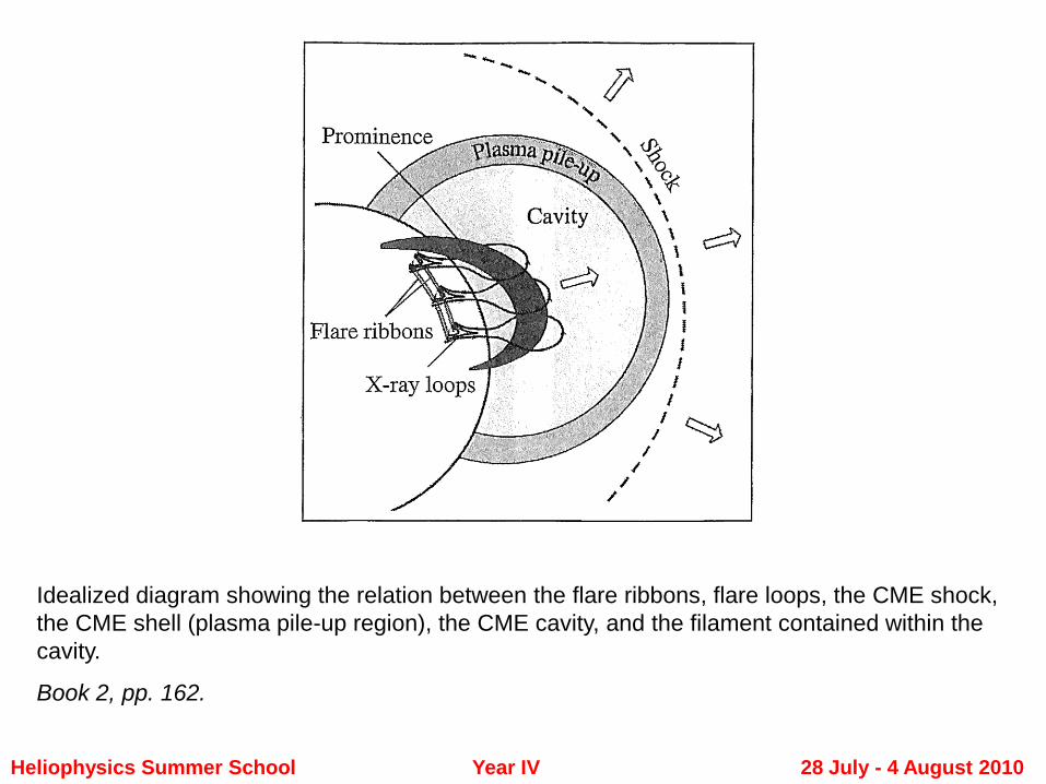
Idealized diagram showing the relation between the flare ribbons, flare loops, the CME shock,
the CME shell (plasma pile-up region), the CME cavity, and the filament contained within the
cavity.
Book 2, pp. 162.
Heliophysics Summer School Year IV 28 July - 4 August 2010
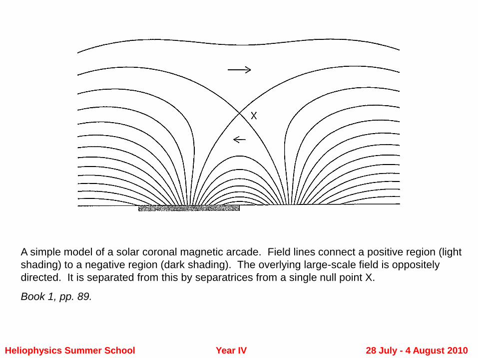
A simple model of a solar coronal magnetic arcade. Field lines connect a positive region (light
shading) to a negative region (dark shading). The overlying large-scale field is oppositely
directed. It is separated from this by separatrices from a single null point X.
Book 1, pp. 89.
Heliophysics Summer School Year IV 28 July - 4 August 2010
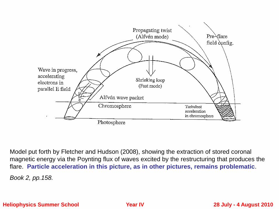
Model put forth by Fletcher and Hudson (2008), showing the extraction of stored coronal
magnetic energy via the Poynting flux of waves excited by the restructuring that produces the
flare. Particle acceleration in this picture, as in other pictures, remains problematic.
Book 2, pp.158.
Heliophysics Summer School Year IV 28 July - 4 August 2010
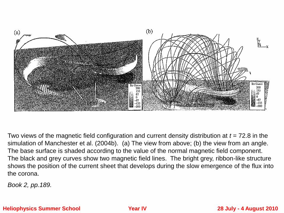
Two views of the magnetic field configuration and current density distribution at t = 72.8 in the
simulation of Manchester et al. (2004b). (a) The view from above; (b) the view from an angle.
The base surface is shaded according to the value of the normal magnetic field component.
The black and grey curves show two magnetic field lines. The bright grey, ribbon-like structure
shows the position of the current sheet that develops during the slow emergence of the flux into
the corona.
Book 2, pp.189.
Heliophysics Summer School Year IV 28 July - 4 August 2010
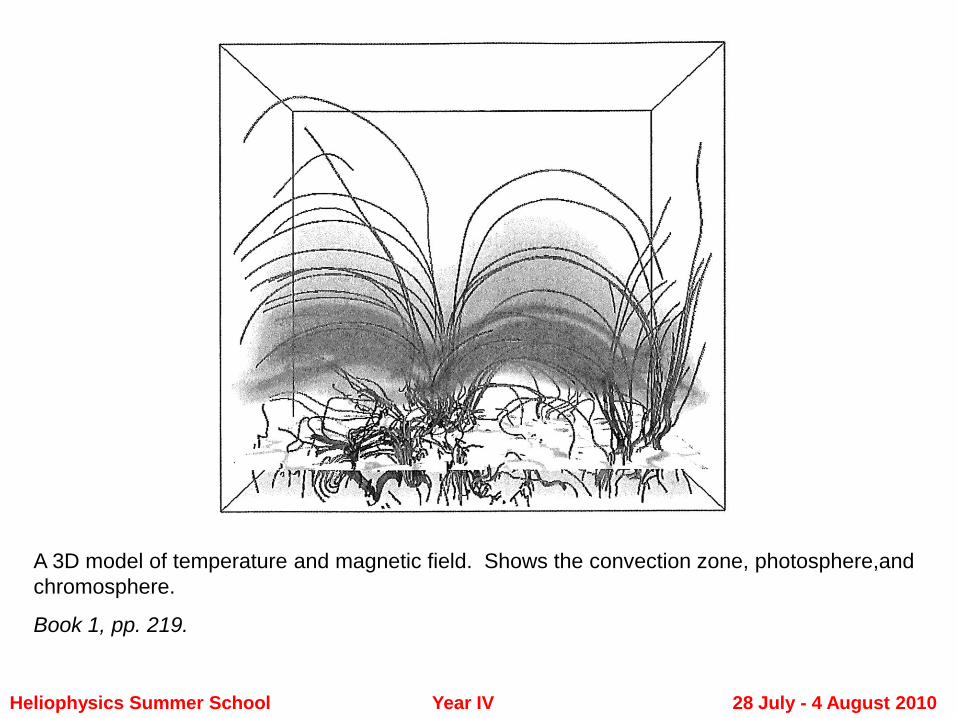
A 3D model of temperature and magnetic field. Shows the convection zone, photosphere,and
chromosphere.
Book 1, pp. 219.
Heliophysics Summer School Year IV 28 July - 4 August 2010
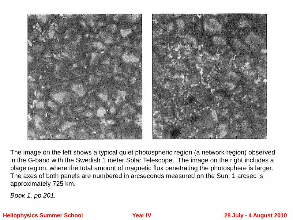
The image on the left shows a typical quiet photospheric region (a network region) observed
in the G-band with the Swedish 1 meter Solar Telescope. The image on the right includes a
plage region, where the total amount of magnetic flux penetrating the photosphere is larger.
The axes of both panels are numbered in arcseconds measured on the Sun; 1 arcsec is
approximately 725 km.
Book 1, pp.201.
Heliosphere
• Includes:
Sun
Solar wind
Geospace
Planets & other objects
• It has:
Heliopause
Bow shock
Interstellar wind
Heliophysics Summer School Year IV 28 July - 4 August 2010
Heliophysics Summer School Year IV 28 July - 4 August 2010
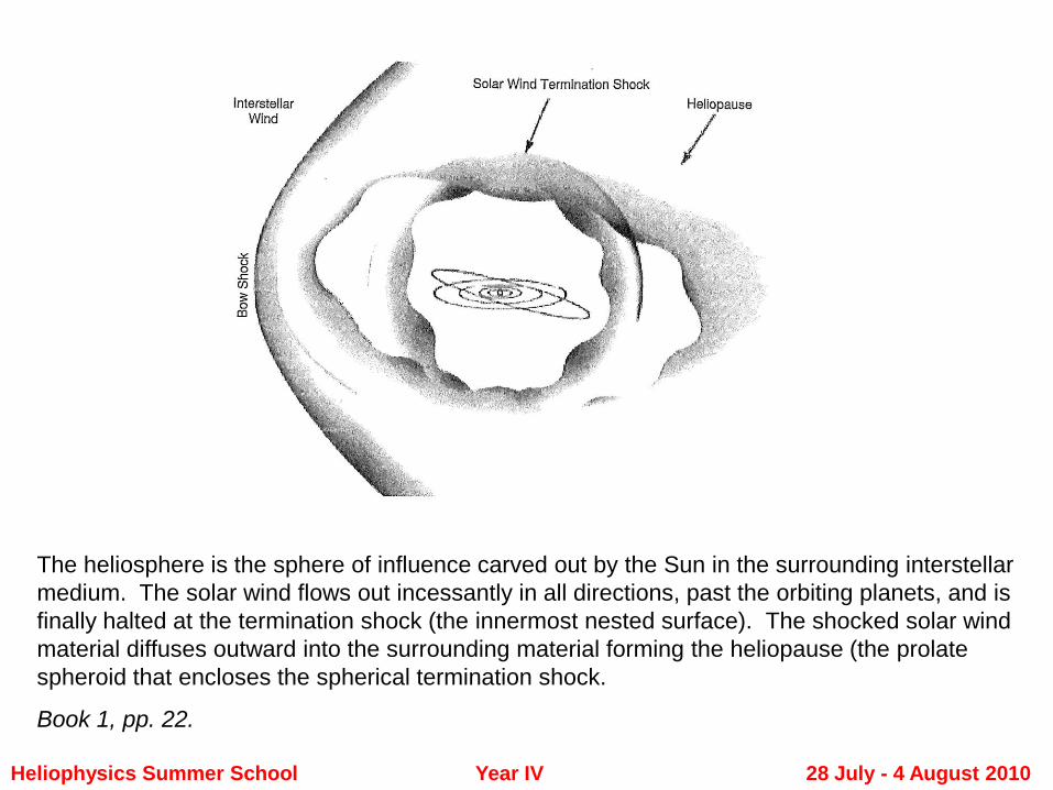
The heliosphere is the sphere of influence carved out by the Sun in the surrounding interstellar
medium. The solar wind flows out incessantly in all directions, past the orbiting planets, and is
finally halted at the termination shock (the innermost nested surface). The shocked solar wind
material diffuses outward into the surrounding material forming the heliopause (the prolate
spheroid that encloses the spherical termination shock.
Book 1, pp. 22.
Heliophysics Summer School Year IV 28 July - 4 August 2010
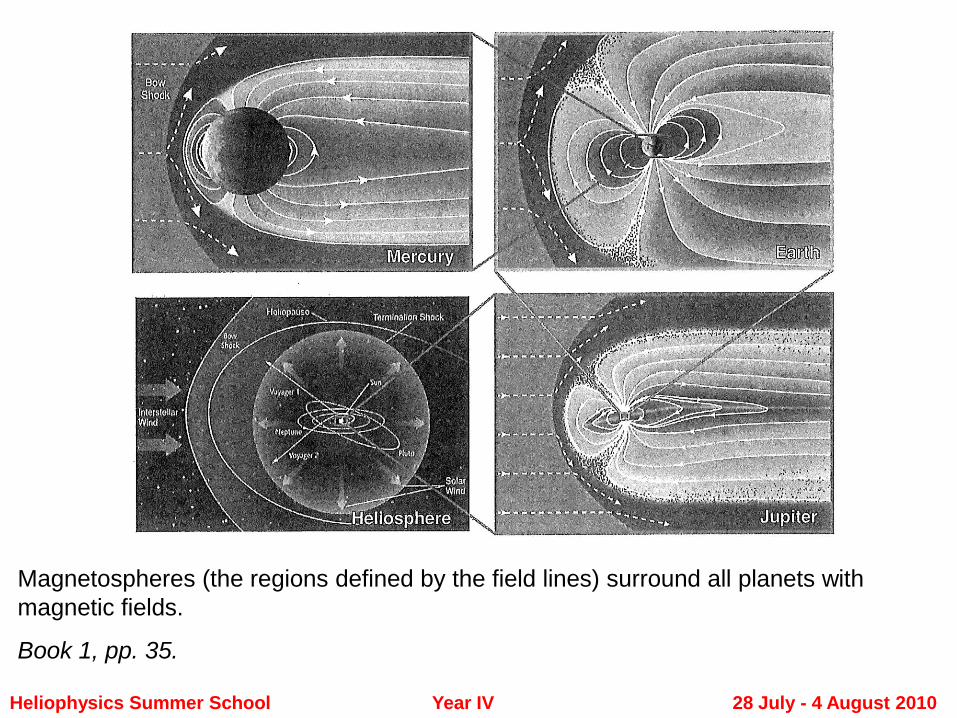
Magnetospheres (the regions defined by the field lines) surround all planets with
magnetic fields.
Book 1, pp. 35.
Heliophysics Summer School Year IV 28 July - 4 August 2010
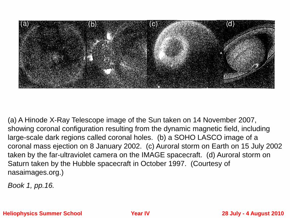
(a) A Hinode X-Ray Telescope image of the Sun taken on 14 November 2007,
showing coronal configuration resulting from the dynamic magnetic field, including
large-scale dark regions called coronal holes. (b) a SOHO LASCO image of a
coronal mass ejection on 8 January 2002. (c) Auroral storm on Earth on 15 July 2002
taken by the far-ultraviolet camera on the IMAGE spacecraft. (d) Auroral storm on
Saturn taken by the Hubble spacecraft in October 1997. (Courtesy of
nasaimages.org.)
Book 1, pp.16.
Heliophysics Summer School Year IV 28 July - 4 August 2010
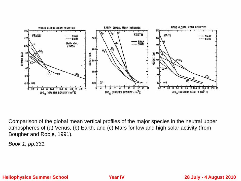
Comparison of the global mean vertical profiles of the major species in the neutral upper
atmospheres of (a) Venus, (b) Earth, and (c) Mars for low and high solar activity (from
Bougher and Roble, 1991).
Book 1, pp.331.
Heliophysics Summer School Year IV 28 July - 4 August 2010
Heliophysics Summer School Year IV 28 July - 4 August 2010