On the Design of Missile Navigation Laws

IntroductionThe set of problems addressed in this note concerns the general rendezvous between two moving objects, so that a certain set of constraints is met at the end of the manoeuvre. The problem has its simplest form when the two objects do not need to match speed at the point of closest approach, this is the case for a missile hitting a target.

The missile steers by generating centripetal forces to change the direction of the velocity vector in space. We shall assume that, from a navigation perspective, these forces can be generated instantaneously. Near intercept, when the time to go approaches the missile response time, this will not be the case, and the effects of the loop delays need to be taken into account. However, as far as the derivation of the fundamental steering algorithms is concerned, this is extraneous detail, which will be visited later.

The problem to be addressed is the derivation of the steering law which will cause the missile to collide with the target. More precisely; we seek to derive a lateral acceleration command from the engagement geometry such that the missile will follow a path which will intercept the target.

First Thoughts

Figure 1 : Sight Line Navigation – Principal Sensor near Launch Point

Perhaps the most obvious trajectory is along the line of sight joining the launch point to the target. As the target moves this sight line direction changes and the missile must manoeuvre to stay on it. Sooner or later the missile will hit the target provided the sight line is known accurately and the missile is able to stay on it. This is the navigation law underpinning beam rider and command to line of sight guidance. Miss distance arises from the kinematic tracking error and system noise, not from the navigation law itself.

Figure 2 : Homing - Principal Sensor on Missile

Line of sight guidance featured widely in first generation guided weapons, and many surprisingly effective systems have employed it, but it is restricted by sensor noise to relatively short ranges, and has typically inferior performance against crossing targets compared with other options.

HomingRather than place the sensor on the launch platform, it may be placed on board the missile. We usually refer to a guidance system which mounts the principal sensor on the missile itself as a ‘homing’ guidance system.

Because the sensor is no longer mounted in an inertial reference frame, its motion affects the navigation, so the ideal behaviour is not as trivially obvious as it is for the line of sight navigation philosophy. The kinematics may be derived from Figure 2.

We consider that homing guidance begins with the missile placed somewhere near the target direction, either by the launch platform, or by a mid-course guidance algorithm designed to (for example) maximise range or minimise time of flight, depending on the engagement conditions. There doesn’t appear to be much point in aiming away from the target. The true motion is in three dimensions, but

the small angle approximations appropriate for Figure 2 permit the vertical and horizontal motions to be treated separately. Cluttering the equations with extraneous detail hardly serves our purpose in imparting understanding.

The earliest attempts at homing guidance followed the philosophy of line of sight guidance and sought to point the missile velocity vector along the sight line from the missile to the target. Like the surface-based line of sight guidance it was reasoned that sooner or later the missile must hit the target. We shall examine this assertion. We shall assume a constant velocity target and constant speed missile, i.e. the target speed and direction are both fixed, but the missile may change its direction of flight.

The navigation law (called ‘pursuit’) generates an acceleration command (fy) proportional to the difference between the missile heading γ and the sight line direction φ:

f y=k p ( γ−ϕ )

Where kp is the pursuit gain. The lateral acceleration is equal to the centripetal acceleration:

f y=Um γ

Differentiating the navigation law, we can eliminate the heading angle:

˙f y=k p ( γ−ϕ )=k p( f y

U m−ϕ )

Sightline KinematicsFrom Figure 2, the sight line direction is given by:

yT− ym=Rϕ

Differentiating once:

yT− ym=R ϕ+R ϕ

And again:

yT− ym=R ϕ+2 R ϕ+R ϕ

The constant speed and small angles assumption means:

yT ≈0 , R ≈0 , ym≈ f y

So the sight line kinematics are governed by:

f y=−2 R ϕ−R ϕ=2U c ϕ−R ϕ

Where UC is the closing speed along the sight line.

Evidently, the sight line direction does not appear in the governing equation, only its rate of change is present. The slew rate of the sight line is traditionally called the ‘sightline spin rate’, for reasons nobody has ever explained to me. We shall denote it ω. Its significance may be understood by considering what the miss distance (xm) would be if the missile did not alter its current heading. This is usually called the ‘zero effort miss’, and is sometimes abbreviated to ‘ZEM’ by those who take delight in obfuscation.

xm ≈ yT− ym+ RU c

( yT− ym )=Rϕ+ RU c

( Rω−U c ϕ)= R2

U cω

The sight line spin rate is therefore an estimator of the predicted miss distance, which is why it is important in considering homing navigation laws.

When the sight line spin is zero, the sight line direction in space remains constant, and the missile closes in on a constant bearing course.

We may write the sight line equations in terms of the predicted miss distance, which is the quantity we actually wish to reduce to zero by the time we reach the target.

We have:

ω=U c

R2xm , ϕ=

U c

R2 xm+2U c2

R3 xm

Substituting in the sight line kinematics equation:

f y=−U c

Rxm

This is interesting. The rate of change of predicted miss distance is proportional to the lateral acceleration. So if we made the lateral acceleration proportional to the predicted miss distance, the navigation law will tend to reduce the miss distance as it approaches the target. We shall return to this point later.

Pursuit AnalysisThe pursuit navigation law, in terms of predicted miss, becomes:

ddt (−U c

Rxm)=k p(−U c

U m Rxm−

U c

R2 xm)As kp→∞, the left hand side of this expression becomes negligible, so the miss distance is characterised by:

xm+U m

Rxm=0

Note: kp→∞ has the same effect as maintaining γ=φ, i.e. the missile velocity vector always points along the sight line.

If the initial time to intercept is T, the time to intercept at time t is (T-t). In other words:

R=U c (T−t )

The miss distance equation becomes:

(T−t ) xm+Um

U cxm=0

This has a solution of the form:

xm=(T−tT )

n

xm0

Where xm0 is the initial miss distance.

xm=−n (T−t )n−1

T n xm 0

From which:

n=U m

U c

This is positive, so it looks like the miss distance reduces to zero, and pursuit appears to work.

However, that is not the full story. The lateral acceleration is given by:

f y=−1

(T−t )xm=n (T−t )n−2

T n xm0

This means that the lateral acceleration requirement increases without bound unless:

Um

U c>2

This can only happen in a tail chase for which Uc≈Um-UT. The infinite lateral acceleration will not be encountered if:

Um<2UT

If the missile speed is higher than this, the controls will saturate, but obviously it cannot be less than the target speed, or it could never catch the target.

The collision course, which is finally reached at intercept , is along the target velocity vector.

Pursuit guidance was used in the first air-to-air missiles for which a tail chase was the only feasible direction of attack because the insensitive infra-red sensors of the time relied on detection of the hot jet pipe of the target, and had negligible forward hemisphere coverage. Pursuit, combined with an insensitive detector, appears to offer a simple synergetic solution.

Curiously, pursuit is nowadays restricted to attacking stationary targets for which the ratio of missile speed to closing speed is unity, which is well below the ratio required to avoid control saturation.

Proportional NavigationWe noted from the sightline kinematics that sight line spin is an estimator of the miss distance. Also the rate of change of miss distance is proportional to the lateral acceleration. Thus by setting the lateral acceleration proportional to the sight line spin, the missile should steer so as to reduce the miss distance to zero.

The behaviour we want is characterised by miss distance reducing with time to go, e.g:

xm=(T− tT )

N

xm0

This implies a navigation law of the form:

xm=−N (T−tT )

N−1 xm0

T= −N

(T− t )xm

Now:

xm=− (T−t ) f y , xm=U c (T−t )2ω

In terms of lateral acceleration and sight line spin:

f y=N U c ω

This is known as proportional navigation. N is called the navigation constant.

Comparing the equation of motion with that for pursuit, we see the N replaces Um/Uc, so to avoid saturation; N >2.

However, the value of N is not constrained by the missile and target speeds, so the N>2 criterion can be met for engagements at any aspect, not just a tail chase. For this reason, proportional navigation has largely supplanted pursuit.

Choice of Navigation ConstantThere are two long-standing erroneous assertions regarding homing, which have become part of the folklore. These myths need to be dispelled.

The first is the assertion that pursuit is proportional navigation with a navigation constant of unity. As is shown in the previous section the effective navigation constant is Um/Uc, which is unity only if the target is stationary. Provided the target is engaged in a tail chase with missile speed less than twice the target speed, pursuit does not necessarily lead to control saturation, as appears to be almost universally believed.

The other is the claim that a navigation constant of 3 is optimal.

The value of 3 is derived from minimising a performance index which amounts to the integral of the induced drag over the engagement, i.e. the integral of the square of the lateral acceleration over the flight. The figure of 3 arises for no reason other than a quadratic index is used. However a quadratic performance index is used solely for mathematical convenience, it has no other significance. It would be equally legitimate to use an index of the form:

L=∫ f y2n dt

Where n is a positive integer. Optimising the problem to minimise this performance index leads to the result that the ‘optimum’ navigation constant is:

N= 4n−12n−1

When n=1, as in the (ad nauseum) quoted result, the ‘optimum’ navigation constant is 3. As n→∞, the navigation constant tends to 2, the significance of which we have already found as the lower limit of navigation constant before control saturation sets in.

The value of three is an artefact of the somewhat arbitrary choice of the power of 2 in the performance index, it has neither physical nor operational significance.

Indeed, in the stage of the engagement when the aiming error needs to be removed, the missile is close enough to the target for energy loss due to induced drag to be the least of our worries, so optimising the navigation law on the basis of a performance index which bears no practical relevance to the problem seems a spurious exercise. It is the kind of result we expect when those who understand the problem don’t understand the maths, and those who understand the maths don’t understand the problem.

With the ever wider gulf between the geeks and the poseurs, which characterises modern engineering, this problem is expected to worsen.

Less spurious work, undertaken in the early 1960s by Cornford and Bain, recognised that, as the time to go approached the response time of the missile, the guidance loop would tend to instability. Using this criterion, which has the merit of actual relevance to the problem, a navigation constant of 4 was deemed ‘optimum’.

The choice of navigation constant depends on the stage of flight. For the mid-course, if no other criteria apply (which is unlikely to be the case), the value of between 2 and 3 might be relevant, but towards the end, the stability criterion is expected to dominate, and a value closer to 4 is to be expected.

We can understand the effect of navigation constant by considering the miss distance half way through the flight:

xm2=( 12 )N

xm0

Values of miss distance at the half way point are presented in Table 1. The higher the navigation constant, the quicker the missile settles on to the collision course.

N Xm2

2 0.253 0.1254 0.06255 0.03125

Table 1: Effect of Navigation Constant

Evidently, the higher the navigation constant, the sooner the missile approaches the constant bearing collision course, which it only reaches exactly at intercept.

The implication is, the higher the confidence in the predicted impact point, the higher the value of navigation constant which can be used. Sensor noise and target manoeuvre are expected to dictate the upper bound, not some naive optimisation exercise. At close range there is less chance for the target manoeuvre, and it is reasonable to assume the noise is reduced for a sensor mounted on the missile, so the stability-based criterion will probably set the upper bound on navigation constant.

In practice, extensive modelling is undertaken to optimise the navigation constant at different stages of flight, based on the actual constraints of the engagement, although a value between 3 and 4 is usually a reasonable first iteration.

Further ConsiderationsThe sight line spin rate needed for proportional navigation is measured with respect to an inertial datum (represented by the initial aim direction, which is fixed in space). It is not simply the rate of change of the look angle (nowadays somewhat pretentiously called the ‘angle of regard’). Also, an estimate of the closing speed is required, although this does not need to be particularly accurate.

Sensors which can achieve this are invariably expensive, which is unfortunate considering they are expended with the round, but that is the penalty for requiring all aspect coverage. A much cheaper round could be used by engaging the target in a tail chase by launching from an unmanned vehicle

manoeuvred into the enemy tail cone region and using pursuit guidance in the actual round. Such vehicles could be operated as a defensive fence on patrol around the perimeter of the defended area.

It is interesting to speculate whether there is any mileage in using rate of change of look angle, rather than sight line spin as a potential guidance law.

In its ideal form, the guidance law would be expressed as:

f y=k v ( γ−ϕ )

This is the same expression as was used to derive pursuit guidance, so we should expect the same kinematic limitation. This analysis is insufficient to resolve any difference between this algorithm and ordinary pursuit. In practice, we should aim to broaden the cone of coverage around the target tail as far as possible by designing a PID controller with look angle as input.

Integrated Proportional Navigation The fact that pursuit furnishes a solution to the miss distance equation implies that under certain conditions the look angle itself can be an adequate estimator of the sight line spin rate, and therefore an estimator of the miss distance. The sight line kinematic equation is:

f T−f y=−2Uc ω+R ω

With no target acceleration, this becomes:

−Um γ=−2U c ω+R ω

Or: −Um γ +U c φ=R φ+R φ

Integrating:

U c φ−U mγ=R φ+c

Where c is a constant.

If we have an independent measure of the heading, this may take the form:

U c ( φ−γ )+(U c−U m )γ=R φ+c

Taking the initial aim direction as the reference, the constant ‘c ‘ is found as:

c=U c φ0−Ro φ0

Where the subscript 0 denotes the initial conditions. This constant would be generated by the launch platform from the current engagement conditions.

Using the look angle, and an estimate of heading, the sight line spin rate may be estimated. This could then be used in a proportional navigation guidance law to steer the missile.

More General End Game ConditionsIn some applications hitting the target is not sufficient. The warhead may be designed for an optimum direction of approach, so that there is a need to control the terminal flight path direction, as well as miss distance. This is also the approach needed for rendezvous, rather than intercept, with the target.

Lead PursuitWe noticed with pursuit guidance that for any aspect other than near tail-on the control would most likely saturate. If we modify the law by placing a bias on the look angle, i.e.:

f y=k p ( γ−ϕ+ϕ L)

We do not modify the analysis, but the collision course, rather than about the target velocity vector, is with respect to the collision course corresponding to the look angle φL, usually called the lead angle. The kinematic constraint of the ratio of missile to target speeds still applies, so only rear hemisphere coverage is possible, but this scheme broadens the engagement cone considerably. It is known as ‘lead pursuit’, and was introduced to improve basic pursuit, but has been largely abandoned in favour of proportional navigation.

Terminal Heading ControlIf we wish to control both miss distance and terminal direction of approach it appears we need feedback of both heading and miss distance:

f y=k γ ( γ D−γ )+km xm

Now, the lateral acceleration could become zero with the heading error term and miss distance term simply being equal and opposite, whilst both actually diverge from the desired end state. Rather than both being reduced to zero, they become equal and opposite and neither guidance objective is met.

Liapunov ApproachIn order to avoid the possibility that the errors in the two states being controlled could become equal and opposite, we deal with a quantity which is always positive regardless of the signs of the two errors.

What is needed is a control for which the quantity:

V=bγ ( γ D−γ )2+bm (T−t )2ω2+b3 (( γD−γ )+ β (T−t )ω )2

Where b¥ , bm and b3 are positive constants, reduces to zero at intercept . The time to go is included to ensure that these have the same dimensions. This approach is known as Liapunov’s direct method, after one of the early pioneers of control theory.

This tends to zero as t→T. In other words:

V <0

For all values of miss distance and heading error.

The Liapunov function, V may be written more compactly in matrix form:

V=( ( γ D−γ ) (T−t )ω )(b11 b12b12 b22)( ( γ D−γ )

(T−t )ω)=xT Bx

Where the matrix B is symmetric and positive definite, i.e:

b11>0

b11b22−b122 >0

The time derivative is:

V= xT Bx+xT B x

Since B is symmetric:

xT Bx=xT B x

So: V=2xT B x

From the system kinematics:

x=( −γ−ω+ (T−t ) ω)=(

−f y

Um

−f y

U c+ω)

The presence of the additional ω term is an inconvenience as it gives rise to a term:

X=b12 ( γ D−γ ) ω+b22 (T−t ) ω2

It doesn’t seem likely that this term will be negative definite. Our experience with homing guidance so far indicates that some form of modified proportional navigation is in order:

f y=N U c ω+k v ( γ D−γ )

Evidently, if N>1 the additional ω term will not change the sign of the lateral acceleration term. By taking a control law of this form we can eliminate the inconvenient extra term.

The derivative is the sum of four terms:

V 1=−b11f y

U m( γ D−γ )=−b11(N

U c

Umω ( γ D−γ )+

kv

Um(γ D−γ )2)

V 2=−b12( f y

U c−ω)( γ D−γ )=−b12( ( N−1 ) ω ( γ D−γ )+

kv

U c( γD−γ )2)

V 3=−b12f y

Um(T−t ) ω=−b12(N

U c

U m(T−t )ω2+

kv

U m(T−t ) ( γ D−γ ) ω)

V 4=−b22( f y

U c−ω) (T−t )ω=−b22( ( N−1 ) (T−t )ω2+

kv

U cω (T−t ) ( γ D−γ ))

We can ensure the derivative is negative definite by eliminating the cross-products of heading error and sight line spin:

( N−1 )b12=−NU c

Umb11

k v

U mb12=

−kv

U cb22⇒b12=

−Um

U cb22

So that: b22=N

N −1 (Um

U c)2

b11

Positive definiteness requires:

b11b22−b122 =b11

2 ( NN−1 (Um

U c )2

−( NN−1 )

2

( U c

Um )2

)>0This is impossible to achieve, except perhaps in a tail chase.

It certainly cannot be achieved against a stationary target. The alternative to expressing the derivative in terms of a sum of squares is to express it as the negative of a squared quantity. The presence of the time to go in the cross product terms implies the navigation law should be modified such that:

k v=gv

T−t

The derivative now becomes:

V 1=−b11(NU c

Umω ( γ D−γ )+

gv

Um (T− t )2( γ D−γ )2)

V 2=−b12(( N−1 ) ω ( γ D−γ )+gv

U c (T−t )2(γ D−γ )2)

V 3=−b12(NU c

Um(T−t ) ω2+

gv

Um(γ D−γ ) ω)

V 4=−b22(( N−1 ) (T− t ) ω2+gv

U cω ( γ D−γ ))

We could try re-arranging until we get a function which is negative definite (e.g. a perfect square), but it is probably easier to investigate the solution explicitly, using the feedback law derived from the constraints identified by the Liapunov function.

Explicit SolutionThe governing equation is:

f y=N U c ω+gv

(T−t ) (γ D−γ )

Including the sight line kinematics:

2U c ω−(T−t ) U c ω=N U c ω+gv

(T−t ) (γ D−γ )

Or: (T−t )2U c ω+ (N−2 ) U c (T−t ) ω=−gv (γ D−γ )

Differentiating:

(T−t )2U c ω+ (N−4 ) (T−t ) U c ω−(N−2 ) U c ω=gv γ=gv

U mf y

Let: β=gv

Um, so that the governing equation becomes:

(T−t )2ω+( N−4+β ) (T−t )ω−(2 β+N−2 ) ω=0

The solution is expected to be of the form:

ω=a (T−t )n , ω=−an (T−t )n−1 , ω=an (n−1 ) (T−t )n−2

These substitutions reduce the differential equation to an algebraic equation in n:

n (n−1 )−n ( N−4+ β )−(2β+N−2 )=0

Both roots must be positive, otherwise the solution will diverge. This means β must be negative, and:

|β|> N2

−1

The solution for n becomes:

n=12 ( ( N−3−β ) ±√( N−3−β )2−4 (2 β−( N−2 ) ))

When

|β|=N2

−1

n=0 ,∨n= N2

−2

Which implies the navigation constant must be 4 or greater.

CommentThe control of final dive angle is important when the target has a vulnerable direction of attack, or the warhead is directional and only effective at a particular impact angle. Also, when engaging a sea-skimming missile it may be necessary for the terminal trajectory to consist of a dive at the Brewster angle to minimise the effect of reflections from the sea surface.

Not surprisingly, it is harder to simultaneously meet a terminal constraint and also hit the target, than it is just to hit the target. High values of navigation constant are required, which implies sensitivity to system noise and missile lags. We should not expect to achieve the same miss distance performance as is achievable without the terminal constraint. Trade-offs are required, which are specific to the system under investigation and way beyond the scope of this note.

Effect of AccelerationThe assumption has been that the missile speed is constant, and the target does not manoeuvre. In general the target has its own mission to conduct and will usually only manoeuvre if it believes itself to be under threat. We should expect the target’s own mission to be compromised by having to manoeuvre.

Consider first the case of an accelerating missile. Assume a constant tangential acceleration ‘fx’. The left hand side of the sight line kinematic equation becomes;

− y=−f y−f x γ

The sight line acceleration term on the right hand side is no longer zero:

R φ=−f x φ

We see the immediate effect of the longitudinal acceleration is to introduce an additional acceleration term:

− y−R φ=− f y +f x (φ−γ )

The immediate effect of the acceleration is to introduce a term proportional to the look angle. It is common practice to measure this term and subtract it from the guidance command; a technique known as ‘longax compensation’.

With this compensation, the sight line equation becomes:

−f y=2 R φ+R φ .

The range is given by:

R=R0−U0 t−12

f x t 2

Where R0 is the initial range, U0 the initial closing speed and t is time from launch. Differentiating:

R=−U0−f x t

Expressing this in terms of time to go:

R=R0−U0 (T− tgo )−12 f x (T−tgo )2=U0T +12

f x T 2−U 0 (T−tgo )−12 f x T 2+f x Tt go−12

f x t go2

Where T is the time of flight from launch.

The range to go becomes:

R=(U0+ f x T ) (T− t )− 12

f x (T−t )2

The closing speed is, similarly:

R=−(U0+f x T )+ f x (T−t )

The sight line kinematics equation, excluding the longax compensation becomes:

−f y=2[−(U 0+ f x T )+ 12 f x (T−t )]ω−f x (T−t )ω−[[−(U 0+ f x T )+ 12 f x (T−t )] (T−t )] ω

This suggests a navigation law of the form:

f y=−NU 0 [−(1+ f x

U0T )+ f x

2U 0(T−t )]ω

The equation of motion becomes:

( N−2 )U0ω+(T−t ) ω=fn (T−t ) ω

Where fn is used to denote that the coefficient of ω on the right hand side is a function of the time to go.

There might be a general analytic solution to this. I will leave that to people who don’t get out much.

Practical ConstraintsMissiles are usually solid-fuel rocket-propelled, and therefore unlikely to maintain constant speed throughout the flight. The initial boost phase to accelerate the missile to its nominal speed can introduce considerable aiming error if the longax compensation is omitted. However, the slow/down or acceleration in the sustain phase is not expected to be large and:

f x TU0

<<1

As a first iteration at least, the effect of longitudinal acceleration during sustain can be ignored, and the problem treated as ordinary proportional navigation. The value of longax compensation during the sustain or coast phases becomes questionable when the measurement errors associated with it are taken into account.

At the other extreme the missile may be accelerating throughout the engagement, as could be the case with an endo-atmosphere anti-ballistic missile. For reasons which should be obvious, these will not be discussed.

Target AccelerationAs already mentioned, the target has troubles of its own. It is only there to perform some kind of mischief, and it is the responsibility of the missile to put a stop to it. Unless the target believes it is being attacked, it will generally fly straight and level. It is therefore of paramount importance for the missile to approach to within a no-escape range before it is detected. This is practically impossible to achieve.

Homing sensors fall into three basic categories:

Passive Semi-active Active

Passive sensors rely on the emissions from the target. They could be the target’s own sensor emissions, as in the case of an anti-radiation missile, designed specifically to destroy sensors, or it could be infra-

red, visual band or ultra-violet emissions. These give little or no warning from the sensor, but with the exception of ARMs, tend to be short range, so the target is usually close enough to see the missile launch.

Semi-active uses an illumination from a separate source, typically the launch platform. The missile detects the reflections from the target. The switching on of the illuminator clearly gives warning of the presence of a threat, and usually an indication of its expected direction.

Active uses a sensor which carries its own energy source. Since the missile is unlikely to generate much power within itself, the active seeker is not usually switched on until the end game, with the missile command-guided from launch to the acquisition range. Once the seeker starts to emit it becomes detectable.

Any legitimate military target, more likely than not, is expected to have the ability to sense when it is in immediate danger, and is expected to take evasive action. The use of sophisticated weapons against non-military targets is an intolerable affront to the honourable profession of arms.

It is reasonable to believe that the target is very likely to manoeuvre in the end game. The effect of this can be found by including target manoeuvre in the sight line kinematics:

ω+( N−2 )(T−t )

ω=f T

U c (T−t )

Multiply both sides by:

( T−tT )

− ( N−2 )

The sight line equation reduces to:

ddt (ω( T−t

T )−( N−2 ))= f T

Uc

(T−t )−( N −1 )

T−( N−2 )

Which, on integrating, yields the sight line spin due to target manoeuvre:

ω= 1( N−2 )

f T

U c(1−(T−t

T )( N −2 ))

The higher the navigation constant, the more robust the guidance is to target manoeuvre. Note that the ‘optimum’ value of 3 is not particularly effective at reducing the sight line spin due to target manoeuvre. The lateral acceleration required becomes:

f y=N

N−2f T (1−( T−t

T )( N−2 ))

The acceleration advantage required of the missile over the target increases without bound as N reduces to 2. Evidently, the navigation constant must be as large as possible to minimise the effect of target manoeuvre. The ‘optimal’ value of 3 appears to require an advantage of 3:1.

We cannot increase the navigation constant indefinitely, because we will run into noise, saturation and end game stability problems, so if the maximum navigation constant we can use still results in excessive miss distance, we need to think of an alternative.

In the presence of target acceleration the zero-effort miss becomes:

xm=( yT− ym )+( yT− ym ) (T−t )+ 12 ( yT− ym ) (T−t )2

Substituting from the sight line equations:

xm=Rφ+ RU c

(−U c φ+R φ )+ 12 ( RU c )

2

(−2U c φ+R φ )

xm=12 ( R3

U c2 ) φ

As before, we design our navigation law such that:

xm=−Nxm

(T−t )

Now:

xm=32

R2 RU c2 φ+1

2R3

U c2 φ

The third derivative requires us to differentiate the sight line kinematics equation:

− f y=−2U c φ+ R φ+R φ=−3U c φ+R φ

φ=3U c φ− f y

R

Hence:xm=− 1

2 ( RU c )

2f y

From which we conclude the navigation law is of the form:

f y=NU c φ

This appears to be proportional navigation differentiated. However, the integral introduces a constant:

f y=NU c φ+const

The sight line kinematic equation will reduce to proportional navigation if:

const=f T

The navigation law consists of proportional navigation with an estimate of target acceleration added in.

The filters used to estimate target acceleration on board the missile typically measure the missile acceleration using an accelerometer, and use a state-space formulation of the sight line kinematics:

^ω=2U c

Rω+1

Rf T+kω ( ω−ω)−1

Rf y

^f T=k f (ω−ω)

Where the hat is used to denote an estimated quantity and kω, ,kf are (usually time-varying) gains.

In principle, the target acceleration could be estimated by the launch platform and communicated to the missile.

However, whether the error in estimating the target acceleration is less than the kinematic miss caused by leaving it out is very much a matter for detailed analysis of the specific system under consideration, and lies outside the scope of this note.

A Different PerspectiveThe more astute will have noticed that in solving terminal controller problems the term (t-T)n is analogous to the e-at term of constant coefficient linear homogenous differential equations. Using this substitution in the time-varying equations yields a characteristic equation from which the exponent can be calculated.

However, there is no equivalent to the frequency domain description of the system which would justify using a Laplace transform to concatenate elements together into a more sophisticated controller. We must perform all the necessary algebraic manipulation explicitly.

In order to consider the effect of concatenating two or more time-varying blocks, we need a description which is analogous to the Laplace transform.

The simplest approach is to convert the time-varying equations into constant coefficient equations. Considering the form of the solutions of these two types of equations, we should expect a substitution of the form:

τ=−ln (T−tT )

Would do the trick.

Differentiating, we find:

dfdt

=dτdt

dfdτ

= 1(T−t )

dfdτ

Applying this to the basic PN homing equation:

( N−2 )ω+(T−t )ω=0

This becomes:

( N−2 )ω+ dωdτ

=0

This is now a constant coefficient equation, to which we can apply Laplace transforms to analyse. We shall use D to denote the Laplace Transform associated with τ, to avoid confusion with the usual ‘s’ which is associated with actual time.

The PN equation with the target acceleration compensation in place becomes:

f T−NU c ω− f T=−2U c ω+U c (T−t ) ω

The guidance filter equation is, ignoring missile autopilot lag:

^ω=(2−N )U c

Rω+kω

U c

R(ω−ω)

^f T=k f

Uc2

R(ω−ω)

Using our understanding of the basic homing equation, we have modified the filter gains so that they become pure numbers. The overall system equations are now:

(T−t ) ω=2ω−N ω−1Uc

f T +1Uc

f T

(T−t ) ^ω=(2−N−kω ) ω+kωω1U c

(T−t ) ^f =k f ω−k f ω

Or, in terms of our Laplace-like operator:

(( D−2 ) N 1U c

−kω (D+k ω+N−2 ) 0

−k f k f1

U cD )(ω

ωf T

)=(1

U c

00

) f T

The true sightline spin rate is our measure of guidance performance, whether the missile is accelerating or not, because when it is zero, there is no relative motion perpendicular to the line of sight. The effectiveness of the target acceleration estimation is therefore determined by the pseudo transfer function:

ωf T

=G ( D )

From the final value theorem, the condition at intercept is given by:

D G (D )D→0

If fT is constant, then in the transform domain it becomes:

f T (D )=f y

D

So the final value of the sight line spin is just equal to the transfer function as D→0. The denominator of the transfer function becomes the constant term of the characteristic equation, i.e. the determinant of the matrix of coefficients:

Δ (0 )=|−2 N 1

Uc

−kω (k ω+N−2) 0−k f k f 0

|=k f( N−2 )

Uc

The numerator becomes:

ω (0 ) Δ (0 )=|

1U c

N 1U c

0 (kω+N−2 ) 00 k f 0

|=0

So, as expected, the sight line spin is indeed reduced to zero as the target is approached.

Also, the ‘steady state’ target acceleration estimate is:

f T (0 ) Δ (0 )=|−2 N 1

U c

−k ω (kω+ N−2 ) 0−kf kk 0

|=k f( N−2 )

U c

The final missile acceleration is equal to the target acceleration, implying the manoeuvre capability may be much lower than is required for basic proportional navigation.

Figure 3 : Homing Loop with Target Acceleration Estimation

Well, hooray; all we have done is demonstrated what we already knew, that the target acceleration estimator does indeed work. The exercise does not seem to have yielded insight commensurate with the effort involved.

As in most modern matrix-based approaches, the topology of the system from which most of its properties may be understood, is conspicuous by its absence. If we sketch the loop as in Figure 3, we see that the acceleration estimator in fact introduces integral of error into the guidance loop. This now makes sense from a control perspective, and explains why a large loop gain (navigation constant) is not needed. Integral feedback is a standard trick used to improve the tracking properties of a control loop.

Concluding CommentsDoubtless this note will attract the criticism that it is ‘ad hoc’. Actually, ‘ad hoc’ is a term frequently used by mathematicians and others whose understanding of the problem is very narrow in scope. More often than not the problem is no more than a means of illustrating a technique, rather than discovering how a real world entity behaves.

All too often I come across text books allegedly written ‘for engineers’ which appear to be based on the patronising assumption that engineers are merely inferior mathematicians who need to be given methods which can be blindly handle-cranked to produce solutions, with no real understanding of the process involved. The entire edifice is usually based on a naive one-dimensional criterion, which may or may not have any relevance to the problem, whilst in fact the problem is multi-dimensional, and requires ingenuity, creativity and domain knowledge to resolve.

In contrast, the engineer brings his/her wide experience and broad understanding to bear on the problem, identifying simplifications which arise from understanding of the processes involved, and therefore opaque to those whose knowledge is blinkered.

The equations may be derived more rigorously without the small angle approximations. However, they would take up much more space but add very little to the understanding of the basic principles. The more exact kinematics would be included in a model, when precise answers for specific systems are being sought, but most actual insight is furnished by the linear analysis.

Nothing in this note can be applied directly to any real system much beyond the initial concept stage. Performance calculations based on such a high level analysis will be wildly optimistic. It takes considerable knowledge and experience to take these almost philosophical assertions and produce a viable weapon system.

In systems work, we seem to confuse ‘top level’ with ‘merely shallow’, the vague, the bland and the turgid seem to have ousted the concise and quantitative. What is actually required is a system characterisation of the level presented here which enables us to say definite things about how it behaves ideally, before introducing the myriad of real world effects which prevent the ideal behaviour from being achieved.

If we don’t have an understanding of the system behaviour in its ideal state as a starting point, we really are on the high road to nowhere.

Line of Sight Guidance

IntroductionMost first generation missiles employed command guidance of some form or other. Using the sensors of the time it was not possible to observe the three dimensional position errors between missile and target accurately enough to achieve small miss distances. The line of sight geometry required just the two lateral position errors to be known, which was feasible with the trackers of the time, notably the human eyeball.

Also, the line of sight geometry was a natural development of the gun systems which were prevalent at the time. Furthermore, the early infra red seekers could only detect the hot jet pipe of the aircraft, and so could only engage after the enemy has over flown the target and done its mischief.

Line of sight guidance has been used in air to surface and surface to surface (anti-tank), but predominantly it is used in surface to air weapon systems. With improvements in seeker technology, it is likely to be abandoned in this role as well.

It has the advantage of a relatively low cost round, as most of the expense is concentrated in the platform sensors and launcher/magazine systems.

In the surface to air role, the object of the exercise is to defend a region about the launch point.

Figure 4 : Coverage Characterisation

We define the performance of a surface to air system in terms of the volume of space it denies to the enemy. To begin with, at least, we treat the target as a constant velocity point. Once we have gained understanding of the constraints under these simple conditions, we may proceed to more complex target behaviour.

The coverage is referred to an axis with missile launch point as origin, with x-axis parallel but in the opposite sense to, the incoming threat. This is the ‘forward range’ axis. Perpendicular to this axis is the ‘crossing range’ axis. Using this as the reference set it is reasonably easy to determine the constraints which limit coverage capability.

Constraints

Kinematic

Figure 5 : Engagement Kinematics

The kinematics of the engagement are presented in Figure 5. Unless both target and launch platform are stationary, the missile velocity vector will not be aligned with the sight line. This immediately imposes a constraint, because the angle between the missile velocity vector and the sight line cannot exceed the beam width of the rearward facing sensors of a beam rider or the command link beam width of a command system. These angles will be small primarily to prevent jamming, and in the case of the beam rider to ensure guidance accuracy.

At this level of coarse analysis, we treat the velocity vector as coincident with the body longitudinal axis, so we refer to angle β in Figure 5 as the ‘body to beam’ angle. It is given by:

sin β= RUm

θ

Denoting the instantaneous range from launch point to target RT, we have for the angular velocity of the beam:

θ=U T

RTsin θ

At intercept, R=RT, so we have:

sin β=UT

Umsin θ

It follows that to avoid this constraint, the missile speed must be considerably greater than the target speed. A body to beam limit of about 5 degrees implies a 10:1 speed advantage of missile over target, which for an air target, is out of the question, but could be achieved with an anti-armour missile. Every line of sight guided surface to air missile is therefore expected to run into body to beam angle limitations, which will limit the crossing range cover.

The other pure kinematic constraint is the lateral acceleration requirement. Unlike a homing missile which flies more or less toward the intercept point, the line of sight missile must apply lateral acceleration just to stay on the beam. Since the body to beam angle must be small, for the reasons given, the body lateral acceleration may be taken as equal to the beam lateral acceleration.

f y=2Um θ+R θ

Before considering the feedback control to maintain the missile on the beam it is advisable to include this as a feed forward acceleration into the guidance loop. Note however, this information is not available to a beam rider as it is estimated at the launch platform. Also, it is often difficult to obtain an accurate, noise free estimate of the sight line acceleration and the error in estimating it can easily exceed the miss distance caused by ignoring it, so it is frequently ignored. It is probably better to include integral of error feedback within the loop to eliminate an acceleration bias.

The dominant term in the feed forward is the Coriolis acceleration. This increases as the crossing range reduces, and is a maximum near the crossing range axis.

Additional ConstraintsThe maximum range depends on many factors, but hopefully it will be specified as an input to the analysis process, presumably from higher level tactical studies, based on how far away from the target area the enemy must be kept.

For example, a ground attack aircraft can toss bomb its target from a range of just over 5km. A UAV fitted with optical sensors is not expected to have a stand-off of greater than between 5 and 10km.

These all lie within the ambit of potential line of sight systems. However, to begin with, all options will be considered, and the study will continue to sufficiently fine resolution to enable a rational basis for down-selection, rather than the geek table, power point and guesswork that seems to be the current fashion.

The missile thrust profile will be chosen such that there is sufficient manoeuvre capability at this maximum range to still hit the target. In some circumstances there may be a constraint on the missile size and weight, such as compatibility with existing magazine handling systems and launchers, or restriction to manual loading, or portability/ logistics constraints in which case maximum range may well be dictated by propulsion constraints, and sensors would be selected to suit.

Sometimes a particular missile may be specified, and work is necessary to determine what the consequences will be on overall system performance of pre-judging the characteristics of such a critical system element.

Minimum range might be dictated by the distance needed to gather into the guidance beam, which depends on the method of launch and the spacing of the launcher and sensor. In extreme cases it may be dictated by warhead safety and arming considerations.

A further issue may arise because the number of fire channels may be limited and the overall time between engaging a target and being ready to engage the next might be greater than the spacing between consecutive targets. The density of the attack expected is another consideration which needs to flow down from higher level considerations.

These issues all interact and need to be addressed for the specific system under consideration, probably requiring several iterations before a viable option is derived, or the data is acquired to form the basis of a worth-while system specification.

Only the kinematic constraints may be considered fundamental. The rest are system-specific.

Lead GuidanceThe kinematic limitations arise from the requirement to fly along a moving beam. If, instead, the missile were guided toward the predicted intercept point, these problems would disappear. However if the intercept point were known with such certainty, there would be no need for a missile at all, as an unguided shell would presumably work just as well.

Placing a lead angle on the beam is expected to reduce the severity of the constraints of flying on a rotating beam. A straight forward extrapolation of the target position is usually defeated by the uncertainty in the intercept position, so the idea of flying to a point part way between the current target position and the predicted impact position has been used on certain systems, which will remain nameless. This is called part lead line of sight guidance. The amount of lead angle is a trade off of body to beam angle, manoeuvre capability and uncertainty in intercept point.

In many cases the best compromise has been found to be with an aim point half way between the current target position and the predicted impact point. This result is fortuitous, and believed to be just a feature of the particular systems studied. However, ‘half-lead guidance’, as it is called, is a term which has found its way into the folk lore, so is worth mentioning for completeness.

In guiding up a line other than the line of sight to the target we might alleviate the manoeuvrability problems, but it introduces problems of its own. We can no longer keep both target and missile in the same beam. Either the beam must be broad enough to encompass both, usually with a degradation in resolution and/or signal to noise ratio, or the missile guidance beam must be separate from the target tracker, and we introduce a whole raft of alignment problems. The misalignment of target and missile sensor introduces a guidance error, known as ‘collimation error’ which can place a further constraint on range.

The use of separate guidance and tracking beams is more frequently associated with beam rider, rather than command to line of sight systems, as body to beam angle must be small to maintain a narrow guidance beam. However, with modern phase-array technology, the possibility of steering the sensor to always point at the launch point appears a viable approach to alleviating the body to beam limitation. Indeed the same technology could be applied to steering the command link antenna of a CLOS (command to line of sight) system.

Commanded Proportional NavigationThe scheduling of lead angle with time to go is likely to be a highly system-specific problem. However, as we have derived proportional navigation as a navigation law for systems in which the principal sensor is carried on the missile, it is interesting to see what kinematic advantage there is to implementing it with a pair of surface based sensors. This type of system is known as ‘three-point’ guidance, and to date at least, it has usually been incapable of achieving adequate miss distances.

Figure 6 : Three Point Guidance

General three point guidance does not necessarily require missile tracking sensor and target tracking sensor to be co-located. This version restricts itself to the angular alignment problem in isolation, before obscuring the issue with position alignment errors.

We see from the geometry of Figure 6 that the sight line direction is given by:

tanφ=RT sin θT−Rm sinθm

RT cosθT−Rm cosθm

The exact expression is likely to get very messy, so we’ll leave that to people who don’t get out much. We will concern ourselves with engagements close to the forward range treat axis. If we can’t hit the target there, then what happens at greater crossing ranges is really of academic interest only.

So using the small angle approximations:

φ≈RT θT−Rmθm

RT −Rm

Differentiating:

φ=( RT θT+RT θT−Rm θm−Rm θm ) (RT−Rm )−(RT θT−Rm θm ) ( RT −Rm )

( RT−Rm )2

φ=RT θT−Rm θm

RT −Rm−

( RT Rm−RT Rm)(RT−Rm)2

(θT−θm )

The missile lateral acceleration command becomes:

f y=N ( RT−Rm ) φ

It appears that proportional navigation does not depend critically on the alignment of the two beams; a fixed collimation error is removed by the process of differentiation.

In three dimensions, the sight line becomes a vector expression:

s=(RT−Rm)|RT−Rm|

Where the underscore denotes a vector quantity and the ‘hat’ in this context denotes a unit vector.

The missile and target lines of sight define a plane having unit normal:

n=RT×Rm

|RT×Rm|

The cross product of the sight line and normal yields the third axis of an orthogonal set:

m= n× s

The components of sight line spin are given by:

ωm=^s⋅n

ωn=−^s⋅m

The lateral acceleration would be calculated with respect to the missile sight line and resolved into missile body axes. The missile would be launched in the direction of the predicted intercept point, drastically reducing the body to beam or lateral acceleration requirements.

The requirement for range implies that the sensor is radar. The range rates are derivable from the Doppler, so it looks like proportional navigation is potentially useable with a command system. However, the author has never encountered a system which uses this method of guidance, and is uncertain whether it would actually work in practice.

Loop StructureMost line of sight systems make no attempt at lead guidance, so we are typically talking about flying the

Figure 7 : Fundamental Difference between CLOS and Beam Rider

missile along a straight line joining the tracker and the target. Whether the means of measuring the distance off bore sight is on board the missile or on the launch platform appears immaterial.

The fundamental difference between the two is shown in Figure 7. In both cases a tracker tries to keep its bore sight on the target. We shall assume that the beam rider uses the same beam for guidance, although this is rarely the case. Even without the alignment problems of a separate guidance beam, it is evident that the target tracking and guidance functions are connected in series. In the case of command to line of sight, the bore sight need only be near the true sight line, as the angular error between the target and missile sight lines may be measured directly. The two loops operate in parallel, and not in series.

Guidance up the slewing beam requires a Coriolis acceleration, and possibly also the angular acceleration term. These may be estimated at the sensor and, in the case of CLOS, added to the lateral acceleration command. With no direct communication between the tracker and the missile, this term requires the guidance beam to lead the tracker beam, so that in general, a separate guidance beam is usually required, otherwise crossing range performance is likely to be poor. In principle, integral of error could be introduced within the guidance loop to alleviate this problem.

Beam riders are considered obsolete technology nowadays, so we don’t call them ‘beam riders’ anymore. The modern term is ‘information field’ guidance. This is just another implementation of the old beam rider. The guidance beam, rather than the missile itself, provides the position of the missile within the beam. As an example, a raster scanning laser transmitting codes corresponding to the position of the missile in the scan pattern is detected by a rearwards facing sensor, the codes may be offset to provide lead when the beam is slewing. The actual kinematics are really no different from the classical beam rider, and the fundamental constraints remain the same.

.Figure 8 : Beam Rider Basic Loop Structure

A beam rider loop at its simplest is presented in .Figure 8. The tracker deals with angles, but these are converted to positions (y) by multiplying by the missile range. As with the homing missile analysis, these are referred to an initial aim direction.

The transfer functions G(s) and H(s) are the open loop transfer functions of the tracker and guidance respectively. The measurements are expected to be corrupted by noise.

If there is a separate guidance beam, its dynamics would be located between the target tracker and missile, adding a third delay. Not only are the loops in series, resulting in a potentially sluggish response, the noise from both tracker and guidance feed through to the miss distance.

Miss distance arises from the kinematic tracking error due to the time-varying nature of the input target position, and the noise in the loop. Both are determined by the return differences of the respective loops. High bandwidth is needed to suppress the kinematic error, whilst low bandwidth is needed to suppress noise.

Usually the tracker and missile are developed by different manufacturers, who are loath to share information with each other. Each has only part of the jigsaw, so that optimisation becomes a major problem. If we wish to hit the target, we cannot afford to leave system integration until after the elements have been developed, the system integration must be addressed from the outset, as it will raise issues which may require changes to the component parts.

Figure 9 : Basic CLOS Loop Structure

As can be seen from Figure 9, the dynamics of the tracker loop run in parallel with the guidance loop. We have introduced a new transfer function, F(s), representing the filtering in the tracker. Unlike the beam rider which has potential noise sources in both missile and target channels, the CLOS approach only introduces noise in the tracker. Also it is far easier to introduce the feed forward acceleration into the guidance command.

These advantages come at a cost. The tracker and guidance loops are more intimately associated, requiring close co-operation between the teams developing each major component. Needless to say such co-operation is rare between industrial rivals.

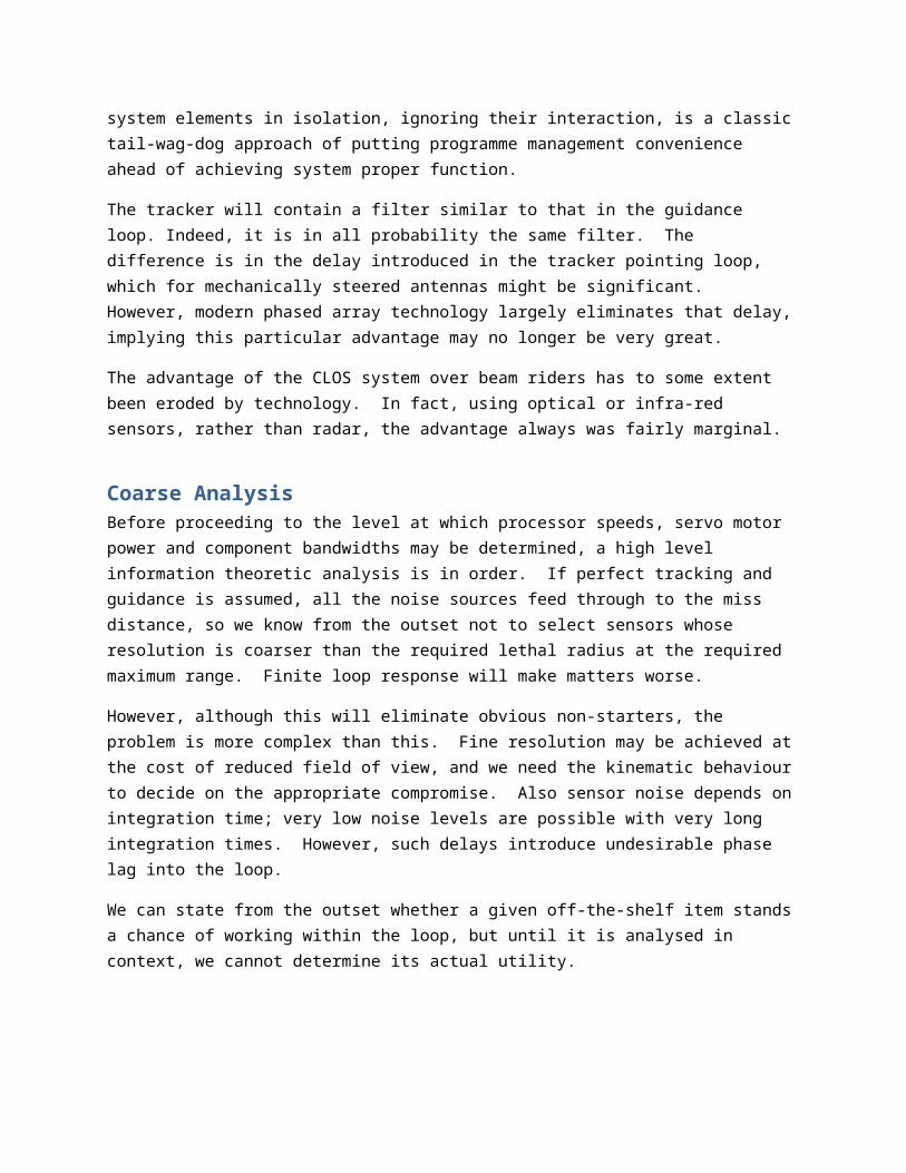
But this is a common trend in systems. Higher performance usually requires tighter integration. The modern tendency to try and treat system elements in isolation, ignoring their interaction, is a classic tail-wag-dog approach of putting programme management convenience ahead of achieving system proper function.

The tracker will contain a filter similar to that in the guidance loop. Indeed, it is in all probability the same filter. The difference is in the delay introduced in the tracker pointing loop, which for mechanically steered antennas might be significant. However, modern phased array technology largely eliminates that delay, implying this particular advantage may no longer be very great.

The advantage of the CLOS system over beam riders has to some extent been eroded by technology. In fact, using optical or infra-red sensors, rather than radar, the advantage always was fairly marginal.

Coarse AnalysisBefore proceeding to the level at which processor speeds, servo motor power and component bandwidths may be determined, a high level information theoretic analysis is in order. If perfect tracking and guidance is assumed, all the noise sources feed through to the miss distance, so we know from the outset not to select sensors whose resolution is coarser than the required lethal radius at the required maximum range. Finite loop response will make matters worse.

However, although this will eliminate obvious non-starters, the problem is more complex than this. Fine resolution may be achieved at the cost of reduced field of view, and we need the kinematic behaviour to decide on the appropriate compromise. Also sensor noise depends on integration time; very low noise levels are possible with very long integration times. However, such delays introduce undesirable phase lag into the loop.

We can state from the outset whether a given off-the-shelf item stands a chance of working within the loop, but until it is analysed in context, we cannot determine its actual utility.

Loop Analysis/DesignThe majority of texts on weapon guidance have a tendency to treat the missile guidance loop in isolation, hence there is a widespread belief that beam rider and CLOS are kinematically equivalent. We hope that the previous section has dispelled that particular myth.

We need to consider both tracker and guidance loop to indicate, in fairly general terms, i.e. what we expect to see in the loop. Any more detailed description is likely to be system-specific and outside the scope of this text.

TrackerRegarding trackers, there is a range of potential options, and a complete discussion of sensor types and their attributes would be a major work in its own right, and would not really be relevant. We are concerned with how the tracker behaviour influences miss distance, without reference to the details of how it actually works. Indeed, we do not want to pre-judge the type of sensor to employ, but need a means of assessing how the sensor parameters affect miss distance.

Strangely enough, modern object-oriented system analysis actually begins with existing elements, as opposed to finding out what they should be from a flow down from proper function. As the latter approach tends to be highly numerate, it is confused by the ignorant with design.

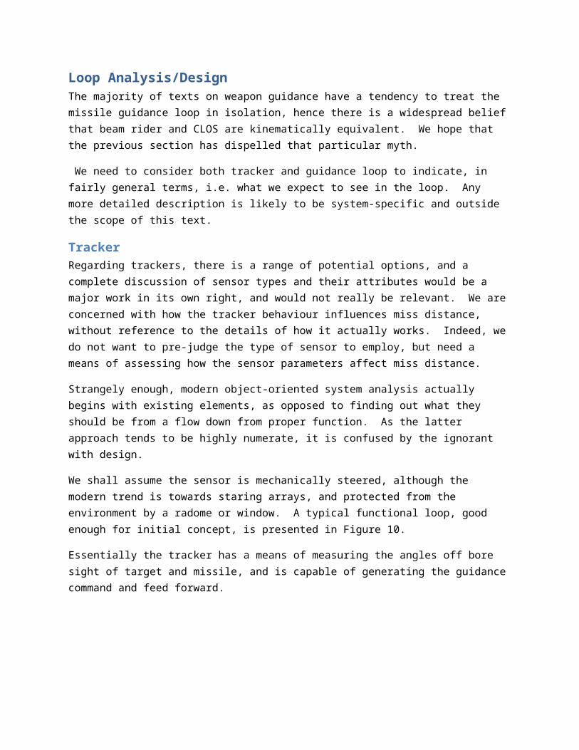
We shall assume the sensor is mechanically steered, although the modern trend is towards staring arrays, and protected from the environment by a radome or window. A typical functional loop, good enough for initial concept, is presented in Figure 10.

Essentially the tracker has a means of measuring the angles off bore sight of target and missile, and is capable of generating the guidance command and feed forward.

Figure 10 : Conceptual Tracker Loop

We have represented a tracking filter as a second order lag, largely so that some representation of its bandwidth is present in the loop. We can determine the sensitivity of the system to this assumption as part of the analysis. If it proves critical, more detail will obviously be needed.

One important point, by representing everything as continuous time functions we are not pre-supposing an analogue implementation. That is a common misconception of the technically naive. The filter is actually expected to be implemented digitally.

However, we begin with the continuous system representation, as this is the ideal. Introducing the z-transform representation, anti-aliasing filter, processor delay and zero order hold, with the introduction of quantisation noise, degrades the ideal behaviour. The issues of implementing the processing digitally are addressed in the analysis.

The guidance error is assumed extracted from an identical tracking filter as is used to track the target, although this need not be the case.

The input to the tracking filter is the bore sight error corrupted by measurement noise. The filtered estimate of bore sight error is fed via a compensator, which dominantly acts as the loop stiffness, which is combined with a rate feedback to generate the input to the torque motor needed to steer the antenna.

There may be some disturbance torques also acting, e.g. structural vibration, and these are included as the disturbance: ‘d’.

Not all tracker options will have all of the elements depicted, so the consequences of their omission in the particular system context need to be assessed. Also, the ingenious designer may think of extra bells and whistles which may be added, but Figure 10 represents an effective starting point for the analysis.

The world of automatic control furnishes us with a cornucopia of methods which allow us to relate behaviour to system parameter values, and hence form the rational basis for a system specification. This is in stark contrast to the pseudo-scientific hocus pocus which has become the current fashion. There are plenty of books on the subject, and courses are offered at universities, for anybody interested in genuine system science.

The tracking filter serves essentially to prevent the (wide band) measurement noise leaking through into the servo, and also into the guidance loop. This implies a low pass characteristic which introduces a de-stabilising phase lag into the loop. This, in turn, may limit the pointing loop bandwidth, potentially introducing greater kinematic tracking error. In the extreme, the target may be lost from the field of view.

Usually, the tracker will require a wide beam for initial gather of the missile on to the bore sight, and loop parameters may be different for this phase of flight. This is important, because gather invariably determines the minimum engagement range and must be done quickly.

There are occasions when, no matter how the loop is tweaked, it cannot be made satisfactory with the values of measurement noise, and measures, such as increasing the signal power, would need to be considered.

Guidance LoopThe actual guidance loop is similar for both beam rider and CLOS. The beam rider believes the guidance beam bore sight is aligned perfectly with the target, except perhaps for a deliberate lead angle. The CLOS system is commanded by differential missile/target error, and is not too concerned where the tracker bore sight is, provided the tracking error is less than the beam width. The target tracking errors lie outside the guidance loop, so the missile sees a guidance error corrupted by tracker noise.

Figure 11 : Typical Guidance Loop Structure

The essential features of the guidance loop are presented in Figure 11. The angular guidance error is converted into a position error using an estimate of the range. This range estimate need not be particularly accurate, as any error amounts to a small variation in loop gain from its intended value. As this is a null-seeking system, it will have no effect on the equilibrium, and only a minor effect on the settling time. A stored value of range versus time is often adequate.

In a radar system, range may be a means of discriminating target from missile, and may well be available.

The phase advance term is part of the compensator, but is presented explicitly because it is fundamental to loop stability. The rate of change of position error must be known to provide damping of the loop, this cannot be measured, so must be estimated. The compensator contains the pole for the phase advance and further phase advance to recover the phase loss in the autopilot.

The phase advance amplifies noise and can cause control saturation, so there is a limit as to how much can be used.

The faster the missile response, the less phase advance is needed, so the noise requirements cannot be known until there is a reasonable estimate of the autopilot bandwidth.

One approach is to generate a population of fly out trajectories of a point moving at constant speed along a line joining the launch point to the target, and taking the Fourier transform of the lateral acceleration histories in order to characterise the set of engagements as a spectrum. The half power width of the spectrum gives an indication of the bandwidth required of the guidance loop, from which the autopilot bandwidth may be derived.

Alternatively, if the missile is ‘given’ we can use the linear-quadratic optimal control result for guidance loop bandwidth:

ωn2=Loop stiffness= ng

xm

Where g is the acceleration due to gravity, n is the lateral acceleration capability in gs and xm the desired miss distance.

Only in university examinations are things ‘given’, and the emphasis is on the solution method. In the real world, it is up to the engineer to find a mathematical formulation which is adequate for his/her purposes. Usually, this is what separates the men from the boys.

Miss DistanceAfter a few iterations we arrive at a few viable tracker/guidance loop options. The transfer function from each noise source to miss distance can be found. The contribution of the ith noise source to miss distance is found from the noise integral:

σ i2= 1

π∫0∞

Gi ( jω ) Gi (− jω ) dω

Where: Gi(s) is the transfer function from the ith noise source to the miss distance, and σ denotes the standard deviation. The miss distance is then found from:

σ m2=∑

1

n

σ i2

This is not the complete picture, as this is the statistical distribution about the point of closest approach, which is not necessarily coincident with the target. Some residual kinematic error is to be expected, particularly near the edges of the coverage diagram.

Strictly speaking, the noise statistics depend on target range, so are unlikely to be stationary processes as is implicit in the white noise assumption on which the noise integral is based. If the statistics don’t change much within the loop settling time, this doesn’t really matter, and consequently it is standard

practice to treat all noise sources as stationary, and to repeat the calculation over the complete ambit of target ranges.

The purpose of this calculation is to identify which noise sources are dominant, so that their effects may be tackled with the highest priority. It is not usually intended as a means of producing definitive performance predictions. The tendency of managers to cite work in progress estimates as absolute and achievable performance predictions, is probably the greatest inhibitor of proper system analysis which is imposed on the modern designer by those whose experience is limited to the design of databases.

Note that none of the calculations needed to characterise the system involve the detailed fly-out model, so beloved by non-participants. Indeed, until the analysis is done, we actually don’t know what to put in the detailed model.

GatherThe two most important phases of flight, are probably the start and the end. What happens as the missile flies past the target is obviously important, so also is the launch and initial gather. The rest of the flight is generally of secondary consideration, yet accounts for most of the run time of a fly out model.

We have considered miss distance analysis, which covers the target end. The principal issue of the launch end is how soon the guidance loop can be closed. It is often impractical to co-locate sensor and launcher. Rocket plumes and radomes do not mix well. Early systems relied on ballistic flight from launcher to beam, which placed a severe constraint on launcher/beam separation. More modern systems may be fitted with a simple inertial navigation system to guide the missile into the gather beam. With low cost solid state sensors and very short IN guidance phases, this is achievable fairly cheaply.

We shall address guidance under inertial navigation in a later section, for the moment we shall consider the line of sight guidance problems specific to the gather phase. Unlike the guidance phase, when the missile speed is roughly constant gather takes place with the missile still accelerating. This introduces a motor thrust term perpendicular to the beam.

Figure 12 : Kinematics During Boost

From Figure 12, we see that in addition to the lateral acceleration fy, there is a thrust term perpendicular to the beam:

f 2=f x (α+γ )

Assuming the beam is stationary, the direction of the velocity vector relative to the beam is given by:

γ=sin−1( yUm )≈ y

Um

The angle of attack may be estimated from the trim condition, which can be shown to be, approximately:

α≈( mY β ) f y

Where m is the missile mass and Yβ is the lateral force per unit angle of attack. This is a stability derivative, which will be discussed when we consider autopilots.

So the lateral acceleration relative to the beam, taking account of the longitudinal acceleration, is:

f 2= f x( mY β ) f y+f x

yUm

Figure 13 : Longitudinal Acceleration Terms

Note if the beam is rotating, the second term becomes:

f x( y−R θ )

Um

Where θ is the slew rate and R is the range.

The effect of these terms on the guidance loop may be derived from Figure 13. We have lumped the phase advance and loop gain into the compensator in order to avoid clutter. Evidently, if the missile is accelerating, the loop gain is increased significantly due to the extra acceleration component attributable to the motor thrust.

What is worse, there is a positive feedback of lateral velocity, providing negative damping to the loop. This is compounded by the fact that the feedback gain is time-varying - effectively feeding a spurious time varying velocity error into the loop. To some extent this may be offset by increasing the amount of phase advance and reducing the loop gain. Usually, however, the loop cannot be closed until the speed has become large compared with the longitudinal acceleration.

It is undesirable to have a rocket motor burning during the guidance phase. The plume obscures the view of both target and missile and attenuates the radar return and command link power. A boost/coast profile is often employed to avoid this potential problem. During the coast phase the longitudinal acceleration is negative, so the loop gain is reduced and the kinematic feedback of lateral velocity is negative, both these effects improve stability but result in a lower loop bandwidth from that calculated by ignoring the deceleration.

General Line FollowingWhen under inertial navigation control the missile position is no longer measured relative to a sensor beam, instead the sight line is a line in space, the position, direction and slew rates of which may be sent

to the missile from the platform sensors at launch. The significant separation between launcher and sensor means the guidance error can no longer be considered small. A more general means of navigation along a line is needed.

The line following geometry is presented in Figure 14. The line segment is defined by its start point vector OA and the vector in the line direction AB.

The position vector of the missile relative to the line start point is:

p=r−aWhere r is the position vector of the missile relative to the origin and a is the vector OA. A single character is used for compatibility with the equation editor.

The projection of this on to the line is:

|b|=p⋅b

Where b is the unit vector in the direction of the line.

Figure 14 : General Line Geometry

It follows that the perpendicular position error relative to the line is:

e=p−|b|b

We cannot assume the missile velocity vector is nearly parallel with the line, as it is when position errors are measured with a guidance beam. So rather than deriving a conventional CLOS acceleration term as a linear combination of position error and its rate of change, we first derive a heading direction from the position error.

Figure 15 : Calculation of Heading

The desired heading direction is based on the requirement for the velocity demand magnitude never to exceed the actual missile speed. If the velocity perpendicular to the beam is proportional to the position error, it follows that the remaining component of velocity must act along the beam. Hence the heading

demand is the unit vector uD calculated from the velocity triangle of Figure 15:

uD=−k y

Ume+√1−( k y|e|

Um )2

b

Where ky is the ‘stiffness’ gain.

When the term in the square root becomes negative, the required missile heading is perpendicular to the line, and it is impossible to approach it any faster.

The required lateral acceleration is now calculated from the difference between the current heading and the desired heading.

The sine of the heading error is found from the cross product of the desired heading direction with the current heading, so the heading hold would aim to set the turn rate proportional to this error:

ωv=k v uD×um

Where kv is the velocity gain.

This rate of turn implies a lateral acceleration given by the cross product of the turn rate with the current velocity vector:

f =U m×ωv

The result is a vector box product:

f =k v Um (um× uD×um )

=k vU m ( uD−(uD⋅um ) um )

Experience has shown that control divas tend to lack the integrity or honesty to admit to not understanding three dimensional geometry, so this algorithm is protected by self importance, which is much more effective than any patent rights.

We calculate the loop gains from the requirement to settle on the beam when it gets there. Evidently when the position error is small the velocity vector is nearly parallel to the line.

This situation is presented in Figure 16.

Figure 16 : Small Errors

The component of velocity in the direction of the line is very nearly equal to the missile speed, so we need only consider the perpendicular component. The heading error demand becomes:

γ D=−k yy

Um

We note that:

uD⋅um=cos (γD−γ )≈1

So the acceleration equation becomes:

f y=k v Um (γD−γ )=−kv k y y−kv U mγ=−kv km y−kv y

The control scheme reduces to a second order system whose gains are easily calculated.

Thrust Vector ControlThe line-following algorithm presented in the previous section using aerodynamic lift to generate lateral acceleration, is probably suitable for mid-course guidance between way points under inertial navigation/GPS sensors. However, during launch, the speed is initially too small for the aerodynamic forces to be effective. The only significant force available is the motor thrust.

In fact, the low speed implies lower centripetal force is needed to steer the missile on to the desired heading. In order to achieve a reasonable minimum engagement range, it is therefore more advisable to exploit the motor thrust to turn the trajectory quickly at the very start of flight, than it is to defer manoeuvre until the speed has built up sufficiently for aerodynamic control to become effective.

By deflecting the thrust perpendicular to the body, or by using ‘bonker’ motors to apply impulsive moments the orientation of the missile body, and hence the direction of thrust in space can be controlled.

The orientation of the missile may be defined as a 3×3 matrix whose columns are the unit vectors along the body x, y and z axes respectively.

T=( x y z )

In this form it is used to transform vectors from body axes to fixed. To transform back, the transform is

used. The aim of the attitude controller is to point the body x-axis in a desired direction in space; xD . The attitude error is given by the cross product of the desired orientation with the current orientation:

ε= xD× x

Resolving this into body axes:

ε B=T T ε=( x⋅ε ) x+ ( y⋅ε ) y+( z⋅ε ) z

Evaluating the three scalar triple products, we have:

x⋅ε= x⋅( x D× x )= xD⋅( x× x )=0y⋅ε= y⋅( xD× x )= x D⋅( x× y )= xD⋅zz⋅ε= z⋅( x D× x )= xD⋅( x× z )=− xD⋅y

The transformation matrix T is central to any inertial navigation system, so will be present. How it is obtained is a matter of implementation.

In essence, we have derived signals equal to the sine of the attitude error expressed in body axes. The attitude control is expected to consist of thrust deflection proportional to this term together with a term proportional to the corresponding angular velocity.

The issue remains as to how we calculate the attitude demand from the desired lateral acceleration.

The problem is identical to that of generating a beam error demand which must respect the finite missile velocity. In this case we are generating an acceleration demand which must take account of the available thrust. The solution is identical.

Our navigation law generates a lateral acceleration vector f. The available acceleration is:

f T=Tm

Where T is the motor thrust, and m is the missile mass. In fact, this term could probably be measured with a longitudinal accelerometer.

By analogy with the line following algorithm, the attitude demand for input to the attitude control loop becomes:

f T x=f +√ f T2−|f|2 um

In this case, when the square root becomes zero, there is no component of thrust acting along the trajectory, and the missile is actually flying sideways. This represents the maximum possible lateral acceleration under thrust alone.

Considering the boost phase only lasts a few seconds, the inertial reference unit does not appear to require a stringent specification. Rapid response time is to be valued over the usual criteria of drift and biases, which are needed for longer duration flights. The instruments which are optimised for conventional inertial navigation systems may not be optimum in this application, and the delay implicit in introducing filtering and synchronisation with GPS probably cannot be afforded in such a short flight.

As is often the case, the optimum in one application is not necessarily universally the best choice. The turnover autopilot of a vertically launched missile will have quite different requirements from a mid- course cruise application.

Concluding CommentLine of sight guidance is often viewed as the poor man’s homing, yet effective systems are still possible using it, and for short range applications is worth considering at least during the concept phase. Some extremely effective line of sight systems have been fielded and proven under actual combat conditions, so it is probably premature to toll its death knell just yet.

Homing Guidance

IntroductionPlacing the main sensor on the missile introduces a degree of autonomy which makes ‘fire and forget’ operation possible. Also, the number of targets which may be engaged simultaneously need not be restricted to the limited number of sensors on the launch platform, nor is there such a severe constraint on platform manoeuvre as would be expected from a line of sight system.

The degree to which these advantages are realised depends on how the system is implemented. In general, we don’t get something for nothing and we can expect a fully autonomous fire and forget missile to raise its own issues, such as aborting the engagement when targets are incorrectly identified (e.g. friendly fire). Apart from fairly short range systems, where positive target identification is possible before launch, we should expect the missile to be supported by additional sensors on the launch platform. The level of actual autonomy appropriate depends on the nature of the threat, the launch platform constraints and the operating environment.

Generic Sensor TypesThe design and selection of sensors is a major topic in its own right, and we would be deviating from our system level presentation if we presented more than a rather sketchy introduction.

As mentioned elsewhere the classification of sensors reflects their influence on the overall system (the degree of potential autonomy). The three principal categories are:

Passive Semi-active (or bi-static) Active

PassiveA passive sensor detects the energy (of whatever form) emitted by the target. This may be radar or communications emissions, infra red, visible light or ultra violet. In a sense visible light band emissions are dominated by reflections from the Sun or other light source rather than actual passive radiation.

Anti-radiation seekers are a subject of on-going classified research, and will not be discussed further.

Early infra-red detectors were fairly insensitive and could only detect the hot jet pipe of the target, against a clear sky background, so could only be used for air to air or surface to air engagements. The atmosphere is fairly opaque to infra-red except in the 3 to 5 micron and 8 to 13micron wavelength windows. The 8 to 13 band is known as the ‘thermal band’, because it corresponds to the black body

radiation peak at ambient temperature, so that the energy available in this band is relatively high. This makes possible the use of an uncooled sensor.

Early seekers used a spinning reticle in front of a single sensing element to detect the target bore sight error, hence modulating the heat source provided a simple means of jamming. Various scanning arrangements have also been used such as line scan and rosette scan to improve the resistance to jamming whilst still using a single element or line of elements. Since the development of charge coupled devices in the 1990s, modern sensors universally have become imaging arrays of elements.

An imaging sensor is not restricted to contrast against a sky background, but can employ pattern recognition techniques to distinguish the target from the background, which is radiating a similar amount of energy. Indeed, it is the contrast of the target with its background which is the principal problem, particularly in land clutter. Sea clutter is not such a problem, except at shallow dive angles, as there is usually ample temperature difference between the sea and a ship target.

Since contrast is what is usually required in an imaging sensor, the thermal waveband loses some of its appeal. Also low cost IR sensors typically employ a micro-bolometer array, which has a significant integration time. This may not matter for reconnaissance missions but imposes severe performance constraints on a guidance loop. On the other hand higher performance arrays, having short integration times usually require the sensor to be cooled, which adds complexity. Bearing in mind the optics associated with IR involve such exotic materials as sapphire and germanium and must be much larger for the longer wavelength than for the shorter, the 3-5 micron band using a cooled sensor becomes more attractive.

The choice is highly application specific, so will not be discussed further, except to say the current practice of trying to down-select seekers on the basis of power point, hand-waving and UML will get us nowhere.

With the Sun to illuminate the scene, there is usually plenty of signal power in the visible band. Modern CCD cameras will actually still work even in starlight, so except for the most overcast dark nights, we should expect a visible band sensor to work. They are inexpensive, since there is an extensive mass market, and the optics use ordinary glass, which is opaque to infra-red. On the down side operating in the 0.4 to 0.8 micron waveband renders the sensor vulnerable to obscurants (smoke), mist, fog and rain. The short wavelength implies the optics can be quite compact compared with infra-red sensors, and could be used as part of a more sophisticated multi-band seeker. Since identification markings are usually only visible in this waveband, a visible band sensor provides a means of positive target identification, which could be relayed back to the launch platform to abort the attack.

Up until the development of focal plane arrays, the only sensor which could be used to discriminate the target from the background in a land scenario was the human eyeball, so anti-tank systems tended to be line of sight or semi-active. Television guided weapons, like the old Martel missile, relayed the image back to the human operator, a form of guidance which would still be effective, but as far as the degree of autonomy is concerned, is probably better classified as a semi-active system.

Ultra violet is usually associated with detecting targets in arctic conditions, where IR signal level and contrast is poor, and white-painted targets are difficult to see in the visible band.

Semi-ActiveThe optical type of sensor is restricted by the low level of target emissions, atmospheric turbulence, attenuation and precipitation to fairly short ranges, so would be restricted to the terminal stage of flight. This opens up the can of worms called target acquisition, which we shall not discuss.

Early missiles were universally ‘lock before launch’, where the correct target acquisition was the responsibility of the launch platform. Longer range passive and active systems are expected to have an autonomous mid course phase before turning the seeker on. This, not surprisingly, is often referred to as ‘lock after launch’.

In a semi-active system, the target is illuminated from a separate source, which may or may not be the launch platform. In the air-to surface case it almost certainly will not be the launch platform which illuminates (paints) the target. A special forces operative on the ground near the target may use a laser designator which fires a coded pulse, or a separate aircraft may illuminate the target at a safe stand -off. Unless one has a death-wish it is not advisable to emit radiation, which can be detected, when operating deep within enemy airspace.

Semi-active radar air-to air systems have been deployed, using a steerable antenna, which yields some launch platform freedom to manoeuvre, but the trend is to active homing, ‘fire and forget’, allowing the launch platform to remain relatively covert.

Semi active has a number of advantages, firstly when used against surface targets, it can use human pattern recognition to identify the target, and invariably the launch platform is capable of generating considerably more power than is available in passive or active systems. The seeker is significantly cheaper than is required for an active system, and the launch platform may provide additional kinematic information on the current engagement conditions.

The need to illuminate the target throughout the engagement restricts the number of missiles which can be kept in the air simultaneously, and exposes the launch platform to the risk of attack by anti-radiation missiles.

These disadvantages may be overcome by only illuminating the target in the end game, with mid-course command guidance. The defence would be scheduled so that the illuminator is switched from target to target whilst each missile approaches its own end game. In this way it is possible to have something like four missiles in the air for each illuminator.

The platform vulnerability issues have tended to dominate current thinking, so that semi-active systems are probably on their way out.

ActiveActive homing guidance requires the illumination energy source to be carried on board, which severely restricts the power available, typically requiring a separate mid course phase to bring the missile close enough to the target for successful acquisition. The seeker is generally very expensive. The limitation to short range keeps the most of the flight covert, giving the target minimal warning of the missile’s presence. The launch platform need not emit radiation, and hence can remain relatively covert, although presumably there must be some means of initial target detection and tracking before the missile can be launched.

Kinematic LimitationsProportional navigation does not impose such severe kinematic requirements on the missile as line of sight guided missiles, and it is fair to say that most of the system limitations arise from the sensor limitations. Range is limited by sensitivity and target signature in the waveband and aspect of interest, although long integration times can improve detection, the extra delay influences guidance loop bandwidth. Increased sensitivity may involve narrow field of view, which may put excessive bandwidth requirements on the sensor pointing loop, or reduce the maximum sight line spin which can be tolerated. The width of the field of view usually also determines the sensor resolution. In addition to the instantaneous field of view, the sensor is typically mounted in a gimbal to decouple it from the body motion. The mounting has limits of travel which limit the maximum look angle (or ‘angle of regard’ according to the terminally pretentious) which imposes a kinematic constraint on the engagement geometry.

Radar sensors, if using continuous wave (CW) modulation, would use Doppler as the target discriminant, and would lose the target in clutter when engaging side-on. Also semi-active systems require a rear phase reference to determine the missiles own Doppler with respect to surface clutter. This implies a body to beam limitation, which may limit the angular separation between the illuminator and the launch point.

Pursuit could impose limitations, if it were used. However, if used in the end game, the missile would first be command guided into the enemy tail aspect, otherwise it might be used, under inertial/command guidance, to reduce the look angle to within the ambit of the gimbal limits before switching to proportional navigation in the end game.

When considering kinematic limitations, the sight line spin limit and look angle limit are probably the most important.

Homing SAM systems can be characterised by forward range/crossing range in the same way as line of sight systems, but more generally, the launch platform motion has a significant effect on the engagement, so it is more informative to consider the air to air case.

The engagement is depicted in its simplest form as a constant velocity target as the same altitude as the attacker (see Figure 17). Early missiles tended to be lock before launch, so the missile was launched

along the sight line from launch platform to target. This constraint need not necessarily apply to modern missiles.

The angle between this sight line and the target velocity vector is called the aspect angle, conventionally it is measured with respect to head-on, it is measured in the plane of the engagement (known as the fly plane).

Figure 17 : Basic Co-Altitude Engagement

The elevation angle of the sight line for the more general case of the attacker and target at different altitudes is known as the ‘snap’ angle. Missile performance is a function of altitude and engagement geometry, so the aircraft is fitted with a sophisticated fire control which provides cues to the pilot as to when the target is feasible.

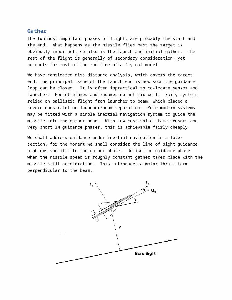
Figure 18 : Ideal Collision Course

Engaging at an aspect angle α, the missile will settle down near a collision course as shown in Figure 18, in which R is the initial range, Um the missile speed, UT the target speed and tgo the time to intercept. The look angle, λ is given by:

sin λ=UT

U msin α

This is a maximum with side-on engagements. Note that if the missile is expected to catch the target in a tail chase it must obviously fly faster. A speed advantage of 2:1 implies a look angle of 30˚should be adequate.

With a steerable dish antenna, the larger the look angle, the smaller the antenna aperture, so increased look angle implies inferior angular resolution, so there is clearly a trade-off. A staring phased array fixed with respect to the body suffers from broadening of the beam and grating lobes when steered to large angles. Optical sensors in all wavebands tend to require much smaller apertures and can be steered to large look angles.

If the target has the speed advantage over the missile, it can only be engaged close to head-on.

As far as sight line spin is concerned, we note that proportional navigation tends to reduce it, so that the maximum value is expected at launch, and the seeker would fail to acquire the target.

The initial sight line spin rate for launch along the line of sight is given by:

ω0=UT sin α

R

This is likely to limit minimum engagement range.

Analysis

ObjectivesWith line of sight guidance we found that the rms miss distance can be calculated from the noise sources using the well-known noise integral. However a homing system is characterised by having time varying coefficients. When deriving guidance laws, it was convenient to express the problem in terms of time to go. However, this is useless for performance analysis, because it yields either infinite or zero miss distance. This is fine for deriving ideal navigation algorithms, and indicating suitable values for the parameters, but completely useless for finding the miss distance of any specific system.

We want a means of finding out how system noise feeds through to miss distance which applies to the time-varying case.

The actual guidance loop is made up of both constant coefficient and time varying elements. Indeed, the missile lags largely account for the kinematic miss distance. This is the reason why discussing values of navigation constant without reference to the missile response is so much nonsense. It is only the inherent robustness of proportional navigation which renders it insensitive to small changes in navigation constant, so that such discussion is, in any case, irrelevant.

In order to illustrate the effect of missile lag, we consider the extreme case of a pure delay. This is mathematically the simplest case to deal with. As our interest is in homing, and not in exotic mathematical methods for their own sake, this seems a wholly appropriate line of enquiry.

We recall the equation for Proportional navigation homing was derived from the zero effort miss distance:

dxm

dt+ N

(T−t )xm=0

Where xm is the zero effort miss, T the initial time to go, N the navigation constant and t the elapsed time.

The solution is:

xm=(T−tT )

Nxm0

A pure delay; τ implies that the actual miss distance corresponds to the value at τ seconds to go:

xm=( τT )

Nxm0

This is now a function of the initial time to go. Differentiating this with respect to T:

dxm

dT=−N 1

τ ( τT )

N+1=− N

Txm

We now have an expression for miss distance as a function of the duration of the fly out:

dxm

dT+ N

Txm=0

This is the same as our forwards time miss distance equation. Curious.

The Adjoint EquationA moment’s reflection reveals that we aren’t interested in the single result for a single fly out, as might be expected from simulating the system in forward time. What we actually want is the miss distance as a function of flight duration, which yields far more insight into system behaviour.

The system is assumed to be time varying governed by a linear, homogenous equation:

x=A (t ) x

Where x is the vector of n system states, which in general, will contain many more elements than the single state of our example.

Supposing we have been through the exercise of simulating the system forwards in time covering the ambit of flight times of interest, we will have generated an array of solutions:

x ( ti )=Φ (0 , ti ) x (0 )

Or, more generally:

x ( t1 )=Φ ( t 2 ,t1) x (t 2)

Where Φ is the array of solutions, each element of which is an n×n matrix. This could conceptually be generated by applying an impulse at each start value and summing the effect on each end value, and repeating the process for every start time and every state.

As the interval between successive solutions becomes infinitesimal, and the number of elements becomes infinite, we talk of a transition matrix. We can think of this as the ‘brute force and ignorance’ approach, which is all too common.

x ( t2 )=Φ (t 1 ,t2) x (t 1)=Φ (t 1 , t2 )Φ (t2 , t1) x (t2)

From which:

Φ ( t1 , t 2)Φ (t 2 , t1 )=I

Figure 19 : Illustration of Transition Matrix

The time samples at which the solutions are stored are effectively the indices of the array Φ, so the reverse order of the indices is exactly the same as the transpose of the transition matrix. So we may write:

Φ−1=ΦT

In other words, the inverse of a transition matrix is its transpose.

We want to specify the end state (i.e. apply an impulse at the final miss distance) and find out its sensitivity to each of the inputs, as functions of time to go.

The final state is related to the state at a specified time to go by:

x (T )=Φ (T−t , T ) x (T−t )

The state at the time to go which would result in the end state is:

x (T−t )=ΦT (T−t , T ) x (T )

Writing in terms of time to go; tgo=(T-t):

x ( tgo )=ΦT (t go ,0 ) x (0 )

The problem reduces to finding the equation governing x(T-t).

The forward time equation is known, and yields the solution:

x (t )=Φ (0 ,t ) x (0 )

Where x(0) is the state at the start of the interval of times to go of interest, i.e. the start of the single fly out of duration T.

Differentiating:

dxdt

=dΦ (0 , t )

dtx (0 )=A (t ) x

It follows that:

dΦ (0 , t )dt

=A (t ) Φ (0 , t )

The end state is given by

x (T )=Φ (t , T ) Φ (0 , t ) x (0 )

Or: x (0 )=ΦT (0 ,t )ΦT (t , T ) x (T ) )

Differentiating:

dΦT (0 , t )dt

ΦT ( t ,T )+ΦT (0 , t ) dΦT (t ,T )dt

=0

ΦT (0 , t ) AT ( t )ΦT (t , T )+ΦT (0 ,t ) dΦT (t , T )dt

=0

We should not expect the transition matrix to be singular, so:

dΦT ( t ,T )dt

=−AT ( t )ΦT ( t ,T )

Now for the sample at time t, an increment in forward time is the same as an equal decrement in time to go, so:

dΦT (t ,T )dtgo

=AT ( t )ΦT (t , T )

The time sample t is precisely the same as the sample T-t in the final column of the transition matrix shown in Figure 19, so we are justified in writing:

dΦT ( tgo ,0)dtgo

=AT (t go )ΦT ( t go ,0 )

By implication:

x ( t go )=AT (tgo ) x (T )

The state expressed in terms of time to go is usually called the ‘adjoint’ state to distinguish it from the forward time state. It may be considered the sensitivity of the end state to the forward time state expressed as a function of time to go. The equation above is known as the adjoint equation, and forms the basis of a powerful method of analysis of homing guidance systems.

We now see why the single state example with the missile lag represented as a pure delay yields an adjoint equation which is identical to the orginal system equation the system ‘matrix’ is a scalar which is obviously equal to its own transpose.

Adjoint MethodWhilst the modern trend is to brute force and ignorance, generally imposed by those who seem suspicious of powerful mathematical techniques, we shall unrepentantly continue to follow the path of wisdom.

Analytical solutions of terminal controller problems are rare, and the important ones may be found in the textbooks. When we start mixing time-varying coefficients and constant coefficients, we invariably must resort to the computer. The adjoint method indicates that the best approach is not the over-priced computer game, but techniques which yield the maximum insight for the minimum investment of effort.

As a simple illustration, consider representing the missile response as a first order lag:

f y=1τ (NU c ω−f y )

ω=f y

U c (T−t )−2

(T−t )ω

Where τ is the missile lag.

Or in matrix form:

( f y

ω )=( −1τ

NU c

τ1

U c (T−t )− 2

(T−t ) )( f y

ω )

Figure 20 : Comparison of Forward Loop and Adjoint Loop

The adjoint equation is:

( y f

yω)=( −1

τ1

U c t go

NU c

τ− 2

tgo)( y f

yω)

The notation y with the subscript of the corresponding forward state is used to indicate that it is a sensitivity of the end state to the forward time state.

We usually draw out the control loop so that the cause/effect relationships and information flows are easier to identify than is possible with the modern practice of lumping everything into a single matrix. The construction of the adjoint loop from the forward loop is particularly easy. The main rules are:

Make sure all comparators are converted into summing junctions by including gains of value -1, as appropriate

Replace all summing junctions with simple connectors and simple connectors with summing junctions

Reverse all signal flow directions so that inputs become outputs and vice versa. Inputs are usually step functions rather than impulses so an extra integrator

may be needed in the adjoint loop.

These rules have been applied to the missile lag + sight line kinematics system, resulting in Figure 20.

Crude Seeker ModelMuch of the complexity of the guidance is to be found in the seeker processing, so we shall restrict ourselves to a simple representation.

The seeker sensor is often mounted in a gimbal to isolate it from the missile body motion, although there is a trend towards body fixed staring arrays. This measures the direction of the target relative to the bore sight, and steers the gimbal to cancel the boresight error.

Consider a pointing loop in which the torque applied to the gimbal is proportional to the boresight error and the boresight angular velocity. The bore sight error is::

ε=φT−φ

Where φT is the target sight line direction and φ is the bore sight direction with respect to inertial axes.

The equation of motion is:

I φ=−T ε ε−T v φ

Where I is the moment of inertia and, the Tx are the torques proportional to state x.

The pointing loop is presented in transfer function form in Figure 21.

Figure 21 : Simple Pointing Loop

The transfer function relating the input target sight line direction to the boresight error may be found:

ε ( s )=φT ( s)−ε (s ) 1s ( K ε

s+K v)

i.e:

εφT

=s (s+Kv )

s2+K v s+K ε

=G (s )

The final value theorem yields the result that the long term bore sight error is the value of:

ε=sG ( s )φT ( s )

As; s→0.

If the sightline is fixed:

φT ( s )=φT

s

For which the steady state bore sight error is zero. However, a constant sight line spin, φT = ωt, has the Laplace transform:

φT ( s )=ωs2

This yields the steady state boresight error:

ε →ωK v

K ε

i.e. the bore sight error is an estimator of the sight line spin rate.

If the gimbal rate is measured with, say, a gyro, there will be an inevitable bias on the rate estimate. This is denoted δ in Figure 21. The transfer function from gyro bias to bore sight error is:

εδ=

s+K v

s2+K v s+K ε

Applying the final value theorem to this shows that the steady state bias on bore sight error becomes:

ε bias=δK v

K ε

In order to minimise the effect of gyro bias, the bandwidth of the pointing loop must be as high as possible. There will be restrictions on the available servo motor power, and noise in the loop from the sensor, making high bandwidth only achievable at considerable cost. Modern low cost solid state gyros may look attractive, but the extra bandwidth required to suppress the bias may involve considerably greater expense than was saved with the cheaper components.

Early infra-red homing missiles mounted the sensor in a spinning gyroscope, and used the currents needed to drive the torque motors as estimates of the sensor angular velocity. This approach was synergetic with the spinning reticle needed to estimate target direction.

High loop gain is needed for high seeker bandwidth and suppression of biases, whilst low gain is needed to suppress noise. The compromise adopted depends on the specific target set and engagement conditions, for the missile in question. We should expect the gains to be functions of time to go, as the measurement noise is expected to reduce as the range reduces, and higher seeker bandwidth is needed to accommodate the higher effective bandwidth of the sight line kinematics.

It is evident that designing a seeker for proportional navigation, which will fit in the limited space available is no mean feat, and seekers are usually very expensive items as a consequence. Pursuit just requires the measurement of the boresight error, with perhaps some means of estimating the body orientation with respect to the velocity vector, and is far less demanding.

Representative Homing Loops

Figure 22 : Homing Loop KInematics

The analysis of the loop begins with the description of the sight line kinematics which is presented in Figure 22. We shall consider pursuit, PN using the seeker kinematics derived in the previous section and PN using a more sophisticated seeker.

Sight Line Kinematics

Figure 23 : Sight line Kinematics Forward Model

The zero effort miss distance is given by:

xm=( yT− ym )+(T−t ) ( yT− y m)

Also:

yT− ym= f T− f y

These equations are represented in transfer function form in Figure 23, we have taken miss distance as the output.

The adjoint model of the sightline kinematics follows the rules already presented (see Figure 24). However, an extra integrator is introduced into the lateral velocity node. This is because the actual input to the forward model is a step function and not an impulse. This integrator should really have been present in the forward loop, but in practice it is more convenient to deal with a step function than an impulse when simulating the system numerically.

This output from the adjoint model is the sensitivity of the end state to initial aiming error, i.e. the deviation of the initial velocity from the aim direction. It has been converted to an angle in radians by dividing by the missile speed.

Note that there is no equivalent sensitivity output corresponding to the position offset. This is because the adjoint system generates the relationship between start state and end state, and avoids all the usual intermediate time steps. All runs begin on the axis, because our aim direction axis is defined as the line from launch point to the target at the start of the simulation. It is therefore nonsense to imagine any

initial lateral displacement at the beginning of flight. This is simply an intermediate adjoint state which has no useful interpretation in the forward simulation.

Figure 24 : Adjoint of Sight line Kinematics

All the mysticism of adjoint simulation disappears when we have a clear understanding of precisely what the results mean. We are not ‘running time backwards’. Adjoint time is the time of flight. We are producing the sensitivities of end state to start state for an ambit of times of flight, and doing so in a single run, rather than running the forward model thousands of times.

Since the miss distance input to the adjoint model is an impulse, the feed forward gain (T-t) to the lateral velocity state is redundant, as it is zero when the impulse is present, so this may be safely omitted.

PursuitIf used at all, pursuit would engage the target from the rear, having manoeuvred into the tail region under inertial/command guidance. Range at acquisition is expected to be short, so the seeker signal processing is not expected to introduce significant delays, and the sensor is expected to be body mounted so there are no gimbal dynamics to concern us.

We assume the sight line can be resolved into velocity axes. There are many ways of achieving this, for example mounting the sensor in an aerodynamically stable forebody, or using angle of attack vanes.

The missile will take a finite time to respond, so it appears the only the autopilot lag need be included, to begin with, at least.

Figure 25 : Pursuit - Forward Model

The pursuit loop is presented in Figure 25. It is in principle very simple, but pays the penalty of limited coverage. However, it is possible that by putting some intelligence into the remainder of the system ( i.e. command guiding on to a tail chase), such low cost weapons could be exploited effectively.

Figure 26 : Pursuit Adjoint Loop

Constant coefficient transfer functions are self-adjoint, so there is no need to re-arrange the signal flows within the autopilot lag.

Note that we have also taken the lateral acceleration as an output. This is because we expect pursuit to fail as a consequence of control saturation rather than miss distance. The adjoint system will therefore be run both for miss distance and terminal latax. In order to proceed we need some representative values of system parameters.

The target is expected to have a finite response time so we have included a first order lag to represent this.

We shall arbitrarily select the missile speed as 600ms-1, as we should expect it to have some speed advantage over potential targets. An autopilot bandwidth of 10Hz doesn’t seem too ambitious and a Butterworth pole pattern appears appropriate We know that the pursuit gain must be high, so say 10000.0 ms-2/radian (1g per milliradian), to ensure the velocity vector points at the target at all times. The target is presumably much larger than the missile, so we shall assume a time constant of 0.1 seconds.

The closing speed is one of the parameters we wish to investigate explicitly. At this stage we wish to investigate the validity of the control saturation criterion:

Um

U c>2

We shall consider a 350ms-1 target in head-on and tail chase, corresponding to closing speeds of 950ms -1 and 250ms-1 respectively.

About ImpulsesA further point is the representation of the impulse needed as the input to the adjoint model. Impulses are, like weightless blocks, inextensible strings and frictionless pulleys, mathematical fictions which make the sums less cumbersome. They have no actual existence, so that when we come to model them, we need to know how close an approximation to the ideal is ‘good enough’ for our purposes. The best we can do is a rectangular pulse having duration equal to a single time step.

Evidently, what constitutes ‘instantaneous’ depends on the time interval which is of current interest. In the absence of better information, time intervals of 100th this value are instantaneous, and anything which is 100 times this value is constant. Quite often we can get a fair idea of what is going on when the multiplication factor is reduced to 10.

As the sage put it; it is better to use an approximation and know the truth within a few percent, than to insist on an exact answer and know nothing about the truth. Most numerical work is concerned, not with getting the answer, but deciding on how accurately the answer is calculated.

Provided the triangular pulse has the same effect as a true impulse, there should be no problem. As it is the spectral content of the signal which concerns us, our best bet is to examine it in the frequency domain. The Laplace transform of a true impulse is unity. For a rectangular pulse it is:

I ( s )=∫0

T

e−sT dt=[−e− sT

s+ 1

s ]=1−e−sT

s

The model dynamics is not concerned with frequencies above, say ωm, which we take as the upper bound on s:

I (ωm )=T−ωnT 2

2!+…

This is near enough a true impulse if:

ωmT <2δ

Where δ is the allowable error in the impulse. However, the simulation time step is typically selected on the basis of one tenth the shortest characteristic time constant of the system, which is a more stringent requirement than maintaining the fidelity of the impulse. So for the level of detail and accuracy expected from a linear analysis, we are justified in using a rectangular pulse equal in duration to the time step and having amplitude equal to the reciprocal of the time step.

In order to avoid modelling impulses altogether, it is easier to assign the state variable of the integrators having the adjoint miss distance as input to unity.

Pursuit ResultsConsidering first the head-on case, the miss distance results are misleading. The sensitivity to initial aiming error is practically zero.

Figure 27 : Head-On Case - Miss due to Aiming Error

At first sight, pursuit appears to achieve a direct hit regardless of the aiming error.

Figure 28 ; Head on Case - Miss Distance due to Target Manoeuvre

The target manoeuvre sensitivity is not so encouraging, as it appears to indicate that a mere 1g will cause about 45m miss distance.

Figure 29 : Final Latax Sensitivity to Aiming Error

The aiming error also has very little effect on the terminal lateral acceleration.

Figure 30: Head On Engagement Final Latax Sensitivity to Target Acceleration

As can be seen from Figure 30, target acceleration has a catastrophic effect on the terminal lateral acceleration, requiring of the order of 100 times the target manoeuvre capability.

Quite apart from the glaringly obvious effect of target manoeuvre, all these plots have the undesirable feature that the end state worsens the longer the fly-out. This implies that the guidance error builds up during the flight and is only corrected near the end. The longer the period before the guidance becomes effective, the greater the built-up guidance error. This is not a satisfactory behaviour.

Figure 31 : Tail Chase Miss Distance Sensitivity to Aiming Error

For the tail chase, the absolute values of miss distance sensitivity are much smaller than for the head-on case. More importantly, it reduces with increased time to go, implying the majority of the course correction occurs early in the flight. This is a much more satisfactory behaviour.

Figure 32 : Tail Chase Miss Distance Sensitivity to Target Acceleration

The target acceleration sensitivity in the tail chase is much reduced; the target would need to pull 100g to increase the miss distance to 4m or greater.

0 2 4 6 8 10 12

-0.012

-0.01

-0.008

-0.006

-0.004

-0.002

0

0.002

0.004

Tail Chase Latax Sensitivity

Time to Go (sec)

Lata

x pe

r Rad

ian

(m/s

/s)

Figure 33 : Tail Chase Final Latax Sensitivity to Aiming Error

In the tail chase the lateral acceleration sensitivity plots are similar to the miss distance sensitivity plots, because, as we have seen, control saturation does not occur under these circumstances, as is commonly, and erroneously, believed.

0 2 4 6 8 10 12

-0.3-0.2-0.1

00.10.20.30.40.50.60.7

Tail Chase Latax Sensitivity

Time to Go (sec)

Lata

x pe

r m/s

/s (

m/s

/s)

Figure 34 : Tail Chase - Sensitivity of Final Lateral Acceleration to Target Manoeuvre

We note that the peak terminal lateral acceleration is 0.6 that of the target in the tail chase. The target actually needs greater manoeuvre capability than the missile in order to escape.

Mark Twain once wrote that it wasn’t what people don’t know that makes them stupid, it’s what they do know that ain’t so. These results illustrate the closing speed condition for pursuit guidance to work, which was discovered during the initial analysis Indeed, when operated within its feasible region it exhibits considerable robustness to target manoeuvre. This might in part explain why in predator/prey encounters in Nature, millions of years of evolution has settled on pursuit as the navigation law of choice.

Proportional NavigationProportional navigation systems have been analysed competently elsewhere. We shall restrict ourselves to a basic loop, with target acceleration, aiming error and the sensor angular measurement noise. In fact, there are additional noise sources such as the gyro bias on the seeker angular velocity measurement.

Guidance loop bandwidth is often limited by the parasitic loop due to radome aberration. This introduces an error on the bore sight angle measurement, which depends on the orientation of the body with respect to the sight line. These effects would need to be considered in the specific system under consideration.

More modern systems would include more sophisticated sight line filtering, than is implicit in the seeker model used here, but to avoid the risk of divulging proprietary information, this will not be discussed.

The seeker model uses bore sight error as the estimate of sight line spin, effectively differentiating a noisy sensor measurement.

Figure 35 : Basic Proportional Navigation Loop

In order to prevent the noise from reaching the autopilot servos it is common practice to include a low pass filter between the seeker measurements and autopilot input. This is known as the inter-loop coupling filter. More sophisticated seeker processing ought to render this filter redundant.

Figure 36 : PN Adjoint Loop

Using The Adjoint ResultsProportional navigation has been thoroughly investigated elsewhere; it is by far the commonest navigation law in use. However, our objective is to introduce ideas which are not widely known, so we shall concentrate on how the adjoint simulation results may be used in noise studies.

The adjoint solution is an impulse response (h(t)) of the final state to the input at the time to go. We can therefore find the effect of the miss distance due to an input y(t):

x (T )= 1T ∫

0

T

h ( t ) y (t ) dt

Assuming the noise source is uncorrelated we have, for the variance of the end state:

σ x2 (T )= 1

T ∫0

T

h2 ( t )σ y2 (t ) dt

The adjoint solution furnishes the means of identifying the effect of each of the noise sources on the end state, enabling the most critical disturbances, and the time at which they have greatest effect, to be found.

Estimation of Sight Line Angular VelocityHowever the sight line spin is estimated, it must be with respect to inertial axes. There are many ways of achieving this. Most methods require the sensor to be mounted in a gimbal, so that it is space stabilised. This not only ensures that measurement is with respect to inertial axes, but also isolates the sensor from the missile body motion (except for radome aberration effects). This places restrictions on the sensor aperture, and is also very expensive. We have seen how a high bandwidth pointing loop can serve to reduce the effect of gyro bias on sight line spin estimation. However, the cost and limitations of the practical seeker has motivated considerable research into so-called ‘strap-down’ homing guidance.

By ‘strap-down’ we mean the sensor is rigidly mounted on the body of the missile, as in pursuit guidance. This requires an accurate measurement of the body angular velocity, implying a much higher quality sensor than would otherwise be required. Much effort has been applied to estimating the gyro bias, but fundamentally the problem is akin to trying to lift oneself into the air by pulling on one’s own boot laces.

One approach to reducing bias is to use an observer based on the sight line kinematics to improve the quality of sight line spin estimate.

We know that the sight line spin is expected to vary with time according to:

ω=2ωt go

−f y

U c t go

This takes feedback from the lateral acceleration (usually required for the autopilot and/or inertial measurement unit). An observer based on these kinematics merely ensures the sight line spin estimate does not fluctuate more rapidly than expected, so effectively filters most of the noise, but has no means of observing biases.

With extensive mid-course guidance under inertial navigation, modern missiles are likely to employ reasonable quality inertial navigation units, whose biases can potentially be estimated using GPS. If there is an accurate estimate of the missile body orientation, perhaps it may be possible to exploit it in the terminal guidance.

The sensor measures the orientation of the sight line with respect to the body, whilst the IMU measures the orientation with respect to fixed (inertial) axes. The orientation is defined, for our purposes, as a 3×3 direction cosine matrix, the rows of which are the unit vectors along the sight line x, y and z axes, referred to inertial axes. The methods used to calculate the direction cosine matrices may be found in any reference on inertial navigation.

The rate of change of the direction cosine matrix T is given by:

T=ΩT

Where Ω is the anti-symmetric matrix:

Ω=( 0 ωz −ω y

−ωz 0 ωx

ω y −ωx 0 )Where: ωx, ωy and ωz are the components of the angular velocity vector, in sight line axes.

We notice:

Ω2=(ωx2−ω2 ωx ω y ω x ωz

ωx ω y ω y2−ω2 ω y ωz

ωx ωz ω y ωz ωz2−ω2 )=Q

And: Ω3=−ω2Ω

Ω4=−ω2Ω2=−ω2Q

If the angular velocity is constant over the observation interval, the direction cosine matrix may be calculated from its value at the start using a matrix exponential:

T (t )= [expΩ t ] T (0 )

Expanding the matrix exponential:

expΩ t=I+Ω t + t2

2Ω2+ t 3

3 !Ω3+ t 4

4 !Ω4…

Collecting up terms:

expΩ t=I+sinωtω

Ω+(1−cosωt )

ω2Q

Post multiplying the matrix update by TT(0), and recalling that, for a direction cosine matrix, the transpose is equal to the inverse.

Δ=T (t ) TT (0 )=expΩ t

Where: Δ characterises the attitude change over interval t.

We find:

Trace ( Δ)=3+ (1−cosωt )ω2

(ωx2+ωy

2+ωz2−3ω2)

From which the angular velocity magnitude is:

ω=1tcos−1( Trace ( Δ )−1

2 )Also:

Δ12−Δ21=2ωz

ωsinωt

Δ31−Δ13=2ωy

ωsinωt

Δ23−Δ32=2ωx

ωsinωt

The sight line direction relative to the body ought to be unbiased, and the IMU could conceivably use GPS, landmarks, Sun/ and or star shots to obtain reference directions from which biases in the IMU could be determined, so it might be possible to achieve a reasonably unbiased sight line spin using this type of approach. Whether the cost of an accurate IMU is, in practice, any less than a conventional gimbal mount remains a moot point.

Experience has shown that ‘obvious’ cost savings are only realisable at the expense of performance. Everything is indeed possible when you don’t know what you are talking about.

Concluding CommentsAlthough this note was introduced with a superficial review of sensor types, nothing in the methods presented pre-suppose anything about the actual sensor employed. That is an issue specific to the system considered, which would be tackled once the really fundamental system constraints have been addressed.

Modern systems engineering, rather than flowing down subsystem requirements from the primary function of hitting the target, tend to decree from the outset, which components shall be used, in the forlorn hope the resulting system will actually work. Starting from existing hardware elements rather, than determining what those elements should be, has become the ‘best practice’ as decreed by management consultants who have never designed a weapon system in their lives, but presume to dictate to the organisations who have been building successful systems for years, how to go about their business.

In particular, we see that most of the useful insights, and top level parameter estimations, are derived using problem-specific one-off codes, and not the references standard model, which emerges once this understanding has been gained. The idea that a reference standard model resembling a vastly over-priced computer game is the essential basis for valid analysis indicates just how ignorant of concept/feasibility work its protagonists must be.

The technically naive have encroached, and now dictate, to wiser minds how systems ought to be developed. They may indeed produce the finest databases and human/machine interfaces, but their presumption has done untold damage to a once thriving industry.

Autopilot Basics I – Inertial Forces

IntroductionThe vast majority of missiles steer by generating centripetal force perpendicular to the direction of flight. Usually the guidance law takes the form of a centripetal acceleration command, which the missile must achieve. This could conceivably be implemented with lateral thrusters, but more commonly aerodynamic forces are employed, as this is usually much more efficient than direct thrust.

The aerodynamic lift is generated by rotating lifting surfaces, with respect to the velocity vector. In some designs, where the angle of attack of the body must be kept small, as would be the case with air-breathing propulsion, the wing is rotated with respect to the body. More frequently, the wings are fixed with respect to the body and the entire missile is rotated to an angle of attack, still others have no wings at all, and rely entirely on body lift.

The moments needed to rotate a missile body to an angle of attack are usually generated by deflecting control surfaces. The control may be by either the tail, or by forwards mounted control surfaces called canards.

Figure 37 : Trim Condition - Statically Stable Tail Controlled Missile

When the control surface is deflected the body rotates to an angle of attack where the moment arising from the offset of the lift force from the centre of gravity is balanced by the moment produced by the control deflection. This state of moment equilibrium at a finite value of lift is called a ‘trim’ condition.

As the missile body possesses inertia, it takes a finite amount of time to achieve the trim condition, and this delay imposes constraints on the response time of the guidance loop.

Inertial ForcesThe aerodynamic forces are generated from the pressure distribution around the missile, so the forces and moments are generated with respect to the missile body reference frame, which is not an inertial reference frame because the missile in general accelerates with respect to inertial space.

The missile body is therefore at some orientation with respect to inertial axes. Now the temptation is to characterise this orientation as a sequence of angular rotations. This must be resisted. Angles are only defined with respect to a plane, they are inherently 2D quantities. The orientation is much easier to deal with as a 3×3 matrix:

T=( l1 m1 n1l2 m2 n2l3 m3 n3

)

Figure 38 : Interpretation of First Column of Matrix

The columns of the matrix consist of the projections of vectors of unit length along the body x, y and z axes on to the fixed x y and z axes. This is illustrated by Figure 38 for the body x-axis. The three components are equal to the cosines of the angles between the body axis and the three fixed axes. For this reason, the matrix T is called a direction cosine matrix.

Note also that the projection of the fixed x-axis into the body x-axis is l1. Along the body y-axis it is m1, and the z-axis it is n1. So that to resolve from fixed to moving axes, we take the transpose of T. In other words the inverse of the direction cosine matrix is equal to its transpose. A matrix with this property is called orthogonal.

If the velocity vector in body axes is denoted uB, the fixed axis projection of the velocity vector is:

u=T uB

According to Newton’s Second Law, the inertial force is proportional to the acceleration with respect to fixed axes:

u=T u B +T uB

The physical interpretation of this is that the body axes components of inertial acceleration consists not only of the expected time rate of change of the velocity but also the change in the orientation of the body with respect to the velocity vector.

Inertial forces arise from the rate of change of fixed axes components of velocity. The body axes components can vary in time even when no forces are acting:

uB=−T−1 T uB

What this means is the body is rotating with respect to the constant velocity vector. The projections of the velocity vector therefore change in time but the magnitude and direction in space remain the same. This has nothing to do with centrifugal or Coriolis accelerations, it is a purely kinematic effect.

If we wish to deal with forces acting in body axes, we must include this kinematic term.

We should expect the rate of change of orientation to depend on the angular velocity of the body with respect to fixed axes. We shall use the aeronautical convention which denotes the roll, pitch and yaw rates as p, q and r respectively. The positive sense of these components is anti-clockwise when looking in the direction of the associated axis.

Consider first the rate of change of the moving x-axis. We see that in an infinitesimal time δt it pitches upwards relative to its current orientation by an amount –qδt (the z-axis is downwards in the standard aeronautical convention). It also yaws to the right by an amount rδt. Since these are infinitesimal rotations the effect of changes in direction of the associated axes during this interval are of second order or higher in δt, so may be neglected.

Resolving these changes into fixed axes, we have the increments in the x-axis components in this short time interval:

(δl1δl2δl3

)=( l1 m1 n1l2 m2 n2l3 m3 n3

)( 0rδt

−qδt )

Figure 39 : Rate of Change of Orientation

So that:

δl i=(mi r−ni q )δt

For i=1 to 3.

In the limit as δt→0;

li=mi r−ni q

Identical reasoning applied to the y- and z-axes yields the result:

T=( l1 m1 n1l2 m2 n2l3 m3 n3

)=( l1 m1 n1l2 m2 n2l3 m3 n3)(

0 −r qr 0 −p

−q p 0 )Or; T=T ΩT

The inertial acceleration is therefore:

u=T (uB+ΩT uB )

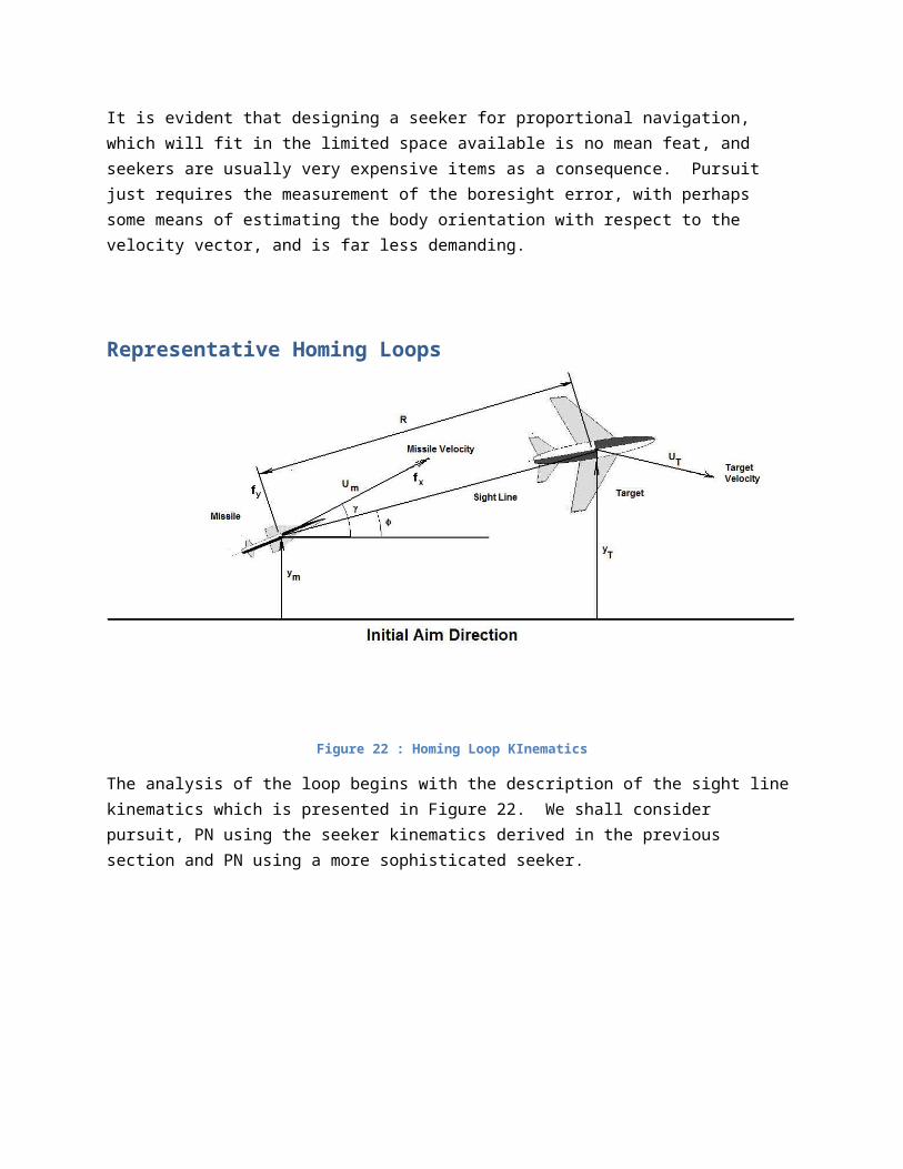
If the mass of the body is ‘m’ the inertial force is:

mu=F=T [m ( uB+ΩT uB )]Denoting the force measured in body axes FB:

F=TFB

So that the equation of (translational) motion becomes:

FB=m (uB+ΩT uB )

Inertial MomentsThe translational motion of the centre of gravity is of interest in calculating the flight path, but is by no means the complete story. In order to consider the rotation of the body to an angle of attack, we must address the response to moments, again generated in body axes.

We start by considering the motion of a particle at position xB=(x y z)T measured in the body frame with respect to some, as yet unspecified, reference point on the body. Its position in space is:

x=x0+Tx B

Where x0 is the position of the reference point.

The velocity of the particle is:

x= x0+T xB+T xB= x0+T xB

The body is rigid, so the particle does not move relative to the reference point.

Its inertial acceleration is:

x= x0+T xB

The inertial force becomes:

δF=δm ( x0+T xB )

Where δm is the mass of the particle.

Summing the components of force for all particles of the body:

F=m x0+∫ T xB dm

If we choose our reference point as the centre of gravity:

F=m xG=mu

And

∫ T xB=0

This means that for every particle accelerating in any particular direction, there is another accelerating in the opposite direction. In other words the sum of the internal forces of particles acting on each other within the rigid body is identically zero. If this were not the case, the body as a whole could be made to move by accelerating its internal components with respect to each other – which is nonsense.

So by referencing the motion to the centre of gravity we can treat the rotational motion independently of the translational motion.

The force acting on the particle, ignoring the force acting on the body as a whole, is:

δF=T xB δm

This is the same as the body axes force resolved into fixed axes:

δF=TδFB

i.e:

TδFB=T xB δm

Now: T=T ΩT

T=T ΩT+T ΩT=T (Ω2T+ΩT )

Therefore: δF B=(Ω2T +ΩT ) xB δm

A force Fx acting in the direction of the body x-axis, on the particle generates a moment Fx z about the pitch axis and –Fx y about the z-axis. The moments of the force acting on the particle at position (x,y,z) are:

( LMN )=( 0 −z y

z 0 −x− y x 0 )(Fx

F y

F z)

Where L,M and N are the roll, pitch and yawing moments. In matrix form:

Figure 40 : Moments due to X-wise Force

M B=XB FB

The Moment of the inertial force on the particle is therefore:

δM B=XB(Ω2T+Ω ) xB δm

Evaluating:

Ω2T+ΩT=(−q2−r2 pq−r pr+qpq+r −p2−r 2 qr− ppr−q qr+ p −p2−q2 )

(Ω2T+ΩT ) xB=(−x ( q2+r2)+ y ( pq−r )+ z ( pr+q )x ( pq+r )− y ( p2+r 2)+z (qr− p )x ( pr− q )+ y (qr+ p )− z ( p2+q2 ) )

X B(Ω2T +ΩT ) xB=(−zx ( pq+r )+zy ( p2+r 2)−z2 ( qr− p )+ yx ( pr−q )+ y2 (qr+ p )− yz ( p2+q2 )

−zx (q2+r 2)+zy ( pq−r )+z2 ( pr+q )−x2 ( pr−q )−xy (qr+ p )+xz ( p2+q2)xy ( q2+r2)− y2 ( pq−r )− yz ( pr+ q )+x2 ( pq+r )−xy ( p2+r2)+xz (qr− p ) )

=(( z2+ y2) p+( y2+ x2 ) qr−( z2+ x2 ) qr−xy ( q−pr )−zx ( r+ pq )− yz (q2−r2)( x2+z2) q+( z2+ y2 ) rp− ( x2+ y2) rp− yz ( r−qp )−xy ( p+qr )−zx (r 2− p2)( y2+ x2 ) r+( x2+z2) pq−( y2+z2) pq−zx ( p−rq )− yz ( q+rp )−xy ( p2−q2))

The moments depend on the six quantities:

A=∫ ( y2+z2) dmB=∫ ( z2+ x2 ) dmC=∫ ( x2+ y2 ) dmD=∫ zy dmE=∫ xz dmF=∫ yx dm

The first three are known as the moments of inertia, the remainder are called products of inertia. Rotational motion in space is more complex than the 2D case because the direction of the axis of rotation can change, whilst in 2D it is always fixed perpendicular to the plane of the motion.

For the whole body, the inertial moments become:

( LMN )=(A p−(B−C )qr−F ( q− pr )−D (q2−r2)−E ( r+ pq )

B q−(C−A )rp−D ( r−qp )−E (r 2− p2)−F ( p+qr )C r−( A−B ) pq−E ( p−rq )−F ( p2−q2)−D ( q+rp ))

The derivation involves less algebraic manipulation if we begin by considering the momentum of the particle:

δm u=δm T xB=δ mT ΩT xB

Expressed in body axes:

δm uB=δmΩT xB

The moment of momentum is:

δhB=XB ΩT xB δm

The angular momentum of the particle is found by evaluating this expression

δhB=( ( y2+z2) p−xyq−xzr−xyp+( x2+z2) q− yzr−xzp− yzq+( x2+ y2) r )δm

The total angular momentum of the body is:

hB=( A −F −E−F B −D−E −D C )( p

qr )=Jω

Where J is the inertia matrix and ω is the angular velocity.

Referred to fixed axes, the angular momentum is:

h=ThB

The rate of change of angular momentum (with respect to fixed axes) is equal to the applied moment:

M=h=T Jω+TJ { ω=TM B ¿

The body axes moments are then found from:

MB=ΩT Jω+J ω

This is much simpler to evaluate, and yields the same result.

Notice that our moment equations are derived by considering the translational motion of each particle of the body and summing the result. If any effects arise from the actual rotation of the individual particles, they would not be predictable from these equations.

The Inertia MatrixTo those familiar with motion in a plane, the moment of inertia terms should not be altogether unexpected. As with linear velocity, we should not be surprised that changes of orientation with respect to the angular momentum give rise to similar kinematic terms due to the changes in the projections of the angular momentum vector into body axes. From our experience with translational velocities in moving axes the pq,qr and rp kinematic terms are to be expected.

However the cross-axis products of inertia do not arise from either the change in angular momentum magnitude or change in body orientation with respect to the angular momentum, but because we have not specified the body reference axes with respect to the distribution of mass in the body. The equations have been derived for arbitrary distribution of mass.

To illustrate this point, consider the dumb-bell configuration of Figure 41. This consists of three equal masses in a straight line with the centre mass coincident with the origin (consistent with taking the centre of gravity as the reference point to avoid the introduction of translational forces into the moment equations). The configuration is oriented at angle θ with respect to the body-fixed reference axis. The moments of inertia of the individual masses with respect to the origin are not affected by the orientation of the body with respect to the chosen reference direction, so will be ignored.

Figure 41 : Illustration of Product of Inertia

At this orientation we find, for the inertia terms:

B=∫ ( x2+ y2) dm=m (a2 cos2θ+a2sin2θ+(−acosθ )2+(−asinθ )2

B=2ma2

The product of inertia F is:

F=∫ xy dx=2ma2 cosθ sin θ

The product of inertia depends on the orientation of the configuration with respect to the arbitrary choice of reference axes. Evidently, ‘F’ will be zero if θ=0.

Choosing the reference axes as axes of symmetry (as we might do automatically, as a matter of aesthetics,) the product of inertia, in this simple case at least, disappears.

More generally, consider the value of the inertia matrix in an axis set which is skewed with respect to this general axis set:

x p=TxB

The contribution of the general particle to the inertia matrix is:

δJ =(Ir2−x p x pT )δm

Where r is the distance from the cg to the particle. This is a vector magnitude which is invariant with respect to axis transformation.

This implies that the relationship between the old inertia matrix and the new is:

J p=TJ BT T

This is recognisable as a similarity transform. There exists an orientation for which the inertia matrix is diagonal . The elements are the eigenvalues of the arbitrary inertia matrix, and are called the principal moments of inertia (probably because the eigenvalues were once less pretentiously called the principal roots). The associated body axes are called principal axes, and they are usually obvious axes of symmetry. If the body is weirdly shaped they can be found from the eigenvalues, and the orientation from the eigenvectors, but normally they are obvious from inspection.

SimplificationIn deriving the moment equations we have ignored the fact that missiles usually exhibit considerable symmetry. By choosing the body axes to align with axes of symmetry of the configuration, all the products of inertia evaluate to zero, and the moment equations reduce to:

( LMN )

B

=( A p−( B−C ) qrB q−(C−A )rpC r−( A−B ) pq )

In this form they are known as Euler’s equation.

An important case in which a product of inertia must be taken into account is the analysis of aircraft dynamic stability. The aerodynamic forces on the aircraft are more conveniently referred to an axis system which is fixed with respect to the velocity vector, rather than the body longitudinal axis. With the aircraft an angle of attack, the product of inertia ‘E’ is no longer zero because the body is skewed with respect to the velocity vector, so that in aircraft stability work, the wind axes moment equations become:

( LMN )

w

=( A p−( B−C ) qr−E ( r+ pq )B q−(C−A ) rp−E (r2−p2)C r−( A−B ) pq−E ( p−rq ) )

However, the missile community usually only refers to aircraft in the context of ‘target’, so this is introduced as an interesting aside.

Perturbation FormThe equations do not lend themselves to straightforward analytical solutions, and the few cases which can be solved are to be found in the textbooks, so we add little to human knowledge by deriving them ourselves.

When designing control systems we are usually concerned with identifying equilibrium conditions corresponding to an input which is effectively steady state as far as the control loop of current interest is concerned. The issue is whether the system will remain at the given state once it reaches it. If, for whatever reason the deviation of the state from the desired value becomes large, it is by definition a poor controller.

In nature systems evolve to be highly non-linear to the extent that equilibia become impossible to define, and the systems evolve to a state of perpetually changing goals, so that the observed behaviour is usually chaotic.

Economists appear to delude themselves that they can derive laws which govern systems which are intrinsically chaotic. The stability of the equilibrium of the supply/demand curves has yet to be analysed, and there is a suspicion that markets are inherently unstable and short-lived unless regulated by central authority or rigged by crooks. Yet their pontifications encourage the abandonment of morality and wisdom in the name of the great god of supply and demand. Heretics are ridiculed as foolish and ignorant, with a fervour which is religious in its intensity. Priests and soothsayers have always had the ear of those in power in preference to the mere artisan. That goes a long way to explain the mess we are in.

However, it does give rise to a world where there is a depressingly high demand for guided weapons.

In an artificial system, we have control over the information flows and can even revert to redesign of the hardware if it really is a sow’s ear to control. We are concerned with small changes in the equilibrium states (perturbations which are sufficiently small for second order terms to be ignored.

In aircraft applications, the equilibrium state of trim at an angle of attack is the same for all flight conditions, because the variation in equilibrium angle of attack is accounted for in the product of inertia which is present in the version of the equations of motion used.

Missiles require a much more diverse range of equilibrium conditions. On the other hand, the trajectory of a missile is determined by the navigation law, so that unlike aircraft, the long term modes such as

Phugoid and spiral divergence are pretty well irrelevant. Once the guidance fails, the missile usually self destructs, a behaviour, which is not to be recommended for aircraft.

The equations of motion referred to body axes are:

X=m ( u+wq−vr )Y=m ( v+ur−wp )Z=m ( w+vp−ur )

Where X, Y and Z are the components of force, and m is the mass. The moment equations are:

L=A p−(B−C )qrM=B q−(C−A ) rpN=C r−( A−C ) pq

The x-wise equation has very little influence on the short period modes relevant to the autopilot, and can be neglected.. For a Cartesian missile the yaw and pitch behaviour is identical, so only one lateral force and one lateral moment equation need be considered. Also, B=C and the roll rate is small, so the equations reduce to:

Y=m ( v+Ur )N=C rL=A p

The product ur remains because the speed of the missile is not a small quantity, to emphasise the point an upper case U has been used.

This is the basic form representing behaviour at small angles of attack, which is the usual starting point.

Unlike aircraft, missiles may reach very high angles of attack (σ). During the vertical launch manoeuvre, this can even reach 90˚ (i.e. the missile flying sideways). We have:

u=U cosσ

v=U sin σ

The x-wise equation cannot be ignored:

X=m ( u−U sin σ r )Y=m ( v+U cos σ r )N=C rL=A p

The other common form is with the missile spinning.

The equations of motion become:

Y=m ( v+Ur−wP )Z=m ( w+vP−Uq )M=B q−(C−A ) rPN=C r−( A−B ) Pq

CommentSome might say that this presentation is rather long-winded, after all, the equations can be written down in a few lines using Lagrangian methods. However, the aim of the game is to impart understanding, and there is much about the motion in three dimensions, referred to body axes, which is counter-intuitive to those having dealt only with 2D motion.

Al too often the skill in manipulating equations is mistaken for actual understanding of the behaviours represented by them. Whilst this is acceptable, even required, of a mathematician, it is anathema to the engineer.

Autopilot Basics 2 – Aerodynamic Forces

IntroductionThe inertial forces expressed in body axes introduce cross-product terms, arising from the changes in orientation with respect to the velocity and angular momentum vectors.

The forces which control the motion of the missile arise from the pressure distribution over the body which is a far from trivial exercise to predict. So to characterise them for our purposes, we use linear small perturbation approximations to the changes in forces and moments in response to perturbations in the current equilibrium state.

The region over which the linear approximation is adequate must be known, as this will be one of the factors which determines the tightness of control required. An airframe which exhibits sudden changes in flow regime probably needs to be sent back to the aerodynamicists, to think again.

Stability DerivativesThe missile moves under the influence of three forces and three moments, which depend on the state variables and their time derivatives.

F=(X (u , v ,w , p ,q , r ,u , v , w )Y (u , v ,w , p , q , r , u , v , w )Z (u , v , w , p , q , r ,u , v , w )L (u ,v , w , p , q , r ,u , v , w )M (u , v , w , p ,q , r ,u , v , w )N (u , v ,w , p ,q , r , u , v , w )

)We are interested in the behaviour in the vicinity of equilibrium positions, where linear approximations apply, e.g:

ΔX=∂ X∂u

Δu+∂ X∂ v

Δv+…

In the context of designing autopilots, the Δs are usually omitted from the notation, because it is understood that we are dealing with perturbations. Also it is universal practice to replace the partial derivative notation with the more compact notation of using a subscript to denote the independent variable, for example:

∂ X∂u

=Xu , ∂ X∂ v

=X v , …

The partial derivatives written in this form are called stability derivatives. Except at high angles of attack, the x-wise forces are usually irrelevant, and most of the other derivatives are negligible on account of the symmetry. In missile applications the important derivatives are:

Yaw channel: Y v , N v , N r

Pitch channel: Zw , M w , M q

Roll channel; Lp

Force Derivatives Yv and Zw

Figure 42 : lateral Forces

When flying at constant speed, the body axes components of velocity are the projections of the velocity vector on to body axes. For small angles of attack, the orientation is defined as two orthogonal angles α and β in the pitch and yaw planes respectively. However for large angles of attack, which are commonplace in missile motion, it is usual to define the orientation of the plane containing the body x-axis and the velocity vector with respect to the body x-z plane. This is the aerodynamic roll angle, not to be confused with the Euler roll angle, which is the orientation with respect to inertial axes.

From Figure 42, a nose up displacement (positive w) will generate an upwards force, which in the z-down axis system employed is a negative force. Consequently, Zw will be negative. Similarly for Yv. In a cruciform missile:

Y v=Zw

Aerodynamic ‘Stiffness’ Nv and Mw

In Figure 42, the lift force acts behind the centre of gravity so a change in angle of attack generates a nose-down moment, tending to cancel the disturbance causing the displacement. The missile is statically stable. The derivative Mw is therefore negative for a statically stable missile. However, missiles may be stabilised by virtue of feedback control in the autopilot, so statically unstable airframes with positive Mw are possible.

In the yaw plane positive angle of attack causes an anti-clockwise moment, so for static stability Nv is positive.

These two derivatives characterise the tendency of the airframe to point in the direction of flight, rather like a weather-vane pointing into the wind.

For a cruciform missile:

M w=−N v

Damping – Lp, Mq and Nr

As the body rotates, the lifting surfaces move laterally with respect to the airflow so that the local angle of attack differs from that of the configuration as a whole, and forces are generated. As the forces act away from the centre of gravity, they generate moments. All damping derivatives are negative, as they oppose the motion causing them. Also for a cruciform missile:

M q=N r

CommentThose from an aircraft background may be surprised at the simplicity of description of the missile aerodynamic behaviour. Aircraft practice introduces derivatives which are not relevant to missiles largely because the design objectives are different. Traditionally, aircraft stability was directed to designing aircraft which were well behaved and pleasant to fly by virtue of their natural stability and response. Missiles invariably have closed loop autopilots which are extremely robust to uncertainties in the plant model used to design them, and can get away with a fairly simple representation of the aerodynamics as a consequence.

ControlThe stability derivatives determine the motion of an unguided rocket in response to disturbances, but additional forces and moments are needed for steering to be possible.

The control takes the form of deflecting surfaces with respect to the airflow by means of actuators, and a lot of ingenuity has been invested into actuator design, but we shall assume a cruciform configuration in which the control surfaces lie in the wing planes.

The pitch control uses either deflection of the tail, or of forward mounted surfaces called ‘canards’.

In a statically stable missile, the trim lift of the canard control acts in the same direction as the control lift, which reduces the angle of attack for a given lateral force compared to tail control. However, it places the control at a higher angle of attack than the missile as a whole, so loses effect at high angles of attack. Also the flow field from the canards affects the behaviour of the wings, which in missiles invariably means unpredictable roll control. For this reason, the main wings of canard controlled missiles are usually mounted on a bearing to rotate freely in roll.

Tail control does not suffer from this aerodynamic interaction, and trims with the control at a lower angle of attack compared with the configuration as a whole. However, it is easier to package servos in the fore body of a missile than it is at the rear which is invariably occupied by a rocket motor. The trade-offs are subtle, but in the author’s experience, it is a matter of the culture of the particular manufacturer rather than a consequence of a system optimisation.

The control deflection perturbations are denoted ξ, η and ζ for roll pitch and yaw respectively (xi, eta, zeta). The corresponding derivatives are:

Force: Y ζ Zη

Moment: Lξ M η N ζ

In a moving wing missile, the force terms dominate, as the total lift is generated by rotating the wings with respect to the airflow, whilst the tail serves to point the body into wind. In contrast, tail and canard control missiles seek to minimise the force term.

The convention chosen is that positive control deflections cause positive body moments.

Equations of MotionThe small perturbation equations for a non-spinning missile, with respect to a trim condition, become:

(Y v

m )v+(Y ζ

m )ζ= v+Ur

(N v

C )v+(N r

C )r+(N ζ

C )ζ =q

(Lp

A ) p+(Lξ

A )ξ= p

Note that at high angles of attack, perturbations in body x-wise velocity become significant (i.e. Yu, Nu may need to be considered).

Before considering how to design autopilots, we consider the natural motion of the missile, without feedback. If this is adequate, there is no requirement for expensive controllers. Indeed, it is the understanding of the natural motion that yields the clues to solving the problem of autopilot design.

We need to know what is wrong with the behaviour before we seek to correct it. ConfuseUs he say; better understand question before seeking answer.

Note that we have already used our engineering understanding of the problem to justify extracting the high frequency weather-vane behaviour from the trajectory modes. Any pilot will tell you that an aircraft with short period oscillation and phugoid motion having similar frequencies would be just about impossible to fly. Yet time and again I come across the recommendation to use Butterworth pole patterns by people who ought to know better.

The transfer functions relating incidence and body rate to control deflection become:

vζ=

Y ζ

ms−(Y ζ

mN r

C+

N ζ UC )

s2−( Y v

m+

N r

C )s+( Nv UC

+Y v

mN r

C )

rζ=

N ζ

Cs−(Y v

mN ζ

C−

Y ζ

mNv

C )s2−( Y v

m+

N r

C )s+( Nv UC

+Y v

mN r

C )We see straight away that the characteristic equation is:

s2−( Y v

m+

N r

C )s+( N v UC

+Y v

mN r

C )=0The motion corresponding to this equation is known as the weather-vane response (in deference to our American cousins who appear to be offended by ‘weather-cock’, for some reason). It order to ensure guidance loop stability, the characteristic frequency (the weather-vane frequency) must be high – usually between 1/3rd and 1/10th that of the guidance loop to ensure adequate decoupling of the associated modes.

The natural frequency is:

ωn=√ Nv UC +

Y v

mN r

C

Note for static stability Nv is positive and Yv and Nr are both always negative. The damping term is therefore always positive.

In order to make this high using the natural stability, we find that the damping term becomes small. It is usually impossible to achieve the desired weather vane frequency by airframe design without simultaneously reducing the damping.

One solution, which has been adopted for small, low cost missiles is the place a notch filter between the acceleration command input and the servo:

ζf yd

=s2+(Y v

m+

N r

C ) s+( N v UC

+Y v

mN r

C )s2+2 ζ n√ N vU

C +Y v

mN r

C +( N vUC +

Y v

mN r

C )

Here the ζn in the transfer function refers to the desired damping ratio of the weathervane mode. This is an example of an open-loop, ‘feed forward’ controller. It can only damp out disturbances arising from the input signal, but is vulnerable to disturbances from any other source. Before using this type of controller, the designer must be satisfied that disturbance rejection is adequate. Also the notch filter characteristics need to be varied with flight regime, and the notch never exactly matches the true weather-vane frequency.

We note also that the system possesses transmission zeros, e.g for the incidence response:

s−( N r

C+ m

Y ζ

N ζ UC )

The damping term, Nr is usually insignificant compared with the control derivatives.

Figure 43 : Reverse Action effect of Tail Control

For a canard configuration, the control acts ahead of the centre of gravity so the control force is in the positive direction for positive yaw. The zero is located in the left hand half plane. For a tail controlled missile, positive yaw requires a control force in the negative direction, and the zero is in the right hand half plane. Large tail surfaces with a small moment arm may result in large Nv (i.e. high weather-vane stiffness) but moves this zero close to the imaginary axis, severely restricting the achievable closed loop bandwidth.

The zero arises from the lateral force due to the control. In a tail controlled missile this acts in the opposite sense to the desired lift. Initially the lift is in the wrong direction until the body rotates to its angle of attack.

The position of zeros is inherent in the dynamics of the plant, and cannot be moved by controller design, nor can a right half plane zero be cancelled with an RHP pole without introducing the unstable mode associated with the RHP pole.

It has been suggested that taking the reference point as other than the centre of gravity, these zeros can be changed. That is not the case. Changing the reference point requires all the force terms which were eliminated by choosing the centre of gravity as reference must be re-introduced. The equations become horrifically complicated, but the zero position does not change one iota. If the additional force terms are not re-introduced, the equations are simply wrong.

Before moving on to closed loop controller options, we shall consider what happens when the missile is allowed to spin. We shall consider the open loop case with zero control input, and will ignore the pitch and yaw damping derivatives Mq and Nr, they are rarely very large in missile configurations anyway.

The equations of motion become:

Y v v=m ( v+Ur−wP)Zw w=m (w+vP−Uq )M w w=B q−(C−A ) rPNv v=C r−( A−B ) Pq

For a symmetrical cruciform missile:

Zw=Y v

Mw=−N vB=C >> A

The characteristic equation is a quartic, which factorises into the two terms:

s2−Y v

ms+

N v UB

+ p2± p√4 N v UB

−(Y v

m )2

=0

Denoting the weathervane frequency ωn and damping ratio ζn, we have from the weathervane characteristic equation (without the damping derivative):

ωn2=

N v UB

2 ζ n ωn=Y v

m

The constant term, characterising the weathervane stiffness may be written more compactly as:

a0=ωn2+p2±2 pωn√1−ζn

2

This has its minimum value at a spin rate:

p=ωn √1−ζn2

This is recognisable as the resonant frequency. However, the constant term only becomes zero if the damping ratio is zero, its minimum value is:

a0=ωn2 ζ n2

So the body axes components of velocity vary sinusoidally with frequency ωnζn whilst the body rotates at p. The pitch/yaw motion is perpendicular to the roll motion. The missile conducts a tight barrel roll having an angular velocity magnitude:

ω2=a0+ p2=ωn2 ζn2+ωn

2 (1−ζ n2)=ωn

2

The very low stiffness renders the missile vulnerable to disturbances, so that very high angles of attack can be reached.

AutoPilot Basics 3

IntroductionWe have derived the governing equations of motion and considered how a missile will behave without any feedback control. Sometimes adequate bandwidth can be realised from the aerodynamic design alone, especially if the missile is small. More typically, the penalty for high weathervane frequency is either excessive reverse action, poor damping and low trim incidence. Rapid, well-behaved response is usually only achievable with some form of feedback control.

This chapter examines the more common autopilot structures.

Some improvement over the natural missile behaviour may be achieved by ingenious devices such as the rolleron, depicted in Figure 44.

Figure 44: Rolleron Schematic

The rolleron is a way of augmenting the weathervane and roll damping without the complication and expense of an instrumented autopilot. A gyro rotor is spun by the airflow. When the missile pitches, gyroscopic torques proportional to the body rate cause the gyro to precess, deflecting a flap which generates a pitching moment opposing the body rotation.

Improving the DampingIt is often possible to achieve the necessary bandwidth but at the cost of poor weathervane damping. The next option terms of complexity, above the notch filter feed forward autopilot, uses rate gyro feedback to overcome this particular vice.

Figure 45 : Rate Loop, Ignoring Servo Response

The zero in the rate response is located in the left half plane, so augmenting the damping by rate feedback is reasonably straightforward.

However, it is to be noted that the output from the autopilot is lateral acceleration:

f y=v+Ur

So the transfer function relating lateral acceleration to control deflection is:

f y

ζ=s v

ζ+U r

ζ

The control loop from lateral acceleration demand input to the achieved lateral acceleration is presented in Figure 46. The incidence and body rate are changing at the same time. As the denominators of their respective transfer functions are the same, we might expect the incidence and body rate response times to be similar. However, the dynamics of the problem indicate that they cannot possibly respond to the control input equally quickly, the body must first start to rotate before the incidence can build up.

Figure 46 : Rate Loop - Latax response

Incidence LagThe difference in responses is attributable to the zeros of the two transfer functions. To illustrate this, we construct a mythical transfer function relating lateral acceleration to body rate. This is not a causal relationship but merely a ploy to illustrate the effect of the transfer function zeros:

f y

r=

f y

ζζr

The latax response is:

f y

ζ=

Y ζ

ms2−

Y ζ

mN r

C−(Y v

mN ζ

C−

Y ζ

mNv

C )Us2−(Y v

m+

N r

C )s+(N v UC

+Y v

mN r

C )We see that the input to this transfer function is directly linked to the output. This is because the control immediately generates a lateral force when it is deflected.

f y

r=

Y ζ

ms2−

Y ζ

mN r

Cs−( Y v

mN ζ

C−

Y ζ

mN v

C )U

N ζ

Cs−(Y v

mN ζ

C−

Y ζ

mN v

C )The numerator is of higher order than the demoninator, so this is not a realisable response, its purpose is to illustrate the effects of the phase lags introduced by the zeros.

Having a large reverse-action effect is undesirable, so we should aim to design the airframe such that Y ζ is small. Also, since we are adding rate feedback specifically to improve the weather-vane damping, it is a reasonable assumption that the natural damping (Nr) is insignificant. Setting these derivatives to zero:

f y

Ur= 1

1− mY v

s

Now Ur is the value of lateral acceleration, once the incidence has reached its steady state. So this transfer function characterises how much more slowly the incidence builds up compared with the body rate.

The quantity

mY v is usually called the ‘incidence lag’ because it characterises how the incidence lags

behind the body rate. It isn’t a true lag, merely a characterisation of the ratio of the zeros of the two governing transfer functions.

Lateral Acceleration FeedbackIf rate feedback alone is insufficient to ensure the response is adequate, it will be necessary to feedback the quantity we actually wish to control – the lateral acceleration. This changes the system from single input/single output to a multiple output system. There have been all styles of Emperor’s New Clothes generated by academia over the past forty years, but there is little to beat a thorough understanding of the dynamics of the specific system under consideration, and old fashioned SISO methods.

There is plenty of arcane literature around, and the practitioner really needs to know whether the effort involved in acquiring the current esoteric fad is commensurate with the practical benefits. I will merely say, I’ve been there - don’t bother.

Figure 47 : Nested Loops

The trick is to treat the system as a series of nested loops, so that at any time we are dealing with a SISO system. Our derivation of the transfer function relating latax to body rate enables us to design the

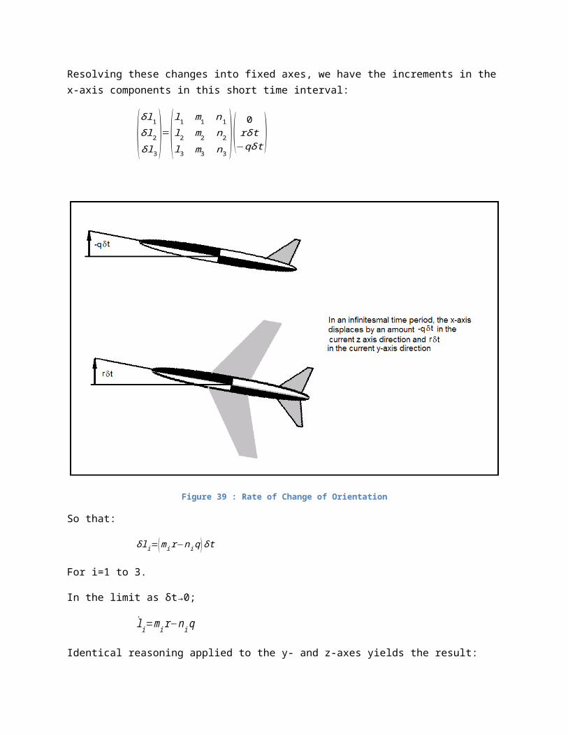
autopilot as a pair of nested loops, the inner loop being the rate loop, the outer loop the acceleration feedback loop. This is depicted in Figure 47.

In order to avoid excessive clutter, we shall assume that Nr and Yζ are insignificant. In a closed loop system, we know are plant equations are approximations, after all that is one of the reasons why we close the loop.

The closed rate loop transfer function becomes:

G (s )=K r

N ζ

C (s−Y v

m )s2+(K r

N ζ

C−

Y v

m ) s+( N v UC

−K r

Y v

mN ζ

C )We see from the denominator that the damping is modified. The zero is in the left half plane, so represents phase advance, which is a desirable feature from a stability perspective.

However is we feed a constant input into the loop:

r (t )=r D→r D

s

We notice the steady state output (s→0), is:

rout (s )→−K r

N ζ

CY v

mN v U

C −K rY v

mN ζ

C

r D

s

The output is constant, but not equal to the input. We could pre-multiply the input by the reciprocal of this gain, but since the parameters are not known accurately, this would introduce a {much smaller} error. In any case feed forward is usually a bad idea, because it is much more vulnerable to plant uncertainties and disturbances compared with feedback.

The simplest control solution is to get the aerodynamicists to design the missile to have near neutral static stability, i.e Nv≈0. This yields unity steady state gain.

To the novice it comes as a surprise that a loop designed on the basis of stability does not also have adequate tracking properties. The simplest explanation is that stability deals with the impulse response of the system, so that if the impulse response of G(s) is satisfactory it does not follow that when we feed it with a time varying input:

yin ( t )= y D tn→y D

sn+1

that the solution will converge to zero as time progresses. We are designing the loop with the wrong transfer function. Our open loop description must correspond to the impulse response of the system fed by the expected input, i.e:

G0 ( s)=G ( s)sn+1

If the input is anything other than an impulse, the stability analysis will be insufficient to ensure adequate tracking properties, and additional integrators will be required within the loop. On many occasions, G(s) itself contains integrators, so they do not need to be added explicitly in the compensation.

This argument applies equally to the frequency domain where our transfer function is the Fourier transform of the time domain impulse response. We must reduce our system description to an impulse response before we can begin to apply control theory.

It follows that, if the missile cannot maintain neutral stability under all flight conditions, or if it relies on its natural static stability to achieve its bandwidth, the loop must contain integral feedback.

Our feedback gain, at the very least, must contain an integrator:

K r=kr+kI

s

This yields the transfer function:

rζ=

N ζ

C (kr s+k I ) (s−Y v

m )s3+( N ζ

Ckr−

Y v

m )s2+( Nζ

Ck I−

N ζ

CY v

mk r+

Nv UC )s−k I

Y v

mNζ

C

We see that this does indeed yield a unity steady state gain.

Concluding CommentI have no intention of proceeding with an autopilot design as such; there are plenty of text books on control, and myriad methods which can be employed to calculate feedback gains and design compensators. I have little to add.

The basis of all control system design is a thorough understanding of the behaviour of the plant to be controlled, not skill in manipulating abstract matrices, as appears to be the current premise. It is precisely this understanding, which is conspicuous by its absence from many modern texts, and indeed, from many learned papers on the subject.

A word of warning: All too often I see the recommendation to use Butterworth pole patterns, and I have already commented on the disastrous effect that would have on an aircraft stability quartic. Modal separation in frequency is the most powerful single tool available to the control engineer, it allows us to consider each mode in isolation, effectively factorising the characteristic equation on the basis of understanding of the dynamics.

If modal separation is impossible, i.e. if all modes do indeed have identical frequency, I should have serious doubts as to whether the plant is fundamentally fit for purpose. It certainly makes no sense to force them all to the same frequency.

Remember the missile dynamics is characterised by the weathervane mode and the incidence lag. Design autopilots with that knowledge in the back of your mind, at you won’t go far wrong.