Introduction - Vrije Universiteit Brusselhomepages.vub.ac.be/~scaenepe/groupcorings7.pdf · We introduce group corings, ... in fact there is a categorical correspondence ... functors

GROUP CORINGS

S. CAENEPEEL, K. JANSSEN, AND S.H. WANG

Abstract. We introduce group corings, and study functors betweencategories of comodules over group corings, and the relationship tograded modules over graded rings. Galois group corings are defined,and a Structure Theorem for the G-comodules over a Galois group cor-ing is given. We study (graded) Morita contexts associated to a groupcoring. Our theory is applied to group corings associated to a comodulealgebra over a Hopf group coalgebra.

Introduction

Group coalgebras and Hopf group coalgebras were introduced by Turaev[15]. A systematic algebraic study of these new structures has been carriedout in recent papers by Virelizier, Zunino, and the third author (see forexample [16, 17, 18, 19, 21, 22]). Many results from classical Hopf algebratheory can be generalized to Hopf group coalgebras; this has been explainedin a paper by the first author and De Lombaerde [6], where it was shownthat Hopf group coalgebras are in fact Hopf algebras in a suitable symmetricmonoidal category.In [20], the third author investigated how Hopf-Galois theory can be devel-oped in the framework of Hopf group coalgebras. A definition of Hopf-Galoisextension was presented; the requirement is that a set of canonical maps,indexed by the elements of the underlying group, has to be bijective. Oneaspect in the present theory that is not satisfactory is the lack of an appro-priate Structure Theorem: an important result in Hopf-Galois theory statesthat the category of relative Hopf modules over a faithfully flat Hopf-Galoisextension is equivalent to the category of modules over the coinvariants. Sofar, no such result is known in the framework of Hopf group coalgebras.Corings were introduced by Sweedler [14], and were revived recently byBrzezinski [3]. One of the important observations is that coring theory pro-vides an elegant approach to descent theory and Hopf-Galois theory (see

2000 Mathematics Subject Classification. 16W30, 16W50.Key words and phrases. Corings, group coalgebras, Hopf-Galois extensions, graded

rings, graded Morita contexts.This research was supported by the research project G.0622.06 “Deformation quantiza-

tion methods for algebras and categories with applications to quantum mechanics” fromFWO-Vlaanderen. The third author was partially supported by the SRF (20060286006)and the FNS (10571026).

1

2 S. CAENEPEEL, K. JANSSEN, AND S.H. WANG

[3, 4, 5]). The aim of this paper is to develop Galois theory for group cor-ings, and to apply it to Hopf group coalgebras.A G-A-coring (or group coring) consists of a set of A-bimodules indexed bya group G, together with a counit map, and a set of diagonal maps indexedby G ×G, with appropriate axioms (see Section 1). A first remarkable ob-servation is the fact that we can introduce two different types of comodulesover a group coring C. C-comodules consist of a single A-module, with aset of structure maps indexed by G, while G-C-comodules consist of a set ofA-modules indexed by G, together with structure maps indexed by G×G.We have a pair of adjoint functors between the two categories of comodules(see Proposition 1.1). This remarkable fact can be explained by duality ar-guments. Dualizing the definition of a G-A-coring, we obtain G-A-rings; inthe coalgebra case, this was observed in [21]. In contrast to G-corings, G-rings are a well-known concept: in fact there is a categorical correspondencebetween G-A-rings and G-graded A-rings. The graded ring correspondingto a G-ring is the so-called “packed form” of the G-ring, in the terminologyof [21]. We don’t have a similar correspondence between group corings andgraded corings, unless the group G in question is finite. This indicates thatduality properties for module categories over graded rings have to be studiedfrom the point of view of group corings, rather than graded corings.Over a graded ring, one can study ordinary modules and graded modules,and there exists an adjoint pair between the two categories. We also havefunctors from the categories of C-comodules (resp. G-C-comodules) to mod-ules (resp. graded modules) over the dual graded ring of C. All thesefunctors appear in a commutative diagram of functors (see Proposition 4.5).The functor between the category of G-C-comodules and graded modules isan equivalence if every Cα (or equivalently, every homogeneous part of thedual graded ring) is finitely generated and projective as an A-module (seeProposition 4.4). These properties of (co)module categories are studied inSections 1, 3 and 4.An important class of group corings, called cofree group corings, is investi-gated in Section 2. Basically, these are corings for which all the underlyingbimodules are isomorphic. A cofree coring is - up to isomorphism - de-termined by Ce, its part of degree e; its left dual is the group ring ∗Ce[G]over the left dual of Ce (Proposition 4.6). The category of G-C-comodules isequivalent to the category of comodules over Ce (Theorem 2.2). This is ananalog of the well-known fact that, for a group ring R[G], the category ofgraded R[G]-modules is equivalent to the category of R-modules.In Section 5, we introduce the notion of grouplike family of a group coring.Grouplike families correspond bijectively to C-comodule structures on A.Fixing a grouplike family, we can introduce the coinvariant subring T of A.We have two pairs of adjoint functors, one connecting modules over the coin-variants to right C-comodules (Proposition 5.3), and another one connectingmodules over the coinvariants to right G-C-comodules (Proposition 5.4). Itcan be established when the latter adjoint pair, denoted (F7, G7), is a pair

GROUP CORINGS 3

of inverse equivalences. Given a group coring C with a fixed grouplike fam-ily, we can define a canonical morphism of group corings between the cofreecoring built on the Sweedler canonical coring and the coring C. If F7 isan equivalence, then this canonical morphism is an isomorphism (Proposi-tion 5.7). In this case, we call our group coring a Galois group coring. Thisis equivalent to C being cofree, and Ce being a Galois coring. The StructureTheorem 5.12 is our main result. Basically, if C is Galois, and A is faithfullyflat over the coinvariants, then F7 is an equivalence.Morita theory plays an important role in this theory. To a group coring witha fixed grouplike family, we can associate several Morita contexts. Two ofthem are classical Morita contexts, and have been studied in a special sit-uation (see Section 10) in [20]. But the natural Morita contexts are in factgraded Morita contexts. In Section 6, we give some generalities on gradedMorita contexts; in Sections 7 and 8, we discuss the Morita contexts andtheir relationship.In some situations, the Galois property of a group coring can be charac-terized by the graded Morita contexts associated to it. We study this inSection 9. In the final Section 10, we briefly discuss the situation where C isa group coring A⊗H associated to a right H-comodule algebra A, where His a Hopf group coalgebra, as introduced in [15]. We show that this groupcoring is Galois if and only if A is an H-Galois extension in the sense of [20].This entails a Structure Theorem for relative group Hopf modules; we alsodescribe the dual of the group coring A⊗H.

Throughout this paper, we will adopt the following notational conventions.For an object M in a category, M will also denote the identity morphismon M .Let G be a group and M a (right) A-module. We will often need collectionsof A-modules isomorphic to M and indexed by G. We will consider thesemodules as isomorphic, but distinct. Let M×{α} be the module with indexα. We then have isomorphisms

µα : M →M × {α}, µα(m) = (m,α).

We can then write M × {α} = µα(M). µ can be considered as a dummyvariable, we will also use the symbols γ, ν, . . .. We will identify M andM × {e} using µe.

1. Group corings and comodules

Let G be a group, and A a ring with unit. The unit element of G will bedenoted by e. A G-group A-coring (or shortly a G-A-coring) C is a family(Cα)α∈G of A-bimodules together with a family of bimodule maps

∆α,β : Cαβ → Cα ⊗A Cβ ; ε : Ce → A,

such that

(1) (∆α,β ⊗A Cγ) ◦∆αβ,γ = (Cα ⊗A ∆β,γ) ◦∆α,βγ


and

(2) (Cα ⊗A ε) ◦∆α,e = Cα = (ε⊗A Cα) ◦∆e,α,

for all α, β, γ ∈ G. We use the following Sweedler-type notation for thecomultiplication maps ∆α,β:

∆α,β(c) = c(1,α) ⊗A c(2,β),

for all c ∈ Cαβ . Then (2) takes the form

(3) c(1,α)ε(c(2,e)) = c = ε(c(1,e))c(2,α).

(1) justifies the following notation:

((∆α,β⊗ACγ)◦∆αβ,γ)(c) = ((Cα⊗A∆β,γ)◦∆α,βγ)(c) = c(1,α)⊗Ac(2,β)⊗Ac(3,γ),for all c ∈ Cαβγ . If C is a G-A-coring, then C = Ce is an A-coring, withcomultiplication ∆e,e and counit ε.A morphism between two G-A-corings C and D consists of a family of A-bimodule maps (fα)α∈G, fα : Cα → Dα such that

(fα ⊗A fβ) ◦∆α,β = ∆α,β ◦ fαβ and ε ◦ fe = ε.

If A is a commutative ring, and ac = ca, for all α ∈ G, a ∈ A and c ∈ Cα,then C is called a G-coalgebra, cf. [15].

Over a group coring, we can define two different types of comodules. A rightC-comodule is a right A-module M together with a family of right A-linearmaps (ρα)α∈G, ρα : M →M ⊗A Cα, such that

(4) (M ⊗A ∆α,β) ◦ ραβ = (ρα ⊗A Cβ) ◦ ρβand

(5) (M ⊗A ε) ◦ ρe = M.

We use the following Sweedler-type notation:

ρα(m) = m[0] ⊗A m[1,α].

(4) justifies the notation

((M ⊗A ∆α,β) ◦ ραβ)(m) = ((ρα ⊗A Cβ) ◦ ρβ)(m) = m[0] ⊗Am[1,α] ⊗Am[2,β],

and (5) is equivalent to m[0]ε(m[1,e]) = m, for all m ∈M .A morphism of right C-comodules is a right A-linear map f : M → Nsatisfying the condition

(6) (f ⊗A Cα) ◦ ρα = ρα ◦ f,

for all α ∈ G. MC will be our notation for the category of right C-comodules.

A right G-C-comodule M is a family of right A-modules (Mα)α∈G, togetherwith a family of right A-linear maps

ρα,β : Mαβ →Mα ⊗A Cβ

GROUP CORINGS 5

such that

(7) (Mα ⊗A ∆β,γ) ◦ ρα,βγ = (ρα,β ⊗A Cγ) ◦ ραβ,γand

(8) (Mα ⊗A ε) ◦ ρα,e = Mα

for all α, β, γ ∈ G. We now use the following Sweedler-type notation:

ρα,β(m) = m[0,α] ⊗A m[1,β],

for m ∈Mαβ . (7) justifies the notation

((Mα ⊗A ∆β,γ) ◦ ρα,βγ)(m) = ((ρα,β ⊗A Cγ) ◦ ραβ,γ)(m)= m[0,α] ⊗A m[1,β] ⊗A m[2,γ],

for m ∈ Mαβγ . (8) implies that m[0,α]ε(m[1,e]) = m, for all m ∈ Mα. Amorphism between two right G-C-comodules M and N is a family of rightA-linear maps fα : Mα → Nα such that

(fα ⊗A Cβ) ◦ ρα,β = ρα,β ◦ fαβ .The category of right G-C-comodules will be denoted by MG,C .

Proposition 1.1. We have a pair of adjoint functors (F1, G1) between thecategories MG,C and MC. Moreover, if G is a finite group, then (F1, G1) isa Frobenius pair of functors, i.e. F1 is also a right adjoint of G1.

Proof. Take M = (Mα)α∈G ∈MG,C , and define

F1(M) =⊕α∈G

Mα = M.

The coaction maps ρα : M →M ⊗A Cα are defined as follows: for m ∈Mβ,let

(9) ρα(m) = m[0,βα−1] ⊗A m[1,α].

Otherwise stated, ρα =⊕

β∈G ρβα−1,α. Let us show that (4,5) hold. For allm ∈Mγ , we compute that

((ρα ⊗A Cβ) ◦ ρβ)(m) = (ρα ⊗A Cβ)(m[0,γβ−1] ⊗A m[1,β])= m[0,γβ−1α−1] ⊗A m[1,α] ⊗A m[2,β]

= ((M ⊗A ∆α,β) ◦ ραβ)(m);((M ⊗A ε) ◦ ρe)(m) = m[0,γ]ε(m[1,e]) = m.

For a morphism f : M → N in MG,C , we simply define

F1(f) =⊕α∈G

fα.

Let us now define G1. For M ∈ MC , let G1(M)α = µα(M), where we usethe notation introduced at the end of the introduction. The coaction mapsρα,β : µαβ(M) → µα(M)⊗A Cβ are defined by

(10) ρα,β(µαβ(m)) = µα(m[0])⊗A m[1,β],


for all m ∈M . The formulas (7,8) hold since

((Mα ⊗A ∆β,γ) ◦ ρα,βγ)(µαβγ(m))= (Mα ⊗A ∆β,γ)(µα(m[0])⊗A m[1,βγ])

= µα(m[0])⊗A m[1,β] ⊗A m[2,γ]

= ρα,β(µαβ(m[0]))⊗A m[1,γ]

= ((ρα,β ⊗A Cγ) ◦ ραβ,γ)(µαβγ(m));((Mα ⊗A ε) ◦ ρα,e)(µα(m))

= (Mα ⊗A ε)(µα(m[0])⊗A m[1,e])

= µα(m[0])ε(m[1,e]) = µα(m[0]ε(m[1,e])) = µα(m).

On the morphisms, G1 is defined as follows: for f : M → N in MC , we put

G1(f) = (να ◦ f ◦ µ−1α )α∈G.

Take M ∈MG,C and N ∈MC , and consider the map

ψ : HomC(F1(M), N) → HomG,C(M,G1(N))

defined as follows. For f :⊕

α∈GMα → N , let

ψ(f)α = να ◦ f ◦ iα : Mα → G1(N)α = να(N),

where iα : Mα →⊕

α∈GMα is the canonical injection. Now consider themap

φ : HomG,C(M,G1(N)) → HomC(F1(M), N),

defined as follows: for g = (gα)α∈G : M → G1(N), let

φ(g)(m) =∑α∈G

(ν−1α ◦ gα ◦ pα)(m),

where now pα :⊕

α∈GMα → Mα is the canonical projection. Straightfor-ward computations show that ψ and φ are well-defined. They are inverses,since

φ(ψ(f))(m) =∑α∈G

(ν−1α ◦ να ◦ f ◦ iα ◦ pα)(m) = f(

∑α∈G

(iα ◦ pα)(m)) = f(m),

for all m ∈⊕

α∈GMα, and

ψ(φ(g))α(m) = (να ◦ φ(g) ◦ iα)(m)

=∑β∈G

(να ◦ ν−1β ◦ gβ ◦ pβ ◦ iα)(m) = (να ◦ ν−1

α ◦ gα)(m) = gα(m),

for all α ∈ G and m ∈ Mα. It is easy to show that ψ and φ define nat-ural transformations. Let us describe the unit η1 and the counit ε1 of theadjunction. For M ∈MG,C , we have

η1,M,β = µβ ◦ iβ : Mβ → µβ(⊕α∈G

Mα);

GROUP CORINGS 7

for N ∈MC , we have

ε1,N =∑α∈G

µ−1α ◦ pα :

⊕α∈G

µα(N) → N.

To prove the final statement, let us assume that G is finite. Take M ∈MG,C

and N ∈MC , and consider the map

Φ : HomG,C(G1(N),M) → HomC(N,F1(M)),

defined by

Φ(g)(n) =∑α∈G

(iα ◦ gα ◦ µα)(n) ∈⊕α∈G

Mα,

for all morphisms g = (gα)α∈G : G1(N) → M in MG,C . Now consider themap

Ψ : HomC(N,F1(M)) → HomG,C(G1(N),M),

defined by

Ψ(f)α = pα ◦ f ◦ µ−1α : µα(N) →Mα,

for all right C-colinear maps f : N →⊕

α∈GMα. One can check that Φ andΨ are well-defined. Let us check that Φ and Ψ are mutually inverse:

Φ(Ψ(f))(n) =∑α∈G

(iα ◦Ψ(f)α ◦ µα)(n)

=∑α∈G

(iα ◦ pα ◦ f ◦ µ−1α ◦ µα)(n) =

∑α∈G

(iα ◦ pα)(f(n)) = f(n),

for all n ∈ N , and, for all α ∈ G,

Ψ(Φ(g))α = pα ◦ Φ(g) ◦ µ−1α =

∑β∈G

(pα ◦ iβ ◦ gβ ◦ µβ ◦ µ−1α )

= gα ◦ µα ◦ µ−1α = gα.

Let us finally describe the unit ν1 and the counit ζ1 of this adjunction. ForN ∈MC , we have

ν1,N =∑α∈G

iα ◦ µα : N →⊕α∈G

µα(N);

for M ∈MG,C , we have

ζ1,M,β = pβ ◦ µ−1β : µβ(

⊕α∈G

Mα) →Mβ .

�


2. Cofree group corings

Definition 2.1. A G-A-coring C is called cofree if there exist A-bimoduleisomorphisms γα : C = Ce → Cα such that

(11) ∆α,β(γαβ(c)) = γα(c(1))⊗A γβ(c(2)),for all c ∈ C.

From (2) and (11), it follows that

(ε ◦ γ−1α )(γαβ(c)(1,α))γαβ(c)(2,β) = γβ(c),

for all c ∈ C. This can be restated as follows: for all c ∈ γαβ(C) = Cαβ , wehave

(12) (ε ◦ γ−1α )(c(1,α))c(2,β) = (γβ ◦ γ−1

αβ )(c).

In a similar way, we obtain the formula

(13) c(1,α)(ε ◦ γ−1β )(c(2,β)) = (γα ◦ γ−1

αβ )(c).

A cofree group coring C is defined up to isomorphism by Ce. We will writeC = Ce〈G〉.

Theorem 2.2. If C is a cofree group coring, then the categories MCe andMG,C are equivalent.

Proof. We define a functor F2 : MCe →MG,C as follows: F2(N)α = να(N)is an isomorphic copy of N ; the coaction maps are

ρα,β : ναβ(N) → να(N)⊗A γβ(Ce), ρα,β(ναβ(n)) = να(n[0])⊗A γβ(n[1]).

We also have a functor G2 : MG,C → MCe , G2(M) = Me, with coactionρe,e = ρ. It is then clear that G2(F2(N)) = N , for all N ∈ MCe . ForM ∈MG,C , we have that

F2(G2(M)) = (να(Me))α∈G.

It is clear that the map

ϕα : Mα → να(Me), ϕα(m) = να(m[0,e])ε(γ−1α (m[1,α]))

is right A-linear. ϕ = (ϕα)α∈G is a morphism in MG,C , since

((ϕα ⊗A Cβ) ◦ ρα,β)(m) = ϕα(m[0,α])⊗A m[1,β]

= να(m[0,e])(ε ◦ γ−1α )(m[1,α])⊗A m[2,β]

(12)= να(m[0,e])⊗A (γβ ◦ γ−1

αβ )(m[1,αβ])(13)= να(m[0,e])⊗A γβ

(m[1,e](ε ◦ γ−1

αβ )(m[2,αβ]))

= να(m[0,e])⊗A γβ(m[1,e])(ε ◦ γ−1αβ )(m[2,αβ])

= ρα,β(ναβ(m[0,e]))(ε ◦ γ−1αβ )(m[1,αβ])

= (ρα,β ◦ ϕαβ)(m),

GROUP CORINGS 9

for all m ∈Mαβ . Next we define

ψα : να(Me) →Mα, ψα(να(m)) = m[0,α](ε ◦ γ−1α−1)(m[1,α−1]).

For all m ∈Mα, we compute

(ψα ◦ ϕα)(m) = ψα(να(m[0,e])ε(f−1α (m[1,α])))

= m[0,α](ε ◦ γ−1α−1)(m[1,α−1])(ε ◦ γ−1

α )(m[2,α])

= m[0,α](ε ◦ γ−1α−1)

(m[1,α−1](ε ◦ γ−1

α )(m[2,α]))

(13)= m[0,α](ε ◦ γ−1

α−1)((γα−1 ◦ γ−1

e )(m[1,e]))

= m[0,α]ε(m[1,e]) = m.

For all m ∈Me, we have

(ϕα ◦ ψα)(να(m)) = ϕα

(m[0,α](ε ◦ γ−1

α−1)(m[1,α−1]))

= να(m[0,e])(ε ◦ γ−1α )(m[1,α])(ε ◦ γ−1

α−1)(m[2,α−1])

= να(m[0,e])(ε ◦ γ−1α )

(m[1,α](ε ◦ γ−1

α−1)(m[2,α−1]))

(13)= να(m[0,e])(ε ◦ γ−1

α ◦ γα ◦ γ−1e )(m[1,e])

= να(m[0,e]ε(m[1,e])) = να(m).

This shows that ψα is inverse to ϕα, and our result follows. �

3. Graded corings and comodules

Let C be an A-coring, C is called a G-graded A-coring if there exists adirect sum decomposition C =

⊕α∈G Cα as A-bimodules such that ∆(Cα) ⊂⊕

β∈G Cαβ−1 ⊗A Cβ and ε(Cα) = 0 if α 6= e.If A is a commutative ring, and ac = ca, for all a ∈ A and c ∈ C, then C iscalled a G-graded coalgebra, cf. [12].To a G-graded A-coring, we can associate a G-A-coring C = (Cα)α∈G. Thecounit is the restriction of ε to Ce, and ∆α,β is the composition

Cαβ∆−→

⊕γ∈G

Cαβγ−1 ⊗A Cγp−→Cα ⊗A Cβ ,

where p is the obvious projection.

Let (M,ρ) be a right C-comodule. For each α ∈ G, we consider the map

(M ⊗A pα) ◦ ρ : M →M ⊗A Cα,

where pα : C → Cα is the projection. Then M is a right C-comodule, andwe obtain a functor MC →MC .(M,ρ) is called a G-graded right C-comodule if we have a decomposition


M =⊕

α∈GMα as right A-modules, such that

ρ(Mα) ⊂⊕β∈G

Mαβ−1 ⊗A Cβ.

Now consider the maps

ρα,β : Mαβρ−→

⊕γ∈G

Mαβγ−1 ⊗A Cγp−→Mα ⊗A Cβ .

Then M = (Mα)α∈G is a right G-C-comodule, and we have a functor fromthe category of graded C-comodules to MG,C .

If G is finite, then there is a one-to-one correspondence between gradedcorings and group corings: if C is a group coring, then

⊕α∈G Cα is a graded

coring. In this situation the two functors between (G-graded) C-comodulesand (G-)C-comodules are isomorphisms of categories.

4. Graded rings and modules

Let A be a ring and R =⊕

α∈GRα a G-graded ring. Suppose that we havea ring morphism i : A → Re. Then we call R a G-graded A-ring. EveryRα is then an A-bimodule, via restriction of scalars, and the decompositionof R is a decomposition of A-bimodules. The category of G-graded rightR-modules will be denoted by MG

R.Let C be a G-A-coring. For every α ∈ G, Rα = ∗Cα−1 = AHom(Cα−1 , A) isan A-bimodule, with

(a · f · b)(c) = f(ca)b,for all f ∈ Rα, a, b ∈ A and c ∈ Cα−1 .Take fα ∈ Rα, gβ ∈ Rβ and define fα#gβ ∈ Rαβ as the composition

C(αβ)−1

∆β−1,α−1

−→ Cβ−1 ⊗A Cα−1

Cβ−1⊗Afα

−→ Cβ−1

gβ−→A,

that is,(fα#gβ)(c) = gβ(c(1,β−1)fα(c(2,α−1))),

for all c ∈ C(αβ)−1 . This defines maps mα,β : Rα⊗ARβ → Rαβ , which makeR =

⊕α∈GRα into a G-graded A-ring. Let us show that the multiplication

is associative: take hγ ∈ Rγ and c ∈ C(αβγ)−1 . We then compute that

((fα#gβ)#hγ)(c) = hγ(c(1,γ−1)(fα#gβ)(c(2,(αβ)−1)))

= hγ(c(1,γ−1)gβ(c(2,β−1)fα(c(3,α−1)))) = (fα#(gβ#hγ))(c).

ε ∈ Re is a unit for the multiplication; i : A→ Re, i(a)(c) = ε(c)a is a ringhomomorphism, since

(i(a)#i(b))(c) = i(b)(c(1,e)i(a)(c(2,e))) = i(b)(c(1,e)ε(c(2,e))a)

= i(b)(ca) = ε(ca)b = ε(c)ab = i(ab)(c).

We conclude that R =⊕

α∈GRα is a G-graded A-ring, called the (left) dual(graded) ring of the group coring C. We will also write ∗C = R.

GROUP CORINGS 11

Suppose we are given a morphism f = (fα)α∈G : C → D of G-A-corings, itsleft dual is defined as the G-graded A-ring morphism

∗f =⊕α∈G

∗fα−1 : ∗D = R′ → ∗C = R, ∗f( ∑α∈G

gα

)=

∑α∈G

gα ◦ fα−1 .

For every α ∈ G, R∗α = HomA(Rα, A) is an A-bimodule, with structure

maps(a · h · b)(f) = ah(bf),

for all a, b ∈ A, f ∈ Rα and h ∈ R∗α. We have an A-bimodule map

ια : Cα−1 → R∗α, ια(c)(f) = f(c).

If Cα−1 is finitely generated and projective as a left A-module, then ια is anisomorphism of A-bimodules. Since

R∗ = HomA(R,A) = HomA

(⊕α∈G

Rα, A)∼=

∏α∈G

R∗α∼=

∏α∈G

R∗α−1 ,

the ια define an A-bimodule map∏α∈G

ια−1∼= ι :

∏α∈G

Cα →∏α∈G

R∗α−1

∼= R∗.

We say that a group A-coring C is left homogeneously finite if every Cα isfinitely generated and projective as a left A-module. In this case ι is anisomorphism.

Proposition 4.1. Let C be a G-A-coring, with left dual graded ring R. Wehave a functor F3 : MG,C →MG

R, which is an isomorphism of categories ifC is left homogeneously finite.

Proof. Take M = (Mα)α∈G ∈MG,C . The maps

ψα,β : Mα ⊗A Rβ →Mαβ , ψα,β(m⊗A f) = m · f = m[0,αβ]f(m[1,β−1]),

are well-defined, since

ψα,β(ma⊗A f) = m[0,αβ]f(m[1,β−1]a)

= m[0,αβ](a · f)(m[1,β−1]) = ψα,β(m⊗A a · f).

ψα,β is right A-linear:

ψα,β(m⊗A f · a) = m[0,αβ](f · a)(m[1,β−1])

= m[0,αβ]f(m[1,β−1])a = ψα,β(m⊗A f)a.

We also compute that

m · ε = ψα,e(m⊗A ε) = m[0,α]ε(m[1,e]) = m;

if g ∈ Rγ , then we have

m · (f#g) = m[0,αβγ](f#g)(m[1,(βγ)−1]) = m[0,αβγ]g(m[1,γ−1]f(m[2,β−1]))

= (m[0,αβ]f(m[1,β−1])) · g = (m · f) · g.


This shows that⊕

α∈GMα = F3(M) is a G-graded R-module. For a mor-phism f : M → N in MG,C , we define F3(f) =

⊕α∈G fα. �

Before we prove the second part of Proposition 4.1, we state and prove twoLemmas.

Lemma 4.2. Let A be a ring, and M,P ∈ AM, with M finitely generatedand projective, with finite dual basis f (α) ⊗A m(α) (finite sum is implicitlyunderstood). Then∑

i

fi ⊗A pi =∑j

gj ⊗A qj in ∗M ⊗A P

if and only if ∑i

fi(m)pi =∑j

gj(m)qj ,

for all m ∈M .

Proof. One direction is obvious. Conversely, we have∑i

fi ⊗A pi =∑i

f (α) · fi(m(α))⊗A pi

=∑i

f (α) ⊗A fi(m(α))pi =∑j

f (α) ⊗A gj(m(α))qj

=∑j

f (α) · gj(m(α))⊗A qj =∑j

gj ⊗A qj .

�

Lemma 4.3. Let C be a left homogeneously finite G-A-coring. Let f (α) ⊗Ac(α) ∈ Rα−1 ⊗A Cα be the finite dual basis of Cα as a left A-module. Then

(14) f (βγ) ⊗A ∆β,γ(c(βγ)) = f (γ)#f (β) ⊗A c(β) ⊗A c(γ).

Proof. For all c ∈ Cβγ , we have

(f (γ)#f (β))(c)c(β) ⊗A c(γ) = f (β)(c(1,β)f(γ)(c(2,γ)))c

(β) ⊗A c(γ)

= c(1,β)f(γ)(c(2,γ))⊗A c(γ) = c(1,β) ⊗A f (γ)(c(2,γ))c

(γ)

= c(1,β) ⊗A c(2,γ) = ∆β,γ(c)

= ∆β,γ(f (βγ)(c)c(βγ)) = f (βγ)(c)∆β,γ(c(βγ)).

(14) now follows after we apply Lemma 4.2, with M = Cβγ and P = Cβ ⊗ACγ . �

Proof (of the second part of Proposition 4.1). Assume that every Cα is finitelygenerated and projective as a left A-module. Let M be a G-graded rightR-module, and consider the maps

ρα,β : Mαβ →Mα ⊗A Cβ, ρα,β(m) = m · f (β) ⊗A c(β).

GROUP CORINGS 13

These maps make (Mα)α∈G into an object of MG,C . We first verify thecoassociativity conditions:

((Mα ⊗A ∆β,γ) ◦ ρα,βγ)(m) = (Mα ⊗A ∆β,γ)(m · f (βγ) ⊗A c(βγ))= m · f (βγ) ⊗A ∆β,γ(c(βγ))

(14)= m · (f (γ)#f (β))⊗A c(β) ⊗A c(γ)

= (m · f (γ)) · f (β) ⊗A c(β) ⊗A c(γ)

= (ρα,β ⊗A Cγ)(m · f (γ) ⊗A c(γ)) = ((ρα,β ⊗A Cγ) ◦ ραβ,γ)(m).

The counit property can be verified as follows:

((Mα ⊗A ε) ◦ ρα,e)(m) = m · f (e)ε(c(e)) = m · ε = m.

We have a functor G3 : MGR → MG,C . On the objects, it is defined by

G3(M) = M = (Mα)α∈G. For a graded R-module map f : M → N , we letG3(f)α : Mα → Nα be the restriction of f to Mα.We are done if we can show that F3 and G3 are inverses. First take a gradedR-module M . Then (F3 ◦ G3)(M) =

⊕α∈GMα = M , with right R-action

coinciding with the original right R-action, since

ψα,β(m⊗A f) = m[0,αβ]f(m[1,β−1]) = (m · f (β−1))f(c(β−1)) = m · f.

Take M ∈ MG,C . Then (G3 ◦ F3)(M) = G3(⊕

α∈GMα) = (Mα)α∈G = M .The coaction maps ρα,β on (G3 ◦ F3)(M) coincide with the coaction mapsρα,β on M , since

ρα,β(m) = m · f (β) ⊗A c(β) = m[0,α]f(β)(m[1,β])⊗A c(β)

= m[0,α] ⊗A f (β)(m[1,β])c(β) = m[0,α] ⊗A m[1,β] = ρα,β(m),

for all m ∈Mαβ . �

Proposition 4.4. Let C be a G-A-coring, with left dual graded ring R. Wehave a functor F4 : MC → MR. F4 is an equivalence of categories if C isleft homogeneously finite, and G is a finite group.

Proof. Let (M, (ρα)α∈G) ∈MC . For each α ∈ G, the map

ψα : M ⊗A Rα →M, ψα(m⊗A f) = m[0]f(m[1,α−1]).

is well-defined, since

ψα(ma⊗A f) = m[0]f(m[1,α−1]a) = m[0](a · f)(m[1,α−1]) = ψα(m⊗A a · f).

ψα is right A-linear since

ψα(m⊗A f · a) = m[0](f · a)(m[1,α−1]) = m[0]f(m[1,α−1])a = ψα(m⊗A f)a.

We define a right R-action on M as follows:

m · f =∑α∈G

ψα(m⊗A fα),


for all m ∈ M and f =∑

α∈G fα ∈⊕

α∈GRα. This makes M into a rightR-module, since m · ε = m[0]ε(m[1,e]) = m and

(m · f) · g = (m[0]f(m[1,α−1])) · g = m[0]g(m[1,β−1]f(m[2,α−1]))

= m[0](f#g)(m[1,(αβ)−1]) = m · (f#g),

for all f ∈ Rα and g ∈ Rβ. We let F4(M) = M with the above action; iff : M → N is a morphism in MC , then f is also right R-linear, and wedefine F4(f) = f .If G is finite and every Cα is finitely generated and projective as a leftA-module, then C =

⊕α∈G Cα is a (G-graded) A-coring, that is finitely

generated and projective as a left A-module. The left dual of the coring Cis precisely the ring R, and MC ∼= MC ∼= MR. �

Let R be a G-graded ring. It is well-known (see for example [13, Theorem2.5.1]) that we have a pair of adjoint functors (F5, G5) between the categoriesMG

R and MR. F5 is the functor forgetting the G-grading; G5 is defined asfollows: G5(M) =

⊕α∈G µα(M), with right R-action

µα(m)r = µαβ(mr),

for all m ∈M and r ∈ Rβ.

Proposition 4.5. Let C be a G-A-coring, with left dual G-A-ring R. Thenwe have the following commutative diagram of functors.

MG,C F3 //

F1

��

MGR

F5

��MC

F4

//

G1

OO

MR

G5

OO

Proposition 4.6. The left dual of a cofree G-A-coring C is the group ringRe[G].

Proof. For every α ∈ G, we have A-bimodule isomorphisms

γα−1 : Ce → Cα−1 ,

∗γα−1 : ∗Cα−1 = Rα → ∗Ce = Re,

andσα = (∗γα−1)−1 = ∗(γ−1

α−1) : Re → Rα.

We then have the following property, for f ∈ Re and c ∈ Ce:

(σα(f))(γα−1(c)

)=

(∗(γ−1α−1)(f)

)(γα−1(c)

)= f

(γ−1α−1

(γα−1(c)

))= f(c).

Using the formula

∆β−1,α−1(γ(αβ)−1(c)) = γβ−1(c(1))⊗A γα−1(c(2)),

GROUP CORINGS 15

we compute, for all c ∈ Ce and f, g ∈ Re that

(σα(f)#σβ(g))(γ(αβ)−1(c)) = σβ(g)(γβ−1(c(1))σα(f)

(γα−1(c(2))

))= σβ(g)

(γβ−1(c(1))f(c(2))

)= σβ(g)

(γβ−1(c(1)f(c(2)))

)= g(c(1)f(c(2))) = (f#g)(c) = σαβ(f#g)(γ(αβ)−1(c)).

The map φ : Re[G] → R, φ(ruα) = σα(r) is a bijection. It follows from theabove computations that it preserves the multiplication, so it is an isomor-phism of rings. It is clear that it preserves the grading. �

5. Galois group corings

Let C = (Cα)α∈G be a G-A-coring. A family x = (xα)α∈G ∈∏α∈G Cα is

called grouplike if ∆α,β(xαβ) = xα ⊗A xβ and ε(xe) = 1, for all α, β ∈ G.

Proposition 5.1. There is a bijective correspondence between• grouplike families of C;• right C-comodule structures on A.

Proof. Let x be grouplike; the maps

ρα : A→ A⊗A Cα ∼= Cα, ρα(a) = 1⊗A xαa,make A into an object of MC . Conversely, let (A, (ρα)α∈G) ∈ MC , and letxα = ρα(1A). Then ρα(a) = xαa. (xα)α∈G is grouplike since

∆α,β(xαβ) = ((A⊗A ∆α,β) ◦ ραβ)(1A) = ((ρα ⊗A Cβ) ◦ ρβ)(1A)= (ρα ⊗A Cβ)(1A ⊗A xβ) = xα ⊗A xβ ;

ε(xe) = ((A⊗A ε) ◦ ρe)(1A) = 1A.

�

Example 5.2. Let C be a cofree group coring, and take a grouplike elementx ∈ G(Ce). Then (γα(x))α∈G is a grouplike family, since ∆α,β(γαβ(x)) =γα(x)⊗A γβ(x) and ε(γe(x)) = 1.

Let (C, x) be a G-A-coring with a fixed grouplike family. For M ∈ MC , wedefine

M coC = {m ∈M | ρα(m) = m⊗A xα, ∀α ∈ G}.Then

T = AcoC = {a ∈ A | axα = xαa, ∀α ∈ G}is a subring of A. If B → T is a morphism of rings, then we have, for allm ∈M coC and b ∈ B that

ρα(mb) = m⊗A xαb = m⊗A bxα = mb⊗A xα,so mb ∈M coC . It follows that M coC ∈MB.

Proposition 5.3. With notation as above, we have a pair of adjoint functors(F6 = −⊗B A,G6 = (−)coC) between the categories MB and MC.


Proof. Let N ∈MB. On N ⊗B A, we consider the following coaction maps:

ρα : N ⊗B A→ N ⊗B A⊗A Cα ∼= N ⊗B Cα, ρα(n⊗B a) = n⊗B xαa.

It is straightforward to show that this makes N ⊗B A into an object of MC .Take N ∈MB and M ∈MC . We have an isomorphism

φ : HomC(N ⊗B A,M) → HomB(N,M coC),

given byφ(f)(n) = f(n⊗B 1A) ; φ−1(g)(n⊗B a) = g(n)a.

�

We also have a pair of adjoint functors between MB and MG,C . For M ∈MG,C , we define

M coC = {(mα)α∈G ∈∏α∈G

Mα | ρα,β(mαβ) = mα ⊗A xβ , ∀α, β ∈ G}.

Then M coC ∈MB: if (mα)α∈G ∈M coC and b ∈ B, then

ρα,β(mαβb) = mα ⊗A xβb = mα ⊗A bxβ = mαb⊗A xβ .In Proposition 5.4, we use the functors G1 and F6 defined in Propositions1.1 and 5.3.

Proposition 5.4. With notation as above, we have a pair of adjoint functors(F7 = G1 ◦ F6, G7 = (−)coC) between the categories MB and MG,C.

Proof. Observe first that F7(N) = (µα(N ⊗B A))α∈G, with coaction mapsρα,β : µαβ(N ⊗B A) → µα(N ⊗B A)⊗A Cβ given by the formula

ρα,β(µαβ(n⊗B a)) = µα(n⊗B 1A)⊗A xβa.

Take N ∈MB, M ∈MG,C . We define a map

φ : HomG,C(F7(N),M) → HomB(N,M coC)

as follows. For a morphism f = (fα)α∈G from F7(N) to M in MG,C , let

φ(f)(n) = (fα(µα(n⊗B 1A)))α∈G.

Then φ(f)(n) ∈M coC , since

ρα,β(fαβ(µαβ(n⊗B 1A))) = (fα ⊗A Cβ)(ρα,β(µαβ(n⊗B 1A)))= (fα ⊗A Cβ)(µα(n⊗B 1A)⊗A xβ)= fα(µα(n⊗B 1A))⊗A xβ.

We then define

ψ : HomB(N,M coC) → HomG,C(F7(N),M)

as follows: for g : N → M coC ⊂∏α∈GMα and n ∈ N , we write g(n) =

(g(n)α)α∈G. Then we put

ψ(g)α(µα(n⊗B a)) = g(n)αa.

GROUP CORINGS 17

Let us show that ψ(g) is a morphism in MG,C .((ψ(g)α ⊗A Cβ) ◦ ρα,β

)(µαβ(n⊗B a))

= (ψ(g)α ⊗A Cβ)(µα(n⊗B 1A)⊗A xβa) = g(n)α ⊗A xβa= ρα,β(g(n)αβa) = (ρα,β ◦ ψ(g)αβ)(µαβ(n⊗B a)).

We can easily show that ψ is inverse to φ. First, (ψ ◦ φ)(f) = f , since (ψ ◦φ)(f)α(µα(n⊗B a)) = fα(µα(n⊗B 1A))a = fα(µα(n⊗B 1A)a) = fα(µα(n⊗Ba)).Secondly, (φ ◦ ψ)(g) = g, since (φ ◦ ψ)(g)(n) = (ψ(g)α(µα(n⊗B 1A)))α∈G =(g(n)α)α∈G = g(n). �

Remark 5.5. If G is a finite group we can obtain (F7, G7) as the compositionof the two pairs of adjoint functors (G1, F1) and (F6, G6) (see Propositions1.1 and 5.3): (F7 = G1 ◦ F6, G7 = G6 ◦ F1). Indeed, let us show that, forM ∈MG,C ,

(G6 ◦ F1)(M) =( ⊕α∈G

Mα

)coC

equals M coC : m = (mα)α∈G is in (⊕

α∈GMα)coC if and only if ρβ(m) =m⊗A xβ, for all β ∈ G, if and only if,∑

α∈Gmα[0,αβ−1] ⊗A mα[1,β] =

∑α∈G

mα ⊗A xβ =∑α∈G

mαβ−1 ⊗A xβ ,

for all β ∈ G; this is equivalent to

ραβ−1,β(mα) = mαβ−1 ⊗A xβ,

or ρα,β(mαβ) = mα ⊗A xβ , for all α, β ∈ G, i.e. m ∈M coC .

Our next goal is to investigate when (F7, G7) is a pair of inverse equivalences.To this end, we will need the unit and counit of this adjunction. We firstdescribe the unit η7:

η7,N : N → (µα(N ⊗B A))coCα∈G, η7,N (n) = (µα(n⊗B 1A))α∈G.

The counit ε7 is the following:

ε7,M,α : µα(M coC ⊗B A) →Mα, ε7,M,α(µα((mβ)β∈G ⊗B a)) = mαa.

We will proceed as in [5]. Let De = A ⊗B A be the Sweedler canonicalcoring associated to the ring morphism B → A. Recall from [3, 4, 14] thatits comultiplication and counit are given by the formulas

∆(a⊗B b) = (a⊗B 1A)⊗A (1A ⊗B b) ; ε(a⊗B b) = ab.

Let D = (A ⊗B A)〈G〉 be the cofree group coring built on the Sweedlercanonical coring.

Lemma 5.6. We have a morphism of G-A-corings can : D → C given by

canα(µα(a⊗B b)) = axαb.


Proof.

((canα ⊗A canβ) ◦∆α,β)(µαβ(a⊗B b))= (canα ⊗A canβ)(µα(a⊗B 1A)⊗A µβ(1A ⊗B b))= axα ⊗A xβb = ∆α,β(axαβb) = (∆α,β ◦ canαβ)(µαβ(a⊗B b));

ε(cane(a⊗B b)) = ε(axeb) = ab = ε(a⊗B b).�

Proposition 5.7. With notation as in Proposition 5.4 and Lemma 5.6, wehave the following properties.

(1) If F7 is fully faithful, then i : B → T is an isomorphism;(2) if G7 is fully faithful, then can : D → C is an isomorphism.

Proof. 1) Let A = G1(A) = (µα(A))α∈G, with

ρα,β(µαβ(a)) = µα(1A)⊗A xβa.

Then (µα(aα))α∈G ∈ AcoC if and only if

ρα,β(µαβ(aαβ)) = µα(1A)⊗A xβaαβ = µα(aα)⊗A xβ,or

(15) xβaαβ = aαxβ ,

for all α, β ∈ G. We have an injective map

f : T = AcoC → AcoC , f(a) = (µα(a))α∈G.

Indeed, if a ∈ AcoC , then axα = xαa, for all α ∈ G, and then (15) holds. IfF7 is fully faithful, then η7 is a natural isomorphism. In particular, η7,B :B → AcoC is an isomorphism. We have that

η7,B(b) = (µα(b1A))α∈G = ((µα ◦ i)(b))α∈G = (f ◦ i)(b).From the fact that η7,B is surjective, it follows that f is surjective, so f isan isomorphism. Since η7,B = f ◦ i, it follows that i is an isomorphism.

2) C ∈ MG,C , with coaction maps ∆α,β. We have an isomorphism

f : A→ CcoC , f(a) = (axα)α∈G.

f(a) ∈ CcoC since∆α,β(axαβ) = axα ⊗A xβ.

The inverse g of f is defined as follows:

g((cα)α∈G) = ε(ce).

It is clear that (g ◦ f)(a) = a. For c = (cα)α∈G ∈ CcoC , we have ∆α,β(cαβ) =cα ⊗A xβ , and, in particular, ∆e,β(cβ) = ce ⊗A xβ . It follows from (3) thatcβ = ε(ce)xβ. Then we compute that

(f ◦ g)(c) = f(ε(ce)) = (ε(ce)xα)α∈G = c.

GROUP CORINGS 19

If G7 is fully faithful, then ε7 is a natural isomorphism. In particular,

ε7,C,α : µα(CcoC ⊗B A) → Cα, ε7,C,α(µα(c⊗B a)) = cαa,

is an isomorphism. Now we compute that canα equals the composition

µα(A⊗B A)µα(f⊗BA)−→ µα(CcoC ⊗B A)

ε7,C,α−→Cα.Indeed,

(ε7,C,α ◦ (µα(f ⊗B A)))(µα(a⊗B b))= ε7,C,α(µα((axβ)β∈G ⊗B b)) = axαb = canα(µα(a⊗B b)).

�

Recall (see e.g. [3, 4, 5]) that an A-coring with fixed grouplike element(Ce, xe) is called a Galois coring if the map

can : A⊗AcoCe A→ Ce, can(a⊗AcoCe b) = axeb

is an isomorphism of corings. Proposition 5.7 suggests the following defini-tion.

Definition 5.8. Let (C, x) be a G-A-coring with a fixed grouplike family.We say that (C, x) is Galois if

can : D = (A⊗AcoC A)〈G〉 → Cis an isomorphism of group corings.

If (C, x) is a G-A-coring with a fixed grouplike family, then it is clear thatAcoC ⊂ AcoCe . We will now show that this inclusion is an equality if C iscofree. If C = Ce〈G〉 is a cofree G-A-coring, and x a grouplike family of Csuch that xα = γα(xe), for all α ∈ G, then we will say that (C, x) is a cofreegroup coring with a fixed grouplike family.

Lemma 5.9. Let (C, x) be a cofree group coring with a fixed grouplike family.Then AcoC = AcoCe.

Proof. If a ∈ AcoCe , then axe = xea, hence for all α ∈ G, we have that

axα = aγα(xe) = γα(axe) = γα(xea) = γα(xe)a = xαa,

and it follows that a ∈ AcoC . �

Proposition 5.10. For a G-A-coring with a fixed grouplike family (C, x),the following statements are equivalent:

(1) (C, x) is a Galois group coring;(2) (C, x) is a cofree group coring with a fixed grouplike family, and

(Ce, xe) is a Galois coring.

Proof. 1) ⇒ 2). C is cofree, since can : D → C is an isomorphism, andD is cofree. The isomorphisms γα : Ce → Cα are obtained as follows:γα = canα ◦ µα ◦ can−1

e . In particular, γα(xe) = canα(µα(1 ⊗AcoC 1)) = xα,and it follows from Lemma 5.9 that AcoC = AcoCe . From the fact that can isan isomorphism, it follows that cane : A⊗AcoCe A→ Ce, cane(a⊗ b) = axeb


is an isomorphism.2) ⇒ 1). It follows from Lemma 5.9 that AcoC = AcoCe . The maps canα :µα(A⊗AcoC A) → Cα = γα(Ce) are given by

canα(µα(a⊗ b)) = axαb = aγα(xe)b = γα(axeb) = (γα ◦ cane)(a⊗ b),

so canα = γα ◦ cane is an isomorphism. �

Let (Ce, xe) be an A-coring with fixed grouplike element, and let i : B →AcoCe be a ring morphism. Recall from [3] or [5, Sec. 1] that we have a pairof adjoint functors (F8 = − ⊗B A,G8 = (−)coCe) between MB and MCe .Then the following statements are equivalent (cf. [5, Prop. 3.1 and 3.8]):

(1) B = AcoCe , (Ce, xe) is Galois, and A is faithfully flat as a left B-module;

(2) (F8, G8) is a pair of inverse equivalences, and A is flat as a left B-module.

Lemma 5.11. Let (C, x) be a cofree G-A-coring with a fixed grouplike fam-ily. Let i : B → AcoC ∼= AcoCe be a ring morphism. Then F7

∼= F2 ◦ F8 andG7

∼= G8 ◦ G2. Here (F2, G2) are defined as in Theorem 2.2, and (F7, G7)as in Proposition 5.4.

Proof. For N ∈MB, we calculate easily that

(F2 ◦ F8)(N) = F2(N ⊗B A) = (να(N ⊗B A))α∈G,

with coaction maps

ρα,β(ναβ(n⊗B a)) = να(n⊗B 1A)⊗A γβ(xea) = να(n⊗B 1A)⊗A xβa.We then see that (F2 ◦F8)(N) ∼= F7(N). From the uniqueness of the adjointfunctor, it then follows that G7

∼= G8 ◦G2. �

Theorem 5.12. Let (C, x) be a G-A-coring with a fixed grouplike family,and i : B → AcoC a ring morphism. Then the following assertions areequivalent.

(1) B ∼= AcoC, (C, x) is a Galois group coring, and A is faithfully flat asa left B-module;

(2) (F7, G7) is a pair of inverse equivalences between the categories MB

and MG,C and A is flat as a left B-module.

Proof. 1) ⇒ 2). It follows from Proposition 5.10 that C is cofree, and xα =γα(xe), and (Ce, xe) is a Galois coring. We deduce from Lemma 5.9 thatB ∼= AcoC = AcoCe . It follows from Theorem 2.2 that F2 is an equivalence,and from the observations preceding Lemma 5.11 that F8 is an equivalence.Consequently F7

∼= F2 ◦ F8 is an equivalence.2) ⇒ 1). It follows from Proposition 5.7 that B ∼= AcoC and that (C, x) isa Galois group coring. From Proposition 5.10, it follows that C is cofree,xα = γα(xe). Then it follows from Theorem 2.2 that F2 is an equivalence.From Lemma 5.11, it follows that F7

∼= F2 ◦ F8 is an equivalence, hence F8

GROUP CORINGS 21

is an equivalence. It follows from the observations preceding Lemma 5.11that A is faithfully flat as a left B-module. �

6. Graded Morita contexts

Let R be a G-graded ring, and M,N ∈MGR. A right R-linear map f : M →

N is called homogeneous of degree σ if f(Mα) ⊂ Nσα, for all α ∈ G. Theadditive group of all right R-module maps M → N of degree σ is denotedby HOMR(M,N)σ, and we let

HOMR(M,N) =⊕σ∈G

HOMR(M,N)σ.

Let S and R be G-graded rings. A G-graded Morita context connecting Sand R is a Morita context (S,R, P,Q, ϕ, ψ) with the following additionalstructure: P and Q are graded bimodules, and the maps ϕ : P ⊗R Q→ Sand ψ : Q⊗S P → R are homogeneous of degree e. Graded Morita contextshave been studied in [2, 9, 11].It is well-known (see [1, Sec. II.4]) that we can associate a Morita contextto a module. This construction can be generalized to the graded case asfollows. Let P be a G-graded right R-module. Then S = ENDR(P ) is aG-graded ring, and Q = HOMR(P,R) ∈ RMG

S , with structure

(16) (r · q · s)(p) = rq(s(p)),

for all r ∈ R, s ∈ S, q ∈ Q and p ∈ P . The connecting maps are thefollowing

ϕ : P ⊗R Q→ S, ϕ(p⊗R q)(p′) = pq(p′);

ψ : Q⊗S P → R, ψ(q ⊗S p) = q(p).Straightforward computations then show that (S,R, P,Q, ϕ, ψ) is a gradedMorita context.

Example 6.1. Let Me = (Se, Re, Pe, Qe, ϕe, ψe) be a Morita context, andconsider the group rings S = Se[G] and R = Re[G]. Then P = Pe[G] =⊕σ∈GPeuσ ∈ SMG

R and Q = Qe[G] = ⊕σ∈GQeuσ ∈ RMGS , with

(suσ)(puτ )(ruρ) = spruστρ and (ruσ)(quτ )(suρ) = rqsuστρ,

for all σ, τ, ρ ∈ G, r ∈ Re, s ∈ Se, p ∈ Pe, q ∈ Qe. We have well-definedmaps

ϕ : P ⊗R Q→ S, ϕ(puσ ⊗R quτ ) = ϕe(p⊗Re q)uστ ;

ψ : Q⊗S P → R, ψ(quσ ⊗S puτ ) = ψe(q ⊗Se p)uστ .Then Me[G] = (S,R, P,Q, ϕ, ψ) is a graded Morita context.Let P ∈ MG

R be a graded R-module, where R = Re[G] is a group ring.By the Structure Theorem for graded modules over strongly graded rings,P = Pe[G]. Let Me be the Morita context associated to the right Re-modulePe. It is then straightforward to verify that Me[G] is the graded Moritacontext associated to P .


7. Morita contexts associated to a group coring

Let (C, x) be a G-A-coring with a fixed grouplike family. We have seen inProposition 5.1 that A ∈MC . The map

χ : R→ A, χ(f) =∑α∈G

fα(xα−1)

is a right grouplike character (see [10, Sec. 2]; the terminology was intro-duced in [7]). This means that χ satisfies the following properties:

(1) χ is right A-linear;(2) χ(χ(f) · g) = χ(f#g);(3) χ(ε) = 1A.

Verification of these properties is left to the reader; using the right grouplikecharacter χ or Proposition 4.4, we find that A ∈MR, with structure a↼f =f(xβ−1a), for f ∈ Rβ . We have already considered the subring T = AcoC ofA. T is a subring of

T ′ = AR = {a ∈ A | fα−1(axα) = fα−1(xαa), ∀α ∈ G,∀fα−1 ∈ Rα−1}.

If C is left homogeneously finite, then T = T ′: if a ∈ T ′, then we find, usingthe same notation as in Lemma 4.3, that

axα = f (α)(axα)c(α) = f (α)(xαa)c(α) = xαa,

so a ∈ T . From [10, Prop. 2.2], it follows that we have a Morita contextM′ = (T ′, R,A,O′, τ ′, µ′). Recall that

O′ = RR = {q ∈ R | q#f = q · χ(f), ∀f ∈ R}.

This means that q =∑

α∈G qα ∈ O′ if and only if qα#f = qαβ · f(xβ−1), forall α, β ∈ G and f ∈ Rβ , or, equivalently, for all c ∈ C(αβ)−1 ,

f(c(1,β−1)qα(c(2,α−1))) = (qα#f)(c)

= (qαβ · f(xβ−1))(c) = qαβ(c)f(xβ−1) = f(qαβ(c)xβ−1).

We conclude that

O′ = {q ∈ R | f(c(1,β−1)qα(c(2,α−1))) = f(qαβ(c)xβ−1),

∀α, β ∈ G, f ∈ Rβ , c ∈ C(αβ)−1}.

The connecting maps are the following:

τ ′ : A⊗R O′ → T ′, τ ′(a⊗R q) =∑α∈G

qα(xα−1a);

µ′ : O′ ⊗T ′ A→ R, µ′(q ⊗T ′ a) = q · a.Now consider

O = {q ∈ R | c(1,β−1)qα(c(2,α−1)) = qαβ(c)xβ−1 , ∀α, β ∈ G, c ∈ C(αβ)−1}.

It is clear that O ⊂ O′, and that O = O′ if C is left homogeneously finite.

GROUP CORINGS 23

Proposition 7.1. We have a Morita context M = (T,R,A,O, τ, µ), with τand µ defined by

τ : A⊗R O → T, τ(a⊗R q) =∑α∈G

qα(xα−1a);

µ : O ⊗T A→ R, µ(q ⊗T a) = q · a.If C is left homogeneously finite, then the Morita contexts M and M′ areisomorphic.

Proof. We will show that O is a left ideal of R. All the other verificationsare straightforward. Take α, β, γ ∈ G, q ∈ O and f ∈ Rγ . f#q ∈ O sincewe have, for all c ∈ C(γαβ)−1 :

c(1,β−1)(f#qα)(c(2,(γα)−1)) = c(1,β−1)qα(c(2,α−1)f(c(3,γ−1)))

= qαβ(c(1,(αβ)−1)f(c(2,γ−1)))xβ−1 = (f#qαβ)(c)xβ−1 .

�

8. Graded Morita contexts associated to a group coring

Let (C, x) be a G-A-coring with a fixed grouplike family. Then A ∈MC (seeProposition 5.1). From Proposition 1.1, it follows thatG1(A) = (µα(A))α∈G ∈MG,C , with coaction maps

ρα,β : µαβ(A) → µα(A)⊗A Cβ , ρα,β(µαβ(a)) = µα(1A)⊗A xβa.From Proposition 4.1, we then obtain that

A{G} = F3G1(A) =⊕α∈G

µα(A) ∈MGR.

The right R-action is defined by the following formula, for f ∈ Rβ :(17) µα(a) · f = µαβ(f(xβ−1a)).

We will compute the graded Morita context associated to the graded rightR-module A{G}. Consider the rings

S′ = {b = (bα)α∈G ∈∏α∈G

A | f(bαβxβ−1) = f(xβ−1bα), ∀α, β ∈ G, f ∈ Rβ},

S = {b = (bα)α∈G ∈∏α∈G

A | bαβxβ−1 = xβ−1bα, ∀α, β ∈ G}.

Clearly S ⊂ S′, and S = S′ if C is left homogeneously finite. Observe thatwe have ring monomorphisms

i : T → S, i(b) = (b)α∈G, i′ : T ′ → S′, i′(b) = (b)α∈G.

On S and S′, we have the following right G-action:

(18) bσ = (bσα)α∈G.

Indeed, if b ∈ S, then bσ ∈ S, since bσαβxβ−1 = xβ−1bσα, for all α, β ∈ G. Inthe same way, S′σ ⊂ S′.


Lemma 8.1. With notation as above, we have that SG = T and S′G = T ′.

Proof. Using the monomorphism i, we find immediately that T ⊂ SG. Ifb ∈ SG, then for all σ ∈ G, we have that (bσα)α∈G = (bα)α∈G, hence bσ = be,and b = i(be). �

Now we consider the twisted group rings G ∗ S =⊕

α∈G uαS and G ∗ S′ =⊕α∈G uαS

′, with multiplication

uαbuβc = uαβbβc.

Proposition 8.2. We have a graded ring isomorphism Ξ : ENDR(A{G}) →G ∗ S′.

Proof. For every σ ∈ G, we have an additive bijection Ξσ : ENDR(A{G})σ →uσS

′, Ξσ(h) = uσb, with

(19) bα = (µ−1σα ◦ h ◦ µα)(1A).

h is completely determined by b, since

(20) h(µα(a)) = h(µα(1A))a = µσα(bα)a = µσα(bαa),

for all a ∈ A. Since h is right R-linear, we have, for all β ∈ G and f ∈ Rβthat

h(µα(1A) · f) = h(µαβ(f(xβ−1))(20)= µσαβ(f(bαβxβ−1))

equals

h(µα(1A)) · f = µσα(bα) · f = µσαβ(f(xβ−1bα)),

so it follows that f(bαβxβ−1) = f(xβ−1bα), for all α, β ∈ G and f ∈ Rβ−1 .This means that b ∈ S′.The inverse of Ξσ is defined as follows: given b ∈ S′, Ξ−1

σ (uσb) = h is definedby (20). The proof is finished if we can show that

Ξ =⊕σ∈G

Ξσ : ENDR(A{G}) → G ∗ S′

preserves the multiplication and the unit. Take h ∈ ENDR(A{G})σ, k ∈ENDR(A{G})τ , and let Ξσ(h) = uσb and Ξτ (k) = uτc. Then k ◦ h ∈ENDR(A{G})τσ, and Ξτσ(k ◦ h) = uτσd, with

dα = (µ−1τσα ◦ k ◦ h ◦ µα)(1A) = (µ−1

τσα ◦ k ◦ µσα ◦ µ−1σα ◦ h ◦ µα)(1A)

= (µ−1τσα ◦ k ◦ µσα)(bα) = (µ−1

τσα ◦ k ◦ µσα)(1A)bα = cσαbα.

This proves that d = cσb, and Ξτσ(k ◦ h) = uτσcσb = (uτc)(uσb). Finally,

Ξe(A{G}) = ueb, with bα = (µ−1α ◦A{G} ◦ µα)(1A) = 1A. �

GROUP CORINGS 25

Our next aim is to describe HOMR(A{G}, R). Consider

Q = {q = (qα)α∈G ∈∏α∈G

Rα | c(1,β−1)qα(c(2,α−1)) = qαβ(c)xβ−1 ,

∀α, β ∈ G, c ∈ C(αβ)−1};

Q′ = {q = (qα)α∈G ∈∏α∈G

Rα | f(c(1,β−1)qα(c(2,α−1))) = f(qαβ(c)xβ−1),

∀α, β ∈ G, c ∈ C(αβ)−1 , f ∈ Rβ}.It is clear that Q ⊂ Q′ and that Q = Q′ if C is left homogeneously finite.

Lemma 8.3. If f ∈ Rγ and q ∈ Q (resp. Q′), then f · q = (f#qγ−1α)α∈G ∈Q (resp. Q′).

Proof. We will prove the first statement; the proof of the second one issimilar. For all c ∈ C(αβ)−1 , we have

c(1,β−1)(f#qγ−1α)(c(2,α−1)) = c(1,β−1)qγ−1α(c(2,α−1γ)f(c(3,γ−1)))

= qγ−1αβ(c(1,β−1α−1γ)f(c(2,γ−1)))xβ−1 = (f#qγ−1αβ)(c)xβ−1.

�

Lemma 8.4. If q ∈ Q (resp. Q′) and b ∈ S (resp. S′), then q · b =(qα · bα)α∈G ∈ Q (resp. Q′).

Proof. The first statement is easily verified by the following computations:

c(1,β−1)(qα · bα)(c(2,α−1)) = c(1,β−1)qα(c(2,α−1))bα = qαβ(c)xβ−1bα

= qαβ(c)bαβxβ−1 = (qαβ · bαβ)(c)xβ−1 .

�

Lemma 8.5.

QG =⊕α∈G

ωα(Q) ∈ RMGG∗S and Q′G =

⊕α∈G

ωα(Q′) ∈ RMGG∗S′

with bimodule structures defined as follows, for all f ∈ Rβ, q ∈ Q (resp. Q′)and b ∈ S (resp. S′):

(21) f · ωα(q) = ωβα(f · q);

(22) ωα(q) · uτ b = ωατ (q · b(ατ)−1

).

Proposition 8.6. We have an isomorphism of graded bimodules

Ψ : HOMR(A{G}, R) → Q′G.

Proof. We have an additive bijection

Ψσ : HOMR(A{G}, R)σ → ωσ(Q′), Ψσ(ϕ) = ωσ(q),

with qα = ϕ(µσ−1α(1A)). q determines ϕ completely since

(23) ϕ(µα(a)) = ϕ(µα(1A)) · a = qσα · a.


Take β ∈ G and f ∈ Rβ. Since ϕ is right R-linear, we have that

ϕ(µσ−1α(1A) · f) = ϕ(µσ−1αβf(xβ−1))(23)= qαβ · f(xβ−1)

equalsϕ(µσ−1α(1A))#f = qα#f.

We then have, for all c ∈ C(αβ)−1 that

f(qαβ(c)xβ−1) = qαβ(c)f(xβ−1) = (qα#f)(c) = f(c(1,β−1)qα(c(2,α−1))),

and it follows that q ∈ Q′. For q ∈ Q′, Ψ−1σ (ωσ(q)) = ϕ is defined by (23).

We now have an additive bijection

Ψ =⊕σ∈G

Ψσ : HOMR(A{G}, R) → Q′G.

Ψ is left R-linear: take f ∈ Rβ, ϕ ∈ HOMR(A{G}, R)σ, and put Ψσ(ϕ) =ωσ(q). Then

Ψβσ(f · ϕ) = ωβσ

((f · ϕ)(µσ−1β−1α(1A)

)α∈G

= ωβσ

(f#qβ−1α

)α∈G

= f · ωσ(q) = f ·Ψσ(ϕ).

Finally, Ψ transports the right ENDR(A{G})-action on HOMR(A{G}, R)to the right G ∗ S′-action on Q′G: take h ∈ ENDR(A{G})τ , and writeΞτ (h) = uτ b. Then

(ϕ ◦ h)(µτ−1σ−1α(1A)) = ϕ(µσ−1α(bτ−1σ−1α)) = qα · bτ−1σ−1α,

hence

Ψστ (ϕ ◦ h) = ωστ (q · b(στ)−1

) = ωσ(q) · uτ b = Ψσ(ϕ) · Ξτ (h).�

Theorem 8.7. Consider the graded Morita context (ENDR(A{G}), R,A{G},HOMR(A{G}, R), φ, ψ) associated to the graded R-module A{G}. Using theisomorphisms Ξ and Ψ from Propositions 8.2 and 8.6, we find an isomorphicgraded Morita context GM′ = (G ∗S′, R,A{G}, Q′G,ω′, ν ′), with connectingmaps ω′ and ν ′ given by the formulas

ω′ : A{G} ⊗R Q′G→ G ∗ S′,

ω′(µα(a)⊗R ωσ(q)) = uασ

(qσβ(x(σβ)−1a)

)β∈G

;

ν ′ : Q′G⊗G∗S′ A{G} → R,

ν ′(ωσq ⊗ µα(a)) = qσα · a.

Proof. We have to show that the following two diagrams commute

(24)

A{G} ⊗R HOMR(A{G}, R)φ //

A{G}⊗RΨ��

ENDR(A{G})

Ξ

��A{G} ⊗R Q′G

ω′ // G ∗ S′

GROUP CORINGS 27

(25)

HOMR(A{G}, R)⊗ENDR(A{G}) A{G}ψ //

Ψ⊗A{G}��

R

=

��Q′G⊗G∗S′ A{G}

ν′ // R

For all α, β, σ ∈ G, a, b ∈ A, ϕ ∈ HOMR(A{G}, R)σ, we have

φ(µα(a)⊗R ϕ)(µβ(b)) = µα(a) · ϕ(µβ(b))(17)= µασβ(ϕ(µβ(b))(x(σβ)−1a)),

so (Ξ ◦ φ)(µα(a)⊗R ϕ) = uασb, with

bβ = µ−1ασβ(φ(µα(a)⊗R ϕ)(µβ(1A)) = ϕ(µβ(1A))(x(σβ)−1a).

Now µα(a)⊗RΨ(ϕ) = µα(a)⊗Rωσ(q), with qβ = ϕ(µσ−1β(1A)), so ω′(µα(a)⊗RΨ(ϕ)) = uασc, with

cβ = qσβ(x(σβ)−1a) = ϕ(µβ(1A))(x(σβ)−1a) = bβ .

This proves the commutativity of (24). (25) also commutes: let qα =ϕ(µσ−1α(1A)). Then

(ν ′ ◦ (Ψ⊗A{G}))(ϕ⊗ µα(a)) = ν ′(ωσ(q)⊗ µα(a)) = qσα · a= ϕ(µα(1A)) · a = ϕ(µα(a)) = ψ(ϕ⊗ µα(a)).

�

Theorem 8.8. Let (C, x) be a G-A-coring with a fixed grouplike family. Wehave a second graded Morita context GM = (G ∗S,R,A{G}, QG, ω, ν), withconnecting maps ω and ν given by the formulas

ω : A{G} ⊗R QG→ G ∗ S,

ω(µα(a)⊗R ωσ(q)) = uασ

(qσβ(x(σβ)−1a)

)β∈G

;

ν : QG⊗G∗S A{G} → R,

ν(ωσq ⊗ µα(a)) = qσα · a.

If C is left homogeneously finite, then the Morita contexts GM′ and GM areisomorphic.

Let (Ce, xe) be an A-coring with a fixed grouplike element. Recall also from[10] that we have two Morita contexts

Me = (Te, Re, A,Qe, ϕe, ψe) and M′e = (T ′

e, Re, A,Q′e, ϕ

′e, ψ

′e),

where (see [10])

Qe = {q ∈ Re = ∗Ce | c(1)q(c(2)) = q(c)xe, ∀c ∈ Ce};

Q′e = {q ∈ Re = ∗Ce | f(c(1)q(c(2))) = f(q(c)xe), ∀c ∈ Ce and f ∈ Re};

Te = AcoCe = {a ∈ A | axe = xea};T ′e = ARe = {a ∈ A | f(axe) = f(xea), ∀f ∈ Re};ϕe : A⊗Re Qe → Te, ϕe(a⊗Re q) = q(xea);


ψe : Qe ⊗Te A→ Re, ψe(q ⊗Te a) = q · a.ϕ′e and ψ′e are defined in a similar way. There is a morphism from Me toM′e, which is an isomorphism if Ce is finitely generated and projective as a

left A-module.

Proposition 8.9. Let (C, x) be a cofree group coring with a fixed grouplikefamily. Then we have an isomorphism of G-graded R-modules

ϑ : A{G} → A[G], ϑ(µα(a)) = auα.

Consequently the graded Morita context GM′ is isomorphic to M′e[G].

Proof. We have to show that ϑ is right R-linear. Take f ∈ Re = ∗Ce,σβ(f) ∼= fuβ ∈ Rβ ∼= Reuβ (see Proposition 4.6). Then

µα(a) · σβ(f)(17)= µαβ(σβ(f)(xβ−1a)) = µαβ((f ◦ γ−1

β−1)(xβ−1a))

= µαβ(f((γ−1β−1 ◦ γβ−1)(xe)a)) = µαβ(f(xea)),

hence

ϑ(µα(a)·σβ(f)) = f(xea)uαβ = (a↼f)uαβ = (auα)·(fuβ) = ϑ(µα(a))·σβ(f).

The second statement then follows from Example 6.1. �

Our next aim is to show that the graded Morita contexts GM and Me[G]are also isomorphic.

Proposition 8.10. Let (C, x) be a cofree group coring with a fixed group-like family. Then i : T → S and i′ : T ′ → S′ are isomorphisms, andENDR(A{G}) ∼= G ∗ S′ (resp. G ∗ S) is isomorphic as a graded ring to thegroup ring T ′[G] (resp. T [G]).

Proof. It suffices to show that i and i′ are surjective. First take b ∈ S. Thenwe have for α, β ∈ G that

γβ−1(bαβxe) = bαβγβ−1(xe) = γβ−1(xe)bα = γβ−1(xebα).

Applying ε ◦ γ−1β−1 to both sides, we find that bαβ = bα, hence bα = be, for

all α ∈ G, and b = i(be). In a similar way, we find for b ∈ S′, α, β ∈ G andf ∈ Rβ = ∗Cβ−1 that f(γβ−1(bαβxe)) = f(γβ−1(xebα)). Taking f = ε ◦ γ−1

β−1 ,we find that b = i′(be). �

We have that T ⊂ Te and T ′ ⊂ T ′e. As follows from Lemma 5.9, these inclu-

sions are equalities if (C, x) is a cofree group coring with a fixed grouplikefamily.

Proposition 8.11. Let (C, x) be a cofree group coring with a fixed grouplikefamily. Then Q ∼= Qe and Q′ ∼= Q′

e. Consequently HomR(A{G}, R) ∼=Q′e[G].

GROUP CORINGS 29

Proof. We recall from Proposition 4.6 that R =⊕

α∈G σα(Re), with σα(f) =f ◦ γ−1

α−1 , for all f ∈ Re. Now take q = (σα(qα))α∈G ∈∏α∈GRα. Then for

all α, β ∈ G and c ∈ Ceγβ−1(c(1))(qα ◦ γ−1

α−1 ◦ γα−1)(c(2)) = (qαβ ◦ γ−1(αβ)−1 ◦ γ(αβ)−1)(c)γβ−1(xe),

orγβ−1(c(1))qα(c(2)) = qαβ(c)γβ−1(xe),

orc(1)qα(c(2)) = qαβ(c)xe.

Taking α = β = e, we find that qe ∈ Qe. Applying ε to both sides, we findthat qα(c) = qαβ(c), and qα = qe, for all α ∈ G. These arguments show thatthe map

j : Qe → Q, j(q) = (σα(q))α∈Gis a well-defined isomorphism. In a similar way, we prove that Q′ ∼= Q′

e. �

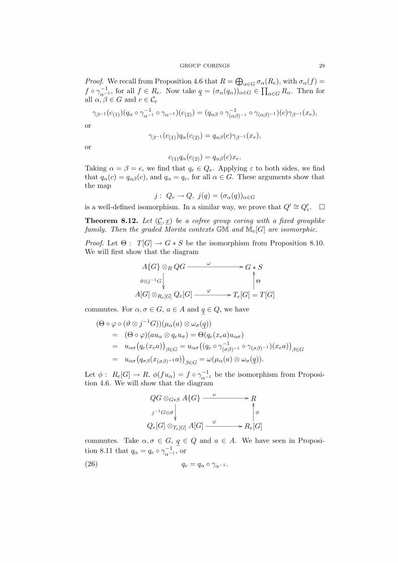
Theorem 8.12. Let (C, x) be a cofree group coring with a fixed grouplikefamily. Then the graded Morita contexts GM and Me[G] are isomorphic.

Proof. Let Θ : T [G] → G ∗ S be the isomorphism from Proposition 8.10.We will first show that the diagram

A{G} ⊗R QGω //

ϑ⊗j−1G��

G ∗ S

A[G]⊗Re[G] Qe[G]ϕ // Te[G] = T [G]

Θ

OO

commutes. For α, σ ∈ G, a ∈ A and q ∈ Q, we have

(Θ ◦ ϕ ◦ (ϑ⊗ j−1G))(µα(a)⊗ ωσ(q))

= (Θ ◦ ϕ)(auα ⊗ qeuσ) = Θ(qe(xea)uασ)

= uασ(qe(xea)

)β∈G = uασ

((qe ◦ γ−1

(σβ)−1 ◦ γ(σβ)−1)(xea))β∈G

= uασ(qσβ(x(σβ)−1a)

)β∈G = ω(µα(a)⊗ ωσ(q)).

Let φ : Re[G] → R, φ(fuα) = f ◦ γ−1α−1 be the isomorphism from Proposi-

tion 4.6. We will show that the diagram

QG⊗G∗S A{G}ν //

j−1G⊗ϑ��

R

Qe[G]⊗Te[G] A[G]ψ // Re[G]

φ

OO

commutes. Take α, σ ∈ G, q ∈ Q and a ∈ A. We have seen in Proposi-tion 8.11 that qα = qe ◦ γ−1

α−1 , or

(26) qe = qα ◦ γα−1 .


We have to show that

(φ ◦ ψ ◦ (j−1G⊗ ϑ))(ωσ(q)⊗ µα(a)) = (φ ◦ ψ)(qeuσ ⊗ auα)

= φ((qe · a)uσα) = qe · a ◦ γ−1(σα)−1

andν(ωσ(q)⊗ µα(a)) = qσα · a

are equal in Rσα = ∗C(σα)−1 . For γ(σα)−1(c) ∈ C(σα)−1 , we compute that

(qσα · a)(γ(σα)−1(c)) = (qσα ◦ γ(σα)−1)(c)a(26)= qe(c)a

= (qe · a)(c) = (qe · a ◦ γ−1(σα)−1)(γ(σα)−1(c)),

as needed. This finishes our proof. �

9. Galois group corings and graded Morita contexts

Let us call a G-A-coring C = (Cα)α∈G a left homogeneous progenerator ifevery Cα is a left A-progenerator. We will now apply the Morita theorydeveloped in the previous Section to find some equivalent properties for aleft homogeneous progenerator group coring to be Galois. Recall from [5]the following Theorem.

Theorem 9.1. Let (Ce, xe) be an A-coring with a fixed grouplike element,and assume that Ce is a left A-progenerator. We take a subring B of Te =AcoCe = {a ∈ A | axe = xea}, and consider the map

can′e : D′ = A⊗B A→ Ce, can′(a⊗B b) = axb.

Then the following statements are equivalent:(1) • can′e is an isomorphism of corings;

• A is faithfully flat as a left B-module.(2) • ∗can′e is an isomorphism of rings;

• A is a left B-progenerator.(3) • B = Te;

• the Morita context Me = (Te, Re, A,Qe, ϕe, ψe) is strict.(4) • B = Te;

• (F8, G8) is an equivalence of categories.

Here Me is the Morita context introduced in the light of Proposition 8.9,and (F8, G8) the adjoint pair of functors considered before Lemma 5.11. Inthe next Theorem we use the graded Morita context GM of Theorem 8.8,and the adjoint pair of functors (F7, G7) of Proposition 5.4.

Theorem 9.2. Let (C, x) be a left homogeneous progenerator G-A-coringwith a fixed grouplike family. We take a subring B of T = AcoC ⊂ Te, andconsider the map

can′ : D′ = (A⊗B A)〈G〉 → C, can′α(µα(a⊗B b)) = axαb.

Then the following statements are equivalent:(1) • can′ is an isomorphism of group corings;

GROUP CORINGS 31

• A is faithfully flat as a left B-module.(2) • ∗can′ is an isomorphism of graded rings;

• A is a left B-progenerator.(3) • B = T ∼= S;

• the graded Morita context GM = (G ∗ S,R,A{G}, QG, ω, ν) isstrict.

(4) • B = T ;• (F7, G7) is an equivalence of categories.

Proof. 1) ⇒ 2). Obviously ∗can′ is an isomorphism if can′ is an isomor-phism. In particular, can′e is an isomorphism of corings, hence it followsfrom Theorem 9.1 that A is a left B-progenerator.2) ⇒ 1). Suppose that ∗can′ : ∗C = R → ∗D′ = R′ is an isomorphism. Wethen have that the right dual (∗can′)∗ : R′∗ → R∗, (∗can′)∗(ϕ) = ϕ ◦ ∗can′

is also an isomorphism. Since C and D′ are left homogeneously finite, thismap can be interpreted as the isomorphism

f = ι−1 ◦ (∗can′)∗ ◦ ι′ :∏α∈G

D′α →

∏α∈G

Cα,

where we denoted respectively ι and ι′ for the isomorphisms∏α∈G Cα ∼= R∗

and∏α∈GD′

α∼= R′∗ (see the beginning of Section 4). For all d = (dα)α∈G ∈∏

α∈GD′α we have that

f(d) = (ι−1 ◦ (∗can′)∗ ◦ ι′)(d) = ι−1(ι′(d) ◦ ∗can′)

=((ι′(d) ◦ ∗can′)(f (α))c(α)

)α∈G =

(ι′(d)(f (α) ◦ can′α)c(α)

)α∈G

=(f (α)(can′α(dα))c(α)

)α∈G = (can′α(dα))α∈G,

i.e., f =∏α∈G can′α. Now, since f =

∏α∈G can′α is an isomorphism, it

follows that all can′α are isomorphisms. Indeed, (can′α)−1 = p′α ◦ f−1 ◦ iα :Cα → D′

α, where iα and p′α are the canonical injections and projections,respectively. So the inverse of can′ is given by (can′)−1 = ((can′α)−1)α∈G.Finally, since in particular ∗can′e is an isomorphism, Theorem 9.1 impliesthat A is faithfully flat as a left B-module.1) ⇒ 3). As in the proof of Proposition 5.10, C is a cofree group coring witha fixed grouplike family, since can′ : D′ → C is an isomorphism, and D′ iscofree. By Lemma 5.9 we then have that T = Te. Hence it follows fromTheorem 9.1 and the fact that can′e is an isomorphism that B = T and thatthe Morita context Me is strict. It is easily verified that the graded Moritacontext Me[G] then also is strict, and likewise GM, see Theorem 8.12. FromProposition 8.10 we get T ∼= S.4) ⇒ 1). By Proposition 5.7 can is an isomorphism, i.e. (C, x) is Galois.Hence (see Proposition 5.10) (C, x) is a cofree group coring with a fixedgrouplike familie, and thus Lemma 5.9 implies that B = T = Te. Since(F7

∼= F2 ◦F8, G7∼= G8 ◦G2) and (F2, G2) are equivalences (see Lemma 5.11


and Theorem 2.2), it follows that also (F8, G8) is an equivalence of cate-gories. Finally it follows from Theorem 9.1 that A is faithfully flat as a leftB-module.3) ⇒ 4). Suppose that GM = (G ∗ S,R,A{G}, QG, ω, ν) is a strict gradedMorita context. We then have a pair of inverse equivalences (F = − ⊗G∗SA{G}, G = −⊗R QG) between the categories MG

G∗S and MGR. By Proposi-

tion 8.10 we have that G ∗S and T [G] are isomorphic as graded rings. As aconsequence the categories MG

G∗S and MGT [G] are isomorphic, and the latter

is in turn isomorphic withMT by the Structure Theorem for graded modulesover strongly graded rings. Making use of the pair of functors (F3, G3) whichconstitutes an isomorphism between MG,C and MG

R (see Proposition 4.1),we have the following pair (F7, G7) of inverse equivalences between MT andMG,C :

F7 : MT∼= MG

T [G]∼= MG

G∗SeF // MG

ReGooG3 // MG,C : G7.F3

oo

For M ∈MT we have that

F7(M) =((M [G]⊗G∗S A{G}

)α

)α∈G

∈MG,C ,

where we denote(M [G]⊗G∗S A{G}

)α

for the αth homogeneous componentof M [G]⊗G∗S A{G} ∈ MG

R. The coaction maps of F7(M) are given by

ρα,β :(M [G]⊗G∗S A{G}

)αβ

→(M [G]⊗G∗S A{G}

)α⊗A Cβ ,

ρα,β

( ∑γ∈G

mγuγ ⊗G∗S µγ−1αβ(aγ))

=∑γ∈G

mγuγ ⊗G∗S µγ−1αβ(aγ) · f (β) ⊗A c(β)

=∑γ∈G

mγuγ ⊗G∗S µγ−1α(f (β)(xβaγ))⊗A c(β).

We now claim that F7∼= F7. For M ∈MT and α ∈ G, we consider the map

ϕM,α :(M [G]⊗G∗S A{G}

)α→ µα(M ⊗T A),

ϕM,α

( ∑γ∈G

mγuγ ⊗G∗S µγ−1α(aγ))

= µα

( ∑γ∈G

mγ ⊗T aγ).

ϕM,α is well-defined, since

ϕM,α

( ∑γ∈G

mγuγ · ueb⊗G∗S µγ−1α(aγ))

= ϕM,α

( ∑γ∈G

mγbeuγ ⊗G∗S µγ−1α(aγ))

= µα

( ∑γ∈G

mγbe ⊗T aγ)

GROUP CORINGS 33

equals

ϕM,α

( ∑γ∈G

mγuγ ⊗G∗S ueb · µγ−1α(aγ))

= ϕM,α

( ∑γ∈G

mγuγ ⊗G∗S µγ−1α(bγ−1αaγ))

= ϕM,α

( ∑γ∈G

mγuγ ⊗G∗S µγ−1α(beaγ))

= µα

( ∑γ∈G

mγ ⊗T beaγ),

for all b = i(be) ∈ S. Clearly ϕM,α is right A-linear. Let us check thatϕM = (ϕM,α)α∈G : F7(M) → F7(M) is a morphism in MG,C :

((ϕM,α ⊗A Cβ) ◦ ρα,β)( ∑γ∈G

mγuγ ⊗G∗S µγ−1αβ(aγ))

=∑γ∈G

ϕM,α

(mγuγ ⊗G∗S µγ−1α(f (β)(xβaγ))

)⊗A c(β)

=∑γ∈G

µα(mγ ⊗T f (β)(xβaγ))⊗A c(β)

=∑γ∈G

µα(mγ ⊗T 1A)f (β)(xβaγ)⊗A c(β)

=∑γ∈G

µα(mγ ⊗T 1A

)⊗A f (β)(xβaγ)c(β)

=∑γ∈G

µα(mγ ⊗T 1A

)⊗A xβaγ = ρα,β

(µαβ

( ∑γ∈G

mγ ⊗T aγ))

= (ρα,β ◦ ϕM,αβ)( ∑γ∈G

mγuγ ⊗G∗S µγ−1αβ(aγ)).

Let us finally show that ϕM is an isomorphism in MG,C . It suffices to checkthat the inverse of ϕM,α is given by

ϕ−1M,α

(µα

( n∑i=1

mi⊗T ai))

=n∑i=1

miue⊗G∗S µα(ai) =n∑i=1

miuα⊗G∗S µe(ai) :

(ϕ−1M,α ◦ ϕM,α)

( ∑γ∈G

mγuγ ⊗G∗S µγ−1α(aγ))

= ϕ−1M,α

(µα

( ∑γ∈G

mγ ⊗T aγ))

=∑γ∈G

mγue ⊗G∗S µα(aγ)

=∑γ∈G

mγue ⊗G∗S µγγ−1α(aγ) =∑γ∈G

mγue ⊗G∗S uγ1 · µγ−1α(aγ)

=∑γ∈G

mγue · uγ1⊗G∗S µγ−1α(aγ) =∑γ∈G

mγuγ ⊗G∗S µγ−1α(aγ);


(ϕM,α ◦ ϕ−1M,α)

(µα

( n∑i=1

mi ⊗T ai))

= ϕM,α

( n∑i=1

miue ⊗G∗S µα(ai))

=n∑i=1

µα(mi ⊗T ai) = µα

( n∑i=1

mi ⊗T ai).

So we have shown that F7 and F7 are naturally isomorphic. From theuniqueness of the adjoint functor, it follows that also G7

∼= G7. The factthat (F7, G7) is a pair of inverse equivalences implies that also (F7, G7) is apair of inverse equivalences, as needed. �

10. Application to H-comodule algebras

Let k be a commutative ring. Recall [15] that a Hopf G-coalgebra is a G-coalgebra H = (Hα)α∈G with the following additional structure: every Hα

is a k-algebra, such that ∆α,β and ε are algebra maps, and we have a familyof maps Sα : Hα−1 → Hα such that

Sα(h(1,α−1))h(2,α) = h(1,α)Sα(h(2,α−1)) = ε(h)1Hα ,

for every h ∈ He. A right G-H-comodule algebra is a k-algebra A with aright H-coaction ρ = (ρα)α∈G such that

ρα(ab) = a[0]b[0] ⊗ a[1,α]b[1,α] and ρα(1A) = 1A ⊗ 1Hα ,

for all a, b ∈ A and α ∈ G. This notion was introduced by the third authorin [17]. The proof of the following result is straightforward.

Proposition 10.1. Let H be a Hopf G-coalgebra, and A right G-H-comodulealgebra. Then C = A⊗H = (A⊗Hα)α∈G is a G-A-coring. The A-bimodulestructures are given by the formulas

a′(b⊗ h)a = a′ba[0] ⊗ ha[1,α],

for all a, a′, b ∈ A, α ∈ G, h ∈ Hα. The comultiplication and counit mapsare the following:

∆α,β : A⊗Hαβ → (A⊗Hα)⊗A(A⊗Hβ), ∆α,β(a⊗h) = (a⊗h(1,α))⊗A(1A⊗h(2,β));

ε = A⊗ ε : A⊗He → A.

x = (1A ⊗ 1Hα)α∈G is a grouplike family of A⊗H.

It is easy to see that, for a ∈ A, a ∈ AcoC if and only if a ⊗ 1Hα equals(1A ⊗ 1Hα)a = a[0] ⊗ a[1,α] = ρα(a), for all α ∈ G. With notation as in [20],this means that

AcoC = A0 = {a ∈ A | ρα(a) = a⊗ 1Hα , for all α ∈ G}.Let B → AcoC be a ring morphism. We can then compute the morphismcan : (A⊗B A)〈G〉 → A⊗H as follows: canα : µα(A⊗B A) → A⊗Hα isgiven by the formula

canα(µα(a⊗ b)) = a(1A ⊗ 1Hα)b = ab[0] ⊗ b[1,α].

GROUP CORINGS 35

This proves the following result.

Proposition 10.2. Let A be a right comodule algebra over a Hopf G-coalgebra H. Then (A ⊗H, (1A ⊗ 1Hα)α∈G) is a Galois G-A-coring if andonly if A is a G-H-Galois extension of AcoC = A0, in the sense of [20, Def.7.1].

Let H be a Hopf algebra, and H = (Hα)α∈G a set of isomorphic copies ofH, indexed by the group G. Let He = H, and λα : H → Hα the connectingisomorphism. Then H is a Hopf G-coalgebra, with structure maps

∆α,β(λαβ(h)) = λα(h(1))⊗ λβ(h(2));

Sα(λα−1(h)) = λα(S(h)).The counit is the counit of H, and every Hα is a k-algebra. We call H =H〈G〉 the cofree Hopf G-coalgebra associated to H. Using Propositions 5.10and 10.2, we obtain the following result:

Proposition 10.3. Let A be a right comodule algebra over a Hopf G-coalgebra H. A is a G-H-Galois extension of A0 if and only if H is acofree Hopf G-coalgebra and A is an H-Galois extension of AcoHe = A0.

A right relative (H,A)-Hopf module (in [20] termed a right G-(H,A)-Hopfmodule) is a right A-module M , with the additional structure of right H-comodule, such that the compatibility condition

ρα(ma) = m[0]a[0] ⊗m[1,α]a[1,α]

holds for all m ∈ M , a ∈ A, α ∈ G. MHA will denote the category of right

relative (H,A)-Hopf modules.In a similar way, a right relative group (H,A)-Hopf module is a family ofright A-modules (Mα)α∈G, with the additional structure (ρα,β)α,β∈G of rightG-H-comodule, with the compatibility relation

ραβ(ma) = m[0,α]a[0] ⊗m[1,α]a[1,β],

for all α, β ∈ G, m ∈ Mαβ and a ∈ A. The category of right relative group(H,A)-Hopf modules is denoted by MG,H

A . The proof of the following resultis straightforward, and is left to the reader.

Proposition 10.4. Let A be a right comodule algebra over a Hopf G-coalgebra H. Then we have isomorphisms of categories MH

A∼= MA⊗H and

MG,HA

∼= MG,A⊗H .

Let B → A0 be a ring morphism. It follows from Propositions 5.4 and 10.4that we have a pair of adjoint functors (F7, G7) between MB and MG,H

A . Asan application of Theorem 5.12, we obtain the following Structure Theoremfor relative group (H,A)-Hopf modules.

Proposition 10.5. Let A be a right comodule algebra over a Hopf G-coalgebra H, and B → A0 a ring morphism. Then the following assertionsare equivalent.


(1) B ∼= A0, A is a G-H-Galois extension of A0, and A is faithfully flatas a left B-module;

(2) (F7, G7) is a pair of inverse equivalences and A is flat as a left B-module.

Let us finally compute the left dual graded A-ring R of A⊗H. We have anisomorphism of k-modules

R =⊕α∈G

AHom(A⊗Hα−1 , A) ∼=⊕α∈G

Hom(Hα−1 , A).

The multiplication (and the A-bimodule structure) on R can be transportedto

⊕α∈G Hom(Hα−1 , A). We obtain the following multiplication rule, for

f ∈ Hom(Hα−1 , A) ∼= Rα, g ∈ Hom(Hβ−1 , A) ∼= Rβ, h ∈ H(αβ)−1 :

(27) (f#g)(h) = f(h(2,α−1))[0]g(h(1,β−1)f(h(2,α−1))[1,β−1]

).

Before we investigate more carefully the situation whereH is homogeneouslyfinite (that is, every Hα is a finitely generated and projective k-module, wemake some general observations.

Let K be a (classical) Hopf algebra, and A a left K-module algebra. Thenwe can form the smash product Kop#A, with multiplication rule

(28) (h#a)(k#b) = k(1)h#(k(2) · a)b.

It is well-known that Kop#A is an A-ring.We call K a graded Hopf algebra if K is a Hopf algebra and a G-gradedalgebra such that ∆(Kα) ⊂ Kα ⊗Kα and S(Kα) ⊂ Kα−1 . This implies inparticular that every Kα is a subcoalgebra of K. If K is a graded Hopfalgebra, and A is a left K-module algebra, then Kop#A is a graded A-ring.In [21], a G-graded Hopf algebra is called a Hopf G-algebra in packed form.The defining axioms of a Hopf G-algebra are formally dual to the definingaxioms of a Hopf G-coalgebra. A Hopf G-algebra is a family of k-coalgebrasK = (Kα)α∈G together with k-coalgebra maps µα,β : Kα ⊗Kβ → Kαβ andη : k → Ke satisfying the obvious associativity and unit properties. Wealso need antipode maps Sα : Kα → Kα−1 such that

µα−1,α(Sα(k(1))⊗ k(2)) = µα,α−1(k(1) ⊗ Sα(k(2))) = η(ε(k)),

for all k ∈ Kα. It is straightforward to show that K =⊕

α∈GKα is a gradedHopf algebra. Conversely, if K is a graded Hopf algebra, then (Kα)α∈G isa Hopf G-algebra. Thus we have an isomorphism between the categories ofG-graded Hopf algebras and Hopf G-algebras.If H is a homogeneously finite Hopf G-coalgebra, then K = (H∗

α−1)α∈G isa Hopf G-algebra, and, consequently, K =

⊕α∈GH

∗α−1 is a G-graded Hopf

algebra.If A is a right H-module algebra, then it is also a left K-module algebra,with action h∗ · a = 〈h∗, a[1,α−1]〉a[0], for all h∗ ∈ Kα = H∗

α−1 .

GROUP CORINGS 37

For every α ∈ G,

AHom(A⊗Hα−1 , A) ∼= Hom(Hα−1 , A) ∼= H∗α−1 ⊗A

is the degree α component of Kop#A.

Theorem 10.6. Let H be a homogeneously finite Hopf G-coalgebra, andA a right H-comodule algebra. Then R =

⊕α∈G AHom(A ⊗ Hα−1 , A) is

isomorphic to Kop#A as a G-graded A-ring. Consequently, the categoriesMG,C

A and MGKop#A are isomorphic.

Proof. We have to show that the k-module isomorphisms

λα : H∗α−1 ⊗A→ Hom(Hα−1 , A), λα(h∗ ⊗ a)(h) = 〈h∗, h〉a

transport the multiplication rule (28) to (27). Take α, β ∈ G, h∗ ∈ H∗α−1 ,

k∗ ∈ H∗β−1 , a, b ∈ A, and write f = λα(h∗ ⊗ a), g = λβ(k∗ ⊗ b). For

h ∈ H(αβ)−1 , we have

(f#g)(h) = 〈h∗, h(2,α−1)〉a[0]g(h(1,β−1)a[1,β−1])

= 〈h∗, h(2,α−1)〉〈k∗, h(1,β−1)a[1,β−1]〉a[0]b

= 〈h∗, h(2,α−1)〉〈k∗(1), h(1,β−1)〉〈k∗(2), a[1,β−1]〉a[0]b

= 〈k∗(1) ∗ h∗, h〉(k∗(2) · a)b

= λαβ(k∗(1) ∗ h∗#(k∗(2) · a)b)(h),

and we conclude that

λα(h∗ ⊗ a)#λβ(k∗ ⊗ b) = λαβ((h∗#a)(k∗#b)),

as needed. �

References

[1] H. Bass, Algebraic K-theory, Benjamin, New York, 1968.[2] P. Boisen, Graded Morita theory, J. Algebra 164 (1994), 1–25.[3] T. Brzezinski, The structure of corings. Induction functors, Maschke-type theorem,

and Frobenius and Galois properties, Algebr. Representat. Theory 5 (2002), 389–410.[4] T. Brzezinski and R. Wisbauer, “Corings and comodules”, London Math. Soc. Lect.

Note Ser. 309, Cambridge University Press, Cambridge, 2003.[5] S. Caenepeel, Galois corings from the descent theory point of view, Fields Inst. Comm

43 (2004), 163–186.[6] S. Caenepeel, M. De Lombaerde, A categorical approach to Turaev’s Hopf group

coalgebras, Comm. Algebra, 34 (2006), 2631–2657.[7] S. Caenepeel, T. Guedenon, Fully bounded noetherian rings and Frobenius extensions,

J. Algebra Appl., to appear.[8] S. Caenepeel, G. Militaru and Shenglin Zhu, “Frobenius and separable functors for

generalized module categories and nonlinear equations”, Lect. Notes in Math. 1787,Springer Verlag, Berlin, 2002.

[9] S. Caenepeel, F. Van Oystaeyen, “Brauer groups and the cohomology of gradedrings”, Monographs Textbooks Pure Appl. Math. 121, Marcel Dekker, New York,1988.

[10] S. Caenepeel, J. Vercruysse and Shuanhong Wang, Morita Theory for corings andcleft entwining structures, J. Algebra 276 (2004), 210–235.


[11] A. Marcus, Equivalences induced by graded bimodules, Comm. Algebra 26 (1998),713–731.

[12] C. Nastasescu, B. Torrecillas, “Graded coalgebras”, Tsukuba Math. J. 17 (1993),461–479.

[13] C. Nastasescu, F. Van Oystaeyen, “Methods of graded rings”, Lect. Notes in Math.1836, Springer Verlag, Berlin, 2004.

[14] M. E. Sweedler, The predual Theorem to the Jacobson-Bourbaki Theorem, Trans.Amer. Math. Soc. 213 (1975), 391–406.

[15] V.G. Turaev, Homotopy field theory in dimension 3 and crossed group-categories,preprint arXiv:math. GT/0005291.

[16] A. Virelizier, Hopf group-coalgebras, J. Pure Appl. Algebra 171 (2002), 75–122.[17] S. H. Wang, Group twisted smash products and Doi-Hopf modules for T -coalgebras,

Comm. Algebra 32 (2004), 3417–3436.[18] S. H. Wang, Group entwining structures and group coalgebra coextensions, Comm.

Algebra 32 (2004), 3437–3457.[19] S. H. Wang, A Maschke type theorem for Hopf π-comodules, Tsukuba J. Math. 28

(2004), 377–388.[20] S. H. Wang, Morita contexts, π-Galois extensions for Hopf π-coalgebras, Comm.

Algebra 34 (2006), 521–546.[21] M. Zunino, Double construction for crossed Hopf coalgebras, J. Algebra 278 (2004),

43–75.[22] M. Zunino, Yetter-Drinfeld modules for crossed structures, J. Pure Appl. Algebra

193 (2004), 313–343.

Faculty of Engineering, Vrije Universiteit Brussel, B-1050 Brussels, BelgiumE-mail address: [email protected]

URL: http://homepages.vub.ac.be/~scaenepe/

Faculty of Engineering, Vrije Universiteit Brussel, B-1050 Brussels, BelgiumE-mail address: [email protected]

URL: http://homepages.vub.ac.be/~krjansse/

Department of mathematics, Southeast University, Nanjing 210096, ChinaE-mail address: [email protected]

Documents

Introduction - Vrije Universiteit Brusselhomepages.vub.ac.be/~scaenepe/groupcorings7.pdf · We introduce group corings, ... in fact there is a categorical correspondence ... functors