Embed Size (px)
Citation preview

PROOF OF THE YANO-OBATA CONJECTURE FORHOLOMORPH-PROJECTIVE TRANSFORMATIONS
VLADIMIR S. MATVEEV AND STEFAN ROSEMANN
Abstract. We prove the classical Yano-Obata conjecture by showing that the connectedcomponent of the group of holomorph-projective transformations of a closed, connectedRiemannian Kahler manifold consists of isometries unless the metric has constant positiveholomorphic curvature.
1. Introduction
1.1. Definitions and main result. Let (M, g, J) be a Riemannian Kahler manifold ofreal dimension 2n ≥ 4. We denote by ∇ the Levi-Civita connection of g. All objects weconsider are assumed to be sufficiently smooth.
Definition 1. A regular curve γ : I → M is called h-planar, if there exist functionsα, β : I → R such that the ODE
(1) ∇γ(t)γ(t) = αγ(t) + βJ(γ(t))
holds for all t, where γ = ddtγ.
In certain papers, h-planar curves are called complex geodesics. The reason is that if weview the action of J on the tangent space as the multiplication with the imaginary uniti, the property of a curve γ to be h-planar means that ∇γ(t)γ(t) is proportional to γ(t)with a complex coefficient of the proportionality α(t) + i · β(t). Recall that geodesics (inan arbitrary, not necessary arc length parameter t) of a metric can be defined as curvessatisfying the equation ∇γ(t)γ(t) = α(t)γ(t).
Example 1. Consider the complex projective space
CP (n) = {1-dimensional complex subspaces of Cn+1}
with the standard complex structure J and the standard Fubini-Study metric gFS. Then,a regular curve γ is h-planar, if and only if it lies in a projective line.
Indeed, it is well known that every projective line L is a totally geodesic submanifoldof real dimension two such that its tangent space is invariant with respect to J . SinceL is totally geodesic, for every regular curve γ : I → L ⊆ CP (n) we have ∇γ(t)γ(t) ∈Tγ(t)L. Since L is two-dimensional, the vectors γ(t), J(γ(t)) form a basis in Tγ(t)L. Hence,∇γ(t)γ(t) = α(t)γ(t) + β(t)J(γ(t)) for certain α(t), β(t) as we claimed.
Institute of Mathematics, FSU Jena, 07737 Jena Germany,[email protected], [email protected].
partially supported by GK 1523 of DFG.1

2 VLADIMIR S. MATVEEV AND STEFAN ROSEMANN
Conversely, given a regular curve σ in CP (n) that satisfies equation (1) for some functionsα and β, we consider the projective line L such that σ(0) ∈ L and σ(0) ∈ Tσ(0)L. Solvingthe initial value problem γ(0) = σ(0) and γ(0) = σ(0) for ODE (1) with these functionsα and β on (L, gFS|L, J|L), we find a curve γ in L. Since L is totally geodesic, this curvesatisfies equation (1) on (CP (n), gFS, J). The uniqueness of a solution of an ODE impliesthat σ coincides with γ and, hence, is contained in L.
Definition 2. Let g and g be Riemannian metrics on M such that they are Kahler withrespect to the same complex structure J . They are called h-projectively equivalent, if everyh-planar curve of g is an h-planar curve of g and vice versa.
Remark 1. If two Kahler metrics g and g on (M,J) are affinely equivalent (i.e., if their Levi-Civita connections ∇ and ∇ coincide), then they are h-projectively equivalent. Indeed,the equation (1) for the first and for the second metric coincide if ∇ = ∇.
Definition 3. Let (M, g, J) be a Kahler manifold. A diffeomorphism f : M →M is calledan h-projective transformation, if f is holomorphic (that is, if f∗(J) = J), and if f ∗g ish-projectively equivalent to g. A vector field v is called h-projective, if its local flow Φv
t
consists of (local) h-projective transformations. Similarly, a diffeomorphism f : M → Mis called an affine transformation, if it preserves the Levi-Civita connection of g. A vectorfield v is affine, if its local flow consists of (local) affine transformations. An h-projectivetransformation (resp. h-projective vector field) is called essential, if it is not an affinetransformation (resp. affine vector field).
Clearly, the set of all h-projective transformations of (M, g, J) is a group. As it wasshown in [16] and [56], it is a finite-dimensional Lie group. We denote it by HProj(g, J). ByRemark 1, holomorphic affine transformations and holomorphic isometries are h-projectivetransformations, Iso(g, J) ⊆ Aff(g, J) ⊆ HProj(g, J). Obviously, the same is true for theconnected components of these groups containing the identity transformation: Iso0(g, J) ⊆Aff0(g, J) ⊆ HProj0(g, J).
Example 2 (Generalisation of the Beltrami construction from [3, 29]). Consider a non-degenerate complex linear transformation A ∈ Gln+1(C) and the induced bi-holomorphicdiffeomorphism fA : CP (n) → CP (n). Since the mapping fA sends projective lines toprojective lines, it sends h-planar curves (of the Fubiny-Study metric gFS) to h-planarcurves, see Example 1. Then, the pullback gA := f ∗
AgFS is h-projectively equivalent to gFS
and fA is an h-projective transformation. Note that the metric gA coincides with gFS (i.e.,fA is an isometry), if and only if A is proportional to a unitary matrix.
We see that for (CP (n), gFS, J) we have Iso0 6=HProj0. Our main result is
Theorem 1 (Yano-Obata conjecture). Let (M, g, J) be a closed, connected RiemannianKahler manifold of real dimension 2n ≥ 4. Then, Iso0(g, J) = HProj0(g, J) unless (M, g, J)can be covered by (CP (n), c · gFS, J) for some positive constant c.
Remark 2. The above Theorem is not true locally; one can construct counterexamples. Weconject that Theorem 1 is also true if we replace closedness by completeness; but dealing
PROOF OF THE YANO-OBATA CONJECTURE FOR h-PROJECTIVE TRANSFORMATIONS 3
with this case will require a lot of work. In particular, one will need to generalize theresults of [7] to the complete metrics.
1.2. History and motivation. h-projective equivalence was introduced by Otsuki andTashiro in [41, 49]. They have shown that the classical projective equivalence is not in-teresting in the Kahler situation since only simple examples are possible, and suggestedh-projective equivalence as an interesting object of study instead. This suggestion was veryfruitful. During 60th-70th, the theory of h-projectively equivalent metrics and h-projectivetransformations was one of the main research topics in Japanese and Soviet (mostly Odessaand Kazan) differential geometry schools, see for example the survey [37] with more thanone hundred fifty references. Two classical books [44, 54] contain chapters on h-projectivity.
The attribution of the Yano-Obato conjecture to Yano and Obata is in folklore - wedid not find a paper of them where they state this conjecture. It is clear though thatboth Obata and Yano (and many other geometers) tried to prove this statement and didthis under certain additional assumptions, see below. The conjectures of similar typewere standard in 60th-70th, in the time when Yano and Obata were active (and it wasalso, unfortunately, standard in that time not to publish conjectures or open questions).For example, another famous conjecture of that time states that an essential group ofconformal transformations of a Riemannian manifold is possible if and only if the manifoldis conformally equivalent to the standard sphere or to the Euclidean space; this conjectureis also attributed to Lichnerowicz and Obata though it seems that neither Lichnerowicznor Obata published it as a conjecture or a question; it was solved in Alekseevskii [2],Ferrand [8] and Schoen [43]. One more example is the so-called projective Lichnerowicz-Obata conjecture stating that a complete Riemannian manifold, such that the connectedcomponent of the neutral element of the projective group contains not only isometries,has constant positive sectional curvature. This conjecture was proved in [28, 27, 30, 34].Though this conjecture is also attributed in folklore to Lichnerowicz and Obata, neitherLichnerowicz nor Obata published this conjecture (however, this particular conjecture waspublished as “a classical conjecture” in [13, 38, 52]).
In view of these two examples, it would be natural to call the Yano-Obata conjecturethe Lichnerowicz-Obata conjecture for h-projective transformations.
Special cases of Theorem 1 were known before. For example, under the additionalassumption that the scalar curvature of g is constant, the conjecture was proven in [15, 55].The case when the Ricci tensor of g vanishes or is covariantly constant was proven earlierin [16, 17, 18]. Obata [39] and Tanno [48] proved this conjecture under the assumptionthat the h-projective vector field lies in the so-called k-nullity space of the curvature tensor.Many local results related to essential h-projective transformations are listed in the survey[37]. For example, in [35, 42] it was shown that locally symmetric spaces of non-constantholomorphic sectional curvature do not admit h-projective transformations, even locally.
Recent developments in the theory of h-projective equivalence are partially due to itsrelation to integrable systems, see [19, 20, 51]. In most cases, additional nondegeneracyconditions are assumed. These conditions imply that the manifold is a toric manifold andthe geodesic flow of its metric is completely integrable, see for example in [20] where strong

4 VLADIMIR S. MATVEEV AND STEFAN ROSEMANN
topological results were obtained. We will intensively use the relation to the integrablesystems in our paper, but we do not require any additional assumptions.
One more group of results that is very important for the present paper was obtainedin the recent paper [7]. In this paper, the Yano-Obata conjecture was proven under theassumption that the degree of mobility (see Definition 4) is ≥ 3. The methods of [7] camefrom the theory of overdetermined systems of finite type and are very different from themethods of the present paper.
2. The main equation of h-projective geometry and the scheme of theproof of Theorem 1
2.1. Main equation of h-projective geometry. Let g and g be two Riemannian (orpseudo-Riemannian) metrics on M2n≥4 that are Kahler with respect to the same complexstructure J . We consider the induced isomorphisms g : TM → T ∗M and g−1 : T ∗M →TM . Let us introduce the (1, 1)-tensor A(g, g) by the formula
(2) A(g, g) =
(det g
det g
) 12(n+1)
g−1 ◦ g : TM → TM
(in coordinates, the matrix of g−1 ◦ g is the product of the inverse matrix of g and thematrix of g).
Obviously, A(g, g) is non-degenerate, complex (in the sense that A ◦ J = J ◦ A) andself-adjoint with respect to both metrics. Let ∇ be the Levi-Civita connection of g.
Theorem 2 ([35]). The metric g is h-projectively equivalent to g, if and only if there existsa vector field Λ such that A = A(g, g) given by (2) satisfies
(3) (∇XA)Y = g(Y,X)Λ + g(Y,Λ)X + g(Y, JX)Λ + g(Y, Λ)JX,
for all x ∈M and all X,Y ∈ TxM , where Λ = J(Λ).
Remark 3. One may consider the equation (3) as a linear PDE-system on the unknown(A,Λ); the coefficients in this system depend on the metric g. Indeed, if the equation isfulfilled for X,Y being basis vectors, it is fulfilled for all vectors, see also the formula (4)below.
One can also consider equation (3) as a linear PDE-system on the (1, 1)-tensor A only,since the components of Λ can be obtained from the components of ∇A by linear algebraicmanipulations. Indeed, fix X and calculate the trace of the (1, 1)-tensors on the left andright-hand side of (3). The trace of the right-hand side equals 4g(Λ, X). Clearly, the traceof ∇XA is trace(∇XA) = X(traceA). Then, Λ = gradλ, where the function λ is equal to14traceA. In what follows, we prefer the last point of view and speak about a self-adjoint,
complex solution A of equation (3), instead of explicitly mentioning the pair (A,Λ).
Remark 4. Let g and g be two h-projectively equivalent Kahler metrics and A(g, g) thecorresponding solution of (3). It is easy to see that g and g are affinely equivalent, if andonly if the corresponding vector field Λ vanishes identically on M .
PROOF OF THE YANO-OBATA CONJECTURE FOR h-PROJECTIVE TRANSFORMATIONS 5
Remark 5. The original and more standard form of the equation (3) uses index (tensor)notation and reads
(4) aij,k = λigjk + λjgik − λiJjk − λjJik.
Here aij, λi and λi are related to A,Λ and Λ by the formulas aij = gipApj , λi = gipΛ
p and
λi = −gipΛp.
Remark 6. Note that formula (2) is invertible if A is non-degenerate: the metric g can bereconstructed from g and A by
(5) g = (det A)−12 g ◦ A−1
(we understand g as the mapping g : TM → T ∗M ; in coordinates, the matrix of g ◦ A−1
is the product of the matrices of g and A−1).Evidently, if A is g-self-adjoint and complex, g given by (5) is symmetric and invariant
with respect to the complex structure. It can be checked by direct calculations that if gis Kahler and if A is a non-degenerate, g-self-adjoint and complex (1, 1)-tensor satisfying(3), then g is also Kahler with respect to the same complex structure and is h-projectivelyequivalent to g.
Thus, the set of Kahler metrics, h-projectively equivalent to g, is essentially the sameas the set of self-adjoint, complex (in the sense J ◦ A = A ◦ J) solutions of (3) (the onlydifference is the case when A is degenerate, but since adding const ·Id to A does not changethe property of A to be a solution, this difference is not important).
By Remark 3, the equation (3) is a system of linear PDEs on the (1, 1)-tensor A.
Definition 4. We denote by Sol(g) the linear space of complex, self-adjoint solutions ofequation (3). The degree of mobility D(g) of a Kahler metric g is the dimension of thespace Sol(g).
Remark 7. We note that 1 ≤ D(g) <∞. Indeed, since Id is always a solution of equation(3), we have D(g) ≥ 1. We will not use the fact that D(g) <∞; a proof of this statementcan be found in [35].
Let us now show that the degree of mobility is the same for two h-projectively equivalentmetrics: we construct an explicit isomorphism.
Lemma 1. Let g and g be two h-projectively equivalent Kahler metrics on (M,J). Thenthe solution spaces Sol(g) and Sol(g) are isomorphic. The isomorphism is given by
A1 ∈ Sol(g) 7−→ A1 ◦ A(g, g)−1 ∈ Sol(g),
where A(g, g) is constructed by (2). In particular, D(g) is equal to D(g).
Proof. Let A = A(g, g) be the solution of (3) constucted by formula (2). If A1 ∈ Sol(g) is
non-degenerate, then g1 = (det A1)− 1
2 g ◦ A−11 is h-projectively equivalent to g by Remark
(6) and, hence, g1 is h-projectively equivalent to g. It follows that A2 = A(g, g1) ∈ Sol(g).On the other hand, using formula (2) we can easily verify that A2 = A1 ◦ A−1. If A1 isdegenerate, we can choose a real number t such that A1+tId is non-degenerate. As we have

6 VLADIMIR S. MATVEEV AND STEFAN ROSEMANN
already shown, (A1+tId)◦A−1 = A1◦A−1+tA−1 is contained in Sol(g). Since A−1 ∈ Sol(g),the same is true for A1 ◦A−1. We obtain that the mapping A1 7−→ A1 ◦A(g, g)−1 is a linearisomorphism between the spaces Sol(g) and Sol(g). �
Lemma 2 (Folklore). Let (M, g, J) be a Kahler manifold and let v be an h-projective vectorfield. Then the (1, 1)-tensor
(6) Av := g−1 ◦ Lvg −trace(g−1 ◦ Lvg)
2(n+ 1)Id
(where Lv is the Lie derivative with respect to v) is contained in Sol(g).
Proof. Since v is h-projective, gt = (Φvt )
∗g is h-projectively equivalent to g for every t. Itfollows that for every t the tensor At = A(g, gt) is a solution of equation (3). Since (3) islinear, Av :=
(ddtAt
)
|t=0is also a solution of (3) and it is clearly self-adjoint. Since the flow
of v preserves the complex structure, Av is complex. Using equation (2), we obtain thatAv is equal to
d
dt
[(det gt
det g
) 12(n+1)
g−1t ◦ g
]∣∣∣t=0
=1
2(n+ 1)
(d
dt
det gt
det g
∣∣∣t=0
)
Id +
(d
dtg−1
t ◦ g) ∣
∣∣t=0
=1
2(n+ 1)
(d
dt
det gt
det g
) ∣∣∣t=0
Id −(
g−1t ◦
(d
dtgt
)
◦ g−1t ◦ g
) ∣∣∣t=0
=1
2(n+ 1)
(d
dt
det gt
det g
) ∣∣∣t=0
Id + g−1 ◦ Lvg = −trace(g−1 ◦ Lvg)
2(n+ 1)+ g−1 ◦ Lvg.
Thus, Av ∈ Sol(g) as we claimed. �
2.2. Scheme of the proof of Theorem 1. If the degree of mobility D(g) ≥ 3, Theorem1 is an immediate consequence of [7, Theorem 1]. Indeed, by [7, Theorem 1], if D(g) ≥ 3and the manifold cannot be covered by (CP (n), c · gFS, J) for some c > 0, every metricg that is h-projectively equivalent to g is actually affinely equivalent to g. By [22], theconnected component of the neutral element of the group of affine transformations on aclosed manifold consists of isometries. Finally, we obtain HProj0 = Iso0.
If the degree of mobility is equal to one, every metric g that is h-projectively equivalentto g is proportional to g. Then, the group HProj0(g, J) acts by homotheties. Since themanifold is closed, it acts by isometries. Again, we obtain HProj0 = Iso0.
Thus, in the proof of Theorem 1, we may (and will) assume that the degree of mobilityof the metric g is equal to two.
The proof will be organized as follows. Sections 3 and 4 are technical. They are based ondifferent groups of methods and different ideas. In Section 3, we use the familiy of integralsfor the geodesic flow of the metric g found by Topalov [51]. With the help of these integrals,we prove that the eigenvalues of A behave quite regular, in particular we show that theyare globally ordered and that the multiplicity of every nonconstant eigenvalue is equal totwo. The assumptions of this section are global (in the sense that the metric is assumed tobe complete; actually, we only need that every two points can be connected by a geodesic).
PROOF OF THE YANO-OBATA CONJECTURE FOR h-PROJECTIVE TRANSFORMATIONS 7
In Section 4, we work locally with equation (3). We show that Λ and Λ from thisequation are commuting holomorphic vector fields that are nonzero at almost every point.We also deduce from (3) certain equations on the eigenvectors and eigenvalues of A: inparticular we show that the gradient of every eigenvalue is an eigenvector correspondingto this eigenvalue.
Beginning with Section 5, we require the assumption that the degree of mobility is equalto two. Moreover, we assume the existence of an h-projective vector field which is notalready an affine vector field. The main goal of Section 5 is to show that for every solutionA of equation (3) with the corresponding vector field Λ, in a neighborhood of almost everypoint there exists a function µ and a constant B < 0 (that can depend on the neighborhood)such that for all points x in this neighborhood and all X,Y ∈ TxM we have
(∇XA)Y = g(Y,X)Λ + g(Y,Λ)X + g(Y, JX)Λ + g(Y, Λ)JX
∇XΛ = µX +BA(X)
∇Xµ = 2Bg(X,Λ)
(7)
(one should view (7) as a PDE-system on (A,Λ, µ)).This is the longest and the most complicated part of the proof. First, in Section 5.1, we
combine Lemma 2 with the assumption that the degree of mobility is two to obtain theformulas (15,20) that describe the evolution of A along the flow of the h-projective vectorfield. With the help of the results of Section 4, we deduce (in the proof of Lemma 8) anODE for the eigenvalues of A along the trajectories of the h-projective vector field. ThisODE can be solved; combining the solutions with the global ordering of the eigenvaluesfrom Section 3, we obtain that A has at most three eigenvalues at every point; moreover,precisely one eigenvalue of A considered as a function on the manifold is not constant(unless the h-projective vector field is an affine vector field). As a consequence, in view ofthe results of Section 4, the vectors Λ and Λ are eigenvectors of A.
The equation (20) depends on two parameters. We prove that under the assumptionthat the manifold is closed, the parameters are subject of a certain algebraic equation sothat in fact the equation (20) depends on one parameter only. In order to do it, we workwith the distribution span{Λ, Λ} and show that its integral manifolds are totally geodesic.The equations (6,20) contain enough information to calculate the restriction of the metricto this distribution; the metric depends on the same parameters as the equation (20). Wecalculate the sectional curvature of this metric and see that it is unbounded (which can nothappen on a closed manifold), unless the parameters satisfy a certain algebraic equation.
In Section 5.3, we show that the algebraic conditions mentioned above imply the localexistence of B and µ such that (7) is fulfilled. This proves that the system (7) is satisfiedin a neighborhood of almost every point of M , for certain B, µ that can a priori dependon the neighborhood.
We complete the proof of Theorem 1 in Section 6. First we recall certain results of [7]to show that the constant B is the same in all neighborhoods implying that the system (7)is fulfilled on the whole manifold.
8 VLADIMIR S. MATVEEV AND STEFAN ROSEMANN
Once we have shown that the system (7) holds globally, Theorem 1 is an immediateconsequence of [48, Theorem 10.1].
2.3. Relation with projective equivalence and further directions of investigation.Two metrics g and g on the same manifold are projectively equivalent, if every geodesic ofg, after an appropriate reparametrization, is a geodesic of g. As we already mentionedabove, the notion “h-projective equivalence” appeared as an attempt to adapt the notion“projective equivalence” to Kahler metrics. It is therefore not a surprise that certain meth-ods from the theory of projectively equivalent metrics could be adapted to the h-projectivesituation. For example, the above mentioned papers [15, 55, 1] are actually h-projectiveanalogs of the papers [52, 14] (dealing with projective transformations), see also [11, 46].Moreover, [56, 49] are h-projective analogs of [18, 47], and many results listed in the survey[37] are h-projective analogs of those listed in [36].
The Yano-Obata conjecture is also an h-projective analog of the so-called projectiveLichnerowicz-Obata conjecture mentioned above and recently proved in [34, 30], see also [27,28]. The general scheme of our proof of the Yano-Obata conjecture is similar to the schemeof the proof of the projective Lichnerowicz-Obata conjecture in [34]. More precisely, as inthe projective case, the cases degree of mobility equal to two and degree of mobility ≥ 3were done using completely different groups of methods. As we mentioned above, theproof of the Yano-Obata conjecture for the metrics with degree of mobility ≥ 3 was donein [7]. This proof is based on other ideas than the corresponding part of the proofs of theprojective Lichnerowicz-Obata conjecture in [34, 32].
Concerning the proof under the assumption that the degree of mobility is two, the firstpart of the proof (Sections 3, 5.1) is based on the same ideas as in the projective case.More precisely, the way to use integrals for the geodesic flow to show the regular behaviorof the eigenvalues of A and their global ordering is very close to that of [4, 26, 31, 50].The way to obtain equation (20) that describes the evolution of A along the orbits of theh-projective vector field is close to that in [5] and is motivated by [27, 28, 30, 34].
The second part of the proof (Sections 4, 5.2) requires essentially new methods. Thereason is that the proof of the corresponding parts of the projective Lichnerowicz-Obataconjecture is based on the local description of projectively equivalent metrics due to Dini[6] and Levi-Civita [21]. This local description for h-projectively equivalent metrics is notknown yet; recent results of Kiyohara [19] suggest that it is expected to be much morecomplicated than in the projective case.
Concerning further perspective directions of investigation, one can try to obtain topo-logical obstructions that prevent a closed manifold to posses two h-projectively equivalentmetrics that are not affinely equivalent. In the projective case, the proof of certain topo-logical restrictions is based on the integrals for the geodesic flow, see [24, 25, 26, 29]; weexpect that these methods can be generalized for the h-projective case.
3. Quadratic integrals and the global ordering of the eigenvalues ofsolutions of equation (3)
PROOF OF THE YANO-OBATA CONJECTURE FOR h-PROJECTIVE TRANSFORMATIONS 9
3.1. Quadratic integrals for the geodesic flow of g. Let A be a self-adjoint, complexsolution of equation (3). By [51], for every t ∈ R, the function
Ft : TM → R , Ft(ζ) :=√
det (A− tId) g((A− tId)−1ζ, ζ)(8)
is an integral for the geodesic flow of g.
Remark 8. It is easy to prove (see formula (10) below) that the integrals are defined for allt ∈ R (i.e., even if A− tId is degenerate). Actually, the family Ft is a polynomial of degreen−1 in t whose coefficients are certain functions on TM ; these functions are automaticallyintegrals.
Remark 9. The integrals are visually close to the integrals for the geodesic flows of projec-tively equivalent metrics constructed in [23].
Later it will be useful to consider derivatives of the integrals defined above:
Lemma 3. Let {Ft} be the family of integrals given in equation (8). Then, for each integerm ≥ 0 and for each number t0 ∈ R,
(9)(
dm
dtmFt
)
|t=t0
is also an integral for the geodesic flow of g.
Proof. As we already mentioned above in Remark 8,
Ft(ζ) = sn−1(ζ)tn−1 + ...+ s1(ζ)t+ s0(ζ)
for certain integrals s0, ..., sn−1 : TM → R. Then, the t-derivatives (9) are also polynomialsin t whose coefficients are integrals, i.e., the t-derivatives (9) are also integrals for everyfixed t0. �
3.2. Global ordering of the eigenvalues of solutions of equation (3). During thewhole subsection let A be an element of Sol(g); that is, A is a complex, self-adjoint (1, 1)-tensor such that it is a solution of equation (3). Since it is self-adjoint with respect to (apositively-definite metric) g, the eigenvalues of A|x := A|TxM are real.
Definition 5. We denote by m(y) the number of different eigenvalues of A at the point y.Since A ◦ J = J ◦ A, each eigenvalue has even multiplicity ≥ 2. Hence, m(y) ≤ n for ally ∈M . We say that x ∈M is a typical point for A if m(x) = maxy∈M{m(y)}. The set ofall typical points of A will be denoted by M0 ⊆M .
Let us denote by µ1(x) ≤ ... ≤ µn(x) the eigenvalues of A counted with half of theirmultiplicities. The functions µ1, ..., µn are real since A is self-adjoint and they are at leastcontinuous. It follows that M0 ⊆ M is an open subset. The next theorem shows thatM0 is dense in M (we prove this theorem under the assumption that M is complete andconnected; actually, we only need that every two points can be connected by a geodesic).
Theorem 3. Let (M, g, J) be a complete, connected Riemannian Kahler manifold of realdimension 2n. Then, for every A ∈ Sol(g) and every i = 1, ..., n − 1, the following state-ments hold:
10 VLADIMIR S. MATVEEV AND STEFAN ROSEMANN
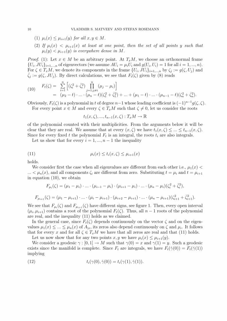
(1) µi(x) ≤ µi+1(y) for all x, y ∈M .
(2) If µi(x) < µi+1(x) at least at one point, then the set of all points y such thatµi(y) < µi+1(y) is everywhere dense in M .
Proof. (1): Let x ∈ M be an arbitrary point. At TxM , we choose an orthonormal frame{Ui, JUi}i=1,...,n of eigenvectors (we assume AUi = µiUi and g(Ui, Ui) = 1 for all i = 1, ..., n).For ζ ∈ TxM , we denote its components in the frame {Ui, JUi}i=1,...,n by ζj := g(ζ, Uj) andζj := g(ζ, JUj). By direct calculations, we see that Ft(ζ) given by (8) reads
(10)Ft(ζ) =
n∑
i=1
[
(ζ2i + ζ2
i )n∏
j=1;j 6=i
(µj − µi)]
= (µ2 − t) · ... · (µn − t)(ζ21 + ζ2
1 ) + ...+ (µ1 − t) · ... · (µn−1 − t)(ζ2n + ζ2
n).
Obviously, Ft(ζ) is a polynomial in t of degree n−1 whose leading coefficient is (−1)n−1g(ζ, ζ).For every point x ∈M and every ζ ∈ TxM such that ζ 6= 0, let us consider the roots
t1(x, ζ), ..., tn−1(x, ζ) : TxM → R
of the polynomial counted with their multiplicities. From the arguments below it will beclear that they are real. We assume that at every (x, ζ) we have t1(x, ζ) ≤ ... ≤ tn−1(x, ζ).Since for every fixed t the polynomial Ft is an integral, the roots ti are also integrals.
Let us show that for every i = 1, ..., n− 1 the inequality
(11) µi(x) ≤ ti(x, ζ) ≤ µi+1(x)
holds.We consider first the case when all eigenvalues are different from each other i.e., µ1(x) <
... < µn(x), and all components ζi are different from zero. Substituting t = µi and t = µi+1
in equation (10), we obtain
Fµi(ζ) = (µ1 − µi) · ... · (µi−1 − µi) · (µi+1 − µi) · ... · (µn − µi)(ζ
2i + ζ2
i ),
Fµi+1(ζ) = (µ1 − µi+1) · ... · (µi − µi+1) · (µi+2 − µi+1) · ... · (µn − µi+1)(ζ
2i+1 + ζ2
i+1).
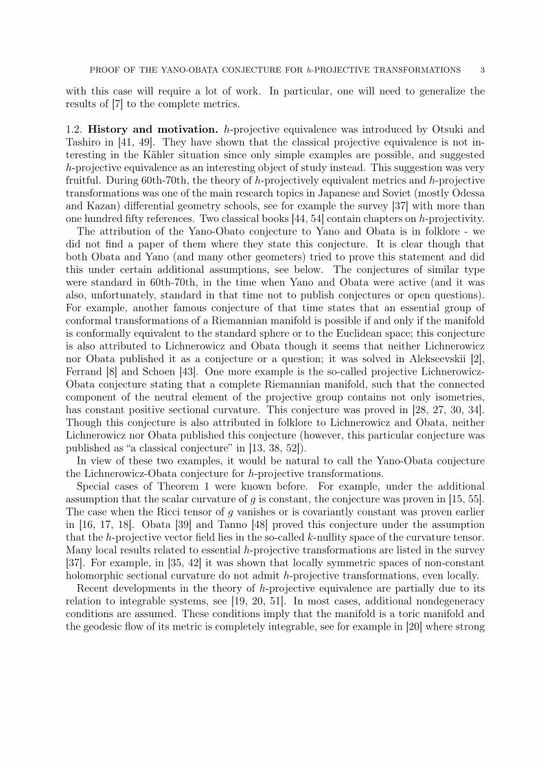
We see that Fµi(ζ) and Fµi+1
(ζ) have different signs, see figure 1. Then, every open interval(µi, µi+1) contains a root of the polynomial Ft(ζ). Thus, all n− 1 roots of the polynomialare real, and the inequality (11) holds as we claimed.
In the general case, since Ft(ζ) depends continuously on the vector ζ and on the eigen-values µ1(x) ≤ ... ≤ µn(x) of A|x, its zeros also depend continuously on ζ and µi. It followsthat for every x and for all ζ ∈ TxM we have that all zeros are real and that (11) holds.
Let us now show that for any two points x, y we have µi(x) ≤ µi+1(y).We consider a geodesic γ : [0, 1] →M such that γ(0) = x and γ(1) = y. Such a geodesic
exists since the manifold is complete. Since Ft are integrals, we have Ft(γ(0)) = Ft(γ(1))implying
(12) ti(γ(0), γ(0)) = ti(γ(1), γ(1)).
PROOF OF THE YANO-OBATA CONJECTURE FOR h-PROJECTIVE TRANSFORMATIONS 11
µi−1
µi
µi+1
Ft(ζ, ζ)
tti−1 ti
Figure 1. If µ1 < µ2 < ... < µn and all ζi 6= 0, the values of Ft(ζ) havedifferent signs at t = µi and t = µi+1 implying the existence of a root ti suchthat µi < ti < µi+1.
y
U
µi = µi+1
x
µi(x) < µi+1(x)
ζ
γζ(t)
Figure 2. The initial velocity vectors ζ at x of the geodesics connectingthe point x with points from U form a subset of nonzero measure and arecontained in Uµ.
Combining (11) and (12), we obtain
µi(x)(11)
≤ ti(x, γ(0))(12)= ti(y, γ(1))
(11)
≤ µi+1(y)
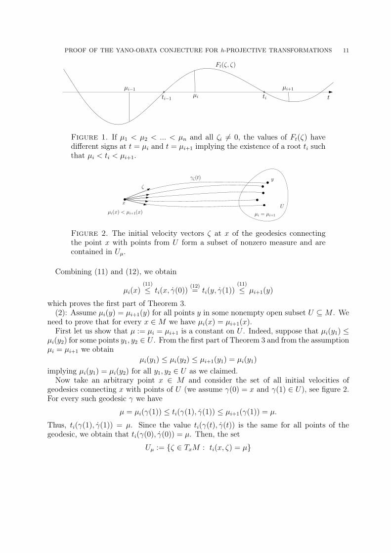
which proves the first part of Theorem 3.(2): Assume µi(y) = µi+1(y) for all points y in some nonempty open subset U ⊆M . We
need to prove that for every x ∈M we have µi(x) = µi+1(x).First let us show that µ := µi = µi+1 is a constant on U . Indeed, suppose that µi(y1) ≤
µi(y2) for some points y1, y2 ∈ U . From the first part of Theorem 3 and from the assumptionµi = µi+1 we obtain
µi(y1) ≤ µi(y2) ≤ µi+1(y1) = µi(y1)
implying µi(y1) = µi(y2) for all y1, y2 ∈ U as we claimed.Now take an arbitrary point x ∈ M and consider the set of all initial velocities of
geodesics connecting x with points of U (we assume γ(0) = x and γ(1) ∈ U), see figure 2.For every such geodesic γ we have
µ = µi(γ(1)) ≤ ti(γ(1), γ(1)) ≤ µi+1(γ(1)) = µ.
Thus, ti(γ(1), γ(1)) = µ. Since the value ti(γ(t), γ(t)) is the same for all points of thegeodesic, we obtain that ti(γ(0), γ(0)) = µ. Then, the set
Uµ := {ζ ∈ TxM : ti(x, ζ) = µ}
12 VLADIMIR S. MATVEEV AND STEFAN ROSEMANN
has nonzero measure. Since Uµ is contained in the set
{ζ ∈ TxM : Fµ(ζ) = 0}which is a quadric in TxM , the latter must coincide with the whole TxM . In view offormula (10), this implies that at least two eigenvalues of A at x should be equal to µ.Suppose the multiplicity of the eigenvalue µ is equal to 2k. This implies that µr+1(x) =... = µr+k(x) = µ, µr(x) 6= µ and µr+k+1(x) 6= µ. If i ∈ {r + 1, ..., r + k − 1}, we are done.We assume that i 6∈ {r + 1, ..., r + k − 1} and find a contradiction.
In order to do it, we consider the function
F : R × TM → R , Ft(ζ) := Ft(ζ)/(t− µ)k−1.
At the point x, each term of the sum (10) contains (t − µ)k−1 implying that Ft(ζ) is apolynomial in t (and is a quadratic function in ζ). Since for every fixed t0 the function Ft0
is an integral, the function Ft0 is also an integral. Let us show that for every geodesic γ
with γ(0) = x and γ(1) ∈ U we have that(
Ft(γ(0)))
|t=µ= 0. Indeed, we already have
shown that ti(x, γ(0)) = µ. By similar arguments, in view of inequality (11), we obtaintr+1(x, γ(0)) = ... = tr+k−1(x, γ(0)) = µ. Then, t = µ is a root of multiplicity k of Ft(γ(0))and, therefore, a root of multiplicity k − (k − 1) = 1 of Ft(γ(0)) = Ft(γ(0))/(t − µ)k−1.Finally, Fµ(γ(0)) = 0.
Now, in view of the formula (10), the set {ζ ∈ TxM : Fµ(ζ) = 0} is a nontrivial (sinceµr 6= µ 6= µr+k+1) quadric in TxM , which contradicts the assumption that it containsa subset Uµ of nonzero measure. Finally, we have i, i + 1 ∈ {r + 1, ..., r + k} implyingµi(x) = µi+1(x) = µ. �
From Theorem 3, we immediately obtain the following two corollaries:
Corollary 1. Let (M, g, J) be a complete, connected Riemannian Kahler manifold. Then,for every A ∈ Sol(g), the set M0 of typical points of A is open and dense in M .
Corollary 2. Let (M, g, J) be a complete, connected Riemannian Kahler manifold and as-sume A ∈ Sol(g). Then, at almost every point the multiplicity of a non-constant eigenvalueρ of A is equal to two.
4. Basic properties of solutions A of equation (3)
4.1. The vector fields Λ and Λ are holomorphic.
Lemma 4 (Corollary 3 from [7]). Let (M, g, J) be a Kahler manifold of real dimension2n ≥ 4 and let be A ∈ Sol(g). Let Λ be the corresponding vector field defined by equation(3). Then Λ is a Killing vector field for the Kahler metric g i.e.,
g(∇XΛ, Y ) + g(X,∇Y Λ) = 0
for all X,Y ∈ TM .

PROOF OF THE YANO-OBATA CONJECTURE FOR h-PROJECTIVE TRANSFORMATIONS 13
It is a well-known fact that if a Killing vector field K vanishes on some open nonemptysubset U of the connected manifold M , then K vanishes on the whole M . From this, weconclude
Corollary 3. Let (M, g, J) be a connected Kahler manifold of real dimension 2n ≥ 4 andlet v be an h-projective vector field.
(1) If v restricted to some open nonempty subset U ⊆M is a Killing vector field, thenv is a Killing vector field on the whole M .
(2) If v is not identically zero, the set of points Mv 6=0 := {x ∈ M : v(x) 6= 0} is openand dense in M .
Proof. (1) Suppose the restriction of v to an open subset U is a Killing vector field. Then,gt = (Φv
t )∗g restricted to U ′ ⊂ U is equal to g|U ′ for sufficiently small t. Hence, At|U ′ =
A(g, gt)|U ′ = Id. The corresponding vector field Λt = 14grad traceAt vanishes (on U ′)
implying Λt vanishes (on U ′) as well. Since Λt is a Killing vector field, Λt vanishes on thewhole manifold implying Λt is equal to zero on the whole M . Then, by (3), the (1, 1)-tensorAt−Id is covariantly constant on the whole M . Since this tensor vanishes on U ′, it vanisheson the whole manifold. Finally, At = Id on M , implying that v is a Killing vector field onM . This proves part (1) of Corollary 3.
(2) Suppose v vanishes on some open subset U ⊆ M . To prove (2), we have to showthat v = 0 everywhere on M . From part (1) we can conclude that v is a Killing vectorfield on M . Since v vanishes on (open, nonempty) U , it vanishes on the whole M . �
The next lemma combined with Lemma 4 shows that Λ is a holomorphic vector field.
Lemma 5. Let (M, g, J) be a Kahler manifold. Let K be a vector field of the form K =Jgrad f for some function f . Then K is a Killing vector field for g, if and only if K isholomorphic.
Proof. The statement of the lemma follows from the straight-forward calculation below,where we use that ∇J = 0 and that ∇grad f is a self-adjoint (1, 1)-tensor. We obtain
g(Y, (LKJ)X) = g(Y, J∇XK) − g(Y,∇JXK) = −g(Y,∇Xgrad f) − g(Y,∇JXK)
= −g(X,∇Y grad f) − g(Y,∇JXK) = −g(JX,∇YK) − g(∇JXK,Y )
for arbitrary vectors X and Y . It follows that LKJ = 0, if and only if K satisfies theKilling equation as we claimed. �
Corollary 4. Let (M, g, J) be a Kahler manifold of real dimension 2n ≥ 4. Then, forevery A ∈ Sol(g) the vector fields Λ and Λ from (3) are holomorphic and commuting, i.e.,
LΛJ = LΛJ = 0 and [Λ, Λ] = 0.
Proof. By Remark 3, Λ is the gradient of a function. Since Λ = JΛ is a Killing vector field,by Lemma 5 we have that Λ is holomorphic. Since the multiplication with the complexstructure sends holomorphic vector fields to holomorphic vector fields, Λ is holomorphic aswell. By direct calculations, [Λ, Λ] = (LΛJ)Λ + J [Λ,Λ] = 0. �

14 VLADIMIR S. MATVEEV AND STEFAN ROSEMANN
4.2. Covariant derivatives of the eigenvectors of A. Let A be a complex, self-adjointsolution of equation (3). On M0, the eigenspace distributions EA(µi) are well-definedand differentiable. In general, they are not integrable (except for the trivial case whenthe metrics are affinely equivalent). The next proposition explains the behavior of thesedistributions.
Proposition 1. Let (M, g, J) be a Riemannian Kahler manifold and assume A ∈ Sol(g).Let U be a smooth field of eigenvectors of A defined on some open subset of M0. Let ρ bethe corresponding eigenvalue. Then, for an arbitrary vector X ∈ TM , we have
(A− ρId)∇XU = X(ρ)U − g(U,X)Λ − g(U,Λ)X − g(U, JX)Λ − g(U, Λ)JX.(13)
Moreover, if V is an eigenvector of A corresponding to an eigenvalue τ 6= ρ, then V (ρ) = 0and grad ρ ∈ EA(ρ).
Proof. Using equation (3), we obtain
(∇XA)U = g(U,X)Λ + g(U,Λ)X + g(U, JX)Λ + g(U, Λ)JX
for arbitrary X ∈ TM . On the other hand, since U ∈ EA(ρ), we calculate
∇X(AU) = ∇X(ρU) = X(ρ)U + ρ∇XU.
Inserting the last two equations in ∇X(AU) = (∇XA)U + A(∇XU), we obtain (13).Now let τ be another eigenvalue of A, such that ρ 6= τ , and let V ∈ EA(τ). Replacing Vwith X in equation (13) and using that EA(ρ) ⊥ EA(τ), we obtain
(A− ρId)∇VU = V (ρ)U − g(U,Λ)V − g(U, Λ)JV.
Since the left-hand side of the equation above is orthogonal to EA(ρ), we immediately ob-tain 0 = V (ρ) = g(V, grad ρ). Thus, grad ρ is orthogonal to all eigenvectors correspondingto eigenvalues different from ρ implying it lies in EA(ρ) as we claimed. �
5. Kahler manifolds of degree of mobility D(g) = 2 admitting essentialh-projective vector fields
For closed manifolds, the condition HProj0 6= Iso0 is equivalent to the existence of anessential (i.e., not affine) h-projective vector field. The goal of this section is to prove thefollowing
Theorem 4. Let (M, g, J) be a closed, connected Riemannian Kahler manifold of realdimension 2n ≥ 4 and of degree of mobility D(g) = 2 admitting an essential h-projectivevector field. Let A ∈ Sol(g) with the corresponding vector field Λ.
Then, almost every point y ∈M has a neighborhood U(y) such that there exists a constantB < 0 and a smooth function µ : U(y) → R such that the system
(∇XA)Y = g(Y,X)Λ + g(Y,Λ)X + g(Y, JX)Λ + g(Y, Λ)JX
∇XΛ = µX +BA(X)
∇Xµ = 2Bg(X,Λ)
(14)
is satisfied for all x in U(y) and all X,Y ∈ TxU .

PROOF OF THE YANO-OBATA CONJECTURE FOR h-PROJECTIVE TRANSFORMATIONS 15
One should understand (14) as the system of PDEs on the components of (A,Λ, µ).Actually, in the system (14), the first equation is the equation (3) and is fulfilled by thedefinition of Sol(g), so our goal is to prove the local existence of B and µ such that thesecond and the third equation of (14) are fulfilled.
Remark 10. If D(g) ≥ 3, the conclusion of this theorem is still true if we allow all, i.e.,not necessary negative, values of B. In this case we even do not need the ‘closedness’assumptions (i.e., the statement is local) and the existence of an h-projective vector field,see [7]. Theorem 4 essentially needs the existence of an h-projective vector field and is nottrue locally.
5.1. The tensor A has at most two constant and precisely one non-constanteigenvalue. First let us prove
Lemma 6. Let (M, g, J) be a Kahler manifold of real dimension 2n ≥ 4 and of degree ofmobility D(g) = 2. Suppose f : M →M is an h-projective transformation for g and let Abe an element of Sol(g). Then f maps the set M0 of typical points of A onto M0.
Proof. Let x be a point of M0. Since the characteristic polynomial of (f ∗A)|x is the sameas for A|f(x), we have to show that the number of different eigenvalues of (f ∗A)|x and A|xcoincide. If A is proportional to the identity on TM , the assertion follows immediately.Let us therefore assume that {A, Id} is a basis for Sol(g). We can find neighborhoods Ux
and f(Ux) of x and f(x) respectively, such that A is non-degenerate in these neighborhoods
(otherwise we add t · Id to A with a sufficiently large t ∈ R+). By (5), g = (det A)−12 g ◦
A−1, g, f ∗g and f ∗g are h-projectively equivalent to each other in Ux. By direct calculation,we see that f ∗A = f ∗A(g, g) = A(f ∗g, f ∗g). Hence, f ∗A is contained in Sol(f ∗g). Firstsuppose that A(g, f ∗g) is proportional to the identity. We obtain that
f ∗A = αA+ βId
for some constants α, β. Since α 6= 0 (if A is non-proportional to Id, the same holds forf ∗A), the number of different eigenvalues of (f ∗A)|x is the same as for A|x. It follows thatf(x) ∈ M0. Now suppose that A(g, f ∗g) is non-proportional to Id. Then, the numbersof different eigenvalues for A|x and A(g, f ∗g)|x coincide. By Lemma 1, D(f ∗g) = 2 and{A(g, f ∗g)−1, Id} is a basis for Sol(f ∗g). We obtain that
f ∗A = γA(g, f ∗g)−1 + δId
for some constants γ 6= 0 and δ. It follows that the numbers of different eigenvalues of(f ∗A)|x and A(g, f ∗g)−1
|x coincide. Thus, the number of different eigenvalues of (f ∗A)|x is
equal to the number of different eigenvalues of A|x. Again we have that f(x) ∈ M0 as weclaimed. �
Convention. In what follows, (M, g, J) is a closed, connected Riemannian Kahler man-ifold of real dimension 2n ≥ 4 and of degree of mobility D(g) = 2. We assume that v isan h-projective vector field which is not affine. We chose a real number t0 such that thepullback g := (Φv
t0)∗g is not affinely equivalent to g. Let A = A(g, g) be the corresponding
element in Sol(g) constructed by formula (2).
16 VLADIMIR S. MATVEEV AND STEFAN ROSEMANN
Lemma 7. The tensor A and the h-projective vector field v satisfy
LvA = c2A2 + c1A+ c0Id(15)
for some constants c2 6= 0, c1, c0.
Proof. Note that the vector field v is also h-projective with respect to the metric g andthe degrees of mobility of the metrics g and g are both equal to two (see Lemma 1). SinceA = A(g, g) is not proportional to the identity and A(g, g) = A(g, g)−1 ∈ Sol(g), we obtainthat {A, Id} and {A−1, Id} form bases for Sol(g) and Sol(g) respectively. It follows fromLemma 2 that
g−1 ◦ Lvg − trace(g−1◦Lvg)2(n+1)
Id = β1A+ β2Id,
g−1 ◦ Lvg − trace(g−1◦Lv g)2(n+1)
Id = β3A−1 + β4Id
(16)
for some constants β1, β2, β3 and β4. Taking the trace on both sides of the above equations,we see that they are equivalent to
g−1 ◦ Lvg = β1A+(
12β1 traceA+ (n+ 1)β2
)Id,
g−1 ◦ Lvg = β3A−1 +
(12β3 traceA−1 + (n+ 1)β4
)Id.
(17)
By (5), g can be written as g = (det A)−12 g ◦ A−1. Then,
g−1 ◦ Lvg(5)= (det A)
12A ◦ g−1 ◦ Lv((det A)−
12 g ◦ A−1)
= −1
2(det A)−1(Lv det A)Id + A ◦ (g−1 ◦ Lvg) ◦ A−1 − (LvA) ◦ A−1.
We insert the second equation of (17) in the left-hand side, the first equation of (17) inthe right-hand side and multiply with A from the right to obtain
β3Id +(
12β3 traceA−1 + (n+ 1)β4
)A
= −12(det A)−1(Lv det A)A+ β1A
2 +(
12β1 traceA+ (n+ 1)β2
)A− LvA.
Rearranging the terms in the last equation, we obtain
LvA = c2A2 + c1A+ c0Id(18)
for constants c2 = β1, c0 = −β3, and a certain function c1.
Remark 11. Our way to obtain the equation (18) is based on an idea of Fubini from [9]used in the theory of projective vector fields.
Our next goal is to show that c2 = β1 6= 0. If β1 = 0, the first equation of (17) reads
Lvg = (n+ 1)βg
hence, v is an infinitesimal homothety for g. This contradicts the assumption that v isessential and we obtain that c2 = β1 6= 0.Now let us show that the function c1 is a constant. Since A is nondegenerate, c1 is a smoothfunction, so it is sufficient to show that its differential vanishes at every point of M0. Wewill work in a neighborhood of a point of M0. Let U ∈ EA(ρ) be an eigenvector of A with
PROOF OF THE YANO-OBATA CONJECTURE FOR h-PROJECTIVE TRANSFORMATIONS 17
corresponding eigenvalue ρ. Using the Leibniz rule for the Lie derivative and the conditionthat U ∈ EA(ρ), we obtain the equations
Lv(AU) = Lv(ρU) = v(ρ)U + ρ[v, U ] and Lv(AU) = (LvA)U + A([v, U ]).
Combining both equations and inserting LvA from (18), we obtain
(v(ρ) − c2ρ2 − c1ρ− c0)U = (A− ρId)[v, U ].
In a basis of eigenvectors {Ui, JUi} of A from the proof of Theorem 3, we see that theright-hand side does not contain any component from EA(ρ) (i.e., the right-hand side is alinear combination of eigenvectors corresponding to other eigenvalues). Then,
c1 = v(ln(ρ)) − c2ρ−c0ρ
and (A− ρId)[v, U ] = 0.(19)
These equations are true for all eigenvalues ρ of A and corresponding eigenvectors U .Note that ρ 6= 0 since A is non-degenerate. By construction, the metric g (such thatA = A(g, g)) is not affinely equivalent to g, in particular, A has more than one eigenvalue.Let be W ∈ EA(µ) and ρ 6= µ. Applying W to the first equation in (19) and usingProposition 1, we obtain
W (c1) = [W, v](ln(ρ)).
The second equation of (19) shows that [v,W ] = 0 modulo EA(µ). Hence,
W (c1) = 0.
We obtain that U(c1) = 0 for all eigenvectors U of A. Then, dc1 ≡ 0 on M0. Since M0
is dense in M , we obtain that dc1 ≡ 0 on the whole M implying c1 is a constant. Thiscompletes the proof of Lemma 7. �
Convention. Since c2 6= 0, we can replace v by the h-projective vector field 1c2v. For
simplicity, we denote the new vector field again by v; this implies that equation (15) is nowsatisfied for c2 = 1: instead of (15) we have
LvA = A2 + c1A+ c0Id(20)
for some constants c1, c0.
Remark 12. Note that the constant β1 in the proof of Lemma 7 is equal to c2. With theconvention above, the first equation in (16) now reads
Av = g−1 ◦ Lvg −trace(g−1 ◦ Lvg)
2(n+ 1)Id = A+ βId(21)
for some β ∈ R.
Lemma 8. The tensor A has precisely one non-constant eigenvalue ρ of multiplicity 2and at least one and at most two constant eigenvalues (we denote the constant eigenvaluesby ρ1 < ρ2 and their multiplicities by 2k1 and 2k2 = 2n − 2k1 − 2 respectively; we allowk1 to be equal to 0 and n − 1; if k1 = 0, A has only one constant eigenvalue ρ2 and if
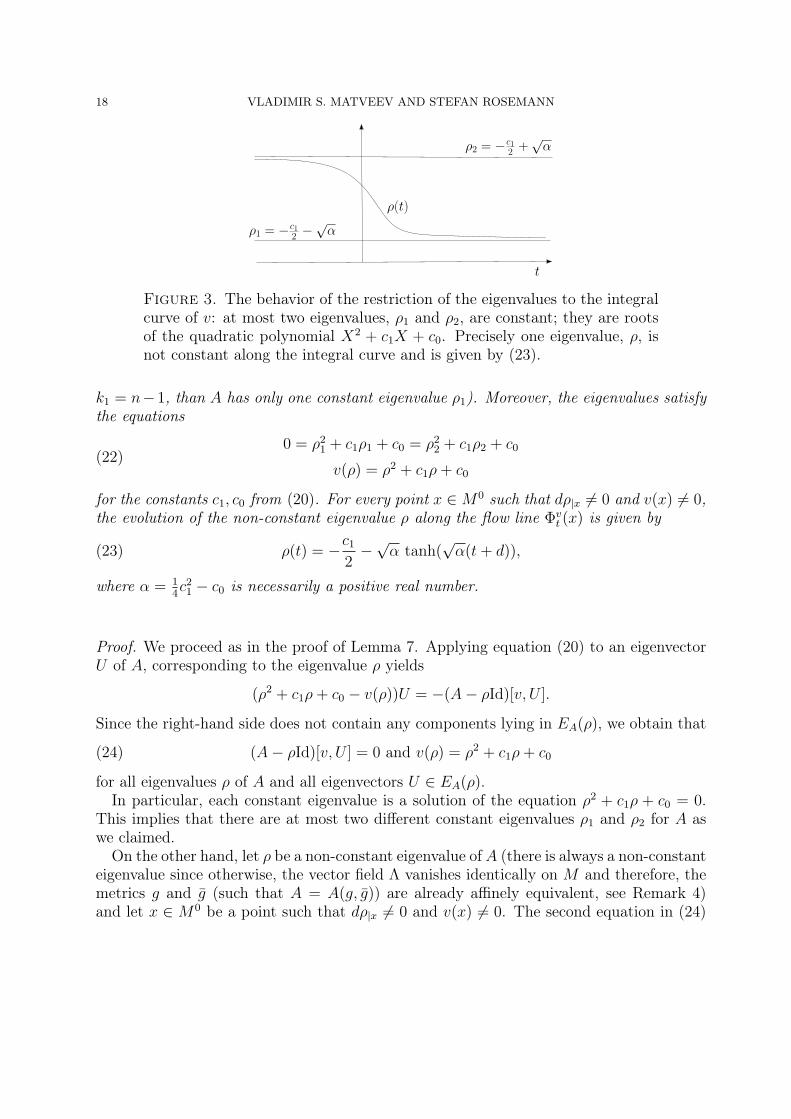
18 VLADIMIR S. MATVEEV AND STEFAN ROSEMANN
ρ(t)
ρ2 = −c12
+√
α
ρ1 = −c12−
√
α
t
Figure 3. The behavior of the restriction of the eigenvalues to the integralcurve of v: at most two eigenvalues, ρ1 and ρ2, are constant; they are rootsof the quadratic polynomial X2 + c1X + c0. Precisely one eigenvalue, ρ, isnot constant along the integral curve and is given by (23).
k1 = n−1, than A has only one constant eigenvalue ρ1). Moreover, the eigenvalues satisfythe equations
0 = ρ21 + c1ρ1 + c0 = ρ2
2 + c1ρ2 + c0
v(ρ) = ρ2 + c1ρ+ c0(22)
for the constants c1, c0 from (20). For every point x ∈M0 such that dρ|x 6= 0 and v(x) 6= 0,the evolution of the non-constant eigenvalue ρ along the flow line Φv
t (x) is given by
ρ(t) = −c12−√α tanh(
√α(t+ d)),(23)
where α = 14c21 − c0 is necessarily a positive real number.
Proof. We proceed as in the proof of Lemma 7. Applying equation (20) to an eigenvectorU of A, corresponding to the eigenvalue ρ yields
(ρ2 + c1ρ+ c0 − v(ρ))U = −(A− ρId)[v, U ].
Since the right-hand side does not contain any components lying in EA(ρ), we obtain that
(A− ρId)[v, U ] = 0 and v(ρ) = ρ2 + c1ρ+ c0(24)
for all eigenvalues ρ of A and all eigenvectors U ∈ EA(ρ).In particular, each constant eigenvalue is a solution of the equation ρ2 + c1ρ + c0 = 0.
This implies that there are at most two different constant eigenvalues ρ1 and ρ2 for A aswe claimed.
On the other hand, let ρ be a non-constant eigenvalue of A (there is always a non-constanteigenvalue since otherwise, the vector field Λ vanishes identically on M and therefore, themetrics g and g (such that A = A(g, g)) are already affinely equivalent, see Remark 4)and let x ∈ M0 be a point such that dρ|x 6= 0 and v(x) 6= 0. The second equation in (24)
PROOF OF THE YANO-OBATA CONJECTURE FOR h-PROJECTIVE TRANSFORMATIONS 19
shows that the restriction of ρ to the flow line Φvt (x) of v (i.e., ρ(t) := ρ(Φv
t (x)) satisfiesthe ordinary differential equation
ρ = ρ2 + c1ρ+ c0, where ρ stays for ddtρ.(25)
This ODE can be solved explicitly; the solution (depending on the parameters c1, c0) is
given by the following list. We put α =c214− c0.
• For α < 0, the non-constant solutions of equation (25) are of the form
−c12−
√−α tan(
√−α(−t+ d)).
• For α > 0, the non-constant solutions of equation (25) take the form
−c12−
√α tanh(
√α(t+ d)) or − c1
2−√α coth(
√α(t+ d)).
• For α = 0, the non-constant solutions of equation (25) are given by
−c12− 1
t+ d.
Since the degree of mobility is equal to 2, we can apply Lemma 6 to obtain that the flowΦv
t maps M0 onto M0. It follows that ρ(t) satisfies equation (25) for all t ∈ R. However,the only solution of (25) which does not reach infinity in finite time is
−c12−√α tanh(
√α(t+ d)),
where α =c214− c0 is necessarily a positive real number.
We obtain that the non-constant eigenvalues of A satisfy equation (23), in particular, theirimages contain the open interval (− c1
2−√
α,− c12+√α). Suppose that there are two different
non-constant eigenvalues ρ = − c12−√
α tanh(√α(t+d)) and ρ = − c1
2−√
α tanh(√α(t+ d))
of A. Then we can find points x0, x1, x2 ∈ M such that ρ(x0) < ρ(x1) < ρ(x2). Thiscontradicts the global ordering of the eigenvalues of A, see Theorem 3(1). It follows thatA has precisely one non-constant eigenvalue ρ. This eigenvalue restricted to flow lines ofv satisfies equation (23). By Corollary 2, the multiplicity of ρ is equal to two. We obtainthat there must be at least one constant eigenvalue of A. Finally, Lemma 8 is proven. �
Corollary 5. In the notation above, all eigenvalues ρ1, ρ, ρ2 are smooth functions on themanifold.
Proof. The eigenvalues ρ1, ρ2 are constant and are therefore smooth. The non-constanteigenvalue ρ is equal to 1
2traceA− k1ρ1 − (n− 1− k1)ρ2 and is therefore also smooth. �
Lemma 9. Let A have only one non-constant eigenvalue denoted by ρ. On Mdρ6=0 :={x ∈ M : dρ|x 6= 0}, the vector fields Λ and Λ are eigenvectors of A corresponding to theeigenvalue ρ, i.e., EA(ρ) = span{Λ, Λ}.Moreover, Mdρ6=0 is open and dense in M and Λ(ρ) 6= 0 on Mdρ6=0.
20 VLADIMIR S. MATVEEV AND STEFAN ROSEMANN
Remark 13. Note that the second part of the assertion above is still true even locally andeven if there are more than just one non-constant eigenvalue. The proof is based on thesame idea but is technically more complicated and will be published elsewhere.
Proof. First of all, since ρ is the only non-constant eigenvalue of A and ρ has multiplicityequal to 2 (see Corollary 2), we obtain Λ = 1
4grad traceA = 1
2grad ρ.
By Proposition 1, Λ is an eigenvector of A corresponding to the eigenvalue ρ. Since theeigenspaces of A are invariant with respect to the complex structure J , we immediatelyobtain EA(ρ) = span{Λ, Λ}. Moreover, since grad ρ is proportional to Λ, we have Λ(ρ) = 0and Λ(ρ) 6= 0 on Mdρ6=0.
Obviously, Mdρ6=0 is an open subset of M . As we explained above, dρ|x = 0, if and onlyif Λ(x) = Λ(x) = 0. Then, M \Mdρ6=0 coincides with the set of zeros of the non-trivialKilling vector field Λ. We obtain that Mdρ6=0 is dense in M . �
Let us now consider the critical points of the non-constant eigenvalue ρ:
Lemma 10. At every x such that dρ|x = 0, ρ takes its maximum or minimum values
ρ = − c12± √
α, where α =c214− c0 and c1, c0 are the constants from the equation (20).
Moreover, v 6= 0 on Mdρ6=0.
Proof. Since the subsets Mv 6=0 and Mdρ6=0 are both open and dense in M (see Corollary3 and Lemma 9), we obtain that M1 = Mv 6=0 ∩Mdρ6=0 is open and dense in M as well.Equation (23) shows that − c1
2−√
α < ρ(x) < − c12
+√α for all x ∈M1. Since M1 is dense,
we obtain
−c12−√α ≤ ρ(x) ≤ −c1
2+√α
for all x ∈ M . Now suppose that dρ|x = 0 for some x ∈ M . It follows from equation (22)that ρ(x) satisfies 0 = dρ|x(v) = ρ(x)2 + c1ρ(x) + c0, hence, ρ(x) is equal to the maximumor minimum value of ρ. Now suppose v(x) = 0. By (22), ρ takes its maximum or minimumvalue at x. It follows that dρ|x = 0. �
5.2. Metric components on integral manifolds of span{Λ, Λ}. By Lemma 8, A hasprecisely one non-constant eigenvalue ρ and at most two constant eigenvalues ρ1 and ρ2.The goal of this section is to calculate the components of the restriction of the metric g tothe integral manifolds of the eigenspace distribution EA(ρ) = span{Λ, Λ}. In order to doit, we split the tangent bundle on Mdρ6=0 into the direct product of two distributions:
D1 := span{Λ} and D2 := D⊥1 = span{Λ} ⊕ EA(ρ1) ⊕ EA(ρ2)
First let us show
Lemma 11. The distributions D1, D2 and EA(ρ) are integrable on Mdρ6=0. Moreover,integral manifolds of D1 and EA(ρ) are totally geodesic.
Proof. Since Λ is a gradient, the distributionD2 is integrable. On the other hand, Corollary4 immediately implies that EA(ρ) is integrable. The distribution D1 is one-dimensionaland is therefore integrable. In order to show that the integral manifolds of D1 and EA(ρ)
PROOF OF THE YANO-OBATA CONJECTURE FOR h-PROJECTIVE TRANSFORMATIONS 21
are totally geodesic, we consider the (quadratic in velocities) integrals I0, I1, I2 : TM → R
given by
I0(ζ) = g(Λ, ζ)2, I1(ζ) =(
dk1−1
dtk1−1Ft(ζ))
|t=ρ1 and I2(ζ) =(
dk2−1
dtk2−1Ft(ζ))
|t=ρ2 ,(26)
where 2k1, 2k2 are the multiplicities of the constant eigenvalues ρ1, ρ2 of A.If s : TM → R is a quadratic polynomial in the velocities, we define the nullity of s by
null s := {ζ ∈ TM : s(ζ) = 0}.In the orthonormal frame of eigenvectors of A from the proof of Theorem 3, the integralsFt are given by (10), and it is easy to see that
nullI1 = EA(ρ)⊕EA(ρ2), nullI2 = EA(ρ)⊕EA(ρ1) and nullI0 = span{Λ}⊕EA(ρ1)⊕EA(ρ2).
It follows that D1 = nullI0 ∩ nullI1 ∩ nullI2 and EA(ρ) = nullI1 ∩ nullI2. Since thefunctions are integrals, if γ(0) ∈ nullIi , then γ(t) ∈ nullIi for all t. Then, every geodesicγ such that γ(0) ∈ D1 (resp. EA(ρ)) remains tangent to D1 (resp. EA(ρ)). Thus, theintegral manifolds of D1 and EA(ρ) are totally geodesic. �
Let us introduce local coordinates x1, x2, ..., x2n in a neighborhood of a point of Mdρ6=0
such that (for all constants C1, ..., C2n) the equation x1 = C1 defines an integral manifoldof D2 and the system {xi = Ci}i=2,...,2n defines an integral manifold of D1. In thesecoordinates, the metric g has the block-diagonal form
g = g11dx1 ⊗ dx1 +
2n∑
i,j=2
gijdxi ⊗ dxj.
In what follows we call such coordinates adapted to the decomposition TM|Mdρ6=0= D1⊕D2.
Let us show that the h-projective vector field v splits into two independent componentswith respect to this decomposition:
Lemma 12. In the coordinates x1, x2, ..., x2n adapted to the decomposition TM|Mdρ6=0=
D1 ⊕D2, the h-projective vector field v is given by
(27) v = v1(x1)∂1︸ ︷︷ ︸
=:v1∈D1
+ v2(x2, ..., x2n)∂2 + ...+ v2n(x2, ..., x2n)∂2n︸ ︷︷ ︸
=:v2∈D2
Proof. Since Λ is an eigenvector of A corresponding to the non-constant eigenvalue ρ, thefirst equation in (24) implies that
[v, Λ] = f Λ + hΛ
for some functions f, h. If we apply dρ to both sides of the equation above, we obtainΛ(v(ρ)) = Λ(ρ2 + c1ρ + c0) = 0 on the left-hand side and hΛ(ρ) on the right-hand side.Since Λ(ρ) 6= 0 on Mdρ6=0, we necessarily have h = 0. By definition v is holomorphic andsince Λ = JΛ, we see that the equations
[v, Λ] = f Λ and [v,Λ] = fΛ(28)

22 VLADIMIR S. MATVEEV AND STEFAN ROSEMANN
are satisfied.For an eigenvector U of A, corresponding to some constant eigenvalue µ, the first equationin (24) shows that
[v, U ] ∈ EA(µ).(29)
For each index i ≥ 2, ∂i is contained in D2. On the other hand, ∂1 is always proportionalto Λ. We obtain
∂i ∼ Λ mod EA(ρ1) ⊕ EA(ρ2) and ∂1 ∼ Λ.
Using equation (28) and equation (29), we see that
[v, ∂i] ∈ D2 for all i ≥ 2 and [v, ∂1] ∈ D1.
This means that ∂iv1 = 0 and ∂1v
i = 0 for all i ≥ 2. Hence,
v = (v1(x1), v2(x2, ..., x2n), ..., v2n(x2, ..., x2n))
as we claimed. �
Let us write v = v1 + v2 with respect to the decomposition TM|Mdρ6=0= D1 ⊕D2 (as in
(27)). The vector fields v1 and v2 are well-defined and smooth on Mdρ6=0. By Lemma 12,we have [v1, v2] = 0.
Lemma 13. The non-constant eigenvalue ρ satisfies the equation v1(ρ) = ρ2 + c1ρ + c0and the evolution of ρ along the flow-lines of v1 is given by equation (23). Moreover, v1 isa non-vanishing complete vector field on Mdρ6=0.
Proof. Since by Proposition 1 and Lemma 9 we have dρ(V ) = 0 for all V ∈ D2, we havev2(ρ) = 0 and, hence, v1(ρ) = v(ρ) = ρ2 + c1ρ + c0. Using Lemma 12, we obtain that therestriction of ρ on the flow line Φv1
t (x) coincides with the restriction of ρ on Φvt (x) for all
x ∈ Mdρ6=0. Therefore the evolution of ρ along flow lines of v1 is again given by equation(23).Let us assume that v1(x) = 0 for some point x ∈ Mdρ6=0. We obtain that 0 = ρ(x)2 +c1ρ(x)+ c0, which implies that ρ(x) is a maximum or minimum value of ρ (see Lemma 10).It follows that dρ|x = 0, contracting our assumptions.Finally, let us show that v1 is complete. Take a maximal integral curve σ : (a, b) →Mdρ6=0
of v1 and assume b < ∞. Since M is closed, there exists a sequence {bn} ⊂ (a, b),converging to b such that limn → ∞σ(bn) = y for some y ∈ M . Then, y ∈ M \Mdρ6=0 sinceotherwise the maximal interval (a, b) of σ can be extended beyond b. Then, dρ|y = 0, andLemma 10 implies that ρ(y) is equal to the minimum value − c1
2− √
α. We obtain thatlimn → ∞ρ(σ(bn)) = − c1
2− √
α. On the other hand, formula (23) shows that this valuecannot be obtained in finite time b < ∞. This gives us a contradiction implying v1 is acomplete vector field on Mdρ6=0. �
Let us now calculate the restriction of the metric g to the integral manifolds of thedistribution EA(ρ) = span{v1, Λ}.
PROOF OF THE YANO-OBATA CONJECTURE FOR h-PROJECTIVE TRANSFORMATIONS 23
Lemma 14. In a neighborhood of each point of Mdρ6=0, it is possible to choose the coordi-nates t = x1, x2, ..., x2n adapted to the decomposition TM|Mdρ6=0
= D1 ⊕D2 in such a way,
that v1 = ∂1, Λ = ∂2 and
g =
h 0 0 . . . 00 g(Λ,Λ) ∗ . . . ∗0 ∗ ∗ . . . ∗...
......
...0 ∗ ∗ . . . ∗
.(30)
The functions h = g(v1, v1), g(Λ,Λ) and ρ depend on the first coordinate t only and aregiven explicitly by the formulas
h(t) = D e(C−c1)t
cosh2(√
α(t+d)),
g(Λ,Λ) = ρ2
4h(where ρ = dρ
dt) and
ρ(t) = − c12−√
α tanh(√α(t+ d)).
(31)
The constants α > 0 and C in equation (31) are defined as α =c214− c0 and C = −n−1
2c1 −
(2k1 + 1− n)√α+ (n+ 1)β, where D > 0, d, β, c1, c0 ∈ R and 2k1 is the multiplicity of the
constant eigenvalue ρ1. The constants c1, c0 are the same as in equation (20). Moreover,c1, c0 and β are global constants i.e., they are the same for each coordinate system of theabove type.
Proof. In a neighborhood of an arbitrary point ofMdρ6=0, let us introduce a chart x1, x2, ..., x2n,adapted to the decomposition TM|Mdρ6=0
= D1⊕D2. By Lemma 12 and Lemma 13, we canchoose these coordinates such that the flow line parameter t of v1 coincides with x1 (i.e.,such that the first component of v in the coordinate system equals ∂
∂x1 ). By (28), we have[v, Λ] ∈ D2. Moreover, [v2, Λ] ∈ D2 since D2 is integrable. It follows that [v1, Λ] ∈ D2.On the other hand, since v1 = fΛ for some function f and [Λ, Λ] = 0, we obtain that[v1, Λ] = −Λ(f)Λ ∈ D1, implying
[v1, Λ] = 0.
It follows, that we can choose the second coordinate x2 in such a way that Λ = ∂2.Next let us show that h = g11 depends on the first coordinate of the adapted chart only.For this, let I be an integral of second order for the geodesic flow of g such that I is block-diagonal with respect to the adapted coordinates t, x2, ..., x2n. For the moment we adoptthe convention that latin indices run from 2 to 2n such that I, considered as a polynomialon T ∗M , can be written as I = I11p2
1+I ijpipj. We calculate the poisson bracket 0 = {H, I}to obtain the equations
0 = I ik∂kg11 − gik∂kI
11 for all i = 2, ..., 2n.(32)
Inserting integrals I of special type, we can impose restrictions on the metric. Obviouslythe integrals I0, I1, I2 defined in equation (26) are block-diagonal. On the other hand, in
24 VLADIMIR S. MATVEEV AND STEFAN ROSEMANN
the proof of Lemma 11 it was shown that they satisfy nullI1 = EA(ρ) ⊕ EA(ρ2), nullI2 =EA(ρ) ⊕ EA(ρ1) and nullI0 = span{Λ} ⊕ EA(ρ1) ⊕ EA(ρ2). It follows that the integralF = I0+I1+I2 is block-diagonal and that its nullity is equal to D1. Then F can be writtenas F ijpipj and the matrix (F ij)i,j≥2 is invertible at each point where the coordinates aredefined. Replacing the integral I in equation (32) with F yields
∂ig11 = 0
for all 2 ≤ i ≤ 2n hence, the metric component g11 = (g11)−1 depends on t only.Now let us show the explicit dependence of the functions h, ρ and g(Λ,Λ) on the parametert. We already know that h = g11 and ρ depend on t only (for ρ this follows from Proposition1 and Lemma 9) and by Lemma 13, the dependence of ρ on the first coordinate t is givenby equation (23).Recall that λ = 1
4traceA = 1
2ρ+ const. It follows that dλ = 1
2ρ dt and hence, Λ = gradλ =
ρ
2h∂1. We obtain
g(Λ,Λ) =ρ2
4h.
What is left is to clarify the dependence of the function h on the parameter t. Note that inthe coordinates t, x2, ..., x2n, the h-projective vector field v is given by v = ∂1 + v2. Let usdenote by h and ρ the derivatives of h and ρ with respect to the coordinate t and denotethe restriction of g to the distribution D2 by g. Then we calculate
Lvg = Lv1g + Lv2g = h dt⊗ dt+ Lv1 g + Lv2 g,(33)
where we used that v2(h) = 0 and Lv2dt = 0 which follows from [v1, v2] = 0 and [v2, ∂i] ∈ D2
for all i ≥ 2. Note that Lv1 g and Lv2 g do not contain any expressions involving dt ⊗ dxi,dxi ⊗ dt or dt ⊗ dt. On the other hand, we already know that Av given in formula (6)satisfies equation (21). After multiplication with g from the left, (21) can be written as
Lvg −trace(g−1 ◦ Lvg)
2(n+ 1)g = a+ βg
for a = g ◦ A and some constant β. Calculating the trace on both sides yields
Lvg = a+ (β +1
2trace(A+ βId))g = a+ ((n+ 1)β + ρ+ k1ρ1 + k2ρ2)g.
Now we can insert equation (33) on the left-hand side to obtain
h dt⊗ dt+ Lv1 g + Lv2 g = a+ ((n+ 1)β + ρ+ k1ρ1 + k2ρ2)g.(34)
Since equation (34) is in block-diagonal form, it splits up into two separate equations. Thefirst equation which belongs to the matrix entry on the upper left reads
h = (2ρ+ C)h, where we defined C = k1ρ1 + k2ρ2 + (n+ 1)β.
Integration of this differential equation yields
h(t) = DeCt+2R
ρdt = De(C−c1)t−2 ln(cosh(√
α(t+d)))
PROOF OF THE YANO-OBATA CONJECTURE FOR h-PROJECTIVE TRANSFORMATIONS 25
for α =c214−c0 > 0 and some constants d andD > 0. If we insert the formulas ρ1 = − c1
2−√
αand ρ2 = − c1
2+
√α for the constant eigenvalues in the definition of the constant C, we
obtain
C = −n− 1
2c1 − (2k1 + 1 − n)
√α+ (n+ 1)β.
Finally, Lemma 14 is proven. �
The formulas (31) in Lemma 14 show that the restriction
g|EA(ρ) =
(h 00 g(Λ,Λ)
)
(35)
of the metric to the integral manifolds of the distribution EA(ρ) = span{v1, Λ} (the co-ordinates are as in Lemma 14 i.e., ∂1 = v1 and ∂2 = Λ) depends on the global constantsc1, c0, k1 and β. The constants D and d are not interesting; they can depend a priori onthe particular choice of the coordinate neighborhood. Note that c1 and c0 are subject tothe condition α = c21/4 − c0 > 0. Now our goal is to show that we can impose furtherconstraints on the constants such that the only metric which is left is the metric of positiveconstant holomorphic sectional curvature. So far, we did not really use that the manifoldis closed, indeed, most of the statements listed above still would be true if this conditionis omitted. However, as the next lemma shows, the condition that M is closed imposesstrong restrictions on the constants from Lemma 14:
Lemma 15. The constants from the formulas (31) of Lemma 14 satisfy C = c1. Inparticular, the function h = g(v1, v1) has the form
h(t) =D
cosh2(√α(t+ d))
.(36)
Proof. First we will show that certain integral curves of v1 always have finite length. Letxmax and xmin be points where ρ takes its maximum and minimum values respectively. Weconsider a geodesic γ : [0, 1] → M joining the points γ(0) = xmax and γ(1) = xmin. Weagain consider the integrals I0, I1, I2 : TM → R given by (26). Since the Killing vector fieldΛ vanishes at xmax, we obtain that 0 = I0(γ(0)) = I0(γ(t)) for all t ∈ [0, 1]. By Lemma 13,ρ(xmax) is equal to the constant eigenvalue ρ2 = − c1
2+
√α. It follows that I2(ζ) = 0 for
all ζ ∈ TxmaxM , in particular, I2(γ(0)) = 0. This implies that I2(γ(t)) = 0 for all t ∈ [0, 1].Similarly, considering the point xmin, we obtain I1(γ(t)) = 0 for all t ∈ [0, 1]. In the proofof Lemma 11, we already remarked that the distribution D1 is equal to the intersection ofthe nullities of I0, I1 and I2. It follows that γ(t) is contained in D1 for all 0 < t < 1. Thisimplies that γ|(0,1) is a reparametrized integral curve σ : R → M of the complete vectorfield v1. In particular, the length
lg(σ) =
∫ +∞
−∞
√
g(σ(t), σ(t))dt =
∫ +∞
−∞
√
g(v1, v1)(σ(t))dt =
∫ +∞
−∞
√
h(t)dt(37)
of the curve σ is equal to the length lg(γ|[0,1]) of the geodesic γ. We obtain that lg(σ) is
finite. By equation (37), a necessary condition for lg(σ) to be finite is that√
h(t) → 0
26 VLADIMIR S. MATVEEV AND STEFAN ROSEMANN
when t→ ∞. Note that h(t) is given by the first equation in (31) (for some constants D, dthat can depend on the particular integral curve σ). From formula (31), we obtain that√
h(t) for t→ ∞ is asymptotically equal to
√
h(t) ∼ e
�C−c12√
α−1
�t.
The finiteness of lg(σ) now implies the condition
−C − c12√α
+ 1 > 0(38)
on the global constants given in equation (31). Let us find further conditions on theconstants. Since M is assumed to be closed, the holomorphic sectional curvature
KEA(ρ) =g(v1, R(v1, Λ)Λ)
g(v1, v1)g(Λ,Λ)=
R1212
h g(Λ,Λ)
of EA(ρ) has to be bounded on M . Since the integral manifolds of EA(ρ) are totallygeodesic (by Lemma 11), the sectional curvature KEA(ρ) is equal to the curvature of thetwo dimensional metric (35). After a straight-forward calculation using the formulas (31)for h and g(Λ,Λ), we obtain
KEA(ρ)(t) =1
4D
[
(−4c0 − C2 + 2Cc1)︸ ︷︷ ︸
=:γ1
e−(C−c1)t −(C − c1)2
︸ ︷︷ ︸
=:γ2
cosh(2√α(t+ d))e−(C−c1)t
−2(C − c1)√α
︸ ︷︷ ︸
=:γ3
sinh(2√α(t+ d))e−(C−c1)t
]
(39)
=:1
4D(γ1f1(t) + γ2f2(t) + γ3f3(t)).
Similar to the first part of the proof, we can consider the asymptotic behavior t → ∞ ofthe functions f2(t), f3(t) appearing as coefficients of the constants γ2, γ3 in formula (39).We substitute s = 2
√α(t+ d) and obtain
f2(s) ∼ cosh(s)e−C−c1
2√
αs ∼
t≫0e
�−C−c1
2√
α+1
�t (38)−→
t→∞∞,
f3(s) ∼ sinh(s)e−C−c1
2√
αs ∼
t≫0e
�−C−c1
2√
α+1
�t (38)−→
t→∞∞.
As we already have mentioned, the sectional curvatures of a closed manifold are boundedand hence, KEA(ρ)(t) must be finite when t approaches the limit t → ∞. Using theformulas for the asymptotic behavior of f2(t) and f3(t) given above, this condition imposesthe restriction γ2 = −γ3 on the constants in equation (39). Similarly, considering theasymptotic behaviour for t → −∞, we obtain γ2 = γ3. Note that the dominating part insinh(2
√α(t+ d)) now comes with the minus sign. It follows that γ2 = γ3 = 0, hence,
C − c1 = 0(40)
PROOF OF THE YANO-OBATA CONJECTURE FOR h-PROJECTIVE TRANSFORMATIONS 27
as we claimed. Inserting equation (40) in the first formula of (31), the metric componentg11 = h takes the form (36). Lemma 15 is proven. �
Remark 14. If we insert γ2 = γ3 = 0 and C = c1 in the formula (39) for the sectionalcurvature of EA(ρ), we obtain that KEA(ρ) = α
Dis constant and positive as we claimed.
5.3. Proof of Theorem 4. Our goal is to prove Theorem 4: we need to show the localexistence of a function µ and a constant B such that the system (14) is satisfied.
Lemma 16. At every point x ∈ M , the tensor A and the covariant differential ∇Λ aresimultaneously diagonalizable in an orthogonal basis. More precisely, let U ∈ EA(ρ1) andW ∈ EA(ρ2) be eigenvectors of A corresponding to the constant eigenvalues. Then weobtain
∇ΛΛ = (φ+ φψ)Λ,
∇ΛΛ = (φ+ φψ)Λ,
∇UΛ = g(Λ,Λ)ρ−ρ1
U,
∇W Λ = g(Λ,Λ)ρ−ρ2
W.
(41)
The functions φ and ψ are given by the formulas
φ =1
2
ρ
hand ψ =
1
2
h
h.(42)
Proof. Since the distribution D1 has totally geodesic integral manifolds (see Lemma 11),∇v1v1 is proportional to v1. Let us define two functions φ and ψ by setting
Λ =: φv1 and ∇v1v1 =: ψv1.(43)
It follows immediately that g(Λ,Λ) = φ2h. On the other hand, h = 2g(∇v1v1, v1) = 2ψh.Using the equations (31) in Lemma 14, we obtain
φ =1
2
ρ
hand ψ =
1
2
h
h.(44)
Note that the function φ has to be negative since ρ decreases along the flow-lines of v1
while it increases along the flow-lines of Λ = 12grad ρ. By direct calculation, we obtain
∇ΛΛ = φ∇v1(φv1) = φφv1 + φ2∇v1v1 = (φφ+ φ2ψ)v1 = (φ+ φψ)Λ.
From the equation above, the relation Λ = JΛ and the fact that Λ is a holomorphic vectorfield, we immediately obtain
∇ΛΛ = J∇ΛΛ = (φ+ φψ)Λ
and hence, the first two equations in (41) are proven.Now let U ∈ EA(ρ1) be an eigenvector of A corresponding to the constant eigenvalue ρ1.Using Proposition 1, we obtain
∇U Λ = −g(Λ,Λ)
ρ1 − ρJU + f Λ + fΛ and ∇ΛU = 0 mod EA(ρ1)(45)
28 VLADIMIR S. MATVEEV AND STEFAN ROSEMANN
for some functions f and f . The lie bracket of U and Λ is given by
[U, Λ] = f Λ + fΛ mod EA(ρ1).
Applying dρ to both sides of the equation above yields fΛ(ρ) = 0. Since Λ(ρ) 6= 0 on
Mdρ6=0, it follows that f = 0. On the other hand, the first equation in (45) shows that
1
2U(g(Λ,Λ)) = g(∇U Λ, Λ) = fg(Λ,Λ).
Since dg(Λ,Λ) is zero when restricted to the distribution D2 (as can be seen by using thecoordinates given in Lemma 14), the left-hand side of the equation above vanishes and
hence, f = 0. Inserting f = f = 0 in the first equation of (45), we obtain the thirdequation in (41). If we replace ρ1 and U by ρ2 and W ∈ EA(ρ2), the same arguments canbe applied to obtain the last equation in (41). Lemma 16 is proven. �
Let (M, g, J) be a closed, connected Riemannian Kahler manifold of real dimension2n ≥ 4 and of degree of mobility D(g) = 2. Let v be an essential h-projective vector fieldand t0 a real number, such that g = (Φv
t0)∗g is not already affinely equivalent to g. Let us
denote by A = A(g, g) the corresponding solution of equation (3).We want to show that any point of Mdρ6=0 has a small neighborhood such that in thisneighborhood there exist a function µ and a constant B < 0 such that the covariantdifferential ∇Λ satisfies the second equation
∇Λ = µId +BA(46)
in (14). By Lemma 16, at every point of Mdρ6=0, each eigenvector of A is an eigenvectorof ∇Λ. Since A has (at most) three different eigenvalues, equation (46) is equivalent toan inhomogeneous linear system of three equations on the two unknown real numbers µand B. Using formulas (41) from Lemma 16, we see that for x ∈ Mdρ6=0, ∇Λ satisfiesequation (46) for some numbers µ and B, if and only if the inhomogeneous linear systemof equations
µ+ ρB = φ+ φψ,
µ+ ρ1B = g(Λ,Λ)ρ−ρ1
,
µ+ ρ2B = g(Λ,Λ)ρ−ρ2
.
(47)
is satisfied. Now, according to Lemma 14 and Lemma 15, in a neighborhood of a point ofMdρ6=0, the functions ρ, g(Λ,Λ), h, φ and ψ are given explicitly by (31), (36) and (42). Letus insert these functions and the formulas − c1
2±√
α for the constant eigenvalues ρ1 < ρ2
(see Lemma 8) in (47). After a straight-forward calculation, we obtain that (47) is satisfiedfor
µ = −α( c12−√
α tanh(√α(t+ d)))
4D= B(c1 + ρ) and B = − α
4D.(48)
We see also that the constant B is negative (as we claimed in Section 2.2).
PROOF OF THE YANO-OBATA CONJECTURE FOR h-PROJECTIVE TRANSFORMATIONS 29
Using the equation λ = 14traceA = 1
2ρ + const, we obtain that µ given by (48) satisfies
dµ = Bdρ = 2Bdλ. Since Λ is the gradient of λ, this is easily seen to be equivalent to thethird equation in the system (14).
We have shown that in a neighborhood of almost every point of M , there exists asmooth function µ and a constant B < 0, such that the system (14) is satisfied for thetriple (A,Λ, µ).
If A is another element in Sol(g) with the corresponding vector field Λ, then A = aA+bIdfor some a, b ∈ R implying Λ = aΛ. By direct calculations we see that for an appropriatelocal function µ the triple (A, Λ, µ) satisfies the system (14) for the same constant B = B.Finally, Theorem 4 is proven.
6. Final step in the proof of Theorem 1
As we explained in Section 2.2, it is sufficient to prove Theorem 1 under the additionalassumption that the degree of mobility is equal to two. By Theorem 4, for every A ∈ Sol(g)with corresponding vector field Λ = 1
4grad traceA, in a neighborhood U(x) of almost every
point x ∈ M , there exists a local function µ : U(x) → R and a negative constant B suchthat the triple (A,Λ, µ) satisfies the system (14).
Now, in [7, §2.5] it was shown that under these assumptions the constant B is the samefor all such neighborhoods, implying that the system (14) is satisfied on the whole M (fora certain smooth function µ : M → R). Note that in view of the third equation of (14), µis not a constant (if A is chosen to be non-proportional to the identity on TM).
By direct calculation (differentiating µ and replacing the derivatives using the system(14)), we obtain
(∇∇µ)(Y, Z) = ∇Y (∇Zµ) −∇∇Y Zµeq. 3 of (14)
= 2Bg(Z,∇Y Λ)
eq. 2 of (14)= 2B(µg(Y, Z) +Bg(AY,Z)).
Then,
(∇∇∇µ)(X,Y, Z) = 2B((∇Xµ)g(Y, Z) +Bg((∇XA)Y, Z))
eq. 1 of (14)= B(2(∇Xµ)g(Y, Z) + 2Bg(Z,Λ)g(X,Y ) + 2Bg(Y,Λ)g(X,Z)
+2Bg(Z, Λ)g(JX, Y ) + 2Bg(Y, Λ)g(JX,Z)).
Inserting the third equation of (14), we obtain that µ satisfies the equation
(∇∇∇µ)(X,Y, Z) = B[2(∇Xµ)g(Y, Z) + (∇Zµ)g(X,Y ) + (∇Y µ)g(X,Z)
−(∇JZµ)g(JX, Y ) − (∇JY µ)g(JX,Z)](49)
for all X,Y, Z ∈ TM .Now by [48, Theorem 10.1], the existence of a non-constant solution of equation (49) withB < 0 on a closed, connected Riemannian Kahler manifold implies that the manifold haspositive constant holomorphic sectional curvature equal to −4B. Then, (M,−4Bg, J) canbe covered by (CP (n), gFS, J). Theorem 1 is proven.
30 VLADIMIR S. MATVEEV AND STEFAN ROSEMANN
References
[1] H. Akbar-Zadeh, Transformations holomorphiquement projectives des varietes hermitiennes et
kahleriennes, J. Math. Pures Appl. (9) 67, no. 3, 237–261, 1988[2] D. V. Alekseevsky, Groups of conformal transformations of Riemannian spaces, Math. USSR Sbornik,
18, 285–301, 1972[3] E. Beltrami, Risoluzione del problema: riportare i punti di una superficie sopra un piano in modo che
le linee geodetische vengano rappresentante da linee rette, Ann. di Mat., 1, no. 7, 185–204, 1865[4] A. V. Bolsinov, V. S. Matveev, Geometrical interpretation of Benenti’s systems, J. of Geometry and
Physics 44, no. 4, 489–506, 2003[5] A. V. Bolsinov, V. S. Matveev, Splitting and gluing lemmas for geodesically equivalent
pseudo-Riemannian metrics, accepted to Transactions of the American Mathematical Society,arXiv:math.DG/0904.0535.
[6] U. Dini, Sopra un problema che si presenta nella teoria generale delle rappresentazioni geografiche di
una superficie su un’altra, Ann. Mat., ser.2, 3(1869), 269–293.[7] A. Fedorova, V. Kiosak, V. Matveev, S. Rosemann, Every closed Kahler manifold with degree of
mobility ≥ 3 is (CP (n), gFubini−Study), arXiv:1009.5530v1 [math.DG], 2010[8] J. Ferrand, Action du groupe conforme sur une variete riemannienne., C. R. Acad. Sci. Paris Ser. I
Math. 318, no. 4, 347-350, 1994[9] G. Fubini, Sui gruppi trasformazioni geodetiche, Mem. Acc. Torino (29 53(1903), 261–313.
[10] S. Fujimura, Indefinite Kahler metrics of constant holomorphic sectional curvature, J. Math. KyotoUniv. 30, no. 3, 493–516, 1990
[11] I. Hasegawa, H-projective-recurrent Kahlerian manifolds and Bochner-recurrent Kahlerian manifolds,
Hokkaido Math. J. 3, 271–278, 1974[12] I. Hasegawa, S. Fujimura, On holomorphically projective transformations of Kaehlerian manifolds.
Math. Japon. 42, no. 1, 99–104, 1995[13] I. Hasegawa, K. Yamauchi, Infinitesimal projective transformations on tangent bundles with lift con-
nections, Sci. Math. Jpn. 57(2003), no. 3, 469–483.[14] H. Hiramatu, Riemannian manifolds admitting a projective vector field, Kodai Math. J. 3, no. 3,
397–406, 1980[15] H. Hiramatu, Integral inequalities in Kahlerian manifolds and their applications, Period. Math. Hun-
gar. 12, no. 1, 37–47, 1981[16] S. Ishihara, Holomorphically projective changes and their groups in an almost complex manifold,
Tohoku Math. J. (2) 9, 273–297, 1957[17] S. Ishihara, S. Tachibana, On infinitesimal holomorphically projective transformations in Kahlerian
manifolds, Tohoku Math. J. (2) 12, 77–101, 1960[18] S. Ishihara, S. Tachibana, A note on holomorphic projective transformations of a Kaehlerian space
with parallel Ricci tensor, Tohoku Math. J. (2) 13, 193–200, 1961[19] K. Kiyohara, Two classes of Riemannian manifolds whose geodesic flows are integrable, Mem. Amer.
Math. Soc. 130, no. 619, viii+143 pp., 1997[20] K. Kiyohara, P. J. Topalov, On Liouville integrability of h-projectively equivalent Kahler metrics,
Proc. Amer. Math. Soc. 139(2011), 231–242.[21] T. Levi-Civita, Sulle trasformazioni delle equazioni dinamiche, Ann. di math. 24, 255–300, 1896[22] A. Lichnerowicz, Geometry of groups of transformations. Translated from the French and edited by
Michael Cole, Noordhoff International Publishing, Leyden, 1977.[23] V. S. Matveev, P. J. Topalov, Trajectory equivalence and corresponding integrals, Regular and Chaotic
Dynamics 3, no. 2, 30–45, 1998[24] V. S. Matveev, Low-dimensional manifolds admitting metrics with the same geodesics, Contemporary
Mathematics 308, 229–243, 2002
PROOF OF THE YANO-OBATA CONJECTURE FOR h-PROJECTIVE TRANSFORMATIONS 31
[25] V. S. Matveev, Three-dimensional manifolds having metrics with the same geodesics, Topology 42,no. 6, 1371–1395, 2003
[26] V. S. Matveev, Hyperbolic manifolds are geodesically rigid, Invent. math. 151, no. 3, 579–609, 2003[27] V. S. Matveev, Die Vermutung von Obata fur Dimension 2, Arch. Math. 82, no. 4, 273–281, 2004[28] V. S. Matveev, Solodovnikov’s theorem in dimension two, Dokl. Akad. Nauk 396, no. 1, 25–27, 2004[29] V. S. Matveev, Closed manifolds admitting metrics with the same geodesics, Proceedings of SPT2004
(Cala Gonone). World Scientific, 198–208, 2005[30] V. S. Matveev, Lichnerowicz-Obata conjecture in dimension two, Comm. Math. Helv. 80, no. 3, 541–
570, 2005[31] V. S. Matveev, The eigenvalues of Sinjukov’s operator are globally ordered, Mathematical Notes,
77(2005) no. 3-4, 380-390.[32] V. S. Matveev, On degree of mobility for complete metrics, Adv. Stud. Pure Math. 43, 221–250, 2006[33] V. S. Matveev, Geometric explanation of the Beltrami theorem, Int. J. Geom. Methods Mod. Phys.
3, no. 3, 623–629, 2006[34] V. S. Matveev, Proof of the projective Lichnerowicz-Obata conjecture, J. Diff. Geom. 75, no. 3, 459–
502, 2007[35] J. Mikes, V. V. Domashev, On The Theory Of Holomorphically Projective Mappings Of Kaehlerian
Spaces, Math. Zametki 23, no. 2, 297–303, 1978[36] J. Mikes, Geodesic Mappings Of Affine-Connected And Riemannian Spaces, Journal of Math. Sciences
78, no. 3, 311–333, 1996[37] J. Mikes, Holomorphically projective mappings and their generalizations., J. Math. Sci. (New York)
89, no. 3, 1334–1353, 1998[38] T. Nagano, T. Ochiai, On compact Riemannian manifolds admitting essential projective transforma-
tions, J. Fac. Sci. Univ. Tokyo Sect. IA, Math. 33(1986) 233–246.[39] M. Obata, Riemannian manifolds admitting a solution of a certain system of differential equations,
Proc. U.S.-Japan Seminar in Differential Geometry (Kyoto, 1965) pp. 101–114.[40] M. Obata, The conjectures about conformal transformations, J. Diff. Geometry 6, 247–258, 1971[41] T. Otsuki, Y. Tashiro, On curves in Kaehlerian spaces, Math. Journal of Okayama University 4,
57–78, 1954[42] T. Sakaguchi, On the holomorphically projective correspondence between Kahlerian spaces preserving
complex structure , Hokkaido Mathematical Journal 33, no. 2, 203–212, 1974[43] R. Schoen, On the conformal and CR automorphism groups, Geom. Funct. Anal. 5, no. 2, 464–481,
1995[44] N. S. Sinjukov, Geodesic mappings of Riemannian spaces. (in Russian) “Nauka”, Moscow, 1979,
MR0552022, Zbl 0637.53020.[45] N. S. Sinyukov, Holomorphically projective mappings of special Kahlerian spaces, Mat. Zametki, 36,
no. 3, 417–423, 1984[46] H. Takeda, Hidehiro, Y. Watanabe, On Riemannian spaces with parallel Weyl’s projective curvature
tensor, Kyungpook Math. J. 12, 37–41, 1972[47] N. Tanaka, Projective connections and projective transformations, Nagoya Math. J. 12, 1–24, 1957[48] S. Tanno, Some Differential Equations On Riemannian Manifolds, J. Math. Soc. Japan 30, no. 3,
509–531, 1978[49] Y. Tashiro, On A Holomorphically Projective Correspondence In An Almost Complex Space, Math.
Journal of Okayama University 6, 147–152, 1956[50] P. J. Topalov and V. S. Matveev, Geodesic equivalence via integrability, Geometriae Dedicata 96,
91–115, 2003[51] P. J. Topalov, Geodesic Compatibility And Integrability Of Geodesic Flows, Journal of Mathematical
Physics 44, no. 2, 913–929, 2003[52] K. Yamauchi, On infinitesimal projective transformations, Hokkaido Math. J. 3(1974), 262–270.[53] K. Yano, On harmonic and Killing vector fields, Ann. of Math. (2) 55, 38–45, 1952
32 VLADIMIR S. MATVEEV AND STEFAN ROSEMANN
[54] K. Yano, Differential geometry on complex and almost complex spaces. International Series of Mono-graphs in Pure and Applied Mathematics, 49 A Pergamon Press Book. The Macmillan Co., New York1965 xii+326 pp.
[55] K. Yano, H. Hiramatu, Isometry Of Kaehlerian Manifolds To Complex Projective Spaces, J. Math.Soc. Japan 33, no. 1, 67–78, 1981
[56] Y. Yoshimatsu, H-projective connections and H-projective transformations, Osaka J. Math. 15, no.2, 435–459, 1978
![Isometries inspaces ofK¨ahler potentials - arXivarXiv:1702.05937v2 [math.CV] 13 Oct 2017 Isometries inspaces ofK¨ahler potentials∗ L´aszlo Lempert Department of Mathematics Purdue](https://img.pdfslide.us/doc/110x75/5f564da9946b2e2c712e0cf8/isometries-inspaces-ofkahler-potentials-arxiv-arxiv170205937v2-mathcv-13.jpg)