Introduction Transfer Function References

IntroductionFirst-order linear systems

Second-order linear systemsTransfer Function

Applications, conclusion and future workReferences

Second order systems

Filippo Sanfilippo

1

1Department of Engineering Cybernetics, Norwegian University of Science and Technology, 7491 Trondheim, Norway,[email protected]

Trial lecture at the Department of Electrical Engineering and Computer Science,University of Stavanger, Norway, 2017

Filippo Sanfilippo Second order systems




Introduction

About Me

Education:

PhD in Engineering Cybernetics,Norwegian University of Science andTechnology (NTNU), Norway

MSc in Computer Science Engineering,University of Siena, Italy

BSc degree in Computer ScienceEngineering, University of Catania, Italy

Mobility:

Visiting Fellow, Technical Aspects ofMultimodal Systems (TAMS),Department of Mathematics,Informatics and Natural Sciences,University of Hamburg, Hamburg,Germany

Visiting Student, School of Computingand Intelligent Systems, University ofUlster, Londonderry, United Kingdom

Granted with an Erasmus+ Sta↵Mobility for Teaching and Trainingproject

Activities:

Membership Development O�cer for the IEEENorway Section





Introduction

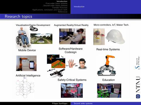
Research topics

Visualisation/Game Development Micro-controllers, IoT, Maker Tech.

Education

Augmented Reality/Virtual Reality

Mobile Device Software/Hardware Codesign

Real-time Systems

Artificial IntelligenceSafety-Critical Systems





Introduction

About Me

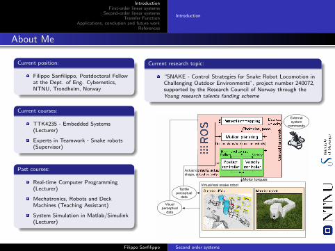
Current position:

Filippo Sanfilippo, Postdoctoral Fellowat the Dept. of Eng. Cybernetics,NTNU, Trondheim, Norway

Current courses:

TTK4235 - Embedded Systems(Lecturer)

Experts in Teamwork - Snake robots(Supervisor)

Past courses:

Real-time Computer Programming(Lecturer)

Mechatronics, Robots and DeckMachines (Teaching Assistant)

System Simulation in Matlab/Simulink(Lecturer)

Current research topic:

“SNAKE - Control Strategies for Snake Robot Locomotion inChallenging Outdoor Environments”, project number 240072,supported by the Research Council of Norway through theYoung research talents funding scheme

Virtual/real snake robotMamba robot

High-level control

Gazebo+RViz

External system

commandsPerception/mapping

Motion planning

Position controller

Obstacles, pose

Motor torques

Actual contacts, actual shape, actual velocity

Desired velocity

Desired shape/path (position, velocity)

Visual perceptual

data

Tactile perceptual

data

Cont

rol f

ram

ewor

k

Velocity controller

Position Velocity





First-order linear systems


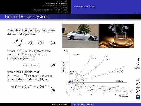
Canonical homogeneous first-orderdi↵erential equation:

⌧dy(t)

dt+ y(t) = f (t), (1)

where ⌧ 6= 0 is the system timeconstant. The characteristicequation is given by:

⌧�+ 1 = 0, (2)

which has a single root,� = �1/⌧ . The system responseto an initial condition y(0) is:

yh(t) = y(0)e�t = y(0)e�t/⌧ ,(3)






First-order linear systems: s-plane












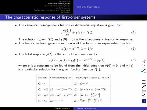
The characteristic response of first-order systems

The canonical homogeneous first-order di↵erential equation is given by:

⌧dy(t)

dt+ y(t) = f (t). (4)

The solution (given f (t) and y(0) = 0) is the characteristic first-order response.The first-order homogeneous solution is of the form of an exponential function:

yh(t) = e��t ,� = 1/⌧. (5)

The total response y(t) is the sum of two components:

y(t) = yh(t) + yp(t) = ce�t/⌧ + yp(t), (6)

where c is a constant to be found from the initial condition y(0) = 0, and yp(t)is a particular solution for the given forcing function f (t).





Second-order linear systemsStandard terms and pole locationsSignificant cases

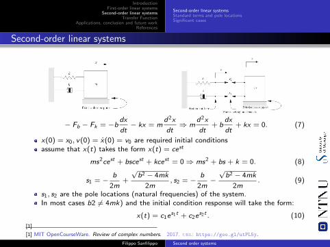
Second-order linear systems

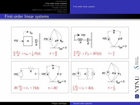
� Fb � Fk = �bdx

dt� kx = m

d2x

dt) m

d2x

dt+ b

dx

dt+ kx = 0. (7)

x(0) = x0, v(0) = x(0) = v0 are required initial conditionsassume that x(t) takes the form x(t) = cest

ms2cest + bscest + kcest = 0 ) ms2 + bs + k = 0. (8)

s1 = �b

2m+

pb2 � 4mk

2m, s2 = �

b

2m�

pb2 � 4mk

2m. (9)

s1, s2 are the pole locations (natural frequencies) of the system.In most cases b2 6= 4mk) and the initial condition response will take the form:

x(t) = c1es1t + c2e

s2t . (10)

[1]

[1] MIT OpenCourseWare. Review of complex numbers. 2017. url: https://goo.gl/utPL5y.


https://goo.gl/utPL5y





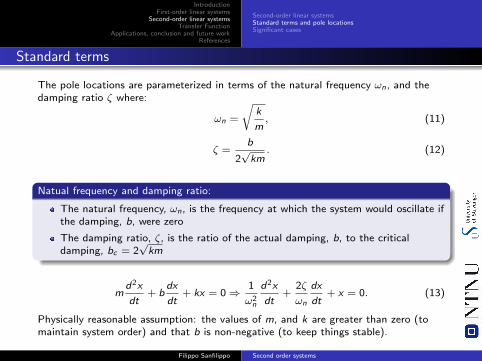
Standard terms

The pole locations are parameterized in terms of the natural frequency !n, and thedamping ratio ⇣ where:

!n =

rk

m, (11)

⇣ =b

2pkm

. (12)

Natual frequency and damping ratio:

The natural frequency, !n, is the frequency at which the system would oscillate ifthe damping, b, were zero

The damping ratio, ⇣, is the ratio of the actual damping, b, to the criticaldamping, bc = 2

pkm

md2x

dt+ b

dx

dt+ kx = 0 )

1

!2n

d2x

dt+

2⇣

!n

dx

dt+ x = 0. (13)

Physically reasonable assumption: the values of m, and k are greater than zero (tomaintain system order) and that b is non-negative (to keep things stable).






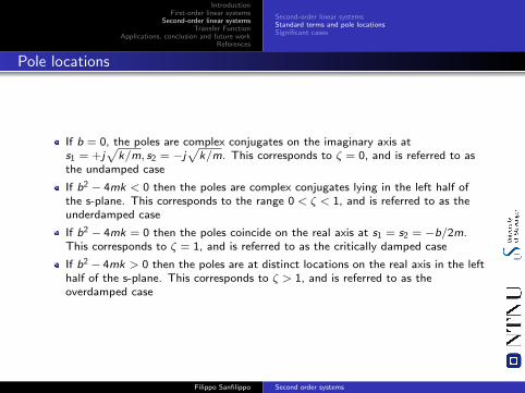
Pole locations

If b = 0, the poles are complex conjugates on the imaginary axis ats1 = +j

pk/m, s2 = �j

pk/m. This corresponds to ⇣ = 0, and is referred to as

the undamped case

If b2 � 4mk < 0 then the poles are complex conjugates lying in the left half ofthe s-plane. This corresponds to the range 0 < ⇣ < 1, and is referred to as theunderdamped case

If b2 � 4mk = 0 then the poles coincide on the real axis at s1 = s2 = �b/2m.This corresponds to ⇣ = 1, and is referred to as the critically damped case

If b2 � 4mk > 0 then the poles are at distinct locations on the real axis in the lefthalf of the s-plane. This corresponds to ⇣ > 1, and is referred to as theoverdamped case






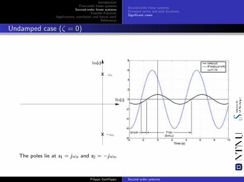
Undamped case (⇣ = 0)

The poles lie at s1 = j!n and s2 = �j!n.






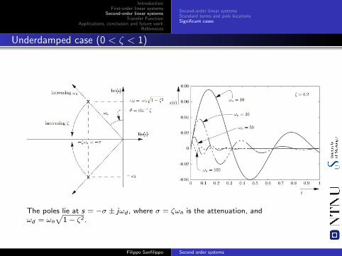
Underdamped case (0 < ⇣ < 1)

The poles lie at s = �� ± j!d , where � = ⇣!n is the attenuation, and!d = !n

p1� ⇣2.






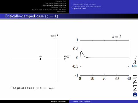
Critically-damped case (⇣ = 1)

The poles lie at s1 = s2 = �!n.






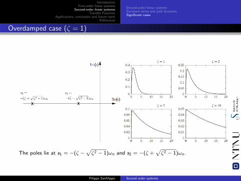
Overdamped case (⇣ = 1)

The poles lie at s1 = �(⇣ �p

⇣2 � 1)!n and s2 = �(⇣ +p

⇣2 � 1)!n.





Transfer FunctionMass-spring-damper systemMass-Spring-Damper in Simulink

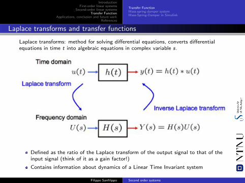
Laplace transforms and transfer functions

Laplace transforms: method for solving di↵erential equations, converts di↵erentialequations in time t into algebraic equations in complex variable s.

Defined as the ratio of the Laplace transform of the output signal to that of theinput signal (think of it as a gain factor!)

Contains information about dynamics of a Linear Time Invariant system






Mass-spring-damper system






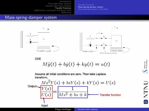
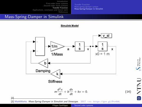
Mass-Spring-Damper in Simulink

md2x

dt+ b

dx

dt+ kx = 0. (14)

[2]

[2] MathWorks. Mass-Spring-Damper in Simulink and Simscape. 2017. url: https://goo.gl/Ftr6hK.


https://goo.gl/Ftr6hK




ApplicationsConclusion and future work

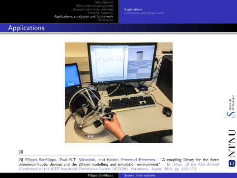
Applications

[3]

[3] Filippo Sanfilippo, Paul B.T. Weustink, and Kristin Ytterstad Pettersen. “A coupling library for the forcedimension haptic devices and the 20-sim modelling and simulation environment”. In: Proc. of the 41st AnnualConference of the IEEE Industrial Electronics Society (IECON), Yokohama, Japan. 2015, pp. 168–173.






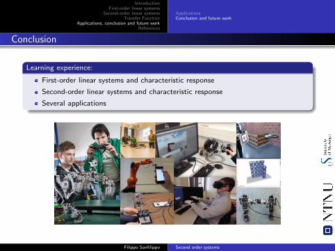
Conclusion

Learning experience:

First-order linear systems and characteristic response

Second-order linear systems and characteristic response

Several applications






Thank you for your attention

Contact:

F. Sanfilippo, Department of Engineering Cybernetics, Norwegian University ofScience and Technology, 7491 Trondheim, Norway, [email protected]

[4–6]

[4] Filippo Sanfilippo et al. “Virtual functional segmentation of snake robots for perception-driven obstacle-aidedlocomotion”. In: Proc. of the IEEE Conference on Robotics and Biomimetics (ROBIO), Qingdao, China. 2016,pp. 1845–1851.

[5] Filippo Sanfilippo et al. “A review on perception-driven obstacle-aided locomotion for snake robots”. In: Proc.of the 14th International Conference on Control, Automation, Robotics and Vision (ICARCV), Phuket, Thailand.2016, pp. 1–7.

[6] Filippo Sanfilippo et al. “Perception-driven obstacle-aided locomotion for snake robots: the state of the art,challenges and possibilities”. In: Applied Sciences 7.4 (2017), p. 336.





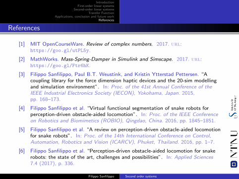
References

[1] MIT OpenCourseWare. Review of complex numbers. 2017. url:https://goo.gl/utPL5y.

[2] MathWorks. Mass-Spring-Damper in Simulink and Simscape. 2017. url:https://goo.gl/Ftr6hK.

[3] Filippo Sanfilippo, Paul B.T. Weustink, and Kristin Ytterstad Pettersen. “Acoupling library for the force dimension haptic devices and the 20-sim modellingand simulation environment”. In: Proc. of the 41st Annual Conference of theIEEE Industrial Electronics Society (IECON), Yokohama, Japan. 2015,pp. 168–173.

[4] Filippo Sanfilippo et al. “Virtual functional segmentation of snake robots forperception-driven obstacle-aided locomotion”. In: Proc. of the IEEE Conferenceon Robotics and Biomimetics (ROBIO), Qingdao, China. 2016, pp. 1845–1851.

[5] Filippo Sanfilippo et al. “A review on perception-driven obstacle-aided locomotionfor snake robots”. In: Proc. of the 14th International Conference on Control,Automation, Robotics and Vision (ICARCV), Phuket, Thailand. 2016, pp. 1–7.

[6] Filippo Sanfilippo et al. “Perception-driven obstacle-aided locomotion for snakerobots: the state of the art, challenges and possibilities”. In: Applied Sciences7.4 (2017), p. 336.


https://goo.gl/utPL5y

https://goo.gl/Ftr6hK

Documents

Introduction Transfer Function References