Embed Size (px)
Citation preview
8/14/2019 Introduction to Timefrequencyanalysis Ssp&Mm 2013-14
http://slidepdf.com/reader/full/introduction-to-timefrequencyanalysis-sspmm-2013-14 1/61
Introduction to
Time-Frequency Analysis
Lorenzo Galleani
Department of Electronics and Telecommunications, Politecnico di Torino
Statistical Signal Processing and Multimedia
8/14/2019 Introduction to Timefrequencyanalysis Ssp&Mm 2013-14
http://slidepdf.com/reader/full/introduction-to-timefrequencyanalysis-sspmm-2013-14 2/61
2
Time-Frequency Analysis (TFA)
• Born around the middle of 1900• “Boom” around 1980
• Extension of classical frequency analysis
8/14/2019 Introduction to Timefrequencyanalysis Ssp&Mm 2013-14
http://slidepdf.com/reader/full/introduction-to-timefrequencyanalysis-sspmm-2013-14 3/61
3
Classical Frequency Analysis 1/2
• Fourier: Engineer • 1700-1800
• Decomposition of a signal in a sum ofsinusoids
• Heat transfer
8/14/2019 Introduction to Timefrequencyanalysis Ssp&Mm 2013-14
http://slidepdf.com/reader/full/introduction-to-timefrequencyanalysis-sspmm-2013-14 4/61
4
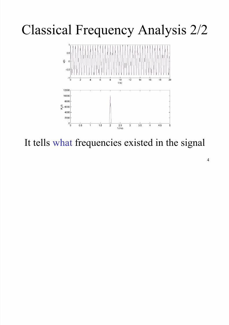
Classical Frequency Analysis 2/2
It tells what frequencies existed in the signal
8/14/2019 Introduction to Timefrequencyanalysis Ssp&Mm 2013-14
http://slidepdf.com/reader/full/introduction-to-timefrequencyanalysis-sspmm-2013-14 5/61
5
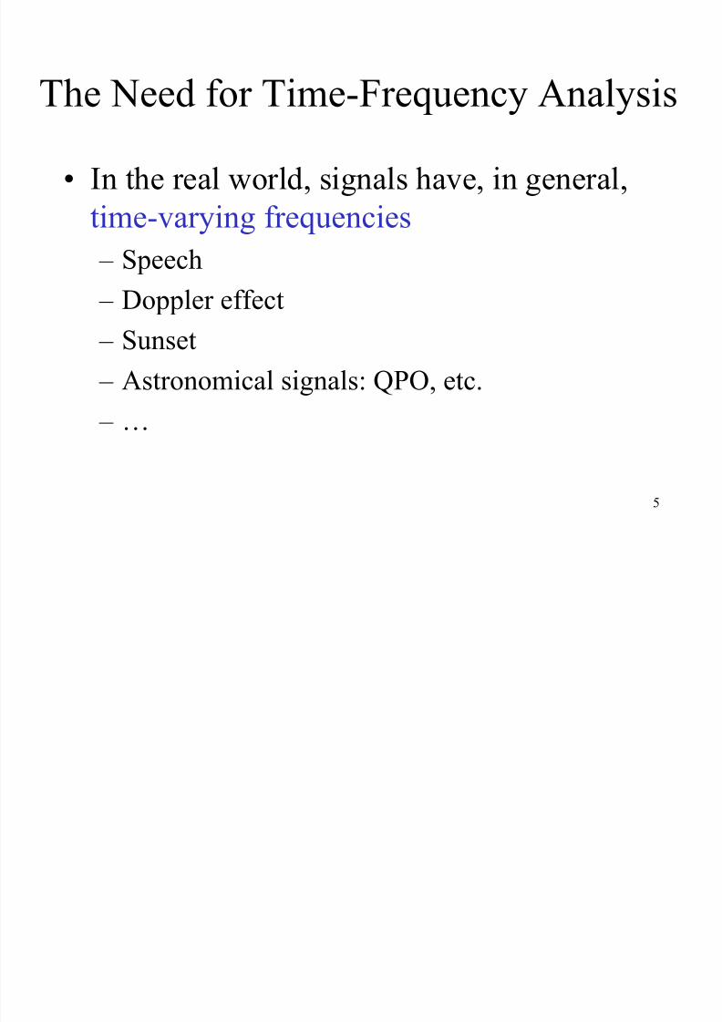
The Need for Time-Frequency Analysis
• In the real world, signals have, in general,time-varying frequencies
– Speech
– Doppler effect
– Sunset
– Astronomical signals: QPO, etc.
– …

8/14/2019 Introduction to Timefrequencyanalysis Ssp&Mm 2013-14
http://slidepdf.com/reader/full/introduction-to-timefrequencyanalysis-sspmm-2013-14 6/61
6
We want more
We want to know
what frequencies existed in the signal
and
when they existed
8/14/2019 Introduction to Timefrequencyanalysis Ssp&Mm 2013-14
http://slidepdf.com/reader/full/introduction-to-timefrequencyanalysis-sspmm-2013-14 7/61
7
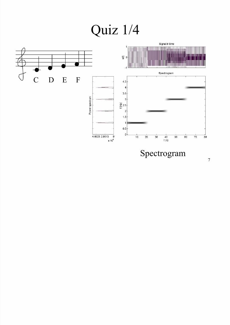
Quiz 1/4
C D E F
Spectrogram
8/14/2019 Introduction to Timefrequencyanalysis Ssp&Mm 2013-14
http://slidepdf.com/reader/full/introduction-to-timefrequencyanalysis-sspmm-2013-14 8/61
8
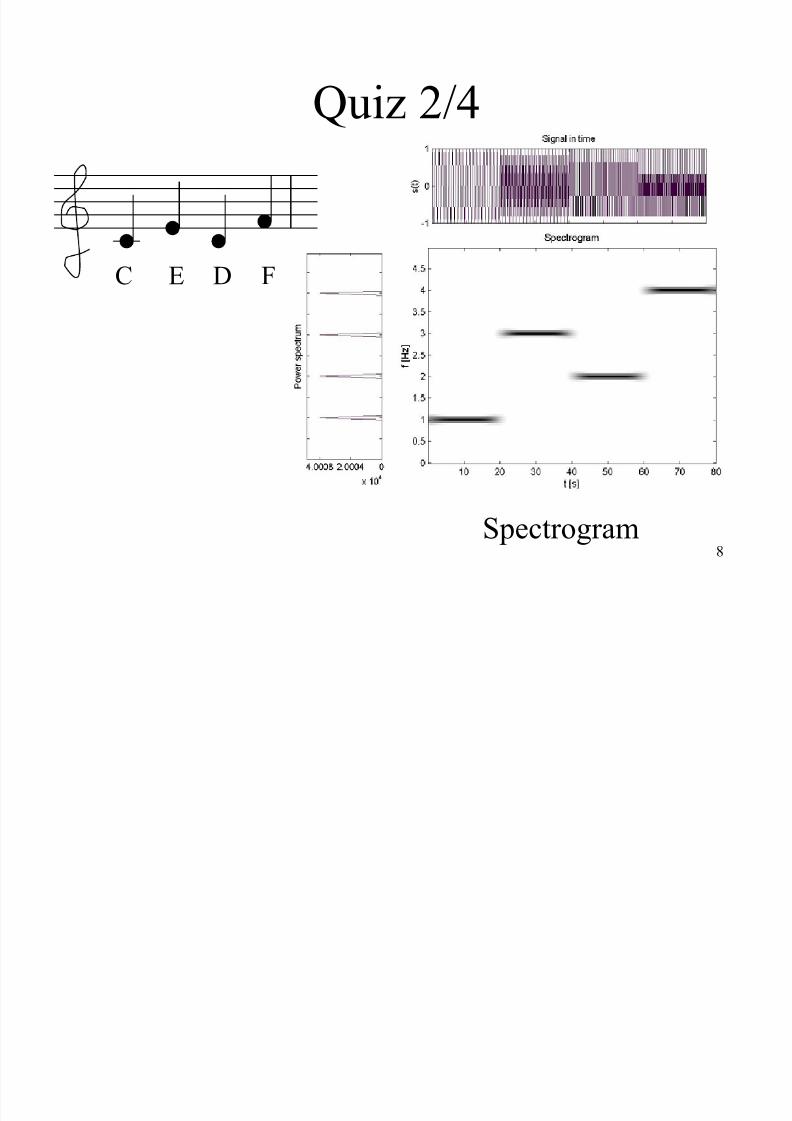
Quiz 2/4
C E D F
Spectrogram
8/14/2019 Introduction to Timefrequencyanalysis Ssp&Mm 2013-14
http://slidepdf.com/reader/full/introduction-to-timefrequencyanalysis-sspmm-2013-14 9/61
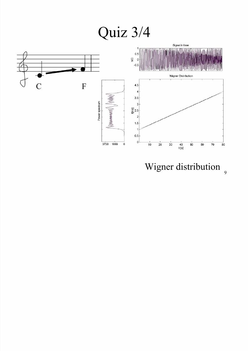
9
Quiz 3/4
C F
Wigner distribution
8/14/2019 Introduction to Timefrequencyanalysis Ssp&Mm 2013-14
http://slidepdf.com/reader/full/introduction-to-timefrequencyanalysis-sspmm-2013-14 10/61
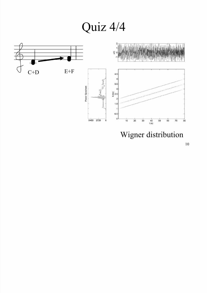
10
Quiz 4/4
C+D
Wigner distribution
E+F
8/14/2019 Introduction to Timefrequencyanalysis Ssp&Mm 2013-14
http://slidepdf.com/reader/full/introduction-to-timefrequencyanalysis-sspmm-2013-14 11/61
11
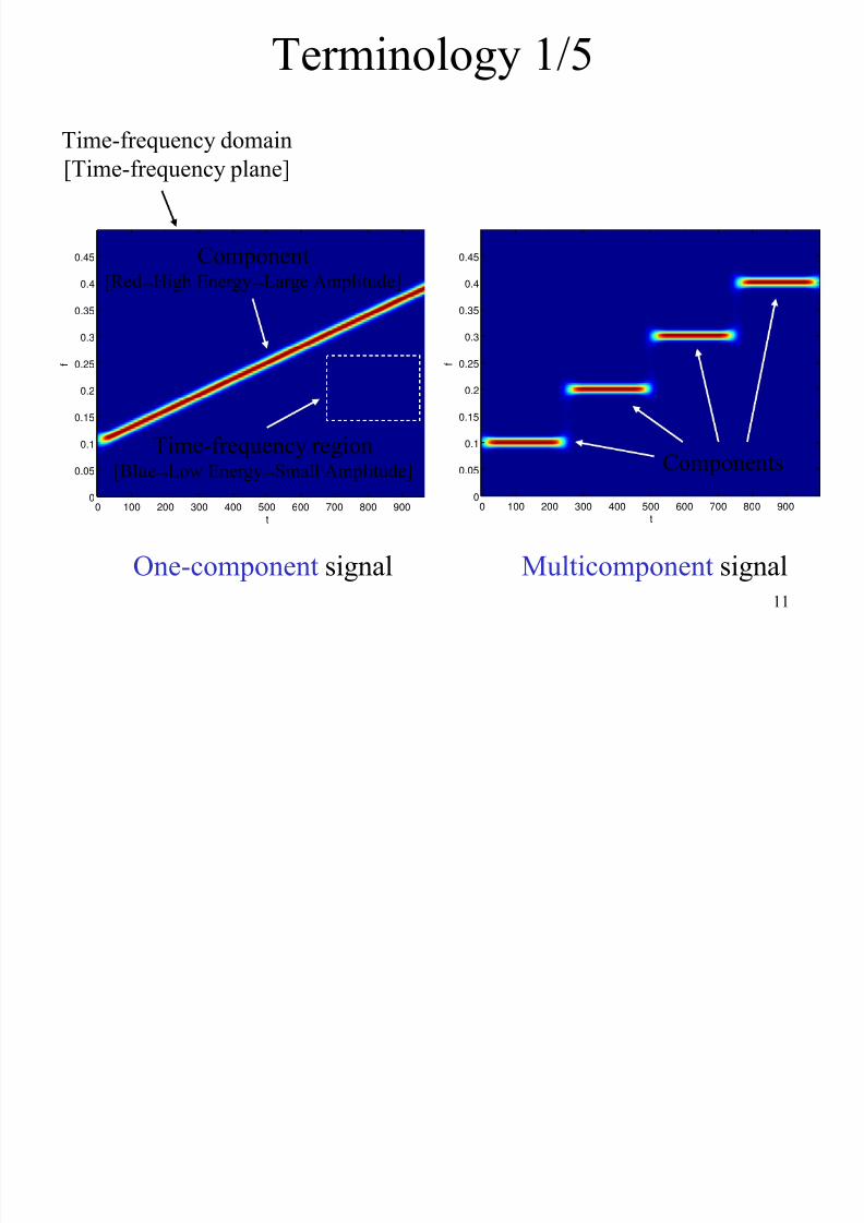
Terminology 1/5
t
f
0 100 200 300 400 500 600 700 800 9000
0.05
0.1
0.15
0.2
0.25
0.3
0.35
0.4
0.45
One-component signal
Time-frequency domain
[Time-frequency plane]
Component[Red→High Energy→Large Amplitude]
Time-frequency region[Blue→Low Energy→Small Amplitude]
t
f
0 100 200 300 400 500 600 700 800 9000
0.05
0.1
0.15
0.2
0.25
0.3
0.35
0.4
0.45
Multicomponent signal
Components
8/14/2019 Introduction to Timefrequencyanalysis Ssp&Mm 2013-14
http://slidepdf.com/reader/full/introduction-to-timefrequencyanalysis-sspmm-2013-14 12/61
12
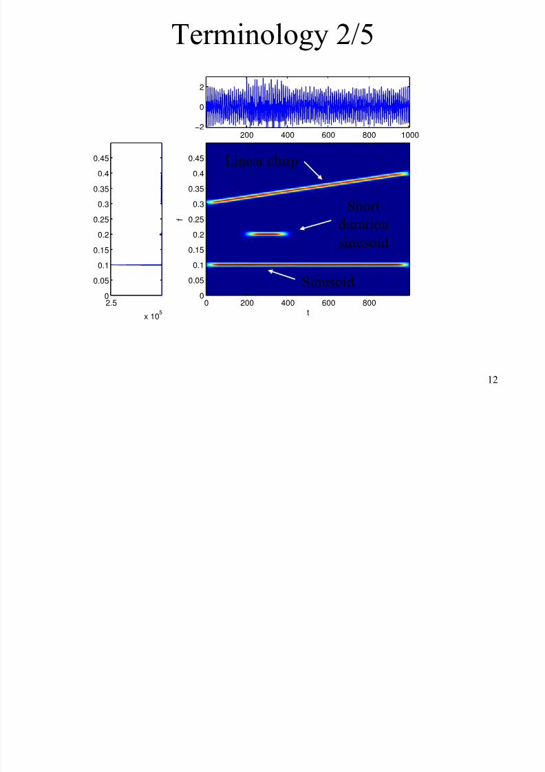
Terminology 2/5
2.5
x 105
0
0.05
0.1
0.15
0.2
0.25
0.3
0.35
0.4
0.45
200 400 600 800 1000−2
0
2
t
f
0 200 400 600 8000
0.05
0.1
0.15
0.2
0.25
0.3
0.35
0.4
0.45
Sinusoid
Short
duration
sinusoid
Linear chirp

8/14/2019 Introduction to Timefrequencyanalysis Ssp&Mm 2013-14
http://slidepdf.com/reader/full/introduction-to-timefrequencyanalysis-sspmm-2013-14 13/61
13
Terminology 3/5
10
0.050.1
0.15
0.2
0.25
0.3
0.35
0.4
0.45
200 400 600 800 10000
0.5
1
t
f
0 200 400 600 8000
0.050.1
0.15
0.2
0.25
0.3
0.35
0.4
0.45
Delta function
8/14/2019 Introduction to Timefrequencyanalysis Ssp&Mm 2013-14
http://slidepdf.com/reader/full/introduction-to-timefrequencyanalysis-sspmm-2013-14 14/61
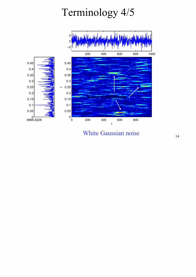
14
Terminology 4/5
6965.62260
0.05
0.1
0.15
0.2
0.25
0.3
0.35
0.4
0.45
200 400 600 800 1000
−2
0
2
t
f
0 200 400 600 8000
0.05
0.1
0.15
0.2
0.25
0.3
0.35
0.4
0.45
Noise components
White Gaussian noise
8/14/2019 Introduction to Timefrequencyanalysis Ssp&Mm 2013-14
http://slidepdf.com/reader/full/introduction-to-timefrequencyanalysis-sspmm-2013-14 15/61
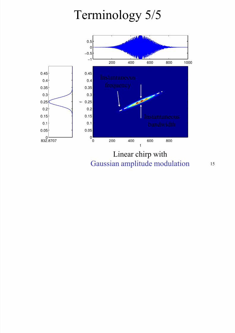
15
Terminology 5/5
832.87070
0.05
0.1
0.15
0.2
0.25
0.3
0.35
0.4
0.45
200 400 600 800 1000
−1
−0.5
0
0.5
t
f
0 200 400 600 8000
0.05
0.1
0.15
0.2
0.25
0.3
0.35
0.4
0.45
Linear chirp withGaussian amplitude modulation
Instantaneous
frequency
Instantaneous
bandwidth
8/14/2019 Introduction to Timefrequencyanalysis Ssp&Mm 2013-14
http://slidepdf.com/reader/full/introduction-to-timefrequencyanalysis-sspmm-2013-14 16/61
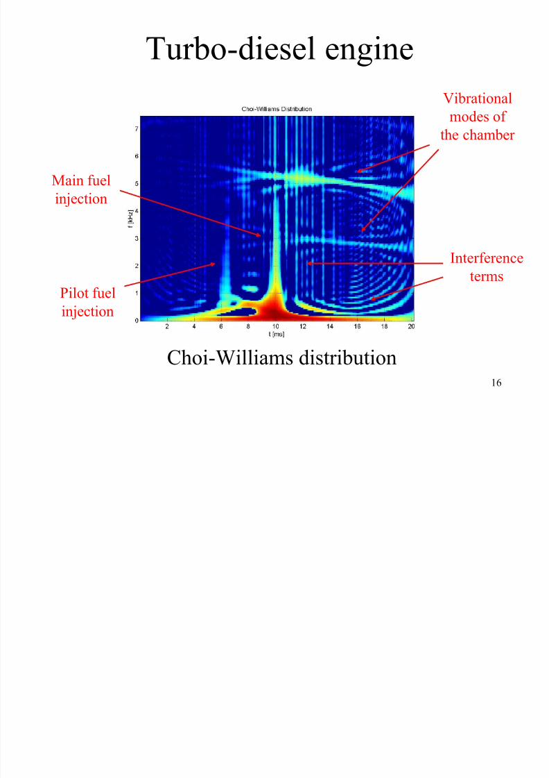
16
Turbo-diesel engine
Choi-Williams distribution
Pilot fuelinjection
Main fuel
injection
Vibrational
modes of
the chamber
Interference
terms
8/14/2019 Introduction to Timefrequencyanalysis Ssp&Mm 2013-14
http://slidepdf.com/reader/full/introduction-to-timefrequencyanalysis-sspmm-2013-14 17/61
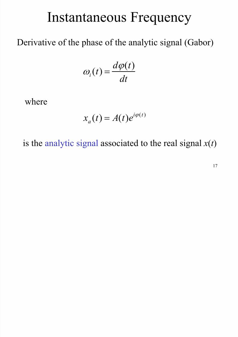
17
Instantaneous Frequency
Derivative of the phase of the analytic signal (Gabor)
dt
t d t i
)()( ϕ ω =
where
)()()( t i
a et At x ϕ =
is the analytic signal associated to the real signal x(t )
8/14/2019 Introduction to Timefrequencyanalysis Ssp&Mm 2013-14
http://slidepdf.com/reader/full/introduction-to-timefrequencyanalysis-sspmm-2013-14 18/61
18
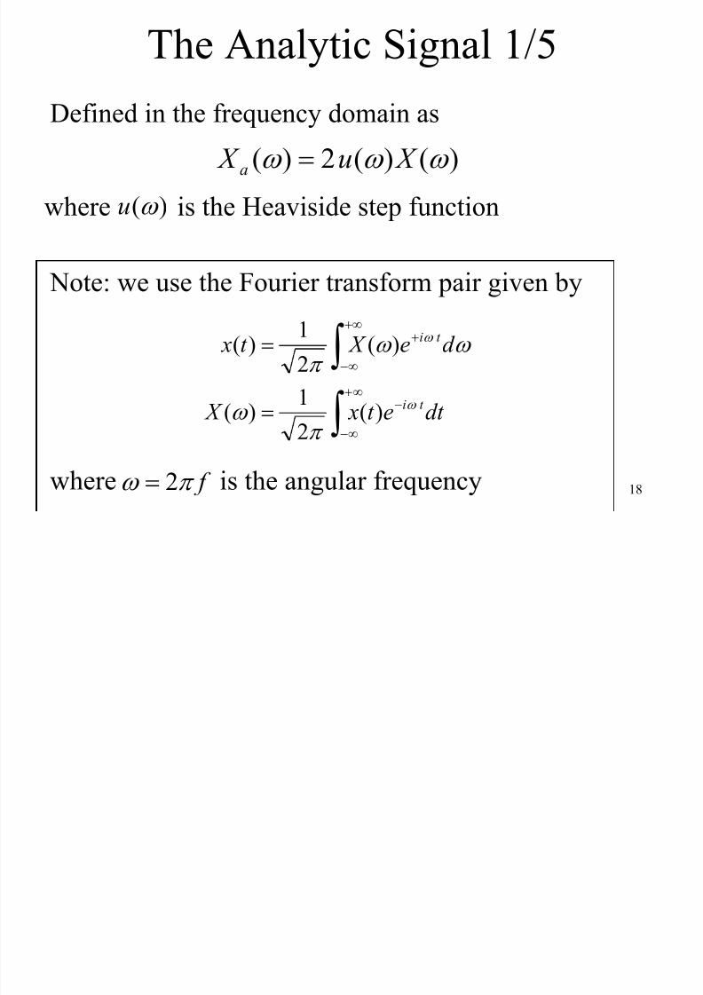
The Analytic Signal 1/5
Defined in the frequency domain as
)()(2)( ω ω ω X u X a =
∫
∫∞+
∞−
−
+∞
∞−
+
=
=
dt et x X
d e X t x
t i
t i
ω
ω
π ω
ω ω
π
)(2
1)(
)(
2
1)(
Note: we use the Fourier transform pair given by
where f π ω 2= is the angular frequency
where )(ω u is the Heaviside step function
8/14/2019 Introduction to Timefrequencyanalysis Ssp&Mm 2013-14
http://slidepdf.com/reader/full/introduction-to-timefrequencyanalysis-sspmm-2013-14 19/61
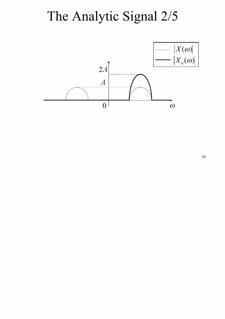
19
The Analytic Signal 2/5
ω 0
)(ω X
)(ω a X 2
8/14/2019 Introduction to Timefrequencyanalysis Ssp&Mm 2013-14
http://slidepdf.com/reader/full/introduction-to-timefrequencyanalysis-sspmm-2013-14 20/61
20
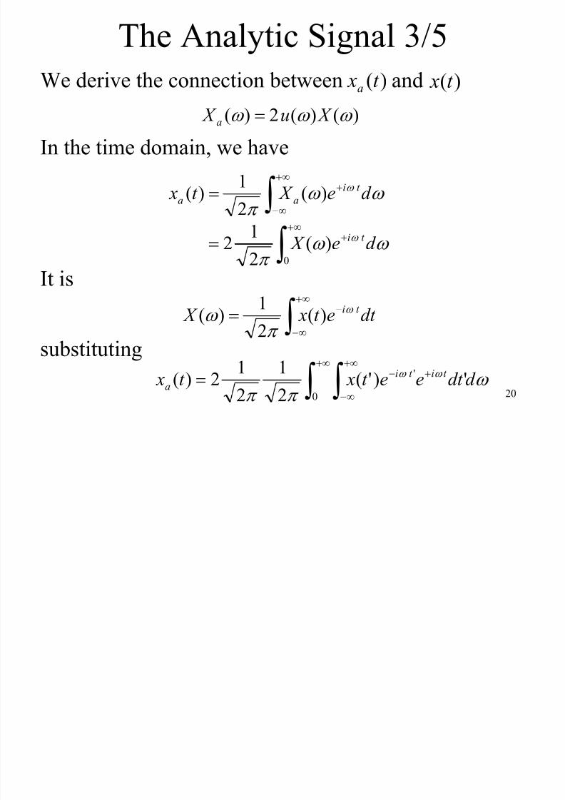
The Analytic Signal 3/5
We derive the connection between )(t xa and )(t x
∫+∞
∞−
+= ω ω π
ω d e X t x t i
aa )(2
1)(
)()(2)( ω ω ω X u X a =
In the time domain, we have
It is
∫+∞
∞−
−= dt et x X t iω
π ω )(
2
1)(
substituting
∫ ∫+∞ +∞
∞−
+−=0
' ')'(21
212)( ω
π π ω ω d dt eet xt x t it i
a
∫+∞
+=0
)(2
12 ω ω
π
ω d e X t i

8/14/2019 Introduction to Timefrequencyanalysis Ssp&Mm 2013-14
http://slidepdf.com/reader/full/introduction-to-timefrequencyanalysis-sspmm-2013-14 21/61
21
The Analytic Signal 4/5
∫ ∫+∞ +∞
∞−
−+=0
)'( ')'(1
)( ω π
ω d dt et xt x t t i
a
We now consider the identity
z
i z d e z i +=∫
+∞
)(0
πδ ω ω
By setting
∫
+∞
∞− ⎥
⎦
⎤⎢⎣
⎡
−
+−= '
'
)'()'(1
)( dt
t t
it t t xt xa πδ
π
't t z −= it is
)(t x
∫∫ +∞
∞−
+∞
∞− −+−= '
'
)'(')'()'( dt
t t
t xidt t t t x
π δ

8/14/2019 Introduction to Timefrequencyanalysis Ssp&Mm 2013-14
http://slidepdf.com/reader/full/introduction-to-timefrequencyanalysis-sspmm-2013-14 22/61
22
The Analytic Signal 5/5
∫+∞
∞− −+= '
'
)'()()( dt
t t
t xit xt xa
π
We note that
{ } )()( t xt xa =ℜ
which is the reason for the “2” in the definition of theanalytic signal
Hilbert transform of )(t x
8/14/2019 Introduction to Timefrequencyanalysis Ssp&Mm 2013-14
http://slidepdf.com/reader/full/introduction-to-timefrequencyanalysis-sspmm-2013-14 23/61
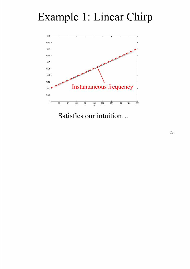
23
Example 1: Linear Chirp
Satisfies our intuition…
Instantaneous frequency
E l 2 S f T Li Chi !
8/14/2019 Introduction to Timefrequencyanalysis Ssp&Mm 2013-14
http://slidepdf.com/reader/full/introduction-to-timefrequencyanalysis-sspmm-2013-14 24/61
24
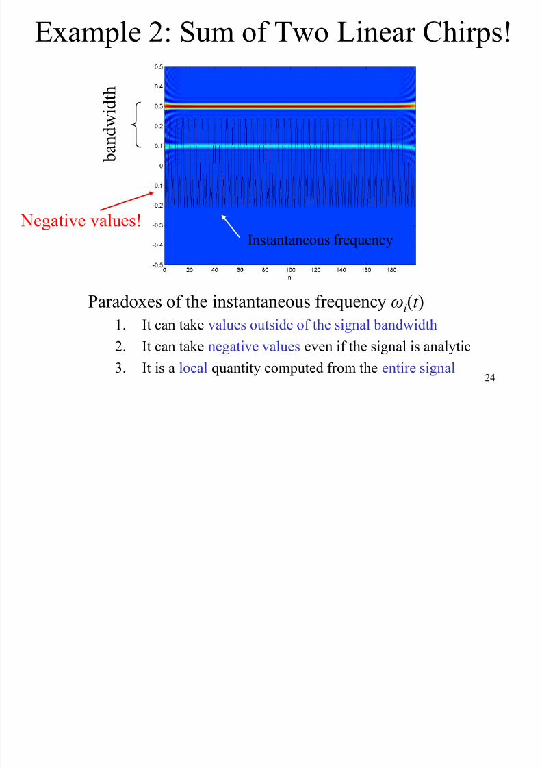
Example 2: Sum of Two Linear Chirps!
Instantaneous frequency
Paradoxes of the instantaneous frequency ωi(t )
1. It can take values outside of the signal bandwidth
2. It can take negative values even if the signal is analytic
3. It is a local quantity computed from the entire signal
b a n d w i d t h
Negative values!
8/14/2019 Introduction to Timefrequencyanalysis Ssp&Mm 2013-14
http://slidepdf.com/reader/full/introduction-to-timefrequencyanalysis-sspmm-2013-14 25/61
25
Abundance of TF distributions
There are infinite Time-Frequency Distributions• Spectrogram
• Wigner distribution (or Wigner-Ville)
• Cohen’s class
– Smoothed Pseudo-Wigner
– Choi-Williams
8/14/2019 Introduction to Timefrequencyanalysis Ssp&Mm 2013-14
http://slidepdf.com/reader/full/introduction-to-timefrequencyanalysis-sspmm-2013-14 26/61
26
Cohen’s class
• 1966: Journal of Mathematical Physics• It collects all TF distributions
• Every TFD has a kernel
• A new TFD can be designed by imposing someconstraints of the kernel
θ τ τ θ φ τ τ π ω θ τω θτ
∫∫∫ +−−
+−= d dud eu xu xt C uiii
),()2/()2/(*4
1
),( 2

8/14/2019 Introduction to Timefrequencyanalysis Ssp&Mm 2013-14
http://slidepdf.com/reader/full/introduction-to-timefrequencyanalysis-sspmm-2013-14 27/61
27
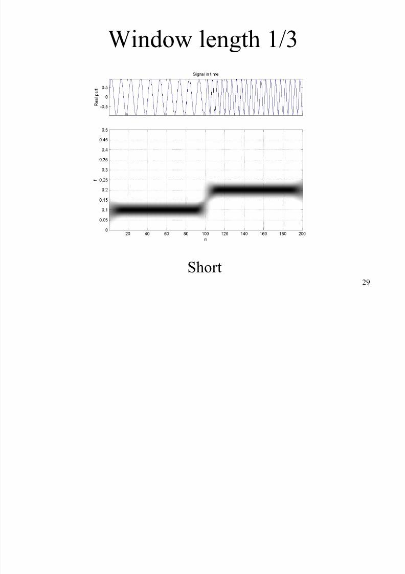
Spectrogram
• Most intuitive TF distribution
• h(t ) is the window
• h(t -τ ) x(τ ) is the windowed signal
• Squared magnitude of the Short Time Fourier
Transform (STFT)
2
d)()(2
1),( ∫
∞+
∞−
−−= τ τ τ π
ω ω τ ie xt ht P
8/14/2019 Introduction to Timefrequencyanalysis Ssp&Mm 2013-14
http://slidepdf.com/reader/full/introduction-to-timefrequencyanalysis-sspmm-2013-14 28/61
28
Positivity and Marginals
1.
2. Marginals are not satisfied
2)(),( ω ω X dt t P ≠∫2
)(),( t xd t P ≠∫ ω ω
0),( ≥ω t P
8/14/2019 Introduction to Timefrequencyanalysis Ssp&Mm 2013-14
http://slidepdf.com/reader/full/introduction-to-timefrequencyanalysis-sspmm-2013-14 29/61
29
Window length 1/3
Short
8/14/2019 Introduction to Timefrequencyanalysis Ssp&Mm 2013-14
http://slidepdf.com/reader/full/introduction-to-timefrequencyanalysis-sspmm-2013-14 30/61
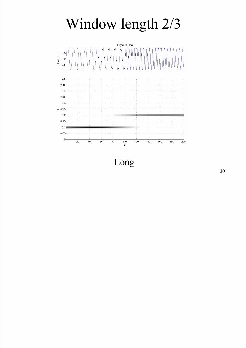
30
Window length 2/3
Long

8/14/2019 Introduction to Timefrequencyanalysis Ssp&Mm 2013-14
http://slidepdf.com/reader/full/introduction-to-timefrequencyanalysis-sspmm-2013-14 31/61
31
Window length 3/3
Medium
8/14/2019 Introduction to Timefrequencyanalysis Ssp&Mm 2013-14
http://slidepdf.com/reader/full/introduction-to-timefrequencyanalysis-sspmm-2013-14 32/61
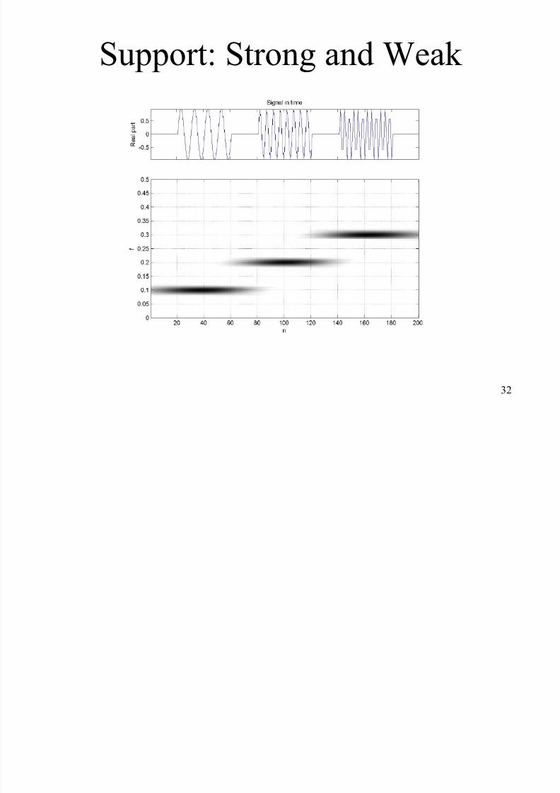
32
Support: Strong and Weak
8/14/2019 Introduction to Timefrequencyanalysis Ssp&Mm 2013-14
http://slidepdf.com/reader/full/introduction-to-timefrequencyanalysis-sspmm-2013-14 33/61
33
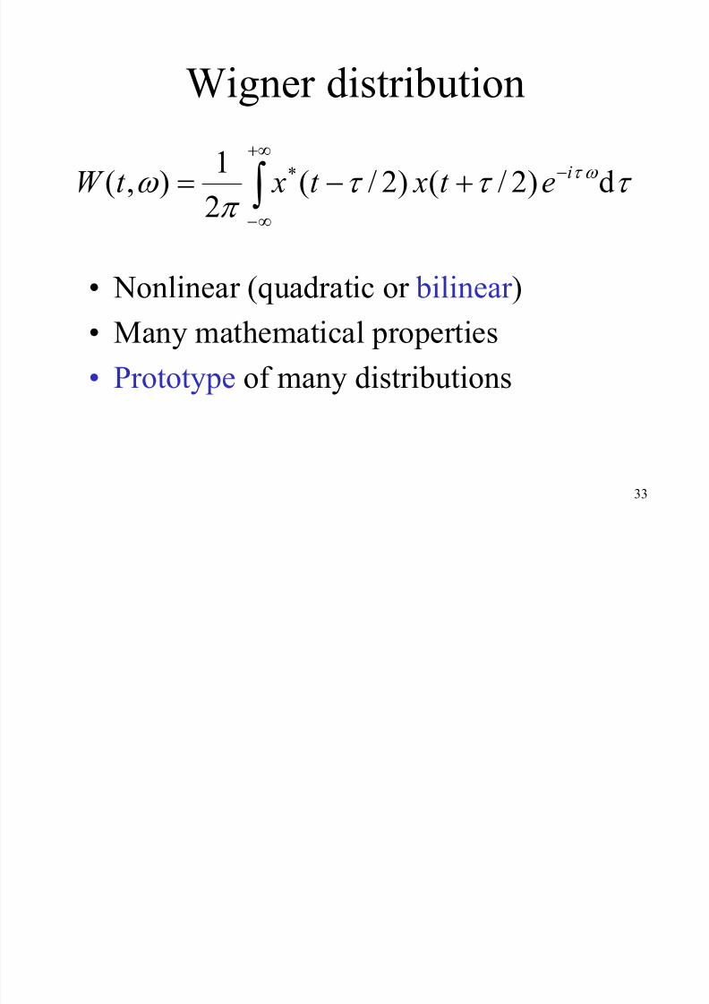
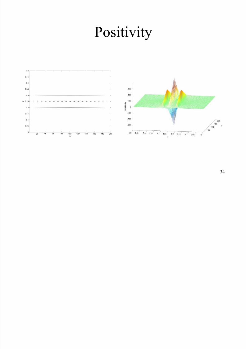
Wigner distribution
∫
+∞
∞−
−
+−= τ τ τ π ω
ω τ
d)2/()2/(2
1
),(* i
et xt xt W
• Nonlinear (quadratic or bilinear )• Many mathematical properties
• Prototype of many distributions
8/14/2019 Introduction to Timefrequencyanalysis Ssp&Mm 2013-14
http://slidepdf.com/reader/full/introduction-to-timefrequencyanalysis-sspmm-2013-14 34/61
34
Positivity
8/14/2019 Introduction to Timefrequencyanalysis Ssp&Mm 2013-14
http://slidepdf.com/reader/full/introduction-to-timefrequencyanalysis-sspmm-2013-14 35/61
35
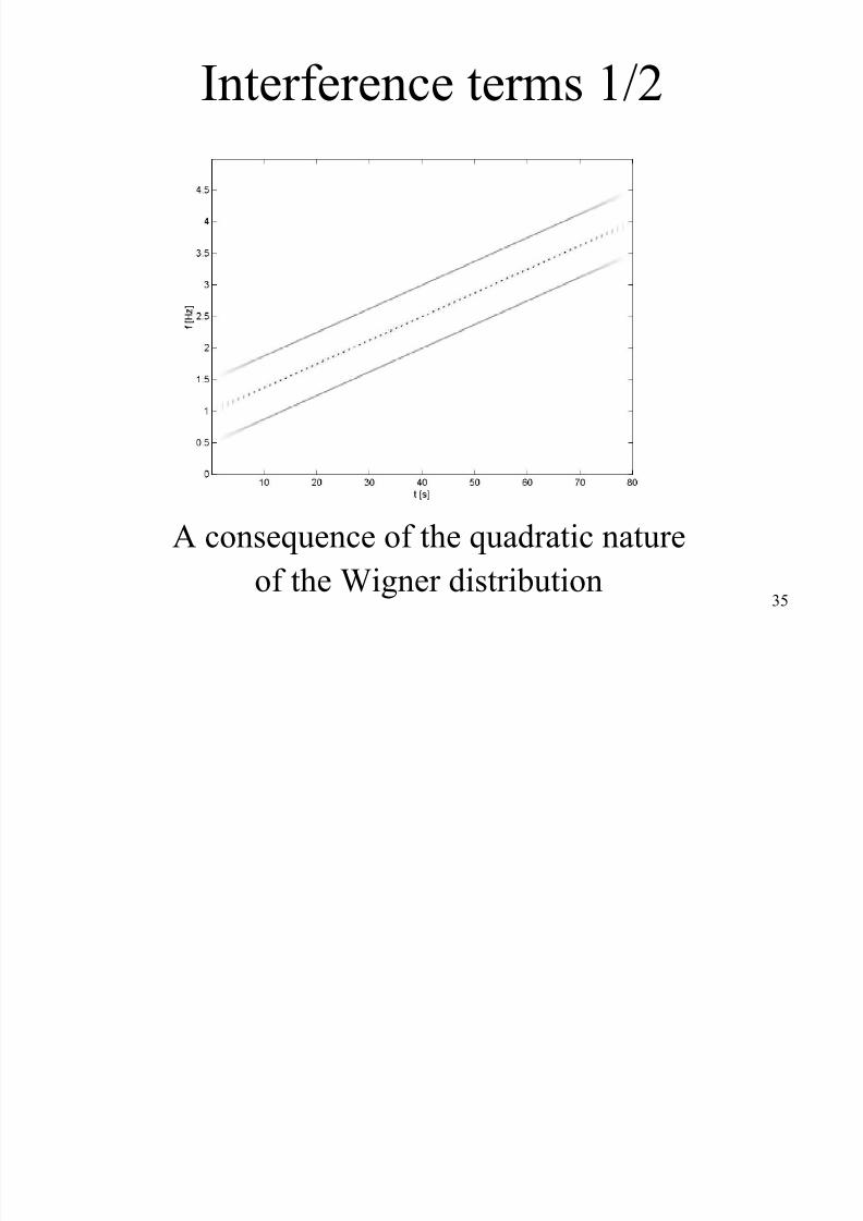
Interference terms 1/2
A consequence of the quadratic nature
of the Wigner distribution
8/14/2019 Introduction to Timefrequencyanalysis Ssp&Mm 2013-14
http://slidepdf.com/reader/full/introduction-to-timefrequencyanalysis-sspmm-2013-14 36/61
36
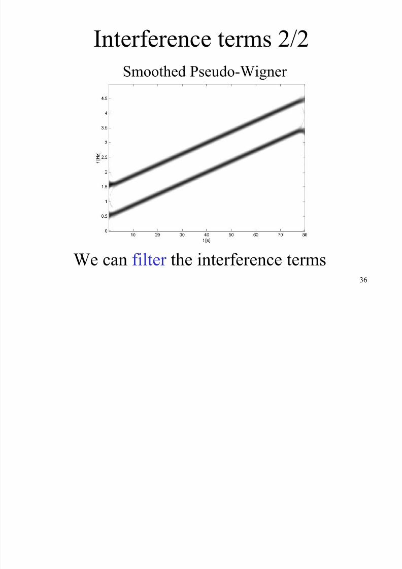
Interference terms 2/2
We can filter the interference terms
Smoothed Pseudo-Wigner
8/14/2019 Introduction to Timefrequencyanalysis Ssp&Mm 2013-14
http://slidepdf.com/reader/full/introduction-to-timefrequencyanalysis-sspmm-2013-14 37/61
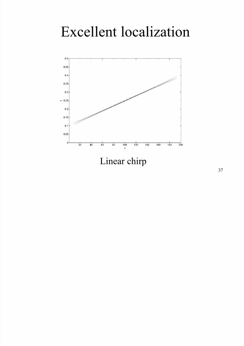
37
Excellent localization
Linear chirp

8/14/2019 Introduction to Timefrequencyanalysis Ssp&Mm 2013-14
http://slidepdf.com/reader/full/introduction-to-timefrequencyanalysis-sspmm-2013-14 38/61
38
Support: Strong and Weak
8/14/2019 Introduction to Timefrequencyanalysis Ssp&Mm 2013-14
http://slidepdf.com/reader/full/introduction-to-timefrequencyanalysis-sspmm-2013-14 39/61
39
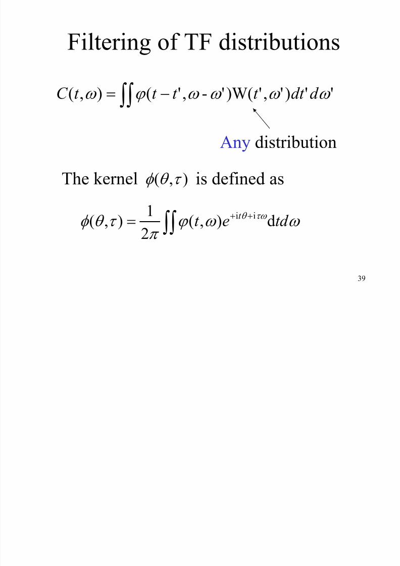
Filtering of TF distributions
∫∫ −= '')',')W('-,'(),( ω ω ω ω ϕ ω d dt t t t t C
Any distribution
∫∫ ++= ω ω ϕ
π τ θ φ τω θ td et t d),(
21),( ii
The kernel is defined as),( τ θ φ
8/14/2019 Introduction to Timefrequencyanalysis Ssp&Mm 2013-14
http://slidepdf.com/reader/full/introduction-to-timefrequencyanalysis-sspmm-2013-14 40/61
40
Constraints on the kernel
• Positivity
• Time and frequency marginals
• Interference terms
• Strong and weak support
• Instantaneous frequency
• ...
8/14/2019 Introduction to Timefrequencyanalysis Ssp&Mm 2013-14
http://slidepdf.com/reader/full/introduction-to-timefrequencyanalysis-sspmm-2013-14 41/61
41
TFA of random processes
• Very young field
– Wigner spectrum
– Sliding Welch spectrum
Wi S
8/14/2019 Introduction to Timefrequencyanalysis Ssp&Mm 2013-14
http://slidepdf.com/reader/full/introduction-to-timefrequencyanalysis-sspmm-2013-14 42/61
42
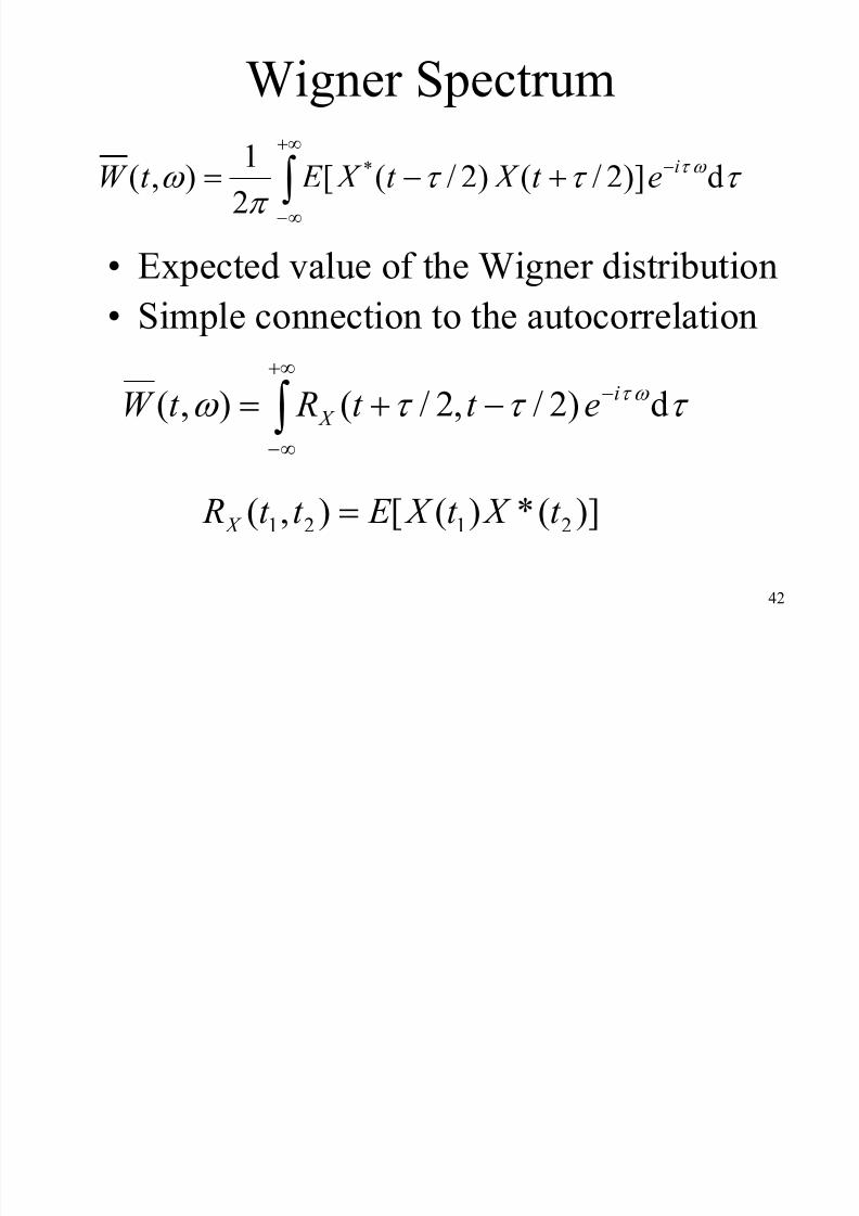
Wigner Spectrum
∫+∞
∞−
−+−= τ τ τ π
ω ω τ d)]2/()2/([2
1),( * iet X t X E t W
• Expected value of the Wigner distribution
• Simple connection to the autocorrelation
∫+∞
∞−
−−+= τ τ τ ω ω τ d)2/,2/(),( i
X et t Rt W
)](*)([),( 2121 t X t X E t t R X =
Sliding Welch spectrum
8/14/2019 Introduction to Timefrequencyanalysis Ssp&Mm 2013-14
http://slidepdf.com/reader/full/introduction-to-timefrequencyanalysis-sspmm-2013-14 43/61
4343
Sliding Welch spectrum
Almost identical to the spectrogram:
rather than computing the squared FFT ofthe truncated signal (basic periodogram), we
evaluate its Welch periodogram
A li i
8/14/2019 Introduction to Timefrequencyanalysis Ssp&Mm 2013-14
http://slidepdf.com/reader/full/introduction-to-timefrequencyanalysis-sspmm-2013-14 44/61
44
Applications
• Time-frequency representation of dynamical
systems
– Deterministic case
– Random case• Quasi-Periodic Oscillations in a binary star
The Study of Dynamical Systems
8/14/2019 Introduction to Timefrequencyanalysis Ssp&Mm 2013-14
http://slidepdf.com/reader/full/introduction-to-timefrequencyanalysis-sspmm-2013-14 45/61
45
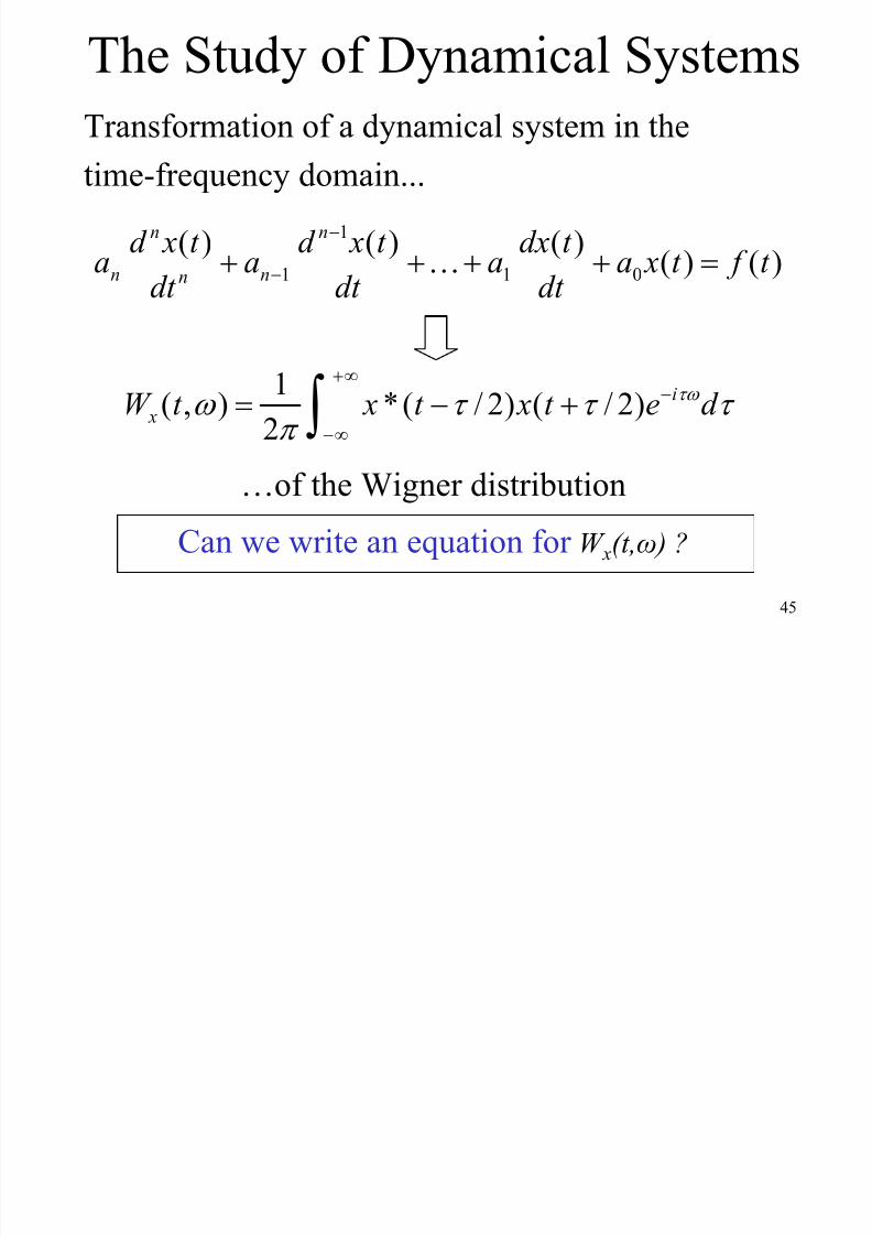
The Study of Dynamical Systems
Transformation of a dynamical system in thetime-frequency domain...
)()()()()(01
1
1 t f t xadt
t dxadt
t xd adt
t xd an
nn
n
n =++++−
− K
…of the Wigner distribution
Can we write an equation for W x(t,ω ) ?
∫ ∞+
∞−
−+−= τ τ τ π
ω τω d et xt xt W i
x )2/()2/(*2
1),(
h i i h f
8/14/2019 Introduction to Timefrequencyanalysis Ssp&Mm 2013-14
http://slidepdf.com/reader/full/introduction-to-timefrequencyanalysis-sspmm-2013-14 46/61
46
Why it is worth to transform
1. Better understanding of the system behavior
2. New system identification methods
3. New system design methods
8/14/2019 Introduction to Timefrequencyanalysis Ssp&Mm 2013-14
http://slidepdf.com/reader/full/introduction-to-timefrequencyanalysis-sspmm-2013-14 47/61
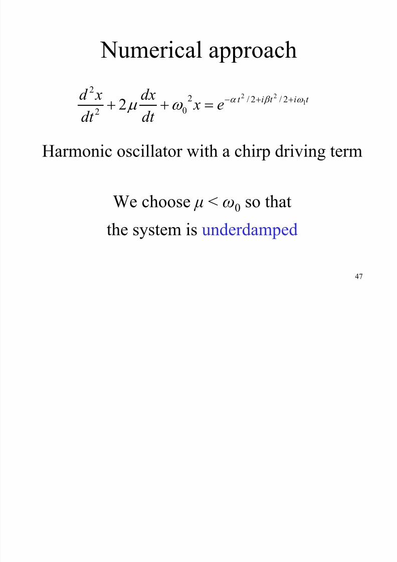
47
Numerical approach
Harmonic oscillator with a chirp driving term
We choose μ < ω0
so that
the system is underdamped
t it it
e xdt
dx
dt
xd 1
22 2/2/2
02
2
2
ω β α
ω μ
++−
=++
8/14/2019 Introduction to Timefrequencyanalysis Ssp&Mm 2013-14
http://slidepdf.com/reader/full/introduction-to-timefrequencyanalysis-sspmm-2013-14 48/61
48
−8 −6 −4 −2 0 2 4 6 8 10
−2
−1.5
−1
−0.5
0
0.5
1
1.5
2
x 10−3
t (s)
x ( t )
−10 −8 −6 −4 −2 0 2 4 6 8 10 12
10−7
10−6
10−5
10−4
10−3
f (Hz)
| X ( f ) | 2
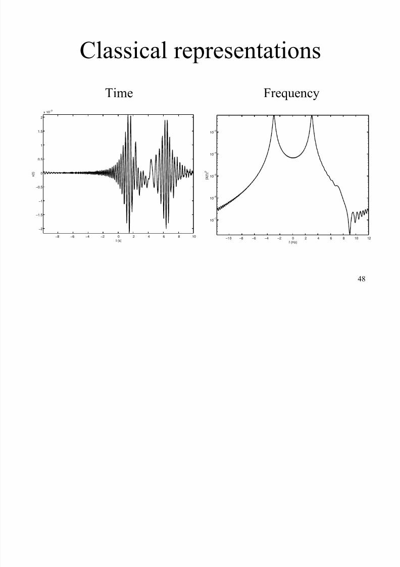
Time Frequency
Classical representations

8/14/2019 Introduction to Timefrequencyanalysis Ssp&Mm 2013-14
http://slidepdf.com/reader/full/introduction-to-timefrequencyanalysis-sspmm-2013-14 49/61
49
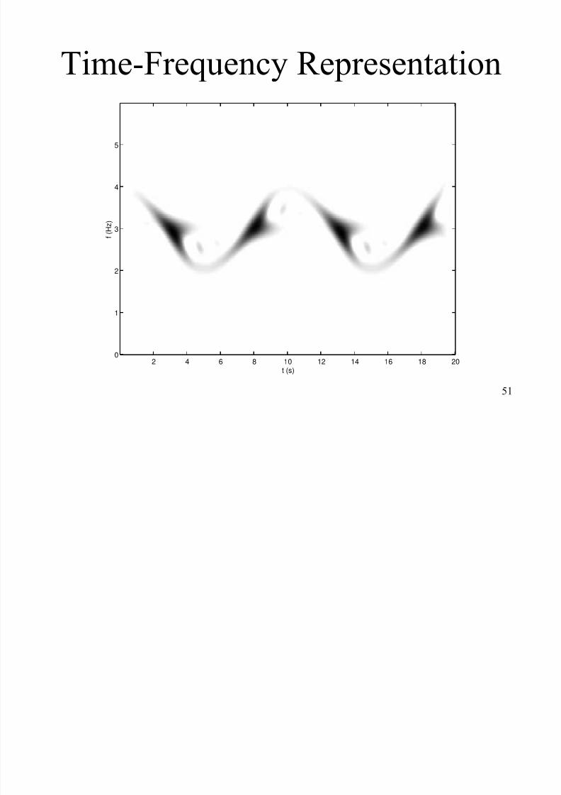
Time-Frequency Representation
t (s)
f ( H z )
1 2 3 4 5 6 7 8 9 100
1
2
3
4
5
t
f
Sinusoidal FM chirp

8/14/2019 Introduction to Timefrequencyanalysis Ssp&Mm 2013-14
http://slidepdf.com/reader/full/introduction-to-timefrequencyanalysis-sspmm-2013-14 50/61
50
p
t it ie x
dt
dx
dt
xd 21 sin2
02
2
2 ω α ω
ω μ +=++
0 2 4 6 8 10 12 14 16 18
−0.015
−0.01
−0.005
0
0.005
0.01
0.015
t (s)
x ( t )
0 1 2 3 4 5 6
10−5
10−4
10
−3
10−2
10−1
100
f (Hz)
| X ( f ) | 2
Time Frequency
3 f [Hz]
i i
8/14/2019 Introduction to Timefrequencyanalysis Ssp&Mm 2013-14
http://slidepdf.com/reader/full/introduction-to-timefrequencyanalysis-sspmm-2013-14 51/61
51
Time-Frequency Representation
t (s)
f ( H
z )
2 4 6 8 10 12 14 16 18 200
1
2
3
4
5
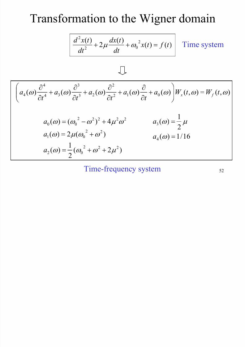
Transformation to the Wigner domain
8/14/2019 Introduction to Timefrequencyanalysis Ssp&Mm 2013-14
http://slidepdf.com/reader/full/introduction-to-timefrequencyanalysis-sspmm-2013-14 52/61
52
g
)()()(
2)( 2
02
2
t f t xdt
t dx
dt
t xd =++ ω μ
)2(2
1)(
)(2)(
4)()(
222
02
2201
22222
00
μ ω ω ω
ω ω μ ω
ω μ ω ω ω
++=
+=
+−=
a
a
a
),(),()()()()()( 012
2
23
3
34
4
4 ω ω ω ω ω ω ω t W t W a
t
a
t
a
t
a
t
a f x =⎟⎟
⎠
⎞⎜⎜
⎝
⎛ +
∂
∂+
∂
∂+
∂
∂+
∂
∂
16/1)(
2
1)(
4
3
=
=
ω
μ ω
a
a
Time system
Time-frequency system
Impulse response
8/14/2019 Introduction to Timefrequencyanalysis Ssp&Mm 2013-14
http://slidepdf.com/reader/full/introduction-to-timefrequencyanalysis-sspmm-2013-14 53/61
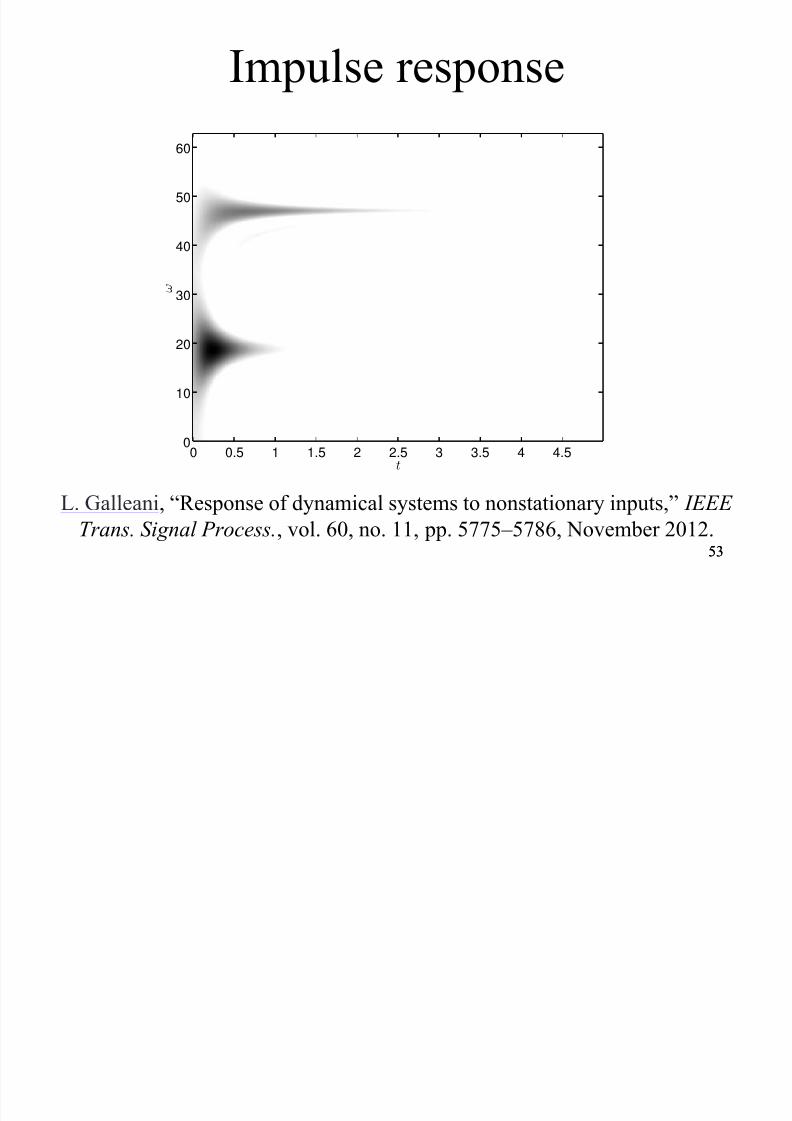
5353
t
ω
0 0.5 1 1.5 2 2.5 3 3.5 4 4.50
10
20
30
40
50
60
Impulse response
L. Galleani, “Response of dynamical systems to nonstationary inputs,” IEEE
Trans. Signal Process., vol. 60, no. 11, pp. 5775–5786, November 2012.
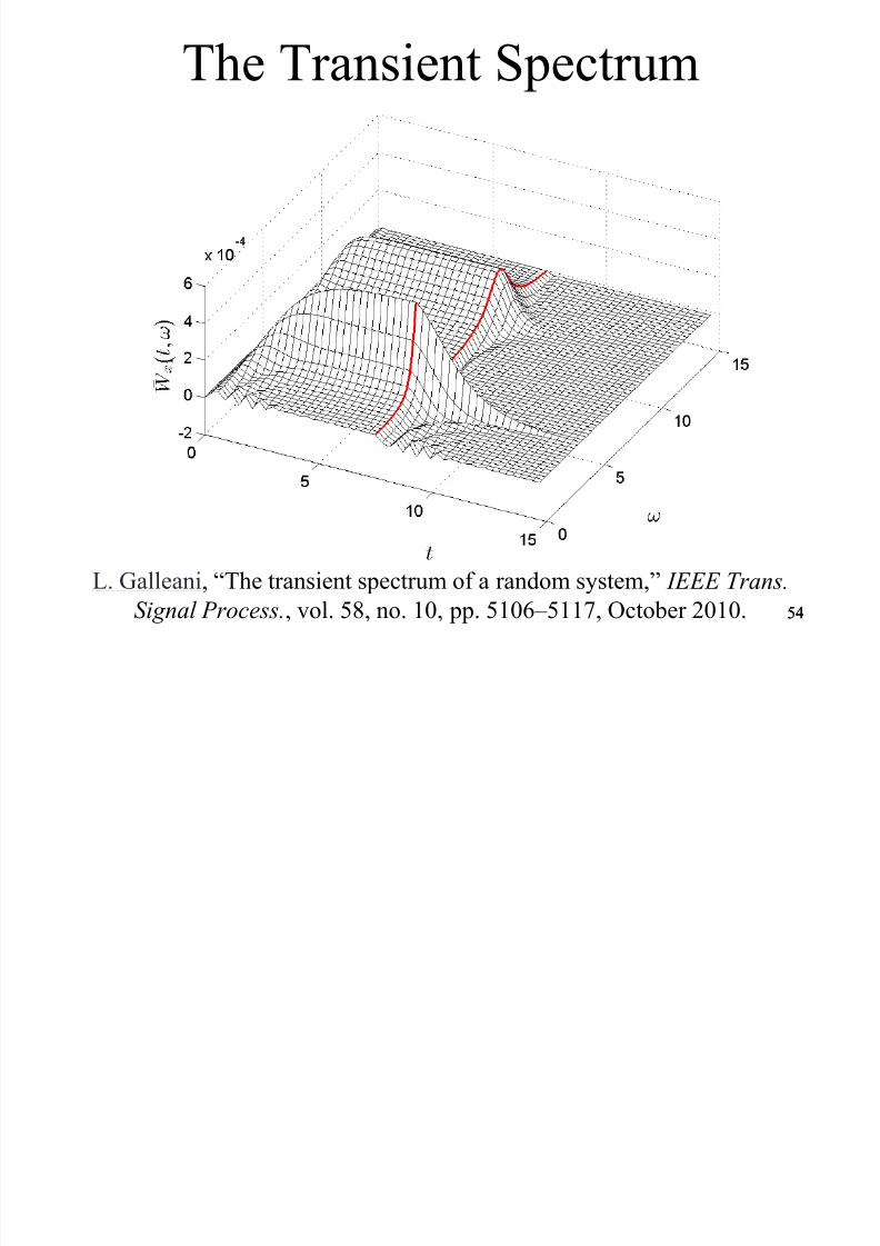
The Transient Spectrum
8/14/2019 Introduction to Timefrequencyanalysis Ssp&Mm 2013-14
http://slidepdf.com/reader/full/introduction-to-timefrequencyanalysis-sspmm-2013-14 54/61
5454
p
L. Galleani, “The transient spectrum of a random system,” IEEE Trans.Signal Process., vol. 58, no. 10, pp. 5106–5117, October 2010.
Sliding Welch Spectrum 1/3

8/14/2019 Introduction to Timefrequencyanalysis Ssp&Mm 2013-14
http://slidepdf.com/reader/full/introduction-to-timefrequencyanalysis-sspmm-2013-14 55/61
55
Sliding Welch Spectrum 1/3
X-Ray binary star
Sliding Welch Spectrum 2/3
8/14/2019 Introduction to Timefrequencyanalysis Ssp&Mm 2013-14
http://slidepdf.com/reader/full/introduction-to-timefrequencyanalysis-sspmm-2013-14 56/61
56
Sliding Welch Spectrum 2/3
Measured signal: photon arrival time
0
0.10.12
0.15...
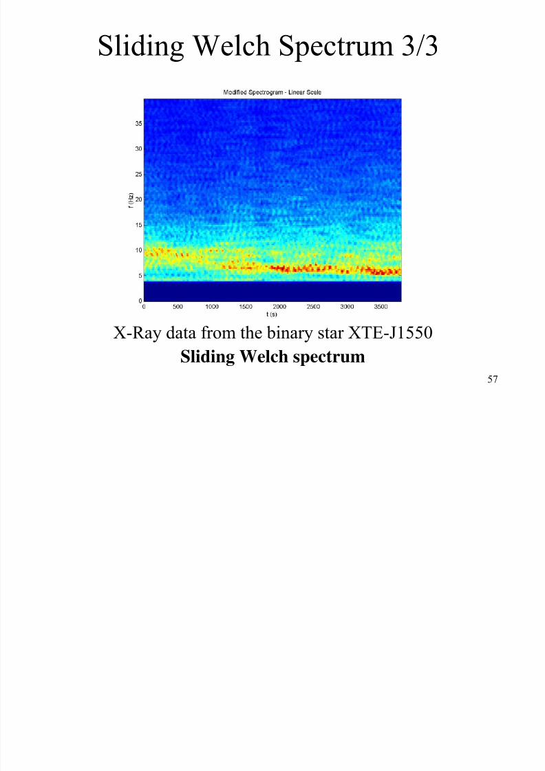
Sliding Welch Spectrum 3/3
8/14/2019 Introduction to Timefrequencyanalysis Ssp&Mm 2013-14
http://slidepdf.com/reader/full/introduction-to-timefrequencyanalysis-sspmm-2013-14 57/61
57
g p
X-Ray data from the binary star XTE-J1550
Sliding Welch spectrum
8/14/2019 Introduction to Timefrequencyanalysis Ssp&Mm 2013-14
http://slidepdf.com/reader/full/introduction-to-timefrequencyanalysis-sspmm-2013-14 58/61
58
8/14/2019 Introduction to Timefrequencyanalysis Ssp&Mm 2013-14
http://slidepdf.com/reader/full/introduction-to-timefrequencyanalysis-sspmm-2013-14 59/61
59
8/14/2019 Introduction to Timefrequencyanalysis Ssp&Mm 2013-14
http://slidepdf.com/reader/full/introduction-to-timefrequencyanalysis-sspmm-2013-14 60/61
60
Conclusions
8/14/2019 Introduction to Timefrequencyanalysis Ssp&Mm 2013-14
http://slidepdf.com/reader/full/introduction-to-timefrequencyanalysis-sspmm-2013-14 61/61
61
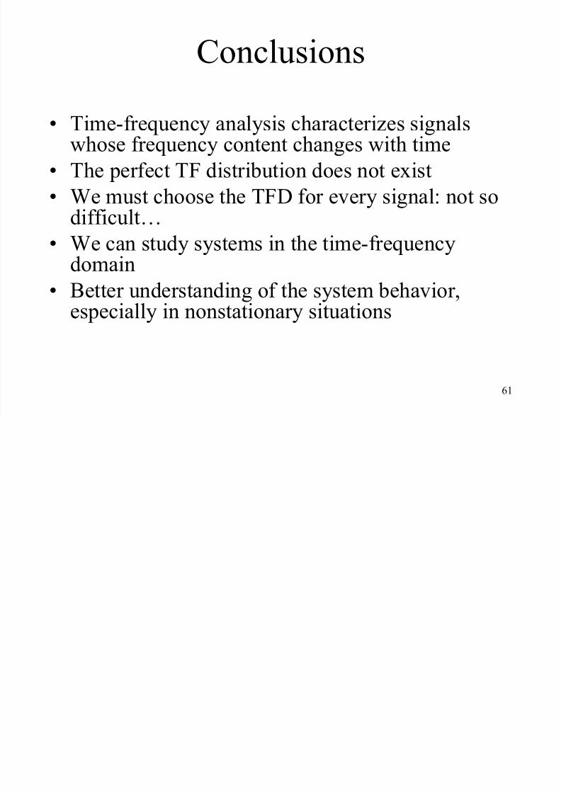
Conclusions
• Time-frequency analysis characterizes signalswhose frequency content changes with time
• The perfect TF distribution does not exist
• We must choose the TFD for every signal: not sodifficult…
• We can study systems in the time-frequencydomain
• Better understanding of the system behavior,especially in nonstationary situations