INTRODUCTION TO THE TWOPAS ASSISTANT

Final Report ITD Research Project 169

KLK252 N05-08

National Institute for Advanced Transportation Technology University of Idaho

for the Idaho Transportation Department

Michael Dixon, PhD, PE

February 2005

1-2

Table of Contents 1 Starting TWOPAS ASSISTANT ................................................................................. 1-3

1.1 Introduction to Projects and Scenarios ........................................................................ 1-3

1.2 Organization of TWOPAS ASSISTANT .................................................................... 1-3

2 Using TWOPAS ASSISTANT to Create and Run TWOPAS Simulation .................. 2-5

2.1 Run Setup ..................................................................................................................... 2-5

2.1.1 Random number seeds ................................................................................................. 2-5

2.1.2 Run time ....................................................................................................................... 2-6

2.2 Roadway Geometry ..................................................................................................... 2-7

2.2.1 General tab settings ...................................................................................................... 2-7

2.2.2 Remaining roadway geometry tabs .............................................................................. 2-8

2.2.2.1 Horizontal curves ......................................................................................................... 2-8

2.2.2.2 Vertical curves ............................................................................................................. 2-8

2.2.2.3 Sight Distance .............................................................................................................. 2-9

2.2.2.4 Pass Zones/Lanes ....................................................................................................... 2-10

2.2.2.5 Lane and shoulder width ............................................................................................ 2-11

2.2.2.6 Crawl Regions ............................................................................................................ 2-11

2.2.2.7 Reduced Speed Zone.................................................................................................. 2-12

2.3 Traffic Settings........................................................................................................... 2-13

2.4 Traffic Volume........................................................................................................... 2-14

2.5 Station Location ......................................................................................................... 2-14

2.5.1 Station Generation ..................................................................................................... 2-15

2.5.2 Station Addition ......................................................................................................... 2-15

2.5.3 Station Subsections .................................................................................................... 2-16

2.6 Create the Input File and Run TWOPAS ................................................................... 2-17

3 Viewing and Reading the Summary Output File ....................................................... 3-19

4 The TWOPAS Output Processor ............................................................................... 4-21

4.1 Open the summary files ............................................................................................. 4-22

4.2 Organize Summary Files............................................................................................ 4-23

4.3 Read in Summary Files .............................................................................................. 4-23

4.4 View Summary Data .................................................................................................. 4-23

4.5 View Station Data ...................................................................................................... 4-24

1-3

1 Starting TWOPAS ASSISTANT After double clicking on the TWOPAS ASSISTANT executable file the Project_Scenario

window will appear. TWOPAS ASSISTANT is integrated with an Access database file that will

help keep all two-lane highway projects organized. For instance, one project for US 12 could be

created and then each alternative for that project could be its own scenario.

Keep in mind that the TWOPAS ASSISTANT program does not model two-lane highways.

TWOPAS ASSISTANT helps the user create input files for the TWOPAS program, run the

TWOPAS program and view the simulation results output from TWOPAS. So, in summary

TWOPAS is the model and TWOPAS ASSISTANT just makes it easier to work with TWOPAS

by generating input data files and processing output data.

1.1 Introduction to Projects and Scenarios

In the screen shown below, and on your screen (if this is the first time you have used this

software), there is only one project available (US 12) and it has one scenario (US 12). As stated

in the text at the bottom of the window, if you would like to create a new scenario within the

existing projects right click the project and select ‘New Scenario’ from the pop up menu.

Create a new scenario within the US 12 project and open it by selecting the scenario and

clicking the “Open” button.

1.2 Organization of TWOPAS ASSISTANT

The Figure 1 below shows the main TWOPAS ASSISTANT window. Notice that there are

many tabs and that there are two levels of tabs. The tabs in the background are as follows (from

left to right):

1-4

Run setup: specify the random number seed and run time parameters

Road geometry: define variables such as highway section length, vertical curves,

horizontal curves, type of traffic control along the highway section (e.g., passing zones,

passing lanes, and reduced speeds), and sight distance

Traffic settings: input traffic volumes, vehicle mix percentages, and speeds

Station location: define points along the highway at which vehicle data should be saved

for analysis after the run is completed

Advanced setting: define settings that could be used to fine-tune configuration keys for

TWOPAS (e.g., power to weight ratios, passing parameters, and acceleration and

deceleration by vehicle type)

Figure 1 TWOPAS Assistant Main Window.

The above list is a summary of the type and location of data that need to be entered to model a

two-lane highway using TWOPAS ASSISTANT.

2-5

2 Using TWOPAS ASSISTANT to Create and Run TWOPAS Simulation

To minimize problems that you encounter while using TWOPAS ASSISTANT, you should

make sure that you perform the following steps in order and to completeness. Assuming you

have created a scenario and you see the screen shown in Figure 2, you are prepared to follow the

steps and read the discussions in this chapter.

Figure 2 TWOPAS Assistant Main Window.

2.1 Run Setup

This tab contains the primary information that you need to enter to perform a TWOPAS run.

The basic information are the random number seeds and run time specifications.

2.1.1 Random number seeds

Random number seeds specify the location in a sequence of numbers at which TWOPAS will

start to determine driver and vehicle characteristics and driver behavior. In Figure 3, there are

five different random number seeds, each one used for a particular purpose. If you would like to

enter the random number seeds then you may do so by entering them in the text boxes. On the

other hand, you may quickly generate them by pressing the “generate seeds” button. These

numbers will be saved automatically to the database that you have opened.

2-6

Figure 3 Random Number Seeds Tab.

2.1.2 Run time

The settings shown in Figure 4 are defaults and should only be changed if you understand their

purpose. General use of TWOPAS does not require that these setting be changed, with the

exception of the warm up period, and test period settings.

The warm up period is the period during which the simulation is runs to “load” traffic on to the

simulated highway to the point where the load is representative of normal traffic loads. The

longer the highway simulated the longer the warm up period. As a general rule, you should use a

warm up time that is roughly equivalent to two-times the travel time. This will provide

additional time for traffic conditions to equilibrate after having been recently loaded with traffic.

Figure 4 Run Time Settings Tab.

2-7

Once you are satisfied with the settings in this window, save them to the database by pressing

“save”.

2.2 Roadway Geometry

Now you can begin to define the physical roadway that you are going to model. There are eight

tabs for roadway geometry, as shown in Figure 5. You must input the settings in the “general”

tab first and you can then move to the remaining tabs in the order that you desire. Please note

that the sight distance calculator does not function at this time. When it does, you will need to

enter the horizontal and vertical alignments before automatically calculating sight distances.

Figure 5 Roadway Geometry Tab.

2.2.1 General tab settings

In this tab, you define the highway start position, road length, and highway start elevation. You

can simply set them all to zero (except length), but you need to specify a starting elevation that

will maintain positive elevations throughout your highway section.

The manner in which you specify the starting position should be to add one mile to the simulated

roadway. For example, if you wanted to model a highway section that started at station 152+80

(15,280 ft), then you should specify a starting location of 10,000 ft, one mile prior to the physical

beginning point of the highway you are simulating. The additional mile acts as a warm-up zone

where traffic has the opportunity to interact and develop into platoons of vehicles because of

varying travel speeds, geometry, and passing activities.

When specifying road length, you need add another one mile section on to allow for a warm-up

zone for traffic entering from the other direction. Please note that the roadway length is limited

to 30 miles or less.

For the remaining settings, use the default settings and then press “save” to save your changes to

the database.

2-8

2.2.2 Remaining roadway geometry tabs

As you are entering in data in the tabs listed below, it is easiest to keep track of your data entry

location by starting at the beginning of the highway section, proceeding to the end. For example,

when entering horizontal curves it is best to start at the beginning and go from curve to curve on

the plan sheets, entering each one (without skipping curves). If you do skip a curve,

intentionally or otherwise, you will need to make sure that the curve you enter does not interfere

with the adjacent curves and that the resulting alignment accurately reflects the highway you are

going to model.

2.2.2.1 Horizontal curves

Horizontal curves can be defined in a variety of ways. To accommodate this variety, you need

only specify the location of the PC (in feet), the radius, and deflection angle. The program will

calculate the remaining settings for you.

To add a curve, press the “add”. If you make any modifications to the settings, you must press

“update” to calculate the additional values and save everything to the database.

Note the delete button and the navigation buttons “<<” and “>>”. These allow you to navigate to

and remove any curve from the currently defined alignment. Notice that when you press the

navigation buttons the sequence number changes to that of the curve to which you have

navigated. When you delete or add a curve the sequence numbers will automatically be changed.

Figure 6 Horizontal Curve Tab.

2.2.2.2 Vertical curves

Vertical curves are defined in the vertical curves tab (see Figure 7). To simplify your input, you

need only specify the elevation of the VPC, the location of the VPC and VPT, and the tangent

grades. The remaining settings are calculated for you.

2-9

To add a curve, press the “add”. If you make any modifications to the settings, you must press

“update” to calculate the additional values and save everything to the database.

Note the delete button and the navigation buttons “<<” and “>>”. These allow you to navigate to

and remove any curve from the currently defined alignment. Notice that when you press the

navigation buttons the sequence number changes to that of the curve to which you have

navigated. When you delete or add a curve the sequence numbers will automatically be changed.

Figure 7 Vertical Curve Tab.

2.2.2.3 Sight Distance

Figure 8 Sight Distance Tab.

The sight distance for the entire highway section you model are specified in the sight distance tab

(see Figure 8). You must enter the sight distance manually. Automatic calculation of the sight

distances does not function at this time.

2-10

Each sight distance region (SDR) is defined by the start and end point, the corresponding sight

distances (at the beginning and at the end), and the direction of travel.

To add a new sight distance region, change the necessary fields and press “add”.

If you are updating one or more of the fields for an existing sight distance region then press

“update”. You must press add after the modification in order for TWOPAS Assistant to save the

modification to the database.

Note the delete button and the navigation buttons “<<” and “>>”. These allow you to navigate to

and remove any SDR from the currently defined roadway. Notice that when you press the

navigation buttons the sequence number changes to that of the SDR to which you have

navigated. When you delete or add a SDR the sequence numbers will automatically be changed.

2.2.2.4 Pass Zones/Lanes

One of the most prevalent means of traffic control on two-lane highways is the passing barriers

communicated through centerline stripes. These passing barriers are usually referred to as no-

passing zones, which are defined by their start location, direction, and type.

You may add a new passing zone, update and existing one, or delete an existing one. To do this,

press the “add”, “update”, and “delete” buttons, respectively. Again, to save new or modified

information you must press the update button.

Figure 9 Pass Zones/Lanes Tab

Note the delete button and the navigation buttons “<<” and “>>”. These allow you to navigate to

and remove any passing zone from the currently defined roadway. Notice that when you press

the navigation buttons the sequence number changes to that of the passing zone to which you

2-11

have navigated. When you delete or add a passing zone the sequence numbers will automatically

be changed.

Please note that there are some problems associated with modeling passing lanes. The current

version of TWOPAS that runs in Windows XP tends to crash when modeling passing lanes.

2.2.2.5 Lane and shoulder width

Lane and shoulder width can also be modeled through TWOPAS. They are defined in the Lane

Width tab, as shown in Figure 10. In this tab, you can define the lane width by specifying the

start and begin locations, the lane width, shoulder width, and associated speed limit.

You may add a new lane width specification, update an existing one, or delete an existing one.

To do this, press the “add”, “update”, and “delete” buttons, respectively. Again, to save new or

modified information you must press the update button.

Figure 10 Lane Width

Note the delete button and the navigation buttons “<<” and “>>”. These allow you to navigate to

and remove any lane width specification from the currently defined roadway. Notice that when

you press the navigation buttons the sequence number changes to that of the lane width

specification to which you have navigated. When you delete or add a width specification,

sequence numbers will automatically be changed.

2.2.2.6 Crawl Regions

Traffic operations have been shown to be different on steep downgrades as opposed to steep

upgrades. To model a steep downgrade within you highway section, you need to enter a crawl

region in the tab shown in Figure 11.

You define a crawl region by specifying the start and end location, the mean crawl speed used by

trucks, and the standard deviation of crawl speeds.

2-12

Note the delete button and the navigation buttons “<<” and “>>”. These allow you to navigate to

and remove any region from the currently defined roadway. Notice that when you press the

navigation buttons the sequence number changes to that of the region to which you have

navigated. When you delete or add a region the sequence numbers will automatically be

changed.

Figure 11 Crawl Region Tab

You may add a new region, update an existing one, or delete an existing one. To do this, press

the “add”, “update”, and “delete” buttons, respectively. Again, to save new or modified

information you must press the update button.

2.2.2.7 Reduced Speed Zone

Reduced speed zones are defined in much the same way as crawls speeds, where the start and

end locations, the mean speed, and the speed standard deviation are specified in each case.

Note the delete button and the navigation buttons “<<” and “>>”. These allow you to navigate to

and remove any reduced speed zone from the currently defined roadway. Notice that when you

press the navigation buttons the sequence number changes to that of the zone to which you have

navigated. When you delete or add a zone the sequence numbers will automatically be changed.

2-13

Figure 12 Reduced Speed Zone Tab

You may add a new zone, update an existing one, or delete an existing one. To do this, press the

“add”, “update”, and “delete” buttons, respectively. Again, to save new or modified information

you must press the update button.

2.3 Traffic Settings

Your definition of traffic, in terms of mean free-flow speed and its standard deviation, is

specified in the traffic settings tab, in Figure 13 below. An additional setting is the maximum

entrance speed. This setting is used to ensure that vehicles generated by TWOPAS enter the

highway section at reasonable speeds.

Please note that the speeds need to be entered for each direction of travel.

Figure 13 Traffic Settings Tab

REMEMBER: press the “save” when you are done with these settings.

2-14

2.4 Traffic Volume

Traffic volumes, for each direction of travel are entered into the tab shown in Figure 14, below.

There are three different types of settings for each direction: flow rate, entering percent

platooned, and vehicle mix.

When you enter the flow rate and then tab out of the text field to the next one, you should see the

entering % platooned value change automatically, based on the negative exponential distribution

and the HCM 2000 statement that vehicles traveling with headways of 5 seconds or less are

following in a platoon of vehicles.

Figure 14 Traffic Volume Tab

Please note that the vehicle mix, in terms of passenger cars (Car), Trucks, and RVs is specified in

percentages that should add up to 100%.

REMEMBER: press the “save” when you are done with these settings.

2.5 Station Location

Until this point, all of the data that you have been entering for the roadway has been to define the

traffic or the roadway itself. Now you need to tell TWOPAS how and where you want it to

collect the data while the simulation is running. This is accomplished through the definition of

data collection stations, points at which traffic stream and vehicle conditions are monitored.

2-15

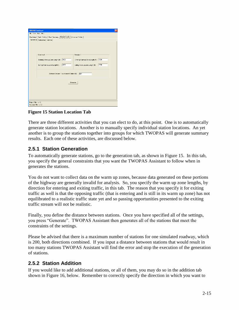
Figure 15 Station Location Tab

There are three different activities that you can elect to do, at this point. One is to automatically

generate station locations. Another is to manually specify individual station locations. An yet

another is to group the stations together into groups for which TWOPAS will generate summary

results. Each one of these activities, are discussed below.

2.5.1 Station Generation

To automatically generate stations, go to the generation tab, as shown in Figure 15. In this tab,

you specify the general constraints that you want the TWOPAS Assistant to follow when in

generates the stations.

You do not want to collect data on the warm up zones, because data generated on these portions

of the highway are generally invalid for analysis. So, you specify the warm up zone lengths, by

direction for entering and exiting traffic, in this tab. The reason that you specify it for exiting

traffic as well is that the opposing traffic (that is entering and is still in its warm up zone) has not

equilibrated to a realistic traffic state yet and so passing opportunities presented to the exiting

traffic stream will not be realistic.

Finally, you define the distance between stations. Once you have specified all of the settings,

you press “Generate”. TWOPAS Assistant then generates all of the stations that meet the

constraints of the settings.

Please be advised that there is a maximum number of stations for one simulated roadway, which

is 200, both directions combined. If you input a distance between stations that would result in

too many stations TWOPAS Assistant will find the error and stop the execution of the generation

of stations.

2.5.2 Station Addition

If you would like to add additional stations, or all of them, you may do so in the addition tab

shown in Figure 16, below. Remember to correctly specify the direction in which you want to

2-16

add the station. To help you keep track of why you added this station, you may enter a

description as well. We will learn about the subsection related settings in the next section.

As usual, you should note the delete button and the navigation buttons “<<” and “>>”. These

allow you to navigate to and remove any stations from the currently defined roadway. Notice

that when you press the navigation buttons the sequence number changes to that of the station to

which you have navigated. When you delete or add a station the sequence numbers will

automatically be changed.

Figure 16 Station Addition Tab

You may add a new station, update an existing one, or delete an existing one. To do this, press

the “add”, “update”, and “delete” buttons, respectively. Again, to save new or modified

information you must press the update button.

2.5.3 Station Subsections

As mentioned earlier, you may group contiguous stations into groups over which you want to

summarize data. For each group of data, a set of summary data will be generated. You may

define several stations for a given direction and you do so by specifying the from-station and the

to-station. You may specify these by manually entering their respective locations or you may

use the pull down menu of all existing stations that you have located on the highway.

2-17

Figure 17 Station Subsections Tab

As always, press “save” after you have entered data into the fields, as shown in Figure 17.

2.6 Create the Input File and Run TWOPAS

After you have entered the run setup, roadway, traffic, and station data, you are ready to export

the TWOPAS input file and run a TWOPAS simulation. Go to the TWOPAS Assistant menu

bar and select “File”, then “Export”, and then “TwoPas Input” (see Figure 18, below). A pop-up

window will then prompt you to specify a file name of the file type *.INP.

Figure 18 Exporting TWOPAS Input File

Warnings will appear if you did not enter any records in some portions of the database tables.

For example, you may not have any crawl regions specified in the database crawl region table. If

this is the case then you will get a warning as shown in Figure 19.

2-18

Figure 19 No-Records Error For TWOPAS Input File Export

To run TWOPAS, go to the TWOPAS Assistant menu bar, select “Run”, and then select

“Twopas” (if you are running in a Windows 2000 environment select TWOPAS98), as shown in

Figure 20.

Figure 20 Running TWOPAS

A pop-up window will appear (see Figure 21), where you need to define the input file path and

name of the input file. Select the ‘…’ button and browse for, and select, the input file you

created. “Run TWOPAS” to run the TWOPAS simulation model, using the input file that you

specified. TWOPAS will run using the input file that you selected and will create output data

files from which you extract performance measures for your analysis.

Figure 21 Selecting a TWOPAS File to Run

3-19

3 Viewing and Reading the Summary Output File To view the output of a TWOPAS simulation run, the most useful file to access is the *.SUM

file. This file contains a variety of information. To view this *.SUM file, press “View” on the

menu bar and select “TWOPAS summary output file” (see Figure 22). Select the file appearing

in the file browser window that has the input data file name with a “.sum” prefix (i.e., [input file

name].sum). There may be a variety of files in the directory that have the *.SUM prefix. So,

make sure to select the one that the file name [name of input file you created].SUM.

Figure 22 Viewing TWOPAS Summary Output File

The “*.sum” file is a summary output file created based on data extracted from a much more

detailed and less useful output file. See the below figure for a sample printout of the “*.sum”

file. The following discussion describes the output data and their respective locations in this file,

where locations are specified in lines and, when applicable, in columns.

3-20

1 ***** PROGRAM TWOPAS: RURAL TRAFFIC SIMULATION; OUTPUT SUMMARY *****

1RUN NO. 1 sensitivity test1

ROAD:TEST1 TRAF:TEST1 OBS:TEST1 DATE: 9/27/01 TIME:11:17 NB SB

RANDOM NUMBERS: 313255 741279 124073 763253 262453

0 WARM TIME= 25.000 MINUTES TEST TIME= 60.000 MINUTES TOTAL TIME= 85.000 MINUTES

OVERALL TRAVEL TIME= 63.5 SEC, S.D.= 2.7 SEC

OVERALL % TIME NOT IN STATE 1: DIR1= 62.4 DIR2= 60.7 COMB= 61.5

LENGTH= 52800.

DIR1 FLOW RATE= 600. ENTERING % FOLL.= 33. DIR2 FLOW RATE= 600. ENTERING % FOLL.= 33.

TRAF COMPOSITION DIR 1 TRUCKS= 4.0 RVS= 0.0 CARS= 96.0 DIR 2 TRUCKS= 4.0 RVS= 0.0 CARS= 96.0

STANDARD DEVIATION DIR 1 TRUCKS= 3.50 RVS= 3.00 CARS= 4.00 DIR 2 TRUCKS= 3.50 RVS= 3.00 CARS= 4.00

SPEEDS DIR 1 TRUCKS= 60.0 RVS= 60.0 CARS= 62.0 DIR 2 TRUCKS= 60.0 RVS= 60.0 CARS= 62.0

*** SUMMARY SPOT CHARACTERISTICS ***

STN LOCATION DIRN NL FLOW %UNIMP %DESSP PSIZE NFOLL SPTRK SPRV SPCAR SPALL %IMP PFOLL #PASS

1 MILEPOST 0.100 1 1 586.0 82.0 84.0 2.9 201.0 59.3 0.0 61.0 60.9 18.0 34.3 0.0

2 MILEPOST 0.200 1 1 587.0 77.0 80.0 2.9 214.0 59.5 0.0 60.6 60.6 23.0 36.5 1.0

3 MILEPOST 0.300 1 1 587.0 75.0 77.0 3.0 230.0 59.7 0.0 60.3 60.3 25.0 39.2 3.0

…

97 MILEPOST 9.700 1 1 585.0 22.0 20.0 7.1 481.0 54.9 0.0 54.9 54.9 78.0 82.2 0.0

98 MILEPOST 9.800 1 1 585.0 20.0 21.0 7.3 483.0 54.8 0.0 54.9 54.9 80.0 82.6 0.0

99 MILEPOST 9.900 1 1 586.0 22.0 21.0 7.2 482.0 55.1 0.0 55.3 55.3 78.0 82.3 0.0

…

301 OPPOSING DIR - MP 9.900 2 1 608.0 82.0 85.0 3.0 222.0 59.5 0.0 61.4 61.3 18.0 36.5 0.0

302 OPPOSING DIR - MP 9.800 2 1 608.0 77.0 81.0 2.9 241.0 59.7 0.0 61.1 61.0 23.0 39.6 1.0

303 OPPOSING DIR - MP 9.700 2 1 608.0 74.0 78.0 2.9 253.0 59.7 0.0 60.9 60.8 26.0 41.6 3.0

…

397 OPPOSING DIR - MP 0.300 2 1 590.0 24.0 23.0 6.9 480.0 55.5 0.0 56.0 56.0 76.0 81.4 0.0

398 OPPOSING DIR - MP 0.200 2 1 590.0 22.0 22.0 6.9 480.0 55.6 0.0 56.0 56.0 78.0 81.4 0.0

399 OPPOSING DIR - MP 0.100 2 1 590.0 24.0 23.0 7.0 481.0 55.8 0.0 56.4 56.3 76.0 81.5 0.0

*** SUMMARY INTERVAL INFORMATION ***

DIRN FROM TO DIST SPEED TTIME MTIME TFDLY PTD %UNIMP PR1 PR2 VTIME VPH PASS1L PASS2L VEH-MILES GEDLY

1 1 99 51744. 56.7 367220. 63.5 5.1 70.2 37.6 0.02 0.00 622.4 590. 136 0 5785.56 0.0

2 1 99 51744. 57.4 370284. 62.5 4.2 69.4 39.3 0.03 0.00 613.0 604. 162 0 5900.89 0.0

1 10 99 46992. 56.4 335306. 63.8 5.4 72.5 34.7 0.02 0.00 567.9 590. 108 0 5257.14 0.0

2 10 99 46992. 57.1 337536. 62.8 4.4 71.5 36.5 0.02 0.00 559.3 604. 127 0 5353.97 0.0

COMPUTER TIME FOR THIS RUN WAS: 7.25 SEC.

4-21

A large amount of data is presented in the *.SUM file, so this description of the file will

focus on those elements that are of primary importance to the operational analysis of two

lane highways. In the HCM 2000 procedures, the measures of effectiveness that are used

are average travel speed and percent time spent following. The *.SUM file contains

measures for both of these in a variety of forms.

In row 5 of the first area of output, is the measure, OVERALL % TIME IN STATE 1.

This is the direct measure of PTSF output by TWOPAS. Notice that there are three

values reported, where two values are for directions one and two and the other is a

combination of the two.

In the second area of output, labeled “Summary Spot Characteristics”, there is a row of

information for each observation point specified in the observation file. First the

information for direction one is presented for each observation point. Then the

information for direction two is presented. Notice that the location of each observation

station is given in terms of ascending mileposts in direction one.

Average travel speed for the traffic stream is reported in the column labeled “SPALL”,

where the average travel speed for trucks, RVs, and cars precede it. The spot measure of

PTSF is given in the column labeled “%IMP” and the spot measure of PF is given in the

column labeled %FOLL

Finally, in the last area of output labeled “Summary Interval Information” is given data

summarized over the facility. The first two rows are for data summarized over all of the

observation stations, where the first row is for direction one and the second is for

direction 2. If an observation interval is set up other than the entire length of the facility

then a third and a fourth row will be output as well, one row for each direction (as is the

case for the file shown in the above figure).

Average travel speed for a given direction is given in the column labeled “SPEED”. The

measure of PF is given in the column labeled PTD and %UNIMP is given in another

column, where PTSF = 100 - %UNIMP.

4 The TWOPAS Output Processor Reading and comparing output in text files can be cumbersome. The purpose of the

TWOPAS Output Processor is to improve access to TWOPAS results. To open the

processor, go to the menu bar and press “Run” then select “Output Processor” (see Figure

23). Output Processor window will open as shown in Figure 24. There are several basic

tasks in the Processor and they are as follows:

1. Open the summary files

2. Organize summary files into useful groups to look at, and compare, statistical

means

3. Read in the summary files

4. View the summary data, summarized over all of the stations

5. View the station data, by group, in graphs

4-22

Figure 23 Starting TWOPAS Output Processor

Figure 24 TWOPAS Output Processor Window

4.1 Open the summary files

You can open up to 3 output files during a Output Processor session, although 12

positions are shown. Open files as shown in Figure 25.

Figure 25 Opening a File for Output Processor

4-23

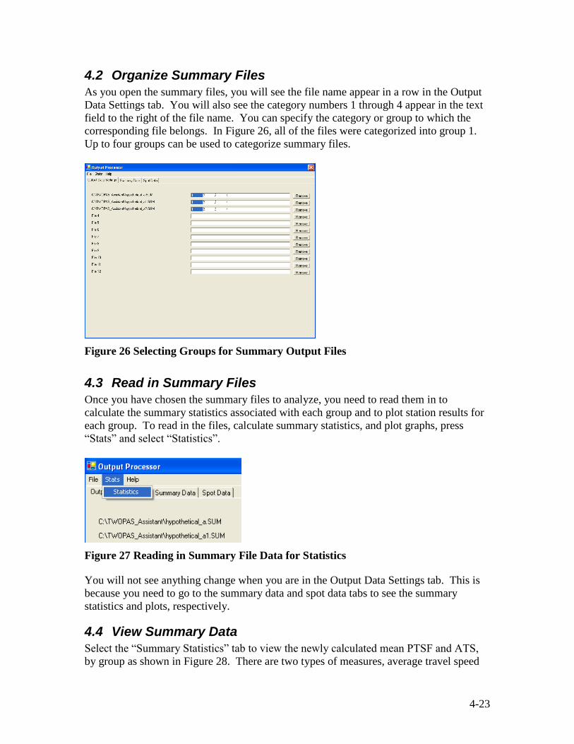
4.2 Organize Summary Files

As you open the summary files, you will see the file name appear in a row in the Output

Data Settings tab. You will also see the category numbers 1 through 4 appear in the text

field to the right of the file name. You can specify the category or group to which the

corresponding file belongs. In Figure 26, all of the files were categorized into group 1.

Up to four groups can be used to categorize summary files.

Figure 26 Selecting Groups for Summary Output Files

4.3 Read in Summary Files

Once you have chosen the summary files to analyze, you need to read them in to

calculate the summary statistics associated with each group and to plot station results for

each group. To read in the files, calculate summary statistics, and plot graphs, press

“Stats” and select “Statistics”.

Figure 27 Reading in Summary File Data for Statistics

You will not see anything change when you are in the Output Data Settings tab. This is

because you need to go to the summary data and spot data tabs to see the summary

statistics and plots, respectively.

4.4 View Summary Data

Select the “Summary Statistics” tab to view the newly calculated mean PTSF and ATS,

by group as shown in Figure 28. There are two types of measures, average travel speed

4-24

(ATS) and percent time spent following (PTSF). PTSF is give by direction as well as for

both direction combined. On the other hand, ATS is only reported for both directions

combined.

Figure 28 Summary Statistics

4.5 View Station Data

To view station data, select the spot data tab, as shown in Figure 29. Again, this is the

average PTSF, as it varies along the simulated highway section. To view the other

graphs, select their corresponding tabs.

Figure 29 Viewing Station (Spot) Data

If you want to compare two or more different groups at one time then you need to read

the summary files into the different groups, when in the Output Data Settings tab (see

Figure 30).

4-25

Figure 30 Specifying Multiple Groups in Output Data Settings Tab

The resulting summary data and graph are shown in Figure 31.

a) Summary Statistics

b) Graph of PTSF for Direction 1

Figure 31 Viewing Data from Multiple Groups