Embed Size (px)
Citation preview

Introduction to the Partitioned Global Address Space (PGAS) Programming Model David E. Hudak, Ph.D. Program Director for HPC Engineering [email protected]

Overview
• Module 1: PGAS Fundamentals
• Module 2: UPC
• Module 3: pMATLAB
• Module 4: Asynchronous PGAS and X10
2

Introduction to PGAS– The Basics
PGAS Model
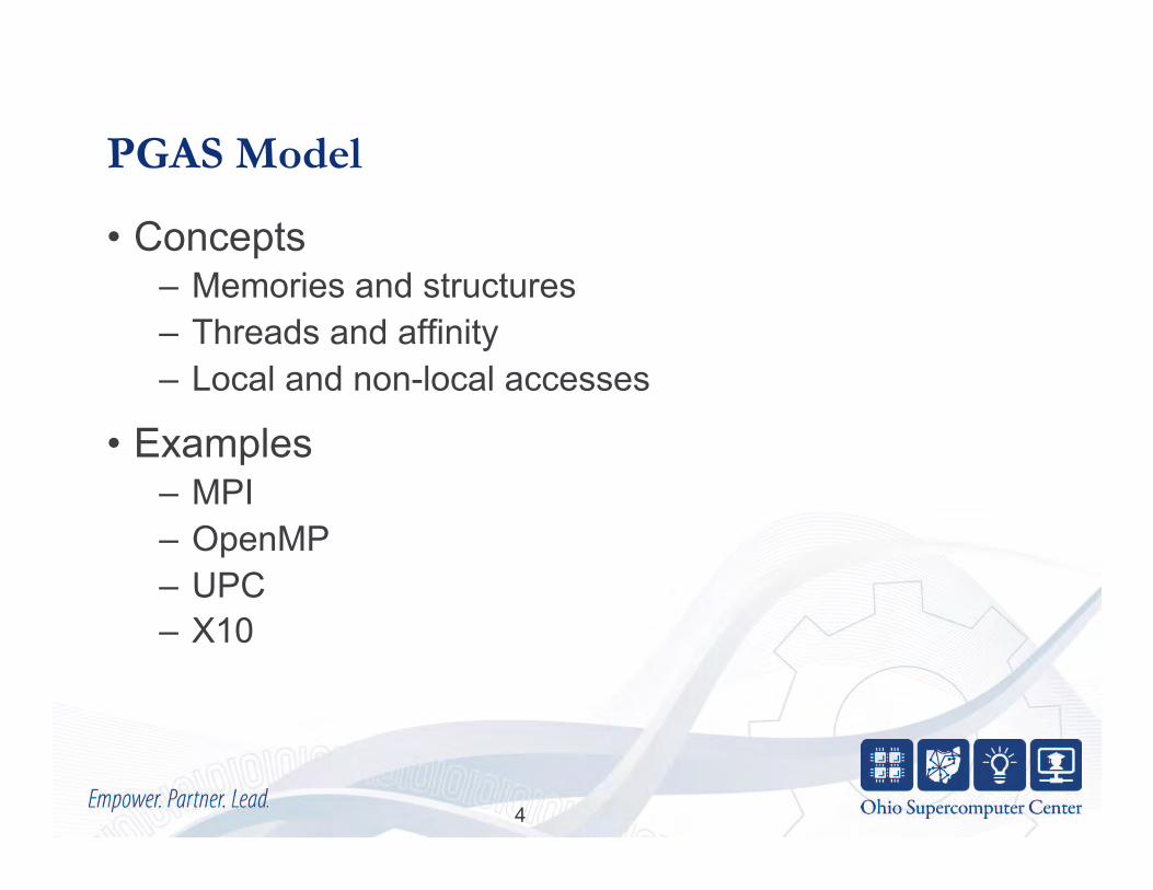
• Concepts – Memories and structures – Threads and affinity – Local and non-local accesses
• Examples – MPI – OpenMP – UPC – X10
4

Software Memory Examples
• Executable Image
• Memories • Static memory
• data segment • Heap memory
• Holds allocated structures • Grows from bottom of
static data region • Stack memory
• Holds function call records • Grows from top of stack
segment
5

Memories and Structures
• Software Memory – Distinct logical storage area in a
computer program (e.g., heap or stack) – For parallel software, we use multiple
memories • Structure
– Collection of data created by program execution (arrays, trees, graphs, etc.)
• Partition – Division of structure into parts
• Mapping – Assignment of structure parts to
memories
6
� � � � � �
� � � � � � � � �� � �
�
�
�
�
� �
� �

Threads
• Units of execution • Structured threading
– Dynamic threads: program creates threads during execution (e.g., OpenMP parallel loop)
– Static threads: same number of threads running for duration of program
• Single program, multiple data (SPMD)
• We will defer unstructured threading
7
� � � � � �

Affinity and Nonlocal Access
• Affinity is the association of a thread to a memory
– If a thread has affinity with a memory, it can access its structures
– Such a memory is called a local memory
• Nonlocal access – Thread 0 wants part B – Part B in Memory 1 – Thread 0 does not have
affinity to memory 1
8
� �
� �
� �
� �
� �
� �
� �
� �

Comparisons
Thread Count
Memory Count
Nonlocal Access
Traditional 1 1 N/A OpenMP Either 1 or p 1 N/A MPI p p No. Message required. C+CUDA 1+p 2 (Host/device) No. DMA required. UPC, CAF, pMatlab
p p Supported.
X10, Asynchronous PGAS
p q Supported.
9

Introduction to PGAS - UPC David E. Hudak, Ph.D.
Slides adapted from some by Tarek El-Ghazawi (GWU) Kathy Yelick (UC Berkeley) Adam Leko (U of Florida)

Outline of talk
1. Background
2. UPC memory/execution model
3. Data and pointers
4. Dynamic memory management
5. Work distribution/synchronization
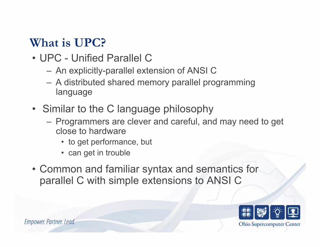
What is UPC? • UPC - Unified Parallel C
– An explicitly-parallel extension of ANSI C – A distributed shared memory parallel programming
language
• Similar to the C language philosophy – Programmers are clever and careful, and may need to get
close to hardware • to get performance, but • can get in trouble
• Common and familiar syntax and semantics for parallel C with simple extensions to ANSI C

Players in the UPC field
• UPC consortium of government, academia, HPC vendors, including:
– ARSC, Compaq, CSC, Cray Inc., Etnus, GWU, HP, IBM, IDA CSC, Intrepid Technologies, LBNL, LLNL, MTU, NSA, UCB, UMCP, UF, US DoD, US DoE, OSU
– See http://upc.gwu.edu for more details
!$
Hardware support
• Many UPC implementations are available – Cray: X1, X1E – HP: AlphaServer SC and Linux Itanium (Superdome)
systems – IBM: BlueGene and AIX – Intrepid GCC: SGI IRIX, Cray T3D/E, Linux Itanium
and x86/x86-64 SMPs – Michigan MuPC: “reference” implementation – Berkeley UPC Compiler: just about everything else

!%
General view
A collection of threads operating in a partitioned global address space that is logically distributed among threads. Each thread has affinity with a portion of the globally shared address space. Each thread has also a private space.
Elements in partitioned global space belonging to a thread are said to have affinity to that thread.

!&
First example: sequential vector addition
//vect_add.c
#define N 1000
int v1[N], v2[N], v1plusv2[N];
void main()
{
int i;
for (i=0; i<N; i++)
v1plusv2[i]=v1[i]+v2[i];
}
!'
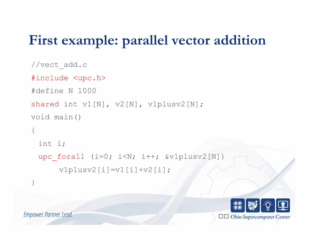
First example: parallel vector addition
//vect_add.c
#include <upc.h>
#define N 1000
shared int v1[N], v2[N], v1plusv2[N];
void main()
{
int i;
upc_forall (i=0; i<N; i++; &v1plusv2[N])
v1plusv2[i]=v1[i]+v2[i];
}

!(
Outline of talk
1. Background
2. UPC memory/execution model
3. Data and pointers
4. Dynamic memory management
5. Work distribution/synchronization

!)
UPC memory model
• A pointer-to-shared can reference all locations in the shared space
• A pointer-to-local (“plain old C pointer”) may only reference addresses in its private space or addresses in its portion of the shared space
• Static and dynamic memory allocations are supported for both shared and private memory

"
UPC execution model
• A number of threads working independently in SPMD fashion
– Similar to MPI – MYTHREAD specifies thread index (0..THREADS-1) – Number of threads specified at compile-time or run-time
• Synchronization only when needed – Barriers – Locks – Memory consistency control

"!
Outline of talk
1. Background
2. UPC memory/execution model
3. Data and pointers
4. Dynamic memory management
5. Work distribution/synchronization
""
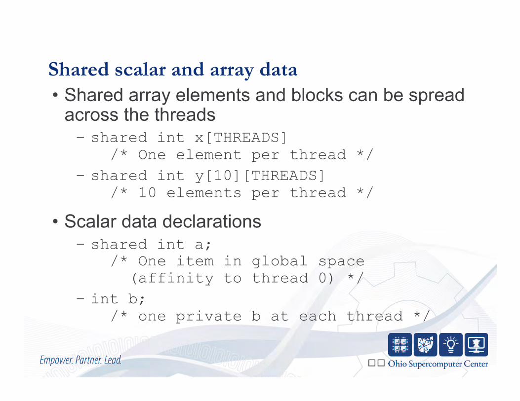
Shared scalar and array data • Shared array elements and blocks can be spread
across the threads – shared int x[THREADS] /* One element per thread */
– shared int y[10][THREADS] /* 10 elements per thread */
• Scalar data declarations – shared int a; /* One item in global space (affinity to thread 0) */
– int b; /* one private b at each thread */
"#
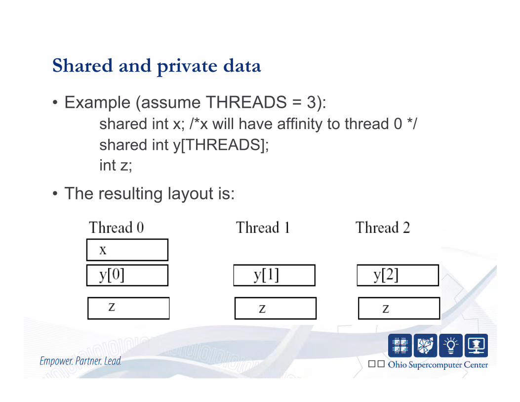
Shared and private data
• Example (assume THREADS = 3): shared int x; /*x will have affinity to thread 0 */ shared int y[THREADS]; int z;
• The resulting layout is:

"$
Shared data
shared int A[2][2*THREADS];
will result in the following data layout:
Remember: C uses row-major ordering

"%
Blocking of shared arrays • Default block size is 1
• Shared arrays can be distributed on a block per thread basis, round robin, with arbitrary block sizes.
• A block size is specified in the declaration as follows:
– shared [block-size] array [N]; – e.g.: shared [4] int a[16];

"&
Blocking of shared arrays
• Block size and THREADS determine affinity
• The term affinity means in which thread’s local shared-memory space, a shared data item will reside
• Element i of a blocked array has affinity to thread:
"'
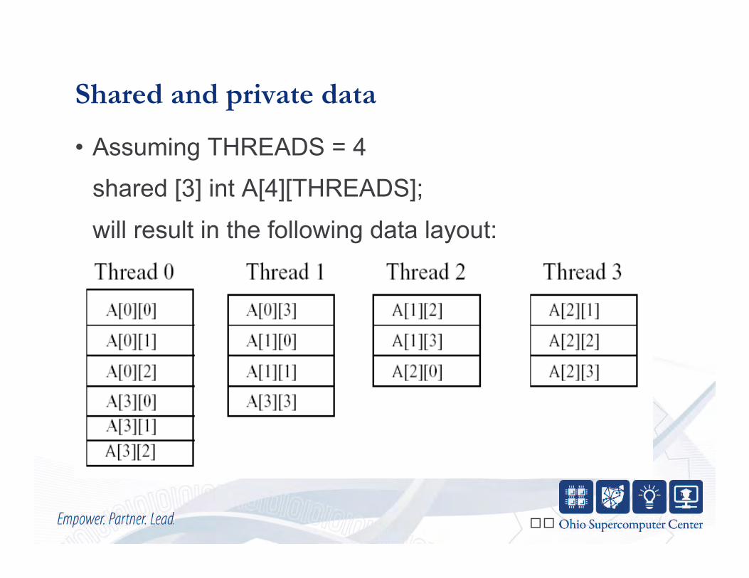
Shared and private data
• Assuming THREADS = 4
shared [3] int A[4][THREADS];
will result in the following data layout:

"(
Shared and private data summary
• Shared objects placed in memory based on affinity
• Affinity can be also defined based on the ability of a thread to refer to an object by a private pointer
• All non-array scalar shared qualified objects have affinity with thread 0
• Threads may access shared and private data

")
UPC pointers
• Pointer declaration: – shared int *p;
• p is a pointer to an integer residing in the shared memory space
• p is called a pointer to shared
• Other pointer declared same as in C – int *ptr; – “pointer-to-local” or “plain old C pointer,” can be used to
access private data and shared data with affinity to MYTHREAD

#
Pointers in UPC

#!
Pointers in UPC • How to declare them?
– int *p1; /* private pointer pointing locally */ – shared int *p2; /* private pointer pointing into the shared space */
– int *shared p3; /* shared pointer pointing locally */
– shared int *shared p4; /* shared pointer pointing into the shared space */

#"
Pointers in UPC
• What are the common usages? – int *p1; /* access to private data or to local shared data */
– shared int *p2; /* independent access of threads to data in shared space */
– int *shared p3; /* not recommended*/ – shared int *shared p4; /* common access of all threads to data in the shared space*/

##
Outline of talk
1. Background
2. UPC memory/execution model
3. Data and pointers
4. Dynamic memory management
5. Work distribution/synchronization

#$
Dynamic memory allocation
• Dynamic memory allocation of shared memory is available in UPC
• Functions can be collective or not
• A collective function has to be called by every thread and will return the same value to all of them

#%
Global memory allocation
shared void *upc_global_alloc(size_t nblocks, size_t nbytes);
nblocks : number of blocks nbytes : block size
• Non collective, expected to be called by one thread • The calling thread allocates a contiguous memory
space in the shared space
• If called by more than one thread, multiple regions are allocated and each thread which makes the call gets a different pointer
• Space allocated per calling thread is equivalent to : shared [nbytes] char[nblocks * nbytes]

#&
Collective global memory allocation shared void *upc_all_alloc(size_t nblocks, size_t nbytes);
nblocks: number of blocks nbytes: block size
• This function has the same result as upc_global_alloc. But this is a collective function, which is expected to be called by all threads
• All the threads will get the same pointer • Equivalent to : shared [nbytes] char[nblocks * nbytes]

#'
Freeing memory
void upc_free(shared void *ptr);
• The upc_free function frees the dynamically allocated shared memory pointed to by ptr
• upc_free is not collective

#(
Some memory functions in UPC * Equivalent of memcpy :
– upc_memcpy(dst, src, size) /* copy from shared to shared */
– upc_memput(dst, src, size) /* copy from private to shared */
– upc_memget(dst, src, size) /* copy from shared to private */
* Equivalent of memset: – upc_memset(dst, char, size) /* initialize shared memory with a character */

#)
Outline of talk
1. Background
2. UPC memory/execution model
3. Data and pointers
4. Dynamic memory management
5. Work distribution/synchronization

$
Work sharing with upc_forall() • Distributes independent iterations • Each thread gets a bunch of iterations • Affinity (expression) field determines how to distribute
work • Simple C-like syntax and semantics
upc_forall (init; test; loop; expression) statement;
• Function of note: upc_threadof(shared void *ptr)
returns the thread number that has affinity to the pointer-to-shared

$!
Synchronization
• No implicit synchronization among the threads
• UPC provides the following synchronization mechanisms:
– Barriers – Locks – Fence – Spinlocks (using memory consistency model)

$"
Synchronization: barriers
• UPC provides the following barrier synchronization constructs:
– Barriers (Blocking) • upc_barrier {expr};
– Split-Phase Barriers (Non-blocking) • upc_notify {expr}; • upc_wait {expr}; • Note: upc_notify is not blocking, upc_wait is

$#
Synchronization: fence
• UPC provides a fence construct – Equivalent to a null strict reference, and has the syntax
• upc_fence; – Null strict reference:
• {static shared strict int x; x=x;}
• Ensures that all shared references issued before the upc_fence are complete

$$
Synchronization: locks
• In UPC, shared data can be protected against multiple writers : – void upc_lock(upc_lock_t *l) – int upc_lock_attempt(upc_lock_t *l) //returns 1 on success and 0 on failure
– void upc_unlock(upc_lock_t *l)
• Locks can be allocated dynamically. Dynamically allocated locks can be freed
• Dynamic locks are properly initialized and static locks need initialization

Introduction to PGAS - pMatlab
Credit: Slides based on some from Jeremey Kepner http://www.ll.mit.edu/mission/isr/pmatlab/pmatlab.html

Agenda
• Overview
• pMatlab Execution (SPMD) – Replicated arrays
• Distributed arrays – Maps – Local components
46

Not real PGAS
• PGAS – Partitioned Global Address Space • MATLAB doesn’t expose address space
– Uses implicit memory management – User creates arrays – MATLAB interpreter allocates/frees the memory
• So, when I say PGAS in MATLAB, I mean – Running multiple copies of the interpreter – Distributed arrays: allocating a single (logical) array as a collection
of local (physical) array components
• Multiple implementations – Open source: MIT Lincoln Labs’ pMatlab + OSC bcMPI – Commercial: Mathworks’ Parallel Computing Toolbox, Interactive
Supercomputing (now Microsoft) Star-P
47
http://www.osc.edu/bluecollarcomputing/applications/bcMPI/index.shtml

Serial Program
• Matlab is a high level language • Allows mathematical expressions to be written concisely • Multi-dimensional arrays are fundamental to Matlab
Y(:,:) = X + 1;!
X = zeros(N,N);!Y = zeros(N,N);!
Matlab

Pid=Np-1!
Pid=1!Pid=0!
Parallel Execution
• Run NP (or Np) copies of same program – Single Program Multiple Data (SPMD)
• Each copy has a unique PID (or Pid) • Every array is replicated on each copy of the program
Y(:,:) = X + 1;!
X = zeros(N,N);!Y = zeros(N,N);!
pMatlab

Pid=Np-1!
Pid=1!Pid=0!
Distributed Array Program
• Use map to make a distributed array • Tells program which dimension to distribute data • Each program implicitly operates on only its own data
(owner computes rule)
Y(:,:) = X + 1;!
XYmap = map([Np 1],{},0:Np-1);!X = zeros(N,N,XYmap);!Y = zeros(N,N,XYmap);!
pMatlab

Explicitly Local Program
• Use local function to explicitly retrieve local part of a distributed array
• Operation is the same as serial program, but with different data in each process (recommended approach)
Yloc(:,:) = Xloc + 1;!
XYmap = map([Np 1],{},0:Np-1);!Xloc = local(zeros(N,N,XYmap));!Yloc = local(zeros(N,N,XYmap));!
pMatlab

Parallel Data Maps
• A map is a mapping of array indices to processes • Can be block, cyclic, block-cyclic, or block w/overlap • Use map to set which dimension to split among processes
Xmap=map([Np 1],{},0:Np-1)!
Matlab
0 1 2 3 Computer
PID! Pid!
Array
Xmap=map([1 Np],{},0:Np-1)!
Xmap=map([Np/2 2],{},0:Np-1)!

Maps and Distributed Arrays
Amap = map([Np 1],{},0:Np-1);
Process Grid
A = zeros(4,6,Amap);
0 0 0 0
0 0 0 0
0 0 0 0
0 0 0 0
0 0 0 0
0 0 0 0
P0 P1 P2 P3
List of processes
pMatlab constructors are overloaded to take a map as an argument, and return a distributed array.
A =
Distribution {}=default=block

Parallelizing Loops
• The set of loop index values is known as an iteration space
• In parallel programming, a set of processes cooperate in order to complete a single task
• To parallelize a loop, we must split its iteration space among processes
54

loopSplit Construct
• parfor is a neat construct that is supported by Mathworks’ PCT
• ParaM’s equivalent is called loopSplit
• Why loopSplit and not parfor? That is a subtle question…
55

Global View vs. Local View
• In parallel programming, a set of processes cooperate in order to complete a single task
• The global view of the program refers to actions and data from the task perspective
– OpenMP programming is an example of global view
• parfor is a global view construct
56

Gobal View vs. Local View (con’t)
• The local view of the program refers to actions and data within an individual process
• Single Program-Multiple Data (SPMD) programs provide a local view
– Each process is an independent execution of the same program
– MPI programming is an example of SPMD
• ParaM uses SPMD • loopSplit is the SPMD
equivalent of parfor
57

loopSplit Example
• Monte Carlo approximation of
• Algorithm – Consider a circle of radius 1 – Let N = some large number (say 10000) and count = 0 – Repeat the following procedure N times
• Generate two random numbers x and y between 0 and 1 (use the rand function)
• Check whether (x,y) lie inside the circle • Increment count if they do
– Pi_value = 4 * count / N
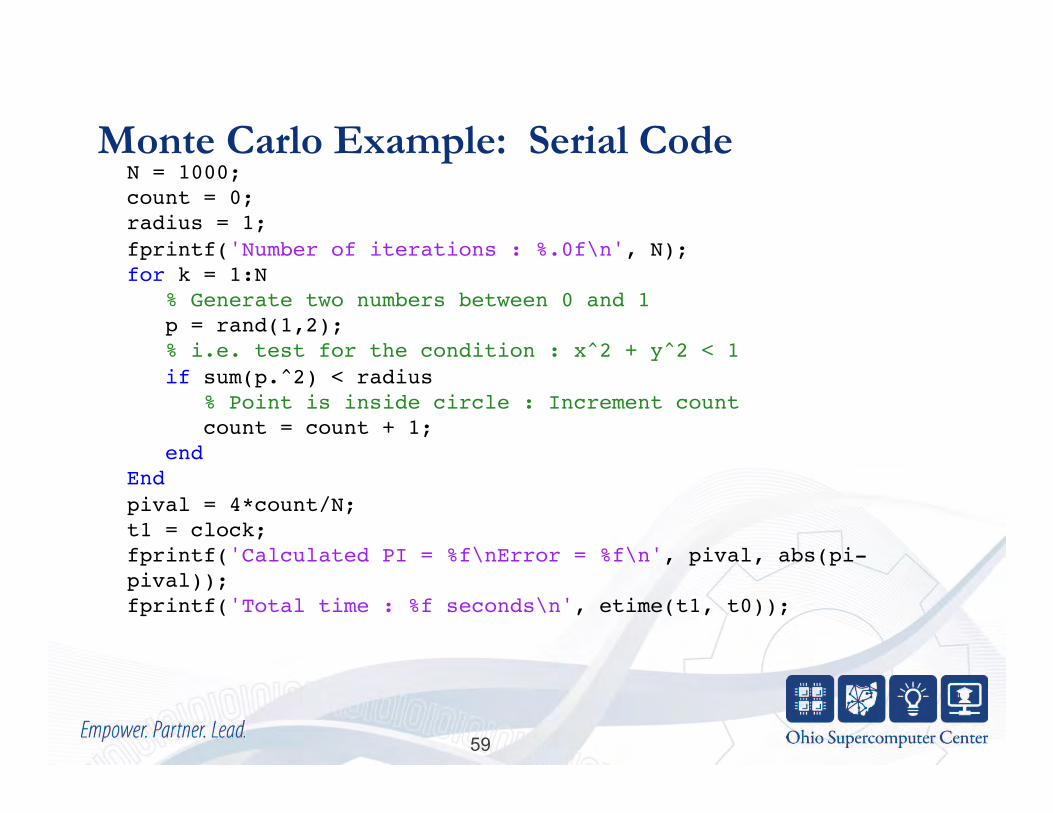
Monte Carlo Example: Serial Code
59
N = 1000;!count = 0;!radius = 1;!fprintf('Number of iterations : %.0f\n', N);!for k = 1:N! % Generate two numbers between 0 and 1! p = rand(1,2);! % i.e. test for the condition : x^2 + y^2 < 1! if sum(p.^2) < radius! % Point is inside circle : Increment count! count = count + 1;! end!End!pival = 4*count/N;!t1 = clock;!fprintf('Calculated PI = %f\nError = %f\n', pival, abs(pi-pival));!fprintf('Total time : %f seconds\n', etime(t1, t0));!
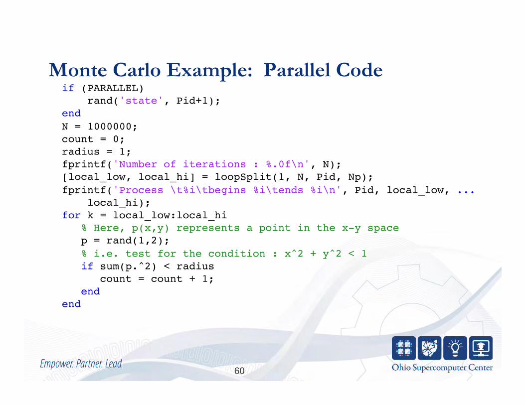
Monte Carlo Example: Parallel Code
60
if (PARALLEL)! rand('state', Pid+1);!end !N = 1000000;!count = 0;!radius = 1;!fprintf('Number of iterations : %.0f\n', N);![local_low, local_hi] = loopSplit(1, N, Pid, Np);!fprintf('Process \t%i\tbegins %i\tends %i\n', Pid, local_low, ...! local_hi); !for k = local_low:local_hi! % Here, p(x,y) represents a point in the x-y space ! p = rand(1,2);! % i.e. test for the condition : x^2 + y^2 < 1! if sum(p.^2) < radius! count = count + 1;! end!end!

Monte Carlo Example: Parallel Output
61
Number of iterations : 1000000!Process 0 begins 1 ends 250000!Process 1 begins 250001 ends 500000!Process 2 begins 500001 ends 750000!Process 3 begins 750001 ends 1000000!Calculated PI = 3.139616!Error = 0.001977!

Monte Carlo Example: Total Count
62
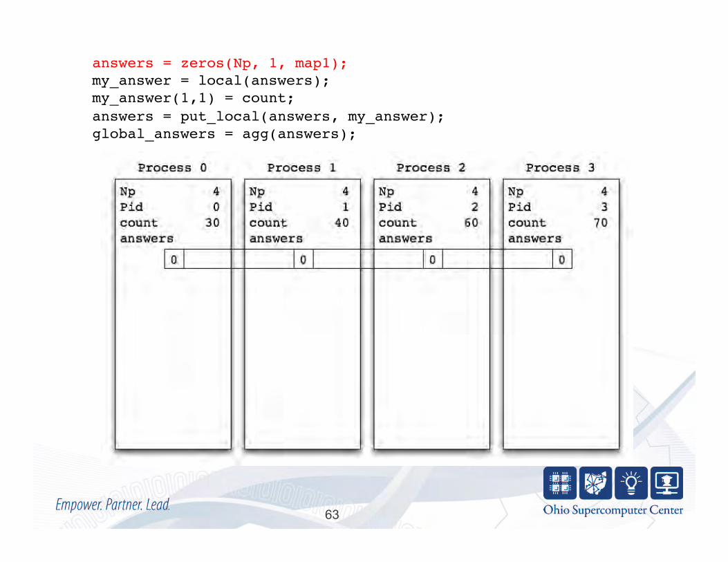
if (PARALLEL)! map1 = map([Np 1], {}, 0:Np-1);!else! map1 = 1;!end!answers = zeros(Np, 1, map1);!my_answer = local(answers);!my_answer(1,1) = count;!answers = put_local(answers, my_answer);!global_answers = agg(answers);!if (Pid == 0) ! global_count = 0;! for i = 1:Np! global_count = global_count + global_answers(i,1);! end! pival = 4*global_count/N;! fprintf(‘PI = %f\nError = %f\n', pival, abs(pi-pival));!end!
63
answers = zeros(Np, 1, map1);!my_answer = local(answers);!my_answer(1,1) = count;!answers = put_local(answers, my_answer);!global_answers = agg(answers);!

64
answers = zeros(Np, 1, map1);!my_answer = local(answers);!my_answer(1,1) = count;!answers = put_local(answers, my_answer);!global_answers = agg(answers);!

65
answers = zeros(Np, 1, map1);!my_answer = local(answers);!my_answer(1,1) = count;!answers = put_local(answers, my_answer);!global_answers = agg(answers);!

66
answers = zeros(Np, 1, map1);!my_answer = local(answers);!my_answer(1,1) = count;!answers = put_local(answers, my_answer);!global_answers = agg(answers);!
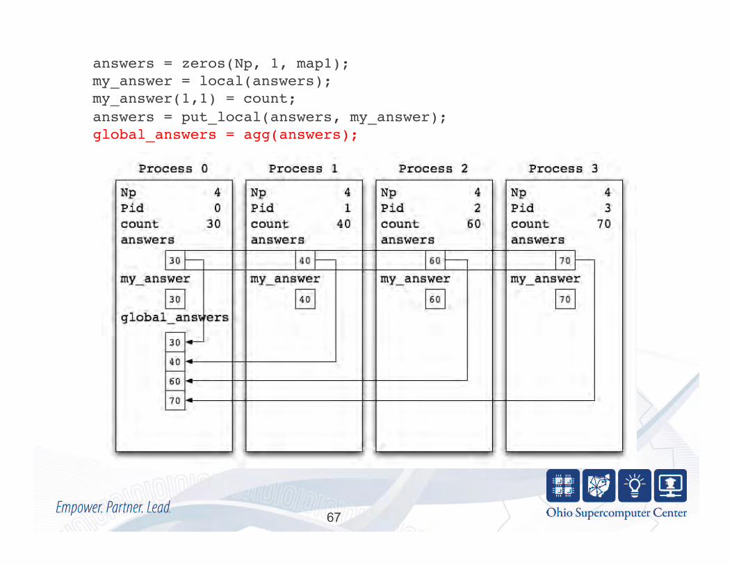
67
answers = zeros(Np, 1, map1);!my_answer = local(answers);!my_answer(1,1) = count;!answers = put_local(answers, my_answer);!global_answers = agg(answers);!

68
if (Pid == 0) ! global_count = 0;! for i = 1:Np! global_count = global_count + global_answers(i,1);!

Introduction to PGAS - APGAS and the X10 Language
Credit: Slides based on some from David Grove, et.al. http://x10.codehaus.org/Tutorials

Outline
• MASC architectures and APGAS
• X10 fundamentals
• Data distributions (points and regions)
• Concurrency constructs
• Synchronization constructs
• Examples
70

Multicore/Accelerator multiSpace Computing (MASC)
• Cluster of nodes
• Each node – Multicore processing
• 2 to 4 sockets/board now • 2, 4, 8 cores/socket now
– Manycore accelerator • Discrete device (GPU) • Integrated w/CPU (Intel “Knights Corner”)
• Multiple memory spaces – Per node memory (accessible by local
cores) – Per accelerator memory
71
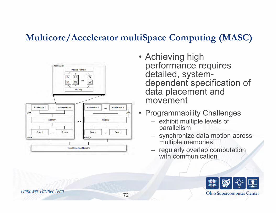
Multicore/Accelerator multiSpace Computing (MASC)
• Achieving high performance requires detailed, system-dependent specification of data placement and movement
• Programmability Challenges – exhibit multiple levels of
parallelism – synchronize data motion across
multiple memories – regularly overlap computation
with communication
72

Every Parallel Architecture has a dominant programming model
Parallel Architecture
Programming Model
Vector Machine (Cray 1)
Loop vectorization(IVDEP)
SIMD Machine (CM-2)
Data parallel (C*)
SMP Machine (SGI Origin)
Threads (OpenMP)
Clusters (IBM 1350)
Message Passing (MPI)
GPGPU (nVidia Tesla)
Data parallel (CUDA)
MASC Asynchronous PGAS?
• MASC Options – Pick a single model
(MPI, OpenMP) – Hybrid code
• MPI at node level • OpenMP at core level • CUDA at accelerator
– Find a higher-level abstraction, map it to hardware
73

X10 Concepts
• Asynchronous PGAS – PGAS model in which threads can be dynamically
created under programmer control – p distinct memories, q distinct threads (p <> q)
• PGAS memories are called places in X10
• PGAS threads are called activities in X10
74

What is X10?
• X10 is a new language developed in the IBM PERCS project as part of the DARPA program on High Productivity Computing Systems (HPCS)
• X10 is an instance of the APGAS framework in the Java family
• X10 – Is more productive than current models – Can support high levels of abstraction – Can exploit multiple levels of parallelism and non-uniform
data access – Is suitable for multiple architectures, and multiple workloads.

X10 Constructs
Fine grained concurrency • async S
Atomicity • atomic S • when (c) S
Global data-structures • points, regions, distributions, arrays
Place-shifting operations • at (P) S
Ordering • finish S • clock
Two basic ideas: Places and Activites

X10 Project Status
• X10 is an open source project (Eclipse Public License) – Documentation, releases, mailing lists, code, etc. all publicly
available via http://x10-lang.org • XRX: X10 Runtime in X10 (14kloc and growing) • X10 1.7.x releases throughout 2009 (Java & C++) • X10 2.0 released November 6, 2009
– Java: Single process (all places in 1 JVM) • any platform with Java 5
– C++: Multi-process (1 place per process) • aix, linux, cygwin, solaris • x86, x86_64, PowerPC, Sparc • x10rt: APGAS runtime (binary only) or MPI (open source)

Overview of Features • Many sequential features of Java
inherited unchanged – Classes (w/ single inheritance) – Interfaces, (w/ multiple
inheritance) – Instance and static fields – Constructors, (static) initializers – Overloaded, over-rideable
methods – Garbage collection
• Structs • Closures • Points, Regions, Distributions,
Arrays
• Substantial extensions to the type system
– Dependent types – Generic types – Function types – Type definitions, inference
• Concurrency – Fine-grained concurrency:
• async (p,l) S – Atomicity
• atomic (s) – Ordering
• L: finish S – Data-dependent
synchronization • when (c) S

Points and Regions • A point is an element of an n-
dimensional Cartesian space (n>=1) with integer-valued coordinates e.g., [5], [1, 2], …
• A point variable can hold values of different ranks e.g.,
– var p: Point = [1]; p = [2,3]; … • Operations
– p1.rank • returns rank of point p1
– p1(i) • returns element (i mod p1.rank) if
i < 0 or i >= p1.rank – p1 < p2, p1 <= p2, p1 > p2, p1 >=
p2 • returns true iff p1 is
lexicographically <, <=, >, or >= p2 • only defined when p1.rank and
p2.rank are equal
• Regions are collections of points of the same dimension
• Rectangular regions have a simple representation, e.g. [1..10, 3..40]
• Rich algebra over regions is provided

Distributions and Arrays
• Distributions specify mapping of points in a region to places
– E.g. Dist.makeBlock(R) – E.g. Dist.makeUnique()
• Arrays are defined over a distribution and a base type
– A:Array[T] – A:Array[T](d)
• Arrays are created through initializers
– Array.make[T](d, init)
• Arrays are mutable (considering immutable arrays)
• Array operations • A.rank ::= # dimensions in
array • A.region ::= index region
(domain) of array • A.dist ::= distribution of array
A • A(p) ::= element at point p,
where p belongs to A.region• A(R) ::= restriction of array
onto region R – Useful for extracting
subarrays

async
• async S – Creates a new child
activity that executes statement S
– Returns immediately – S may reference final
variables in enclosing blocks
– Activities cannot be named
– Activity cannot be aborted or cancelled
Stmt ::= async(p,l) Stmt
cf Cilk’s spawn
// Compute the Fibonacci // sequence in parallel. def run() { if (r < 2) return; val f1 = new Fib(r-1), f2 = new Fib(r-2); finish { async f1.run(); f2.run(); } r = f1.r + f2.r; }

// Compute the Fibonacci // sequence in parallel. def run() { if (r < 2) return; val f1 = new Fib(r-1), f2 = new Fib(r-2); finish { async f1.run(); f2.run(); } r = f1.r + f2.r; }
finish
• L: finish S – Execute S, but wait until all
(transitively) spawned asyncs have terminated.
• Rooted exception model – Trap all exceptions thrown by
spawned activities. – Throw an (aggregate)
exception if any spawned async terminates abruptly.
– Implicit finish at main activity
• finish is useful for expressing “synchronous” operations on (local or) remote data.
Stmt ::= finish Stmt
cf Cilk’s sync

at
• at(p) S – Execute statement S at
place p – Current activity is blocked
until S completes
Stmt ::= at(p) Stmt
// Copy field f from a to b def copyRemoteFields(a, b) { at (b.loc) b.f = at (a.loc) a.f; }
// Increment field f of obj def incField(obj, inc) { at (obj.loc) obj.f += inc; }
// Invoke method m on obj def invoke(obj, arg) { at (obj.loc) obj.m(arg); }

// push data onto concurrent // list-stack val node = new Node(data); atomic { node.next = head; head = node; }
atomic
• atomic S – Execute statement S
atomically – Atomic blocks are
conceptually executed in a single step while other activities are suspended: isolation and atomicity.
• An atomic block body (S) ...
– must be nonblocking – must not create concurrent
activities (sequential) – must not access remote
data (local)
// target defined in lexically // enclosing scope. atomic def CAS(old:Object, n:Object) { if (target.equals(old)) { target = n; return true; } return false; }
Stmt ::= atomic Statement MethodModifier ::= atomic

when
• when (E) S – Activity suspends until a state in
which the guard E is true. – In that state, S is executed
atomically and in isolation. – Guard E is a boolean expression
• must be nonblocking • must not create concurrent
activities (sequential) • must not access remote data
(local) • must not have side-effects (const)
• await (E) – syntactic shortcut for when (E) ;
Stmt ::= WhenStmt WhenStmt ::= when ( Expr ) Stmt | WhenStmt or (Expr) Stmt
class OneBuffer { var datum:Object = null; var filled:Boolean = false; def send(v:Object) { when ( !filled ) { datum = v; filled = true; } } def receive():Object { when ( filled ) { val v = datum; datum = null; filled = false; return v; } } }

Clocks: Motivation • Activity coordination using finish is accomplished by checking for
activity termination • But in many cases activities have a producer-consumer relationship
and a “barrier”-like coordination is needed without waiting for activity termination
– The activities involved may be in the same place or in different places • Design clocks to offer determinate and deadlock-free coordination
between a dynamically varying number of activities.
Activity 0 Activity 1 Activity 2 . . .
Phase 0
Phase 1
. . .

Clocks: Main operations
• var c = Clock.make(); – Allocate a clock, register
current activity with it. Phase 0 of c starts.
• async(…) clocked (c1,c2,…) S • ateach(…) clocked (c1,c2,…) S
• foreach(…) clocked (c1,c2,…) S
• Create async activities registered on clocks c1, c2, …
• c.resume(); – Nonblocking operation that
signals completion of work by current activity for this phase of clock c
• next; – Barrier — suspend until all
clocks that the current activity is registered with can advance. c.resume() is first performed for each such clock, if needed.
• next can be viewed like a “finish” of all computations under way in the current phase of the clock
Fundamental X10 Property
• Programs written using async, finish, at, atomic, clock cannot deadlock
• Intuition: cannot be a cycle in waits-for graph

y
x
(1)
(2)
Because of the time steps, Typically, two grids are used
2D Heat Conduction Problem
• Based on the 2D Partial Differential Equation (1), 2D Heat Conduction problem is similar to a 4-point stencil operation, as seen in (2):

A:!
1.0
n
n
Σ ÷ 4
repeat until max change < ε
Heat Transfer in Pictures
Heat transfer in X10
• X10 permits smooth variation between multiple concurrency styles
– “High-level” ZPL-style (operations on global arrays) • Chapel “global view” style • Expressible, but relies on “compiler magic” for performance
– OpenMP style • Chunking within a single place
– MPI-style • SPMD computation with explicit all-to-all reduction • Uses clocks
– “OpenMP within MPI” style • For hierarchical parallelism • Fairly easy to derive from ZPL-style program.
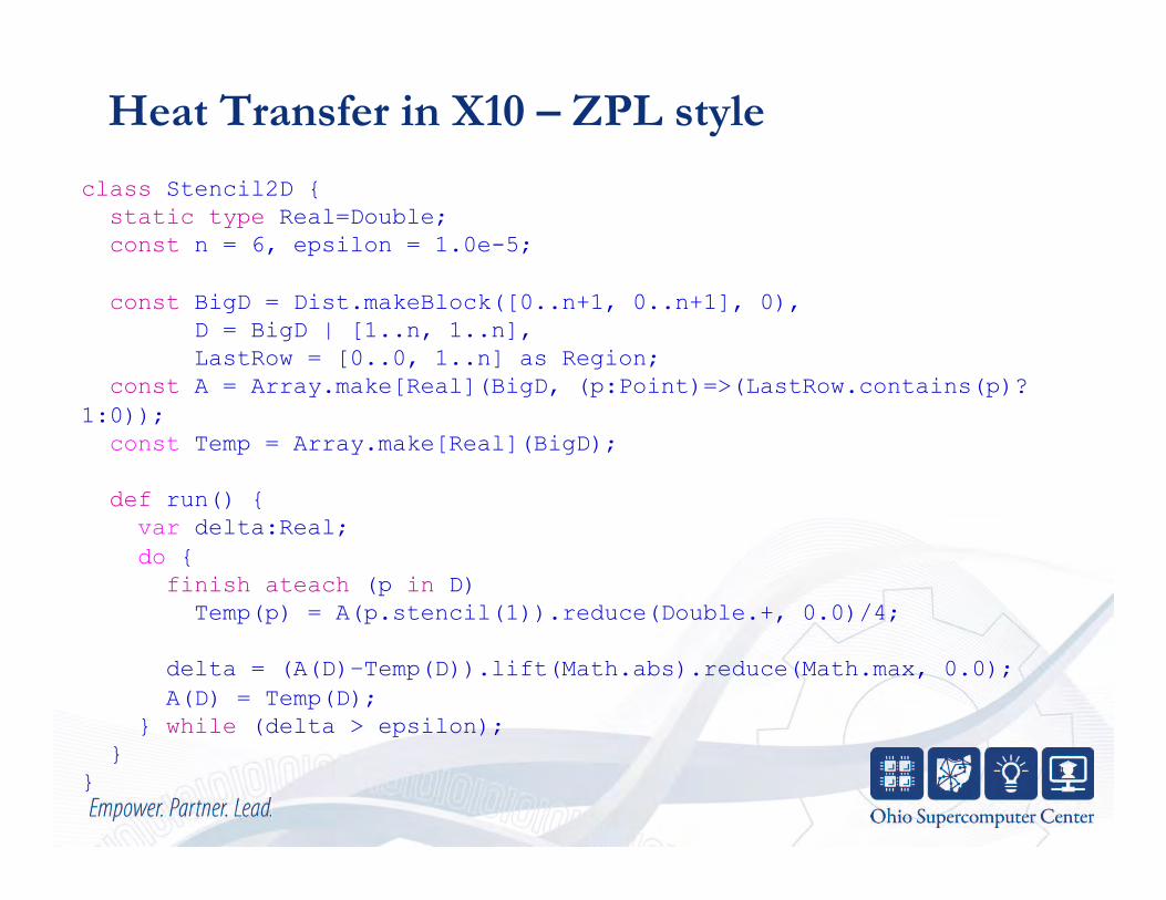
Heat Transfer in X10 – ZPL style
class Stencil2D { static type Real=Double; const n = 6, epsilon = 1.0e-5;
const BigD = Dist.makeBlock([0..n+1, 0..n+1], 0), D = BigD | [1..n, 1..n], LastRow = [0..0, 1..n] as Region; const A = Array.make[Real](BigD, (p:Point)=>(LastRow.contains(p)?1:0)); const Temp = Array.make[Real](BigD);
def run() { var delta:Real; do { finish ateach (p in D) Temp(p) = A(p.stencil(1)).reduce(Double.+, 0.0)/4;
delta = (A(D)–Temp(D)).lift(Math.abs).reduce(Math.max, 0.0); A(D) = Temp(D); } while (delta > epsilon); } }
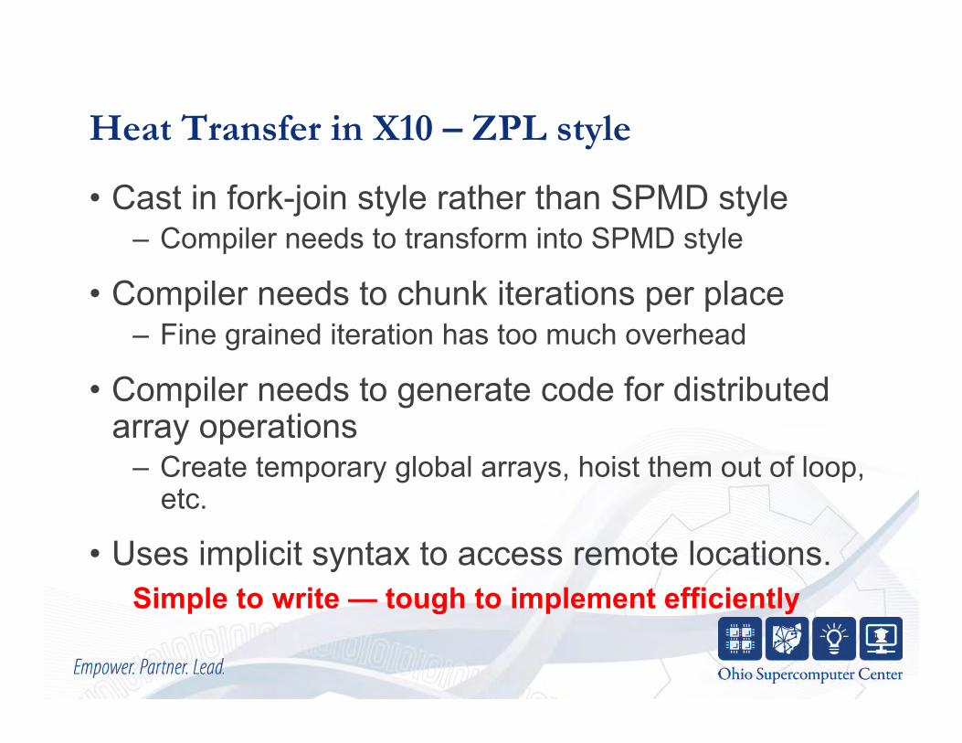
Heat Transfer in X10 – ZPL style
• Cast in fork-join style rather than SPMD style – Compiler needs to transform into SPMD style
• Compiler needs to chunk iterations per place – Fine grained iteration has too much overhead
• Compiler needs to generate code for distributed array operations
– Create temporary global arrays, hoist them out of loop, etc.
• Uses implicit syntax to access remote locations. Simple to write — tough to implement efficiently
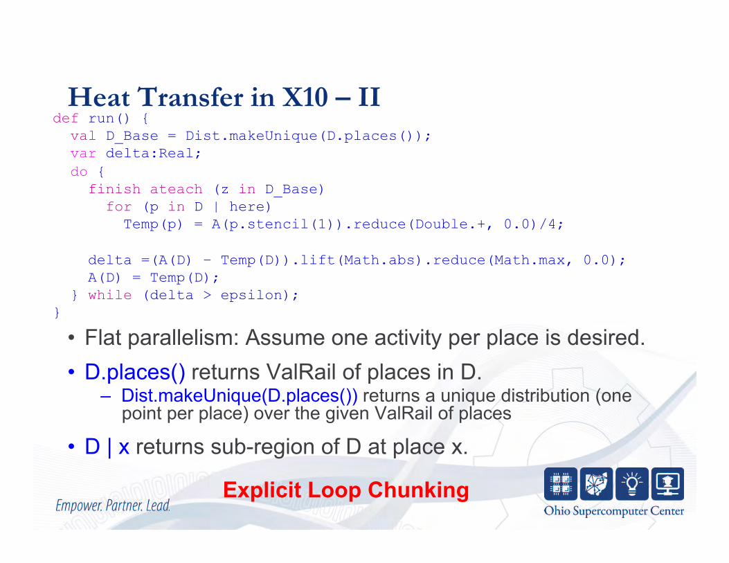
def run() { val D_Base = Dist.makeUnique(D.places()); var delta:Real; do { finish ateach (z in D_Base) for (p in D | here) Temp(p) = A(p.stencil(1)).reduce(Double.+, 0.0)/4;
delta =(A(D) – Temp(D)).lift(Math.abs).reduce(Math.max, 0.0); A(D) = Temp(D); } while (delta > epsilon); }
Heat Transfer in X10 – II
• Flat parallelism: Assume one activity per place is desired. • D.places() returns ValRail of places in D.
– Dist.makeUnique(D.places()) returns a unique distribution (one point per place) over the given ValRail of places
• D | x returns sub-region of D at place x.
Explicit Loop Chunking

Heat Transfer in X10 – III
• Hierarchical parallelism: P activities at place x. – Easy to change above code so P can vary with x.
• DistUtil.block(D,P)(x,q) is the region allocated to the q’th activity in place x. (Block-block division.)
Explicit Loop Chunking with Hierarchical Parallelism
def run() { val D_Base = Dist.makeUnique(D.places()); val blocks = DistUtil.block(D, P); var delta:Real; do { finish ateach (z in D_Base) foreach (q in 1..P) for (p in blocks(here,q)) Temp(p) = A(p.stencil(1)).reduce(Double.+, 0.0)/4;
delta =(A(D)–Temp(D)).lift(Math.abs).reduce(Math.max, 0.0); A(D) = Temp(D); } while (delta > epsilon); }

def run() { finish async { val c = clock.make(); val D_Base = Dist.makeUnique(D.places()); val diff = Array.make[Real](D_Base), scratch = Array.make[Real](D_Base); ateach (z in D_Base) clocked(c) do { diff(z) = 0.0; for (p in D | here) { Temp(p) = A(p.stencil(1)).reduce(Double.+, 0.0)/4; diff(z) = Math.max(diff(z), Math.abs(A(p) - Temp(p))); } next; A(D | here) = Temp(D | here); reduceMax(z, diff, scratch); } while (diff(z) > epsilon); } }
Heat Transfer in X10 – IV
• reduceMax() performs an all-to-all max reduction. SPMD with all-to-all reduction == MPI style
One activity per place == MPI task
Akin to UPC barrier

Heat Transfer in X10 – V
“OpenMP within MPI style”
def run() { finish async { val c = clock.make(); val D_Base = Dist.makeUnique(D.places()); val diff = Array.make[Real](D_Base), scratch = Array.make[Real](D_Base); ateach (z in D_Base) clocked(c) foreach (q in 1..P) clocked(c) var myDiff:Real = 0; do { if (q==1) { diff(z) = 0.0}; myDiff = 0; for (p in blocks(here,q)) { Temp(p) = A(p.stencil(1)).reduce(Double.+, 0.0)/4; myDiff = Math.max(myDiff, Math.abs(A(p) – Temp(p))); } atomic diff(z) = Math.max(myDiff, diff(z)); next; A(blocks(here,q)) = Temp(blocks(here,q)); if (q==1) reduceMax(z, diff, scratch); next; myDiff = diff(z); next; } while (myDiff > epsilon); } }
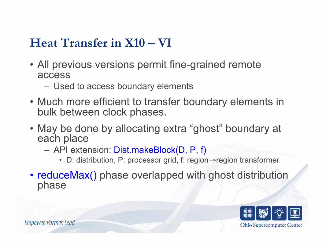
Heat Transfer in X10 – VI
• All previous versions permit fine-grained remote access
– Used to access boundary elements
• Much more efficient to transfer boundary elements in bulk between clock phases.
• May be done by allocating extra “ghost” boundary at each place
– API extension: Dist.makeBlock(D, P, f) • D: distribution, P: processor grid, f: region→region transformer
• reduceMax() phase overlapped with ghost distribution phase


![12th UPC++ - OpenFabricsusing UPC++ [3], a partitioned global address space (PGAS) extension to the C++ language. A. A motivating example The above class of distributed assembly problem](https://img.pdfslide.us/doc/110x75/5e24221ead7b0357425a2a03/12th-upc-openfabrics-using-upc-3-a-partitioned-global-address-space-pgas.jpg)