Introduction to the modelling/tomography tools within ... like described under step 6. 9. Return to the main modelling menu by simply ... Therefore the program searches automatically

Sandmeier geophysical software - REFLEXW guide

Introduction to the modelling/tomography tools within REFLEXW

In the following the different modelling/tomography tools within the modelling menu of REFLEXWare described. The main tools are:2D and 3D Finite difference modelling for seismic and electromagnetic wave propagation (chap. II)2D ray tracing (chap. III)2D- and 3D- transmission and refraction tomography (chap. IV)Chap. I includes the generation of a model. This chapter is a more general one because all tools need amodel to be generated first.Please use in addition to this user’s guide the handbook instructions and the online help.

I. model generation

First the generation of a complete new model isdescribed.

1. Enter the module modelling

2. Choose the wavetype (e.g. electromagneticfor a GPR-modelling or acoustic for araytracing).

3. Enter the min./max. borders of the model(parameters xmin, xmax, zmin, zmax). To beconsidered: z is going from top to bottom withpositive numbers (e.g. zmin=0 and zmax=20).

4. activate the option new. The layer nr. ischanged to 1.

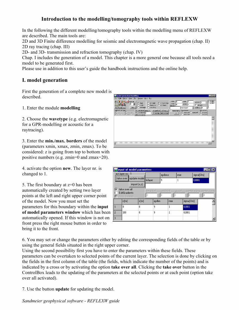
5. The first boundary at z=0 has beenautomatically created by setting two layerpoints at the left and right upper corner pointof the model. Now you must set theparameters for this boundary within the inputof model parameters window which has beenautomatically opened. If this window is not onfront press the right mouse button in order tobring it to the front.

6. You may set or change the parameters either by editing the corresponding fields of the table or byusing the general fields situated in the right upper corner.Using the second possibility first you have to enter the parameters within these fields. Theseparameters can be overtaken to selected points of the current layer. The selection is done by clicking onthe fields in the first column of the table (the fields, which indicate the number of the points) and isindicated by a cross or by activating the option take over all. Clicking the take over button in theControlBox leads to the updating of the parameters at the selected points or at each point (option takeover all activated).

7. Use the button update for updating the model.


8. You may include some new layer points by simply clicking within the main modelling menu. Theactual general model parameters of the fields within the right upper corner of the input of modellingparameter menu are automatically taken over for these new layer points. You may change theseparameters like described under step 6.

9. Return to the main modelling menu by simply activating it or by closing the input of modelparameters menu.

10. activate the option new for the next layer. The layer nr. is changed to 2. 11. For that layer you have to define all layer points and the corresponding model parameters - see step6 to step 9.

12. Additional layers are defined as described for layer 2.

13. All layers must be closed - this means they must start or end at the model border or at any otherlayer boundary. It is not necessary to do this manually but the options extrapolate and hor.extrapol.may be used for that purpose. The interfaces don't have to be entered exactly at the edge, intersectionwith another interface, respectively, but in the vicinity because the option extrapolate makes theautomatic interpolation between two interfaces as well as the extrapolation of the interface to theboundary possible. Therefore the program searches automatically the nearest border at the exposed endand extrapolates in that direction (in the case of an edge, extrapolation in x-, z-direction, respectively,in the case of an interface to the nearest layer point).

PLEASE NOTE: The layer points are sorted automatically from lower x-distance to higher x-distance,i.e. the interface function is unequivocal. Should for example a convolution be given it has to occur bygiving several interfaces, like it is done by the predefined symbols circle and rectangle.

14. Enter a filename and save the model using the speedoption or the option file/save model. 15. For additional features like using predefined symbols, combining existing layers or adding atopography please refer to the handbook instructions under the individual chapters or to the onlinehelp.


II. Finite Difference (FD) modelling

The Finite Difference (FD) modelling tool allows the simulation of electromagnetic or seismic wavepropagation, respectively by means of FD-method for different sources (plane wave, point source aswell as "Exploding-Reflector"-source). As a result a single line or the complete wavefield are storedand can be displayed after.

In the following we are describing the GPR-simulation for a 2D zero-offset section (standard GPR-dataacquisition).

1. First a new model must be generated (see chap. I) or an already existing model must be loaded usingthe option file/load model.

2. Activate the option FD

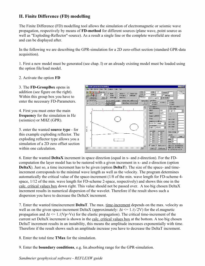
3. The FD-GroupBox opens inaddition (see figure on the right).Within this group box you have toenter the necessary FD-Parameters.

4. First you must enter the mainfrequency for the simulation in Hz(seismics) or MHZ (GPR).

5. enter the wanted source type - forthis example exploding reflector. Theexploding reflector type allows you asimulation of a 2D zero offset sectionwithin one calculation.

6. Enter the wanted DeltaX increment in space direction (equal in x- and z-direction). For the FD-computation the layer model has to be rastered with a given increment in x- and z-direction (optionDeltaX). Just so, a time increment has to be given (option DeltaT). The size of the space- and time-increment corresponds to the minimal wave length as well as the velocity. The program determinesautomatically the critical value of the space-increment (1/8 of the min. wave length for FD-scheme 4-space, 1/12 of the min. wave length for FD-scheme 2-space, respectively) and shows this one in thecalc. critical values box down right. This value should not be passed over. A too big chosen DeltaXincrement results in numerical dispersion of the wavelet. Therefore if the result shows such adispersion you have to decrease the DeltaX increment.

7. Enter the wanted timeincrement DeltaT. The max. time-increment depends on the max. velocity aswell as on the given space-increment DeltaX (approximately: ∆t <= 1./(%2V) for the el.magneticpropagation and ∆t <= 1./(Vp+Vs) for the elastic propagation). The critical time-increment of thecurrent set DeltaX increment is shown in the calc. critical values box at the bottom. A too big chosenDeltaT increment results in an instability, this means the amplitude increases exponentially with time.Therefore if the result shows such an amplitude increase you have to decrease the DeltaT increment.

8. Enter the total time TMax for the simulation.

9. Enter the boundary conditions, e.g. lin.absorbing range for the GPR-simulation.


10. Choose the wanted excitation and registration components. By default the EY-components areactivated.

11. Choose the output type - for this example single line.

12. Enter the output parameters for the single line (rec x start, rec x end, rec z start, rec z end). Forexample: rec x start: 0; rec x end: 5; rec z start: 0; rec z end: 0 (registration line at the surface)..

13. Activating the option StartFD starts first the rastering of model (if the option raster is activated)and then starts the external program FDEMSEIS.EXE which will normally be executed in thebackground (option background activated), so that it is possible to go on with the work in REFLEXW.If the option background is deselected, the computation is faster but there is no possibility to work withREFLEXW until the FD-computation is finished.

14. After having finished the FD-computation you may display the simulation result within the 2D-dataanalysis.


III. ray tracing

The ray tracing modelling tool allows the traveltime simulation of electromagnetic or seismic wavepropagation, respectively by means of a finite difference approximation of the eikonal equation. Thecalculation of the synthetic traveltimes is restricted to the first arrivals for an arbitrary 2-dimensionalmedium. No reflections and secondary arrivals can be calculated. This can be done using the FD-simulation (see chap. II). The main application is the seismic refraction but it is also possible to simulate any transmission data.The raytracing may be used for- the control of an inverted model- an iterative adaptation of the calculated and real data by stepwise changing the underground model

In the following the application to seismic refraction data is described. 1. first a new model must be generated (see chap. I) or an already existing model must be loaded usingthe option file/load model.

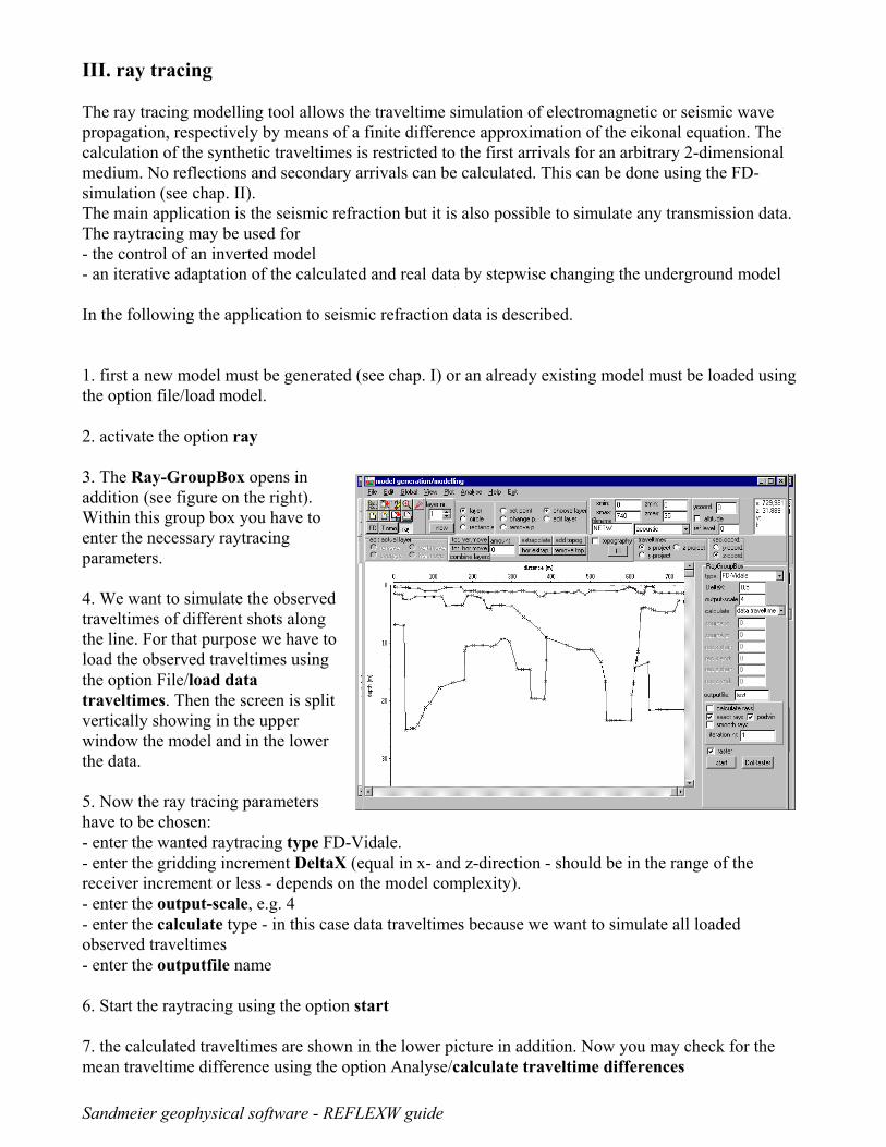
2. activate the option ray

3. The Ray-GroupBox opens inaddition (see figure on the right).Within this group box you have toenter the necessary raytracingparameters.

4. We want to simulate the observedtraveltimes of different shots alongthe line. For that purpose we have toload the observed traveltimes usingthe option File/load datatraveltimes. Then the screen is splitvertically showing in the upperwindow the model and in the lowerthe data.

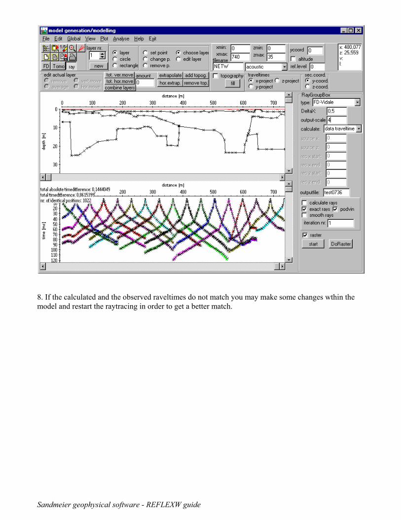
5. Now the ray tracing parametershave to be chosen: - enter the wanted raytracing type FD-Vidale.- enter the gridding increment DeltaX (equal in x- and z-direction - should be in the range of thereceiver increment or less - depends on the model complexity).- enter the output-scale, e.g. 4- enter the calculate type - in this case data traveltimes because we want to simulate all loadedobserved traveltimes- enter the outputfile name

6. Start the raytracing using the option start

7. the calculated traveltimes are shown in the lower picture in addition. Now you may check for themean traveltime difference using the option Analyse/calculate traveltime differences


8. If the calculated and the observed raveltimes do not match you may make some changes wthin themodel and restart the raytracing in order to get a better match.


IV. tomography

Tomographic methods have been well established for borehole-borehole or borehole-surfacemeasurements whereby the object will be directly transmitted (so called transmission tomography).

In the case of the 2D refraction vertical tomography all sources and receivers are located within oneline at the surface. In order to allow for a high data coverage within the medium vertical velocitygradients should be present and a curved raytracing for the calculation of the traveltimes must be used. REFLEXW supports a 2D- and 3D-transmission traveltime tomography and a 2D refractiontomography. For the 2D-tomography both straight and curved raytracing is supported. For the 3D-tomography only straight raytracing is supported.

Chapter IV.1 includes the format and the picking of the traveltime data.In chapter IV.2 the 2D tomographic interpretation of borehole-borehole transmission tomography isdescribed.In chapter IV.3 the 2D tomographic interpretation of a refraction tomography is described.

IV.1 picking the traveltime data and description of the format Before performing the tomography the traveltime data to be inverted must be present.

REFLEXW uses a 2D or 3D ASCII-data format:

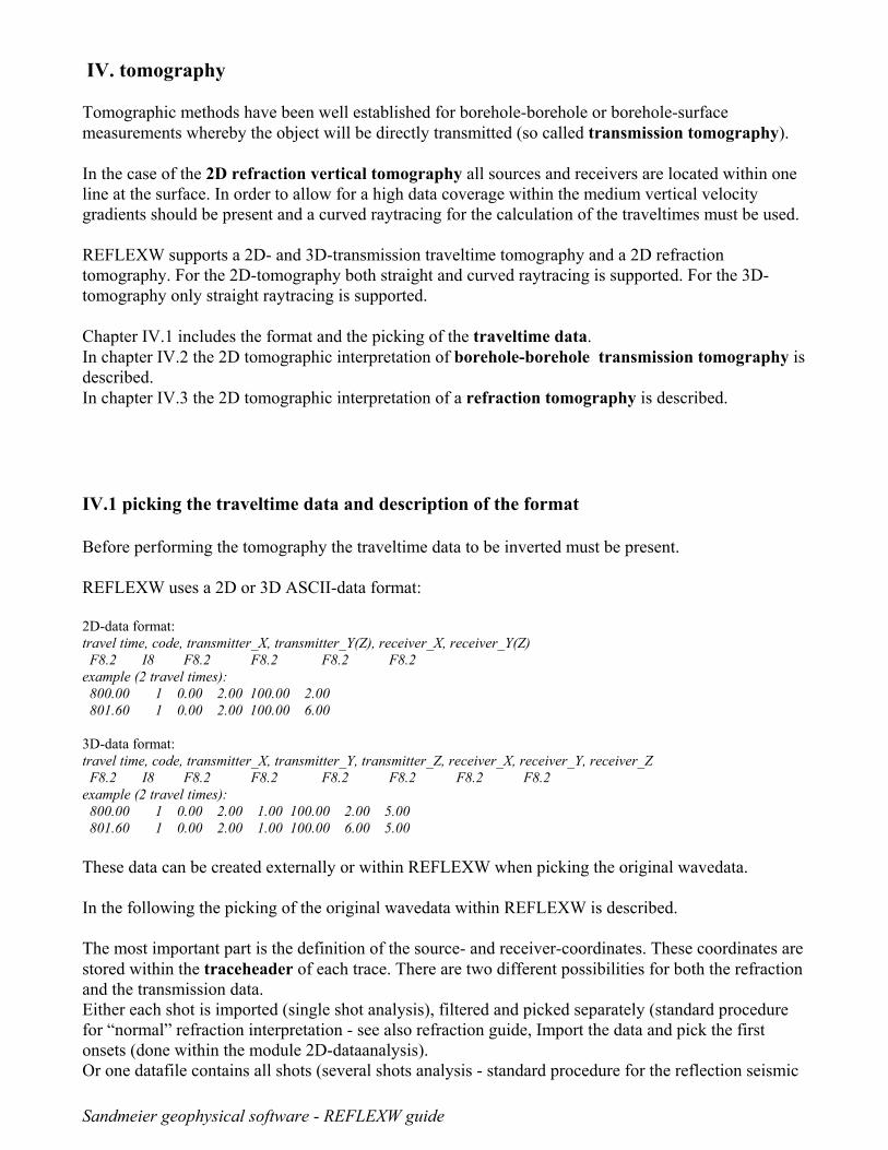
2D-data format:travel time, code, transmitter_X, transmitter_Y(Z), receiver_X, receiver_Y(Z) F8.2 I8 F8.2 F8.2 F8.2 F8.2example (2 travel times): 800.00 1 0.00 2.00 100.00 2.00 801.60 1 0.00 2.00 100.00 6.00

3D-data format: travel time, code, transmitter_X, transmitter_Y, transmitter_Z, receiver_X, receiver_Y, receiver_Z F8.2 I8 F8.2 F8.2 F8.2 F8.2 F8.2 F8.2example (2 travel times): 800.00 1 0.00 2.00 1.00 100.00 2.00 5.00 801.60 1 0.00 2.00 1.00 100.00 6.00 5.00

These data can be created externally or within REFLEXW when picking the original wavedata. In the following the picking of the original wavedata within REFLEXW is described.

The most important part is the definition of the source- and receiver-coordinates. These coordinates arestored within the traceheader of each trace. There are two different possibilities for both the refractionand the transmission data. Either each shot is imported (single shot analysis), filtered and picked separately (standard procedurefor “normal” refraction interpretation - see also refraction guide, Import the data and pick the firstonsets (done within the module 2D-dataanalysis). Or one datafile contains all shots (several shots analysis - standard procedure for the reflection seismic


interpretation - see also reflection guide, Import the data and setting the geometry (both done withinthe module 2D-dataanalysis) and the data are filtered and picked in one step. If a very high datacoverage is present the refraction data may also be handled like the reflection data with one datafilecontaining all shots. In that case the various possibilities of defining the geometry may be claimed.

To be considered: In any case the traceheader coordinates must be correctly defined before picking! Ifthe 2D-data format shall be used the x- and y-traceheadercoordinates will be considered. The z-traceheader coordinates will be ignored. In the following the definition for this 2D-data format forequidistant receivers will be described.


IV.1.1 single 2D shot analysis

Depending on the shot/receiver geometry three different data types can be distinguished:

single shot: surface/surface geometry - shots and receivers are located on the surface, e.g. seismicrefraction or reflection datasingle shot/boreholes: borehole/borehole geometry - shots and receivers are located within twoparallel boreholessingle shot/VSP: borehole/surface geometry - the receivers are location within a borehole, the shotsare located at the surface

The shotfiles can be imported and handled completely separately or using a conversion sequence.

IV.1.1.1 import each shotfile separately (conversion sequence set to no)

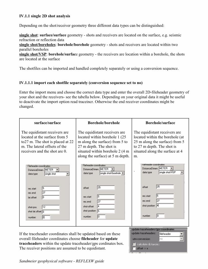
Enter the import menu and choose the correct data type and enter the overall 2D-fileheader geometry ofyour shot and the receivers- see the tabella below. Depending on your original data it might be usefulto deactivate the import option read traceincr. Otherwise the end receiver coordinates might bechanged.

surface/surface

The equidistant receivers arelocated at the surface from 5to27 m. The shot is placed at 22m. The lateral offsets of thereceivers and the shot are 0.

Borehole/borehole

The equidistant receivers arelocated within borehole 1 (25m along the surface) from 5 to27 m depth. The shot issituated within borehole 2 (4 malong the surface) at 5 m depth.

Borehole/surface

The equidistant receivers arelocated within the borehole (at25 m along the surface) from 5to 27 m depth. The shot issituated along the surface at 4m.

.

If the traceheader coordinates shall be updated based on theseoverall fileheader coordinates choose fileheader for updatetraceheaders within the update traceheader/gps cordinates box.The receiver positions are assumed to be equidistant.


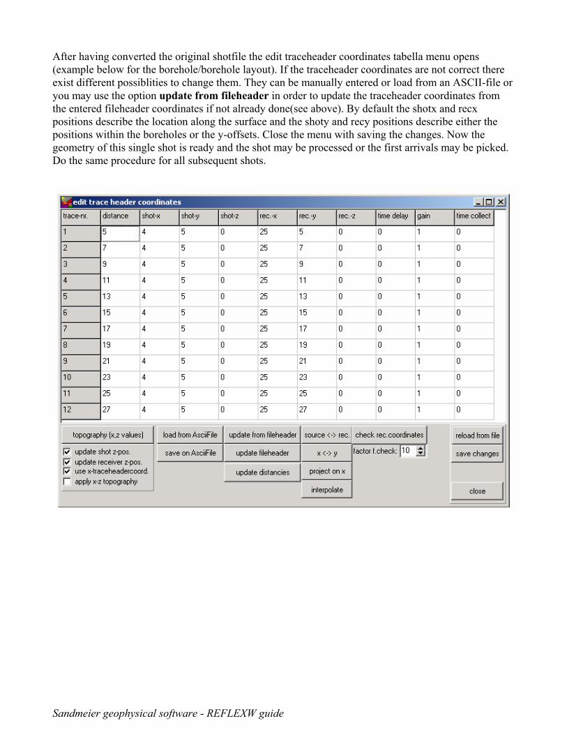
After having converted the original shotfile the edit traceheader coordinates tabella menu opens(example below for the borehole/borehole layout). If the traceheader coordinates are not correct thereexist different possiblities to change them. They can be manually entered or load from an ASCII-file oryou may use the option update from fileheader in order to update the traceheader coordinates fromthe entered fileheader coordinates if not already done(see above). By default the shotx and recxpositions describe the location along the surface and the shoty and recy positions describe either thepositions within the boreholes or the y-offsets. Close the menu with saving the changes. Now thegeometry of this single shot is ready and the shot may be processed or the first arrivals may be picked.Do the same procedure for all subsequent shots.


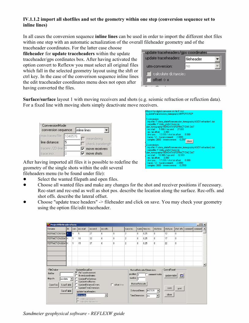
IV.1.1.2 import all shotfiles and set the geometry within one step (conversion sequence set toinline lines)

In all cases the conversion sequence inline lines can be used in order to import the different shot fileswithin one step with an automatic actualization of the overall fileheader geometry and of thetraceheader coordinates. For the latter case choosefileheader for update traceheaders within the updatetraceheader/gps cordinates box. After having activated theoption convert to Reflexw you must select all original fileswhich fall in the selected geometry layout using the shft orctrl key. In the case of the converison sequence inline linesthe edit traceheader coordinates menu does not open afterhaving converted the files.

Surface/surface layout 1 with moving receivers and shots (e.g. seismic refraction or reflection data).For a fixed line with moving shots simply deactivate move receivers.

After having imported all files it is possible to redefine thegeometry of the single shots within the edit severalfileheaders menu (to be found under file): ! Select the wanted filepath and open files.! Choose all wanted files and make any changes for the shot and receiver positions if necessary.

Rec-start and rec-end as well as shot pos. describe the location along the surface. Rec-offs. andshot offs. describe the lateral offset.

! Choose "update trace headers" -> fileheader and click on save. You may check your geometryusing the option file/edit traceheader.


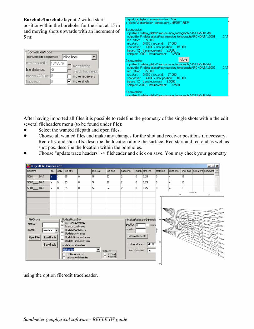
Borehole/borehole layout 2 with a startpositionwithin the borehole for the shot at 15 mand moving shots upwards with an increment of5 m:

After having imported all files it is possible to redefine the geometry of the single shots within the editseveral fileheaders menu (to be found under file): ! Select the wanted filepath and open files.! Choose all wanted files and make any changes for the shot and receiver positions if necessary.

Rec-offs. and shot offs. describe the location along the surface. Rec-start and rec-end as well asshot pos. describe the location within the boreholes.

! Choose "update trace headers" -> fileheader and click on save. You may check your geometry

using the option file/edit traceheader.


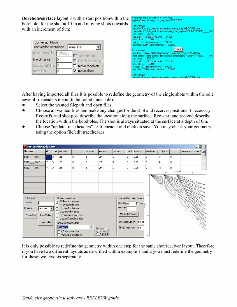
Borehole/surface layout 3 with a start positionwithin theborehole for the shot at 15 m and moving shots upwardswith an increment of 5 m:

After having imported all files it is possible to redefine the geometry of the single shots within the editseveral fileheaders menu (to be found under file): ! Select the wanted filepath and open files.! Choose all wanted files and make any changes for the shot and receiver positions if necessary.

Rec-offs. and shot pos. describe the location along the surface. Rec-start and rec-end describethe location within the boreholes. The shot is always situated at the surface at a depth of 0m.

! Choose "update trace headers" -> fileheader and click on save. You may check your geometryusing the option file/edit traceheader.

It is only possible to redefine the geometry within one step for the same shot/receiver layout. Thereforeif you have two different layouts as described within example 1 and 2 you must redefine the geometryfor these two layouts separately.


IV 1.2 several shots analysis

Putting all shots together has several advantages:- setting the geometry is easier- picking is faster

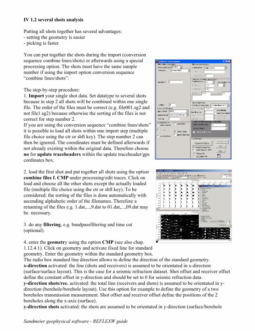
You can put together the shots during the import (conversionsequence combine lines/shots) or afterwards using a specialprocessing option. The shots must have the same samplenumber if using the import option conversion sequence“combine lines/shots”.

The step-by-step procedure:1. Import your single shot data. Set datatype to several shotsbecause in step 2 all shots will be combined within one singlefile. The order of the files must be correct (e.g. file001.sg2 andnot file1.sg2) because otherwise the sorting of the files is notcorrect for step number 2.If you are using the conversion sequence “combine lines/shots”it is possible to load all shots within one import step (multiplefile choice using the ctr or shft key). The step number 2 canthen be ignored. The coordinates must be defined afterwards ifnot already existing within the original data. Therefore chooseno for update traceheaders within the update traceheader/gpscordinates box.

2. load the first shot and put together all shots using the optioncombine files f. CMP under processing/edit traces. Click onload and choose all the other shots except the actually loadedfile (multiple file choice using the ctr or shft key). To beconsidered: the sorting of the files is done automatically withascending alphabetic order of the filenames. Therefore arenaming of the files e.g. 1.dat,...,9.dat to 01.dat,...,09.dat maybe necessary.

3. do any filtering, e.g. bandpassfiltering and time cut(optional).

4. enter the geometry using the option CMP (see also chap.1.12.4.1). Click on geometry and activate fixed line for standardgeometry. Enter the geometry within the standard geometry box.The radio box standard line direction allows to define the direction of the standard geometry. x-direction activated: the line (shots and receivers) is assumed to be orientated in x-direction(surface/surface layout). This is the case for a seismic refraction dataset. Shot offset and receiver offsetdefine the constant offset in y-direction and should be set to 0 for seismic refraction data.y-direction shots/rec. activated: the total line (receivers and shots) is assumed to be orientated in y-direction (borehole/borehole layout). Use this option for example to define the geometry of a twoboreholes transmission measurement. Shot offset and receiver offset define the positions of the 2boreholes along the x-axis (surface). y-direction shots activated: the shots are assumed to be orientated in y-direction (surface/borehole


layout). Use this option for example to define the geometry of a borehole containing the shots and thereceivers placed at the surface.Shotoffset specifies the x-position of the shot borehole and receiveroffset specifies the location of the receivers in y-direction (normally 0 for surface).y-direction rec. activated: the receivers are assumed to be orientated in y-direction (borehole/surfacelayout). Use this option for example to define the geometry of a borehole containing the receivers andthe shots placed at the surface. Receiver offset specifies the x-position of the receiver borehole and shotoffset specifies the location of the shots in y-direction (normally 0 for surface).Click on apply std. geometry - the geometry will be updated and save the geometry. It is recommendedto check the geometry of the individual traces using the edit single traces. The standard geometry must be applied separately on each individual configuration. A newconfiguration is given for example if the receiver line has been changed or if the shots and receivershave been exchanged. The parameters first trace and last trace define the range for the individualconfiguration. The following example is a dataset containing three different configurations corresponding to the threelayouts of chap. IV.1.1.

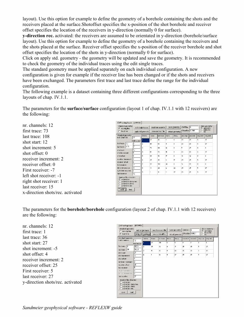
The parameters for the surface/surface configuration (layout 1 of chap. IV.1.1 with 12 receivers) arethe following:

nr. channels: 12first trace: 73last trace: 108shot start: 12shot increment: 5shot offset: 0receiver increment: 2receiver offset: 0First receiver: -7left shot receiver: -1right shot receiver: 1last receiver: 15x-direction shots/rec. activated

The parameters for the borehole/borehole configuration (layout 2 of chap. IV.1.1 with 12 receivers)are the following:

nr. channels: 12first trace: 1last trace: 36shot start: 27shot increment: -5shot offset: 4receiver increment: 2receiver offset: 25First receiver: 5last receiver: 27y-direction shots/rec. activated


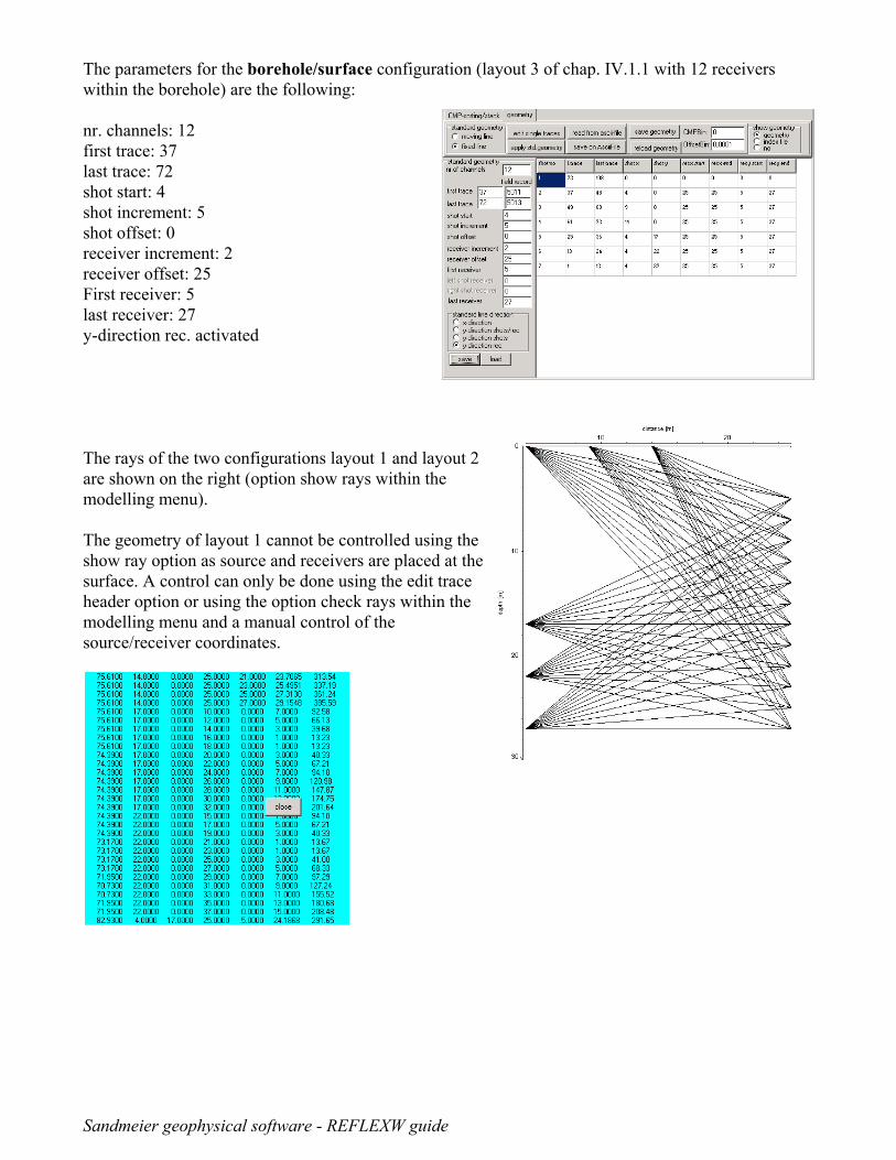
The parameters for the borehole/surface configuration (layout 3 of chap. IV.1.1 with 12 receiverswithin the borehole) are the following:

nr. channels: 12first trace: 37last trace: 72shot start: 4shot increment: 5shot offset: 0receiver increment: 2receiver offset: 25First receiver: 5last receiver: 27y-direction rec. activated

The rays of the two configurations layout 1 and layout 2are shown on the right (option show rays within themodelling menu).

The geometry of layout 1 cannot be controlled using theshow ray option as source and receivers are placed at thesurface. A control can only be done using the edit traceheader option or using the option check rays within themodelling menu and a manual control of thesource/receiver coordinates.


IV.1.3 picking the first arrivals

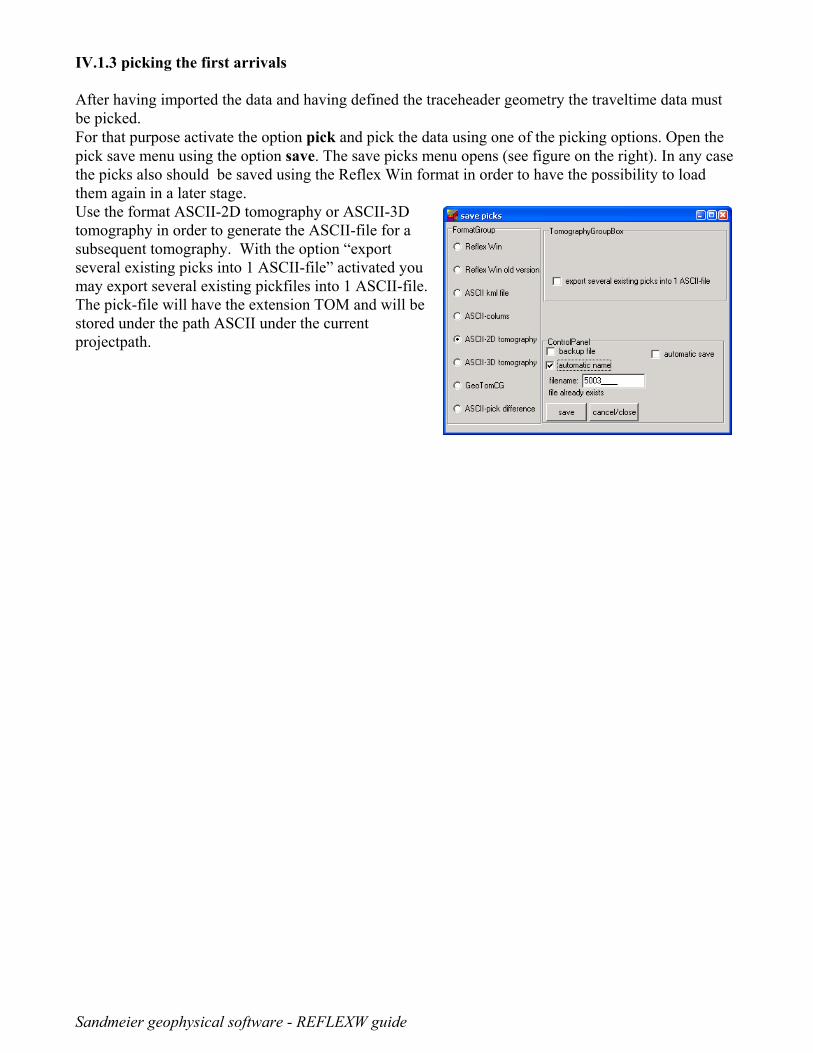
After having imported the data and having defined the traceheader geometry the traveltime data mustbe picked.For that purpose activate the option pick and pick the data using one of the picking options. Open thepick save menu using the option save. The save picks menu opens (see figure on the right). In any casethe picks also should be saved using the Reflex Win format in order to have the possibility to loadthem again in a later stage.Use the format ASCII-2D tomography or ASCII-3Dtomography in order to generate the ASCII-file for asubsequent tomography. With the option “exportseveral existing picks into 1 ASCII-file” activated youmay export several existing pickfiles into 1 ASCII-file.The pick-file will have the extension TOM and will bestored under the path ASCII under the currentprojectpath.


IV.2 performing the transmission tomography 1. First a starting model must be generated (see chap. I) or an already existing model must be loadedusing the option file/load model. Normally the starting model may be a simple homogeneous modelwhereby the velocity should be within the expected range.

2. Activate the option Tomo

3. The TomographyGroupBox opensin addition (see figure on the right).Within this group box you have toenter the necessary tomographyparameters.

- Load the data using the option loaddata (see also item 1). If the 3D-dataformat is used for the 2D-tomographyyou have to deactivate the option use2D-data and you have to specify thesecond coordinate (y or z) within theradiobox sec.coord. The firstcoordinate is always x. The thirdcoordinate is neglected.

- Check the geometry of your loaded traveltimedata using theoption show rays

- Enter the wanted space increment (equal in x- and z-direction).This increment should be within the range of the receiver or shotincrement.

- Activate the option curved ray if the curved raytracing shall beused. If activated the option start curved ray specifies theiteration step for which the curved raytracing will be used first. - For a first tomographic result you may use the other default parameters. There are no general rules forthese parameters but you have to adapt the parameters to your data in order to get the best result.

- Enter a name for the final model. Please use not the samename as for the starting model because this may lead toproblems.

- Start the tomography. The tomographic result is storedusing the “normal” REFLEXW format. You may display theresult within the 2D-dataanalysis.


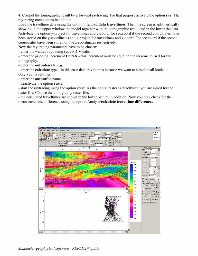
4. Control the tomographic result by a forward raytracing. For that purpose activate the option ray. Theraytracing menu opens in addition. Load the traveltime data using the option File/load data traveltimes. Then the screen is split verticallyshowing in the upper window the model together with the tomographic result and in the lower the data.Activbate the option y-project for traveltimes and y-coord. for sec.coord if the second coordinates havebeen stored on the y-coordinates and z-project for traveltimes and z-coord. For sec.coord if the secondcoordinates have been stored on the z-coordinates respectively.Now the ray tracing parameters have to be chosen: - enter the wanted raytracing type FD-Vidale.- enter the gridding increment DeltaX - this increment must be equal to the increment used for thetomography.- enter the output-scale, e.g. 1- enter the calculate type - in this case data traveltimes because we want to simulate all loadedobserved traveltimes- enter the outputfile name- deactivate the option raster - start the raytracing using the option start. As the option raster is deactivated you are asked for theraster file. Choose the tomography raster file. - the calculated traveltimes are shown in the lower picture in addition. Now you may check for themean traveltime difference using the option Analyse/calculate traveltime differences


IV.3 performing the refraction tomography

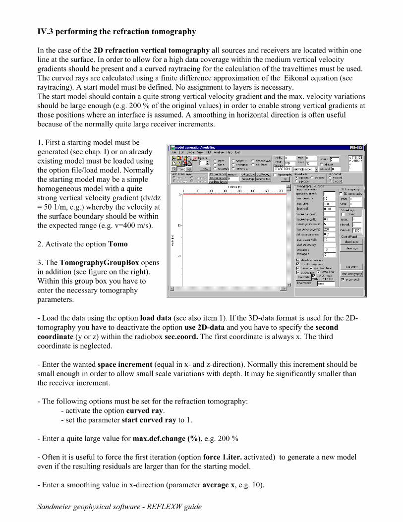
In the case of the 2D refraction vertical tomography all sources and receivers are located within oneline at the surface. In order to allow for a high data coverage within the medium vertical velocitygradients should be present and a curved raytracing for the calculation of the traveltimes must be used. The curved rays are calculated using a finite difference approximation of the Eikonal equation (seeraytracing). A start model must be defined. No assignment to layers is necessary.The start model should contain a quite strong vertical velocity gradient and the max. velocity variationsshould be large enough (e.g. 200 % of the original values) in order to enable strong vertical gradients atthose positions where an interface is assumed. A smoothing in horizontal direction is often usefulbecause of the normally quite large receiver increments. 1. First a starting model must begenerated (see chap. I) or an alreadyexisting model must be loaded usingthe option file/load model. Normallythe starting model may be a simplehomogeneous model with a quitestrong vertical velocity gradient (dv/dz= 50 1/m, e.g.) whereby the velocity atthe surface boundary should be withinthe expected range (e.g. v=400 m/s).

2. Activate the option Tomo

3. The TomographyGroupBox opensin addition (see figure on the right).Within this group box you have toenter the necessary tomographyparameters.

- Load the data using the option load data (see also item 1). If the 3D-data format is used for the 2D-tomography you have to deactivate the option use 2D-data and you have to specify the secondcoordinate (y or z) within the radiobox sec.coord. The first coordinate is always x. The thirdcoordinate is neglected.

- Enter the wanted space increment (equal in x- and z-direction). Normally this increment should besmall enough in order to allow small scale variations with depth. It may be significantly smaller thanthe receiver increment.

- The following options must be set for the refraction tomography:- activate the option curved ray. - set the parameter start curved ray to 1.

- Enter a quite large value for max.def.change (%), e.g. 200 %

- Often it is useful to force the first iteration (option force 1.iter. activated) to generate a new modeleven if the resulting residuals are larger than for the starting model.

- Enter a smoothing value in x-direction (parameter average x, e.g. 10).


- Activate the option show result in order to display the tomography result

- For a first tomographic result you may use the other default parameters. There are no general rulesfor these parameters but you have to adapt the parameters to your data in order to get the best result.

- Enter a name for the final model. Note: do not use the same name like for the starting model.

- Start the tomography. The tomographic result is stored using the “normal” REFLEXW format. Youmay display the result within the 2D-dataanalysis.

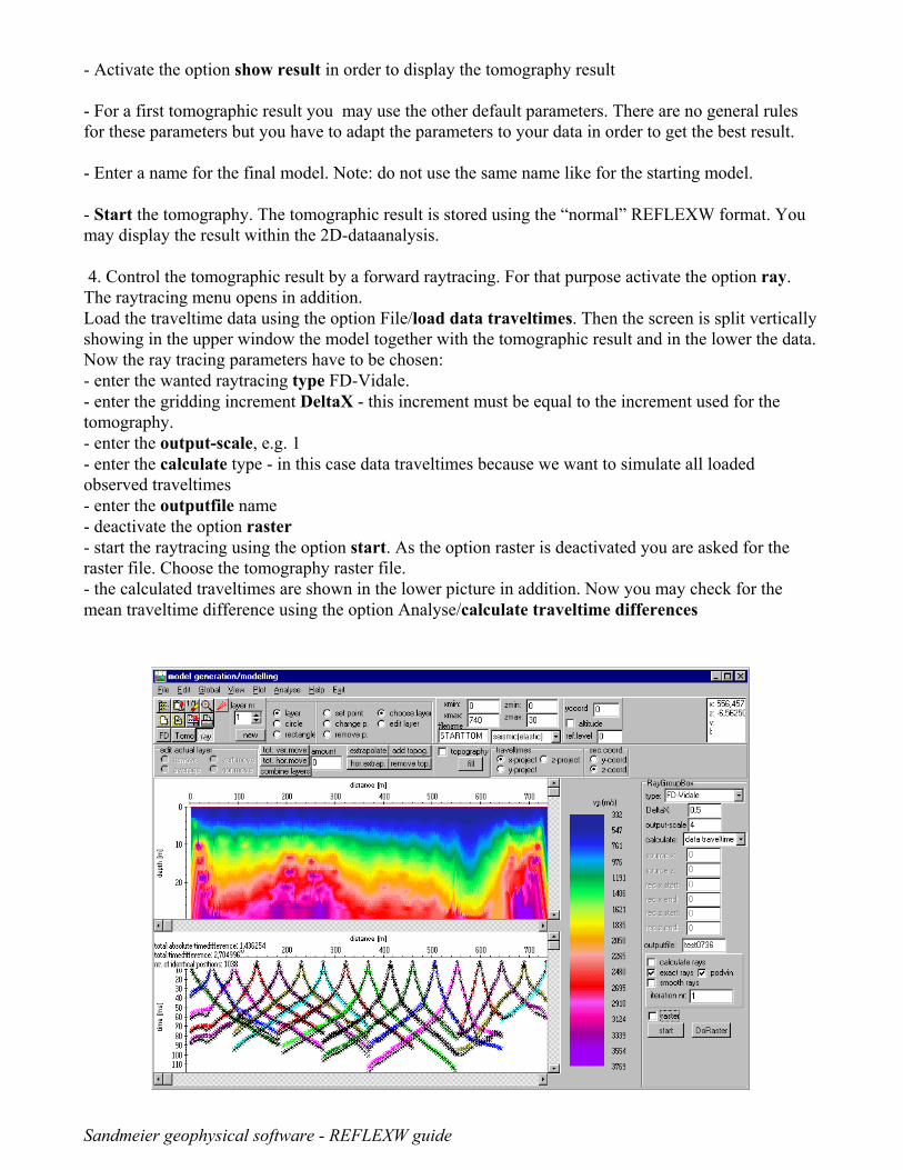
4. Control the tomographic result by a forward raytracing. For that purpose activate the option ray.The raytracing menu opens in addition. Load the traveltime data using the option File/load data traveltimes. Then the screen is split verticallyshowing in the upper window the model together with the tomographic result and in the lower the data. Now the ray tracing parameters have to be chosen: - enter the wanted raytracing type FD-Vidale.- enter the gridding increment DeltaX - this increment must be equal to the increment used for thetomography.- enter the output-scale, e.g. 1- enter the calculate type - in this case data traveltimes because we want to simulate all loadedobserved traveltimes- enter the outputfile name- deactivate the option raster - start the raytracing using the option start. As the option raster is deactivated you are asked for theraster file. Choose the tomography raster file. - the calculated traveltimes are shown in the lower picture in addition. Now you may check for themean traveltime difference using the option Analyse/calculate traveltime differences

Documents

Introduction to the modelling/tomography tools within ... like described under step 6. 9. Return to the main modelling menu by simply ... Therefore the program searches automatically