Introduction to the Maxwell Garnett approximation: tutorial · Introduction to the Maxwell Garnett approximation: tutorial ... This tutorial is devoted to the Maxwell Garnett

Introduction to the Maxwell Garnettapproximation: tutorialVADIM A. MARKEL1,2

1Aix-Marseille Université, CNRS, Centrale Marseille, Institut Fresnel UMR 7249, 13013 Marseille, France ([email protected])2On leave from Department of Radiology, University of Pennsylvania, Philadelphia, Pennsylvania 19104, USA ([email protected])

Received 29 February 2016; revised 21 April 2016; accepted 24 April 2016; posted 28 April 2016 (Doc. ID 260083); published 6 June 2016

This tutorial is devoted to the Maxwell Garnett approximation and related theories. Topics covered in this first,introductory part of the tutorial include the Lorentz local field correction, the Clausius–Mossotti relation andits role in the modern numerical technique known as the discrete dipole approximation, the Maxwell Garnettmixing formula for isotropic and anisotropic media, multicomponent mixtures and the Bruggeman equation, theconcept of smooth field, and Wiener and Bergman–Milton bounds. © 2016 Optical Society of America

OCIS codes: (000.1600) Classical and quantum physics; (160.0160) Materials.

http://dx.doi.org/10.1364/JOSAA.33.001244

1. INTRODUCTION

In 1904, Maxwell Garnett developed a simple but immenselysuccessful homogenization theory [1,2]. As any such theory, it aimsto approximate a complex electromagnetic medium such as acolloidal solution of gold microparticles in water with a homo-geneous effective medium. The Maxwell Garnett mixing formulagives the permittivity of this effective medium (or, simply, theeffective permittivity) in terms of the permittivities and volumefractions of the individual constituents of the complex medium.

A closely related development is the Lorentz molecular theoryof polarization. This theory considers a seemingly differentphysical system: a collection of point-like polarizable atoms ormolecules in vacuum. The goal is, however, the same: computethe macroscopic dielectric permittivity of the medium made upby this collection of molecules. A key theoretical ingredient ofthe Lorentz theory is the so-called local field correction, and thisingredient is also used in the Maxwell Garnett theory.

The two theories mentioned above seem to start from verydifferent first principles. The Maxwell Garnett theory startsfrom the macroscopic Maxwell’s equations, which are assumedto be valid on a fine scale inside the composite. The Lorentztheory does not assume that the macroscopic Maxwell’s equa-tions are valid locally. The molecules cannot be characterized bymacroscopic quantities such as permittivity, contrary to smallinclusions in a composite. However, the Lorentz theory is stillmacroscopic in nature. It simply replaces the description ofinclusions in terms of the internal field and polarization bya cumulative characteristic called the polarizability. Within theapproximations used by both theories, the two approaches aremathematically equivalent.

An important point is that we should not confuse the the-ories of homogenization that operate with purely classical and

macroscopic quantities with the theories that derive the macro-scopic Maxwell’s equations (and the relevant constitutiveparameters) from microscopic first principles, which are in thiscase the microscopic Maxwell’s equations and the quantum-mechanical laws of motion. Both the Maxwell Garnett andLorentz theories are of the first kind. An example of the secondkind is the modern theory of polarization [3,4], which com-putes the induced microscopic currents in a condensedmedium (this quantity turns out to be fundamental) by usingthe density-functional theory (DFT).

This tutorial will consist of two parts. In the first, introduc-tory part, we will discuss the Maxwell Garnett and Lorentztheories and the closely related Clausius–Mossotti relation fromthe same simple theoretical viewpoint. We will not attempt togive an accurate historical overview or to compile an exhaustivelist of references. It would also be rather pointless to write downthe widely known formulas and make several plots for modelsystems. Rather, we will discuss the fundamental underpin-nings of these theories. In the second part, we will discussseveral advanced topics that are rarely covered in the textbooks.We will then sketch a method for obtaining more generalhomogenization theories in which the Maxwell Garnett mixingformula serves as the zeroth-order approximation.

Over the past hundred years or so, the Maxwell Garnettapproximation and its generalizations have been derived bymany authors using different methods. It is unrealistic to coverall these approaches and theories in this tutorial. Therefore, wewill make an unfortunate compromise and not discuss someimportant topics. One notable omission is that we will not dis-cuss random media [5–7] in any detail, although the first partof the tutorial will apply equally to both random and determin-istic (periodic) media. Another interesting development that

1244 Vol. 33, No. 7 / July 2016 / Journal of the Optical Society of America A Tutorial

1084-7529/16/071244-13 Journal © 2016 Optical Society of America

mailto:[email protected]






http://dx.doi.org/10.1364/JOSAA.33.001244

we will not discuss is the so-called extended Maxwell Garnetttheories [8–10] in which the inclusions are allowed to haveboth electric and magnetic dipole moments.

A Gaussian system of units will be used throughout thetutorial.

2. LORENTZ LOCAL FIELD CORRECTION,CLAUSIUS–MOSSOTTI RELATION, ANDMAXWELL GARNETT MIXING FORMULA

The Maxwell Garnett mixing formula can be derived by differ-ent methods, some being more formal than others. We willstart by introducing the Lorentz local field correction andderiving the Clausius–Mossotti relation. The Maxwell Garnettmixing formula will follow from these results quite naturally.We emphasize, however, that this is not how the theory hasprogressed historically.

A. Average Field of a Dipole

The key mathematical observation that we will need is this: Theintegral over any finite sphere of the electric field created by astatic point dipole d located at the sphere’s center is not zero butequal to −�4π∕3�d.

The above statement may appear counterintuitive to anyonewho has seen the formula for the electric field of a dipole,

Ed�r� �3r̂�r̂ · d� − d

r3; (1)

where r̂ � r∕r is the unit vector pointing in the direction of theradius vector r. Indeed, the angular average of the above expres-sion is zero [11]. Nevertheless, the statement made above iscorrect. The reason is that the expression (1) is incomplete. Weshould have written

Ed�r� �3r̂�r̂ · d� − d

r3−4π

3δ�r�d; (2)

where δ�r� is the three-dimensional Dirac delta function.The additional delta term in Eq. (2) can be understood from

many different points of view. Three explanations of varyingdegree of mathematical rigor are given below.

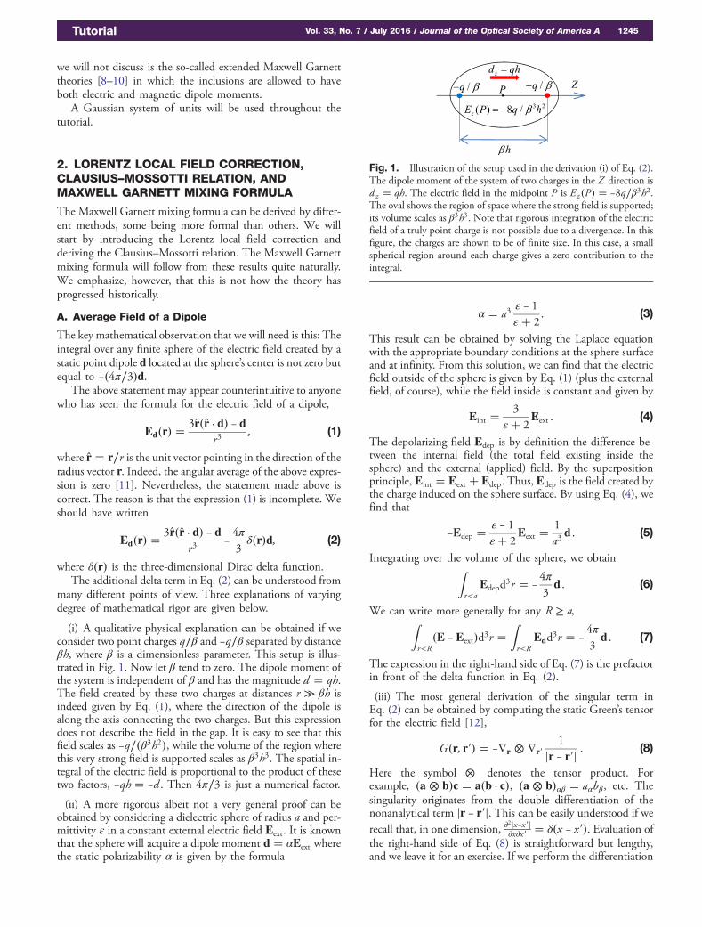
(i) A qualitative physical explanation can be obtained if weconsider two point charges q∕β and −q∕β separated by distanceβh, where β is a dimensionless parameter. This setup is illus-trated in Fig. 1. Now let β tend to zero. The dipole moment ofthe system is independent of β and has the magnitude d � qh.The field created by these two charges at distances r ≫ βh isindeed given by Eq. (1), where the direction of the dipole isalong the axis connecting the two charges. But this expressiondoes not describe the field in the gap. It is easy to see that thisfield scales as −q∕�β3h2�, while the volume of the region wherethis very strong field is supported scales as β3h3. The spatial in-tegral of the electric field is proportional to the product of thesetwo factors, −qh � −d . Then 4π∕3 is just a numerical factor.

(ii) A more rigorous albeit not a very general proof can beobtained by considering a dielectric sphere of radius a and per-mittivity ε in a constant external electric field Eext. It is knownthat the sphere will acquire a dipole moment d � αEext wherethe static polarizability α is given by the formula

α � a3ε − 1

ε� 2: (3)

This result can be obtained by solving the Laplace equationwith the appropriate boundary conditions at the sphere surfaceand at infinity. From this solution, we can find that the electricfield outside of the sphere is given by Eq. (1) (plus the externalfield, of course), while the field inside is constant and given by

Eint �3

ε� 2Eext : (4)

The depolarizing field Edep is by definition the difference be-tween the internal field (the total field existing inside thesphere) and the external (applied) field. By the superpositionprinciple, Eint � Eext � Edep. Thus, Edep is the field created bythe charge induced on the sphere surface. By using Eq. (4), wefind that

−Edep �ε − 1

ε� 2Eext �

1

a3d : (5)

Integrating over the volume of the sphere, we obtainZr<a

Edepd3r � −

4π

3d : (6)

We can write more generally for any R ≥ a,Zr<R

�E − Eext�d3r �Zr<R

Edd3r � −

4π

3d : (7)

The expression in the right-hand side of Eq. (7) is the prefactorin front of the delta function in Eq. (2).

(iii) The most general derivation of the singular term inEq. (2) can be obtained by computing the static Green’s tensorfor the electric field [12],

G�r; r 0� � −∇r ⊗ ∇r 01

jr − r 0j : (8)

Here the symbol ⊗ denotes the tensor product. Forexample, �a ⊗ b�c � a�b · c�, �a ⊗ b�αβ � aαbβ, etc. Thesingularity originates from the double differentiation of thenonanalytical term jr − r 0j. This can be easily understood if werecall that, in one dimension, ∂

2jx−x 0 j∂x∂x 0 � δ�x − x 0�. Evaluation of

the right-hand side of Eq. (8) is straightforward but lengthy,and we leave it for an exercise. If we perform the differentiation

Fig. 1. Illustration of the setup used in the derivation (i) of Eq. (2).The dipole moment of the system of two charges in the Z direction isdz � qh. The electric field in the midpoint P is Ez�P� � −8q∕β3h2.The oval shows the region of space where the strong field is supported;its volume scales as β3h3. Note that rigorous integration of the electricfield of a truly point charge is not possible due to a divergence. In thisfigure, the charges are shown to be of finite size. In this case, a smallspherical region around each charge gives a zero contribution to theintegral.

Tutorial Vol. 33, No. 7 / July 2016 / Journal of the Optical Society of America A 1245

accurately and then set r 0 � 0, we will find that G�r; 0�d isidentical to the right-hand side of Eq. (2).

Now, the key approximation of the Lorentz moleculartheory of polarization, as well as that of the Maxwell Garnetttheory of composites, is that the regular part in the right-handside of Eq. (2) averages to zero and, therefore, it can be ignored,whereas the singular part does not average to zero and shouldbe retained. We will now proceed with applying this idea to aphysical problem.

B. Lorentz Local Field Correction

Consider some spatial region V of volume V containingN ≫ 1 small particles of polarizability α each. We can referto the particles as “molecules.” The only important physicalproperty of a molecule is that it has a linear polarizability.The specific volume per one molecule is v � V ∕N . We willfurther assume that V is connected and sufficiently “simple.”For example, we can consider a plane-parallel layer or a sphere.In these two cases, the macroscopic electric field inside themedium is constant, which is important for the arguments pre-sented below. The system under consideration is schematicallyillustrated in Fig. 2.

Let us now place the whole system in a constant externalelectric field Eext. We will neglect the electromagnetic interactionof all the dipoles since we have decided to neglect the regular partof the dipole field in Eq. (2). Again, the assumption that we use isthat this field is unimportant because it averages to zero whensummed over all dipoles. In this case, each dipole “feels” theexternal field Eext, and therefore it acquires the dipole momentd � αEext. The total dipole moment of the object is

dtot � Nd � NαEext : (9)

On the other hand, if we assign the sample some macroscopicpermittivity ε and polarization P � ��ε − 1�∕4π�E, then the totaldipole moment is given by

dtot � V P � Vε − 1

4πE : (10)

In the above expression, E is the macroscopic electric field insidethe medium, which is, of course, different from theapplied field Eext. To find the relation between the two fields,we can use the superposition principle and write

E � Eext ��X

nEn�r�

�; r ∈ V : (11)

Here En�r� is the field produced by the n-th dipole, and h…idenotes averaging over the volume of the sample. Of course, theindividual fields En�r� will fluctuate and so will the sum of allthese contributions,

PnEn�r�. The averaging in the right-hand

side of Eq. (11) has been introduced since we believe that themacroscopic electric field is a suitably defined average of thefast-fluctuating “microscopic” field.

We now compute the averages in Eq. (11) as follows:

hEn�r�i �1

V

ZVEd�r − rn�d3r ≈ −

4π

3

dV; (12)

where rn is the location of the n-th dipole and Ed�r� is given byEq. (2). In performing the integration, we have disregarded theregular part of the dipole field, and, therefore, the second equal-ity above is approximate. We now substitute Eq. (12) intoEq. (11) and obtain the following result:

E � Eext �Xn

hEni � Eext − N4π

3

dV

��1 −

4π

3

α

v

�Eext :

(13)

In the above chain of equalities, we have used d � αEext

and V ∕N � v.All that is left to do now is substitute Eq. (13) into Eq. (10)

and use the condition that Eqs. (9) and (10) must yield thesame total dipole moment of the sample. Equating the right-hand sides of these two equations and dividing by the total vol-ume V results in the equation

α

v� ε − 1

4π

�1 −

4π

3

α

v

�: (14)

We now solve this equation for ε and obtain

ε � 1� 4π�α∕v�1 − �4π∕3��α∕v� �

1� �8π∕3��α∕v�1 − �4π∕3��α∕v� : (15)

This is the Lorentz formula for the permittivity of a nonpolarmolecular gas. The denominator in Eq. (15) accounts for thefamous local field correction. The external field Eext is fre-quently called the local field and denoted by EL.Equation (13) is the linear relation between the local field andthe average macroscopic field.

If we did not know about the local field correction, we couldhave written naively ε � 1� 4π�α∕v�. Of course, in dilutegases, the denominator in Eq. (15) is not much different fromunity. To first order in α∕v, the above (incorrect) formula andEq. (15) are identical. The differences show up only to secondorder in α∕v. The significance of higher-order terms in the ex-pansion of ε in powers of α∕v and the applicability range of theLorentz formula can be evaluated only by constructing a morerigorous theory from which Eq. (15) is obtained as a limit. Herewe can mention that, in the case of dilute gases, the local fieldcorrection plays a more important role in nonlinear optics,where field fluctuations can be enhanced by the nonlinearities.Also, in some applications of the theory involving linear opticsof condensed matter (with ε substantially different from unity),the exact form of the denominator in Eq. (15) turns out to beimportant. An example will be given in Section 2.C below.

Fig. 2. Collection of dipoles in an external field. The particles aredistributed inside a spherical volume either randomly (as shown) orperiodically. It is assumed, however, that the macroscopic densityof particles is constant inside the sphere and equal to v−1 � N∕V .Here v is the specific volume per one particle.


It is interesting to note that we have derived the local fieldcorrection without the usual trick of defining the Lorentzsphere and assuming that the medium outside of this sphereis truly continuous, etc. The approaches are, however, math-ematically equivalent if we get to the bottom of what is goingon in the Lorentz molecular theory of polarization. The deri-vation shown above illustrates one important but frequentlyoverlooked fact, namely, that the mathematical nature of theapproximation made by the Lorentz theory is very simple: itis to disregard the regular part of the expression (2). Onecan state the approximation mathematically by writingEd�r� � −�4π∕3�δ�r�d instead of Eq. (2). No other approxi-mation or assumption is needed.

C. Clausius–Mossotti Relation

Instead of expressing ε in terms of α∕v, we can express α∕v interms of ε. Physically, the question that one might ask is this.Let us assume that we know ε of some medium (say, it wasmeasured) and know that it is describable by the Lorentz for-mula. Then what is the value of α∕v for the molecules thatmake up this medium? The answer can be easily found fromEq. (14), and it reads

α

v� 3

4π

ε − 1

ε� 2: (16)

This equation is known as the Clausius–Mossotti relation.It may seem that Eq. (16) does not contain any new infor-

mation compared to Eq. (15). Mathematically this is indeed sobecause one equation follows from the other. However, in 1973,Purcell and Pennypacker proposed a numerical method for solv-ing boundary-value electromagnetic problems for macroscopicparticles of arbitrary shape [13] that is based on a somewhatnontrivial application of the Clausius–Mossotti relation.

The main idea of this method is as follows. We know thatEq. (16) is an approximation. However, we expect Eq. (16) tobecome accurate in the limit a∕h → 0, where h � v1∕3 is thecharacteristic interparticle distance and a is the characteristicsize of the particles. Physically, this limit is not interesting be-cause it leads to the trivial results α∕v → 0 and ε → 1. But thisis true for physical particles. What if we consider hypotheticalpoint-like particles and assign to them the polarizability thatfollows from Eq. (16) with some experimental value of ε? Itturns out that an array of such hypothetical point dipoles ar-ranged on a cubic lattice and constrained to the overall shape ofthe sample mimics the electromagnetic response of the latterwith arbitrarily good precision as long as the macroscopic fieldin the sample does not vary significantly on the scale of h (so hshould be sufficiently small). We, therefore, can replace theactual sample by an array of N point dipoles. The electromag-netic problem is then reduced to solvingN linear coupled-dipoleequations, and the corresponding method is known as the dis-crete dipole approximation (DDA) [14].

One important feature of DDA is that, for the purpose ofsolving the coupled-dipole equations, one should not disregardthe regular part of Eq. (2). This is in spite of the fact that wehave used this assumption to arrive at Eq. (16) in the firstplace. This might seem confusing, but there is really no contra-diction because DDA can be derived from more general con-siderations than what was used above. Originally, it was derived

by discretizing the macroscopic Maxwell’s equations written inthe integral form [13]. The reason why the regular part ofEq. (2) must be retained in the coupled-dipole equations is be-cause we are interested in samples of arbitrary shape, and theregular part of Eq. (2) does not really average out to zero in thiscase. Moreover, we can apply DDA beyond the static limit,where no such cancellation takes place in principle. Of course,the expression for the dipole field [Eq. (2)] and the Clausius–Mossotti relation [Eq. (16)] must be modified beyond the staticlimit to take into account the effects of retardation, the radiativecorrection to the polarizability, and other corrections associatedwith the finite frequency [15]—otherwise, the method will vi-olate energy conservation and can produce other abnormalities.

We note, however, that if we attempt to apply DDA to thestatic problem of a dielectric sphere in a constant external field,we will obtain the correct result from DDA either with or with-out account for the point–dipole interaction. In other words, ifwe represent a dielectric sphere of radius R and permittivity εby a large number N of point dipoles uniformly distributedinside the sphere and characterized by the polarizability givenin Eq. (16), subject all these dipoles to an external field, andsolve the arising coupled-dipole equations, we will recover thecorrect result for the total dipole moment of the large sphere.We can obtain this result without accounting for the interac-tion of the point dipoles. This can be shown by observing thatthe polarizability of the large sphere, αtot, is equal to Nα, whereα is given by Eq. (16). Alternatively, we can solve the coupled-dipole equations with the full account of dipole–dipoleinteraction on a supercomputer and—quite amazingly—wewill obtain the same result. This is so because the regular partsof the dipole fields, indeed, cancel out in this particular geom-etry (as long as N → ∞, of course). This simple observationunderscores the very deep theoretical insight of the Lorentzand Maxwell Garnett theories.

We also note that, in the context of DDA, the Lorentzlocal field correction is really important. Previously, we haveremarked that this correction is not very important fordilute gases. But if we started from the “naive” formulaε � 1� 4π�α∕v�, we would have gotten the incorrect“Clausius–Mossotti” relation of the form α∕v � �ε − 1�∕4πand, with this definition of α∕v, DDA would definitely notwork even in the simplest geometries.

To conclude the discussion of DDA, we would like toemphasize one important but frequently overlooked fact.Namely, the point dipoles used in DDA do not correspond toany physical particles. Their normalized polarizabilities α∕v arecomputed from the actual ε of material, which can be signifi-cantly different from unity. Yet the size of these dipoles is as-sumed to be vanishingly small. In this respect, DDA is verydifferent from the Foldy–Lax approximation [16,17], whichis known in the physics literature as, simply, the dipoleapproximation (DA) and which describes the electromagneticinteraction of sufficiently small physical particles via the dipoleradiation fields. The coupled-dipole equations are, however,formally the same in both DA and DDA.

The Clausius–Mossotti relation and the associated coupled-dipole equation (this time, applied to physical molecules)have also been used to study the fascinating phenomenon of


ferroelectricity (spontaneous polarization) of nanocrystals [18],the surface effects in organic molecular films [19], and manyother phenomena wherein the dipole interaction of moleculesor particles captures the essential physics.

D. Maxwell Garnett Mixing Formula

We are now ready to derive the Maxwell Garnett mixingformula. We will start with the simple case of small sphericalparticles in vacuum. This case is conceptually very close to theLorentz molecular theory of polarization. Of course, the latteroperates with “molecules,” but the only important physicalcharacteristic of a molecule is its polarizability, α. A small in-clusion in a composite can also be characterized by its polar-izability. Therefore, the two models are almost identical.

Consider spherical particles of radius a and permittivity εthat are distributed in vacuum either on a lattice or randomlybut uniformly on average. The specific volume per one particleis v, and the volume fraction of inclusions is f � �4π∕3��a3∕v�. The effective permittivity of such a medium can becomputed by applying Eq. (15) directly. The only thing thatwe will do is substitute the appropriate expression for α, whichin the case considered is given by Eq. (3). We then have

εMG �1� 2f

ε − 1

ε� 2

1 − fε − 1

ε� 2

�1� 1� 2f

3�ε − 1�

1� 1 − f3

�ε − 1�: (17)

This is the Maxwell Garnett mixing formula (hence thesubscript MG) for small inclusions in vacuum. We emphasizethat, unlike in the Lorentz theory of polarization, εMG is theeffective permittivity of a composite, not the usual permittivityof a natural material.

Next, we remove the assumption that the backgroundmedium is vacuum, which is not realistic for composites. Letthe host medium have the permittivity εh and the inclusionshave the permittivity εi. The volume fraction of inclusions isstill equal to f . We can obtain the required generalizationby making the substitutions εMG → εMG∕εh and ε → εi∕εh,which yields

εMG� εh

1�2fεi −εhεi�2εh

1−fεi −εhεi�2εh

� εhεh�

1�2f3

�εi −εh�

εh�1−f3

�εi −εh�: (18)

We will now justify this result mathematically by tracing thesteps that were made to derive Eq. (17) and making appropriatemodifications.

We first note that the expression (2) for a dipole embeddedin an infinite host medium [20] should be modified as

Ed�r� �1

εh

�3r̂�r̂ · d� − d

r3−4π

3δ�r�d

�: (19)

This can be shown by using the equation ∇ · D �εh∇ · E � 4πρ, where ρ is the density of the electric chargemaking up the dipole. However, this argument may not be veryconvincing because it is not clear what is the exact nature of thecharge ρ and how it follows from the constitutive relations inthe medium. Therefore, we will now consider the argument(ii) given in Section 2.A and adjust it to the case of a spherical

inclusion of permittivity εi in a host medium of permittivity εh.The polarization field in this medium can be decomposed intotwo contributions, P � Ph � Pi, where

Ph�r� �εh − 1

4πE�r�; Pi�r� �

ε�r� − εh4π

E�r�: (20)

Obviously, Pi�r� is identically zero in the host medium whilePh�r� can be nonzero anywhere. The polarization Pi�r� is thesecondary source of the scattered field. To see that this is the case,we can start from the equation ∇ · ε�r�E�r� � 0 and write

∇ · εhE�r� � −∇ · �ε�r� − εh�E�r� � 4πρi�r�;where ρi � −∇ · Pi (note that the total induced charge is ρ �ρi � ρh, ρh � −∇ · Ph). Therefore, the relevant dipole momentof a spherical inclusion of radius a is d � R

r<a Pid3r. The

corresponding polarizability α and the depolarizing field insidethe inclusion Edep can be found by solving the Laplace equationfor a sphere embedded in an infinite host and are given by

α � a3εhεi − εhεi � 2εh

�compare to �3�� ; (21a)

−Edep �εi − εhεi � 2εh

Eext �d

εha3�compare to �5�� : (21b)

We thus find that the generalization of Eq. (7) to a mediumwith a nonvacuum host isZ

r<R�E − Eext�d3r �

Zr<R

Edd3r � −

4π

3εhd: (22)

Correspondingly, the formula relating the external and the aver-age fields (Lorentz local field correction) now reads

E ��1 −

4π

3εh

α

v

�Eext; (23)

where α is given by Eq. (21a). We now consider a spatialregion V that contains many inclusions and compute its totaldipole moment by two formulas: dtot � NαEext and dtot �V ��εMG − εh�∕4π�E. Equating the right-hand sides of thesetwo expressions and substituting E in terms of Eext fromEq. (23), we obtain the result

εMG � εh �4π�α∕v�

1 − �4π∕3εh��α∕v�: (24)

Substituting α from Eq. (21a) and using 4πa3∕3v � f , we ob-tain Eq. (18). As expected, one power of εh cancels in the de-nominator of the second term in the right-hand side of Eq. (24)but not in its numerator.

Finally, we make one conceptually important step, whichwill allow us to apply the Maxwell Garnett mixing formulato a much wider class of composites. Equation (18) was derivedunder the assumption that the inclusions are spherical. ButEq. (18) does not contain any information about the inclusionsshape. It only contains the permittivities of the host and theinclusions and the volume fraction of the latter. We thereforemake the conjecture that Eq. (18) is a valid approximationfor inclusions of any shape as long as the medium is spatiallyuniform and isotropic on average. Making this conjecture nowrequires some leap of faith, but a more solid justification willbe given in the second part of this tutorial.


3. MULTICOMPONENT MIXTURES AND THEBRUGGEMAN MIXING FORMULA

Equation (18) can be rewritten in the following form:εMG − εhεMG � 2εh

� fεn − εhεn � 2εh

; (25)

Let us now assume that the medium contains inclusions madeof different materials with permittivities εn (n � 1; 2;…; N ).Then Eq. (25) is generalized as

εMG − εhεMG � 2εh

�XNn�1

f nεn − εhεn � 2εh

; (26)

where f n is the volume fraction of the n-th component. Thisresult can be obtained by applying the arguments of Section 2to each component separately.

We now notice that the parameters of the inclusions (εn andf n) enter Eq. (26) symmetrically, but the parameters of thehost, εh and f h � 1 −

Pnf n, do not. That is, Eq. (26) is

invariant under the permutation

εn⟷εn and f n⟷f m; 1 ≤ n; m ≤ N : (27)

However, Eq. (26) is not invariant under the permutation

εn⟷εh and f n⟷f h; 1 ≤ n ≤ N : (28)

In other words, the parameters of the host enter Eq. (26), not inthe same way as the parameters of the inclusions. It is usuallystated that the Maxwell Garnett mixing formula is not sym-metric.

But there is no reason to apply different rules to differentmedium components unless we know something about theirshape or if the volume fraction of the “host” is much largerthan that of the “inclusions.” At this point, we do not assumeanything about the geometry of inclusions apart from isotropy(see the last paragraph of Section 2.D). Moreover, even if weknew the exact geometry of the composite, we would not knowhow to use it—the Maxwell Garnett mixing formula does notprovide any adjustable parameters to account for changes ingeometry that keep the volume fractions fixed. Therefore,the only reason we can distinguish the “host” and the “inclu-sions” is because the volume fraction of the former is muchlarger than that of the latter. As a result, the Maxwell Garnetttheory is obviously inapplicable when the volume fractions ofall components are comparable.

In contrast, the Bruggeman mixing formula [21,22], whichwe will now derive, is symmetric with respect to all mediumcomponents and does not treat any one of them differently.Therefore, it can be applied, at least formally, to compositeswith arbitrary volume fractions without causing obvious con-tradictions. This does not mean that the Bruggeman mixingformula is always “correct.” However, one can hope that it canyield meaningful corrections to Eq. (26) under the conditionswhen the volume fraction of inclusions is not very small. Wewill now sketch the main logical steps leading to the derivationof the Bruggeman mixing formula, although these argumentsinvolve a lot of hand-waving.

First, let us formally apply the mixing formula (26) to thefollowing physical situation. Let the medium be composed ofN kinds of inclusions with the permittivities εn and volume

fractions f n such thatP

nf n � 1. In this case, the volume frac-tion of the host is zero. One can say that the host is not physi-cally present. However, its permittivity still enters Eq. (26).

We know already that Eq. (26) is inapplicable to this physi-cal situation, but we can look at the problem at hand from aslightly different angle. Assume that we have a composite con-sisting of N components occupying a large spatial region Vsuch as the sphere shown in Fig. 2, and, on top of that, letV be embedded in an infinite host medium [20] of permittivityεh. Then we can apply the Maxwell Garnett mixing formulato the composite inside V even though we have doubts regard-ing the validity of this operation. Still, the effective permittivityof the composite inside V cannot possibly depend on εh sincethis composite simply does not contain any host material. Howcan these statements be reconciled?

Bruggeman’s solution to this dilemma is the following. Letus formally apply Eq. (26) to the physical situation describedabove and find the value of εh for which εMG would be equal toεh. The particular value of εh determined in this manner is theBruggeman effective permittivity, which we denote by εBG. It iseasy to see that εBG satisfies the equation

XNn�1

f nεn − εBGεn � 2εBG

� 0; whereXNn�1

f n � 1: (29)

We can see that Eq. (29) possesses some nice mathematicalproperties. In particular, if f n � 1, then εBG � εn. Iff n � 0, then εBG does not depend on εn.

Physically, the Bruggeman equation can be understood asfollows. We take the spatial region V filled with the compositeconsisting of all N components and place it in a homogeneousinfinite medium with the permittivity εh. The Bruggemaneffective permittivity εBG is the special value of εh for which thedipole moment of V is zero. We note that the dipole momentof V is computed approximately, using the assumption of non-interacting “elementary dipoles” inside V. Also, the dipolemoment is defined with respect to the homogeneous back-ground, i.e., dtot �

RV��ε�r� − εh�∕4π�E�r�d3r [see the discus-

sion after Eq. (20)]. Thus, Eq. (29) can be understood as thecondition that V blends with the background and does notcause a macroscopic perturbation of a constant applied field.

We now discuss briefly the mathematical properties of theBruggeman equation.Multiplying Eq. (29) byΠN

n�1�εn � 2εBG�,we obtain a polynomial equation of order N with respect to εBG.The polynomial has N (possibly, degenerate) roots. But for eachset of parameters, only one of these roots is the physical solution;the rest are spurious. If the roots are known analytically, one canfind the physical solution by applying the condition εBGjf n�1 �εn and also by requiring that εBG be a continuous and smoothfunction of f 1;…; f N [23]. However, if N is sufficiently large,the roots are not known analytically. In this case, the problem ofsorting the solutions can be solved numerically by considering theso-called Wiener bounds [24] (defined in Section 6 below).

Consider the exactly solvable case of a two-component mix-ture. The two solutions are in this case

εBG � b�ffiffiffiffiffiffiffiffiffiffiffiffiffiffiffiffiffiffiffiffi8ε1ε2�b2

p4

; b��2f 1 − f 2�ε1��2f 2 − f 1�ε2;(30)


where the square root branch is defined by the condition0 ≤ arg� ffiffiffi

zp � < π. It can be verified that the solution (30)

with the plus sign satisfies εBGjf n�1 � εn and also yieldsIm�εBG� ≥ 0, whereas the one with the minus sign doesnot. Therefore, the latter should be discarded. The solution(30) with the “�” is a continuous and smooth function ofthe volume fractions as long as we use the square root branchdefined above and f 1 � f 2 � 1.

If we take ε1 � εh, ε2 � εi, f 2 � f , then the Bruggemanand the Maxwell Garnett mixing formulas coincide to firstorder in f , but the second-order terms are different. The ex-pansions near f � 0 are of the form

εMG

εh� 1� 3

εi − εhεi � 2εh

f � 3�εi − εh�2�εi � 2εh�2

f 2 �…; (31a)

εBGεh

� 1� 3εi − εhεi � 2εh

f � 9εi�εi − εh�2�εi � 2εh�3

f 2 �…: (31b)

Of course, we would also get a similar coincidence of expan-sions to first order in f if we take ε2 � εh, ε2 � εi andf 1 � f .

We finally note that one of the presumed advantages of theBruggeman mixing formula is that it is symmetric. However,there is no physical requirement that the exact effective permit-tivity of a composite has this property. Imagine a compositeconsisting of spherical inclusions of permittivity ε1 in a homo-geneous host of permittivity ε2. Let the spheres be arranged on acubic lattice and have the radius adjusted so that the volumefraction of the inclusions is exactly 1∕2. The spheres would bealmost but not quite touching. It is clear that, if we interchangethe permittivities of the components but keep the geometryunchanged, the effective permittivity of the composite willchange. For example, if spheres are conducting and the hostdielectric, then the composite is not conducting as a whole.If we now make the host conducting and the spheres dielectric,then the composite would become conducting. However,the Bruggeman mixing formula predicts the same effective per-mittivity in both cases. This example shows that the symmetryrequirement is not fundamental since it disregards the geometryof the composite. Because of this reason, the Bruggeman mix-ing formula should be applied with care and, in fact, it can failquite dramatically.

4. ANISOTROPIC COMPOSITES

So far, we have considered only isotropic composites. By isotropywe mean here that all directions in space are equivalent. But whatif this is not so? The Maxwell Garnett mixing formula given byEq. (18) cannot account for anisotropy. To derive a generaliza-tion of Eq. (18) that can, we will consider inclusions in the formof uniformly distributed and similarly oriented ellipsoids.

Consider first an assembly of N ≫ 1 small noninteractingspherical inclusions of the permittivity εi that fill uniformly alarge spherical region of radius R. Everything is embedded in ahost medium of permittivity εh. The polarizability α of eachinclusion is given by Eq. (21a). The total polarizability ofthese particles is αtot � Nα (since the particles are assumedto be not interacting). We now assign the effective permittivityεMG to the large sphere and require that the latter has the same

polarizability αtot as the collection of small inclusions. Thiscondition results in Eq. (25), which is mathematically equiv-alent to Eq. (18). So the procedure just described is one of themany ways (and, perhaps, the simplest) to derive the isotropicMaxwell Garnett mixing formula.

Now let all inclusions be identical and similarly orientedellipsoids with semi-axes ax; ay; az that are parallel to the X ,Y , and Z axes of a Cartesian frame. It can be found by solvingthe Laplace equation [25] that the static polarizability of anellipsoidal inclusion is a tensor α̂ whose principal values αpare given by

αp �axayaz3

εh�εi − εh�εh � νp�εi − εh�

; p � x; y; z: (32)

Here the numbers νp (0 < νp < 1, νx � νy � νz � 1) are theellipsoid depolarization factors. Analytical formulas for νp aregiven in [25]. For spheres (ap � a), we have νp � 1∕3 forall p, so that Eq. (32) is reduced to Eq. (21a). For prolate sphe-roids resembling long, thin needles (ax � ay ≪ az ), we haveνx � νy → 1∕2 and νz → 0. For oblate spheroids resemblingthin pancakes (ax � ay ≫ az), νx � νy → 0 and νz → 1.

Let the ellipsoidal inclusions fill uniformly a large ellipsoidof a similar shape, that is, with the semi-axes Rx; Ry; Rz suchthat ap∕ap 0 � Rp∕Rp 0 and Rp ≫ ap. As was done above, we as-sign the large ellipsoid an effective permittivity ε̂MG and requirethat its polarizability α̂tot be equal to N α̂, where α̂ is given byEq. (32). Of course, different directions in space in thecomposite are no longer equivalent and we expect ε̂MG tobe tensorial; this is why we have used the overhead hat symbolin this notation. The mathematical consideration is, however,rather simple because, as follows from the symmetry, ε̂MG isdiagonal in the reference frame considered. We denote theprincipal values (diagonal elements) of ε̂MG by �εMG�p. Notethat all tensors α̂, α̂tot, ε̂MG, and ν̂ (the depolarization tensor)are diagonal in the same axes and, therefore, commute.

The principal values of α̂tot are given by an expression that isvery similar to Eq. (32), except that ap must be substituted byRp and εi must be substituted by �ε̂MG�p. We then write α̂tot �N α̂ and, accounting for the fact that Naxayaz � f RxRyRz ,obtain the following equation:

�εMG�p − εhεh � νp��εMG�p − εh�

� fεi − εh

εh � νp�εi − εh�: (33)

This is a generalization of Eq. (25) to the case of ellipsoids. Wenow solve Eq. (33) for �εMG�p and obtain the conventionalanisotropic Maxwell Garnett mixing formula, viz.,

�εMG�p � εh

1� �1 − νp�fεi − εh

εh � νp�εi − εh�1 − νpf

εi − εhεh � νp�εi − εh�

� εhεh � �νp�1 − f � � f ��εi − εh�

εh � νp�1 − f ��εi − εh�: (34)

It can be seen that Eq. (34) reduces to Eq. (18) if νp � 1∕3. Inaddition, Eq. (34) has the following nice properties. If νp � 0,Eq. (34) yields �εMG�p � f εi ��1 − f �εh � hε�r�i. If νp � 1,Eq. (34) yields �εMG�−1p � f ε−1i � �1 − f �ε−1h � hε−1�r�i. Wewill see in Section 5 below that these results are exact.


It should be noted that Eq. (34) implies that the Lorentzlocal field correction is not the same as given by Eq. (23).Indeed, we can use Eq. (34) to compute the macroscopic elec-tric field E inside the large “homogenized” ellipsoid subjectedto an external field Eext. We will then find that

E ��1 − ν̂

4π

εh

α̂

v

�Eext: (35)

Here ν̂ � diag�νx ; νy; νz� is the depolarization tensor. The dif-ference between Eqs. (35) and (23) is not just that in the formerexpression α̂ is tensorial and in the latter it is scalar. This wouldhave been easy to anticipate. The substantial difference is thatEq. (35) has the factor of ν̂ instead of 1∕3.

The above modification of the Lorentz local field correctioncan be easily understood if we recall that the property (22) ofthe electric field produced by a dipole only holds if the inte-gration is extended over a sphere. However, we have derivedEq. (34) from the assumption that an assembly of many smallellipsoids mimics the electromagnetic response of a large“homogenized” ellipsoid of a similar shape. In this case, in orderto compute the relation between the external and the macro-scopic field in the effective medium, we must compute therespective integral over an elliptical region E rather than overa sphere. If we place the dipole d in the center of E, we willobtain Z

E�E − Eext�d3r �

ZEEdd

3r � −ν̂4π

εhd: (36)

In fact, Eq. (36) can be viewed as a definition of the depolari-zation tensor ν̂.

Thus, the specific form Eq. (34) of the anisotropic MaxwellGarnett mixing formula was obtained because of the require-ment that the collection of small ellipsoidal inclusions mimicthe electromagnetic response of the large homogeneous ellip-soid of the same shape. But what if the large object is not anellipsoid or an ellipsoid of a different shape? It turns out that theshape of the “homogenized” object influences the resultingMaxwell Garnett mixing formula, but the differences are sec-ond order in f .

Indeed, we can pose the problem as follows: Let N ≫ 1small, noninteracting ellipsoidal inclusions with depolarizationfactors νp and polarizability α [given by Eq. (32)] fill uniformlya large sphere of radius R ≫ ax; ay; az ; find the effective permit-tivity of the sphere ε̂ 0MG for which its polarizability α̂tot is equalto N α̂. The problem can be easily solved with the result

�ε̂ 0MG�p � εh

1� 2f3


1 −f3


� εhεh � �νp � 2f ∕3��εi − εh�εh � �νp − f ∕3��εi − εh�

: (37)

We have used the prime in ε̂ 0MG to indicate that Eq. (37) is notthe same expression as Eq. (34); note also that the effective per-mittivity ε̂ 0MG is tensorial even though the overall shapeof the sample is a sphere. As one could have expected, theexpression (37) corresponds to the Lorentz local field correction(23), which is applicable to spherical regions.

As mentioned above, ε̂MG (34) and ε̂ 0MG (37) coincide tofirst order in f . We can write

ε̂MG; ε̂ 0MG � εh

�1� f


�� O�f 2�: (38)

As a matter of fact, Eq. (37) is just one of the family of approx-imations in which the factors 2f ∕3 and f ∕3 in the numeratorand denominator of the first expression in Eq. (37) are replacedby �1 − np�f and npf , where np are the depolarization factorsfor the large ellipsoid. The conventional expression [Eq. (34)] isobtained if we take np � νp; Eq. (37) is obtained if we takenp � 1∕3. All these approximations are equivalent to first orderin f .

Can we tell which of the two mixing formulas, Eqs. (34) and(37), is more accurate? The answer to this question is notstraightforward. The effects that are quadratic in f also arisedue to the electromagnetic interaction of particles, and this in-teraction is not taken into account in the Maxwell Garnettapproximation. Besides, the composite geometry can be moregeneral than isolated ellipsoidal inclusions, in which case thedepolarization factors νp are not strictly defined and must beunderstood in a generalized sense as some numerical measuresof anisotropy. If inclusions are similar isolated particles, we canuse Eq. (36) to define the depolarization coefficients for anyshape; however, this definition is rather formal because thesolution to the Laplace equation is expressed in terms of justthree coefficients νp only in the case of ellipsoids. (An infinitesequence of similar coefficient can be introduced for moregeneral particles.)

Still, the traditional formula [Eq. (34)] has nice mathemati-cal properties and one can hope that, in many cases, it will bemore accurate than Eq. (37). We have already seen that it yieldsexact results in the two limiting cases of ellipsoids with νp � 0and νp � 1. This is the consequence of using similar shapes forthe large sample and the inclusions. Indeed, in the limit when,say, νx � νy → 1∕2 and νz → 0, the inclusions become infinitecircular cylinders. The large sample also becomes an infinitecylinder containing many cylindrical inclusions of muchsmaller radius. (The axes of all cylinders are parallel.) Of course,it is not possible to pack infinite cylinders into any finite sphere.

We can say that the limit when νx � νy � 0 and νz � 1corresponds to the one-dimensional geometry (a layeredplane-parallel medium) and the limit νx � νy � 1 and νz � 0corresponds to the two-dimensional geometry (infinitely longparallel fibers of elliptical cross section). In these two cases, theoverall shape of the sample should be selected accordingly: aplane-parallel layer or an infinite elliptical fiber. The sphericaloverall shape of the sample is not compatible with the one-dimensional or two-dimensional geometries. Therefore, Eq. (34)captures these cases better than Eq. (37).

Additional nice features of Eq. (34) include the following.First, we will show in Section 5 that Eq. (34) can be derivedby applying the simple concept of the smooth field. Second, be-cause Eq. (34) has the correct limits when νp → 0 and νp → 1,the numerical values of �εMG�p produced by Eq. (34) alwaysstay inside and sample completely the so-called Wiener bounds,which are discussed in more detail in Section 6 below.


We finally note that the Bruggeman equation can also begeneralized to the case of anisotropic inclusions by writing [26]

XNn�1

f nεn − �εBG�p

�εBG�p � νnp�εn − �εBG�p�� 0: (39)

Here νnp is the depolarization coefficient for the n-th inclusionand p-th principal axis. The notable difference betweenEq. (39) and the equation given in [26] is that the depolariza-tion coefficients in Eq. (39) depend on n. In [26] and elsewherein the literature, it is usually assumed that these coefficients arethe same for all medium components. While this assumptioncan be appropriate in some special cases, it is difficult to justifyin general. Moreover, it is not obvious that the tensor ε̂BG isdiagonalizable in the same axes as the tensors ν̂n. Because ofthis uncertainty, we will not consider the anisotropic extensionsof Bruggeman’s theory in detail.

5. MAXWELL GARNETT MIXING FORMULA ANDTHE SMOOTH FIELD

Let us assume that a certain field S�r� changes very slowly onthe scale of the medium heterogeneities. Then, for any rapidlyvarying function F �r�, we can write

hS�r�F �r�i � hS�r�ihF �r�i; (40)

where h…i denotes averaging taken over a sufficiently smallvolume that still contains many heterogeneities. We will callthe fields possessing the above property smooth.

To see how this concept can be useful, consider the well-known example of a one-dimensional, periodic (say, in theZ direction) medium of period h. The medium can be homog-enized, that is, described by an effective permittivity tensor ε̂effwhose principal values, �εeff �x � �εeff �y and �εeff �z , correspondto the polarizations parallel (along X or Y axes) andperpendicular to the layers (along Z ) and are given by

�εeff �x;y � hε�z�i �XNn�1

f nεn; (41a)

�εeff �z � hε−1�z�i−1 ��XNn�1

f n

εn

�−1: (41b)

Here the subscript in �εeff �x;y indicates that the result applies toeither X or Y polarization, and we have assumed that eachelementary cell of the structure consists of N layers of thewidths f nh and permittivities εn, where

Pnf n � 1. The result

(41) has been known for a long time in statics. At finitefrequencies, it has been established in [27] by taking the limith → 0 while keeping all other parameters, including the fre-quency, fixed. (In this work, Rytov has considered a more gen-eral problem of layered media with nontrivial electric andmagnetic properties.)

Direct derivation of Eq. (41) at finite frequencies along thelines of [27] requires some fairly lengthy calculations. However,this result can be established without any complicated math-ematics, albeit not as rigorously, by applying the concept ofsmooth field. To this end, we recall that, at sharp interfaces,the tangential component of the electric field E and the normalcomponent of the displacement D are continuous.

In the case of X or Y polarizations, the electric field E istangential at all surfaces of discontinuity. Therefore, Ex;y�z�is in this case smooth [28] while Ez � 0. Consequently, wecan write

hDx;y�z�i � hε�z�Ex;y�z�i � hε�z�ihEx;y�z�i: (42)

On the other hand, we expect that hDx;yi � �ε̂eff �x;yhEx;yi.Comparing this to Eq. (42), we arrive at Eq. (41a).

For Z polarization, both the electric field and the displace-ment are perpendicular to the layers. The electric field jumps atthe surfaces of discontinuity and, therefore, it is not smooth.But the displacement is smooth. Correspondingly, we can write

hEz�z�i � hε−1�z�Dz�z�i � hε−1�z�ihDz�z�i: (43)

Combining hDzi � �ε̂eff �zhEzi and Eq. (43), we immediatelyarrive at Eq. (41b).

Alternatively, the two expressions in Eq. (41) can be ob-tained as the limits νp → 0 and νp → 1 of the anisotropicMaxwell Garnett mixing formula (34). Since Eq. (41) is an ex-act result, Eq. (34) is also exact in these two limiting cases.

So, in the one-dimensional case considered above, either theelectric field or the displacement is smooth, depending on thepolarization. In the more general three-dimensional case, we donot have such a nice property. However, let us conjecture that,for the external field applied along the axis p (� x; y; z) and tosome approximation, the linear combination of the formSp�r�� βpEp�r��1−βp�Dp�r�� βp��1−βp�ε�r��Ep�r� issmooth. Here βp is a mixing parameter. Application of Eq. (40)results in the following equalities:

hEp�r�i � hSp�r�ih�βp � �1 − βp�ε�r��−1i; (44a)

hDp�r�i � hSp�r�ihε�r��βp � �1 − βp�ε�r��−1i: (44b)

Comparing these two expressions, we find that the effectivepermittivity is given by

�εeff �p �hε�r��ε�r� � βp∕�1 − βp��−1ih�ε�r� � βp∕�1 − βp��−1i

: (45)

The above equation is, in fact, the anisotropic Maxwell Garnettmixing formula (34), if we only adjust the parameter βp cor-rectly. To see that this is the case, let us rewrite Eq. (34) in thefollowing rarely used form:

�εMG�p �hε�r��ε�r� � �1∕νp − 1�εh�−1ih�ε�r� � �1∕νp − 1�εh�−1i

: (46)

Here ε�r� is equal to εi with the probability f and to εh withthe probability 1 − f , and the averages are computed accord-ingly. Equations (45) and (46) coincide if we take

βp ��1 − νp�εh

νp � �1 − νp�εh: (47)

The mixing parameter βp depends explicitly on εh because theMaxwell Garnett mixing formula is not symmetric.

Thus, the anisotropic Maxwell Garnett approximation[Eq. (34)] is equivalent to assuming that, for p-th polarization,the field ��1 − νp�εh � νpε�r��Ep�r� is smooth. Therefore,Eq. (34) can be derived quite generally by applying the conceptof the smooth field. The depolarization factors νp are obtained


in this case as adjustable parameters characterizing thecomposite anisotropy and not necessarily related to ellipsoids.

The alternative mixing formula [Eq. (37)] cannot be trans-formed to a weighted average hε�r�Fp�r�i∕hFp�r�i, of whichEqs. (45) and (46) are special cases. Therefore, it is not possibleto derive Eq. (37) by introducing a smooth field of the generalform Fp�ε�r��Ep�r�, at least not without explicitly solving theLaplace equation in the actual composite. Finding the smoothfield for the Bruggeman equation is also problematic.

6. WIENER AND BERGMAN–MILTON BOUNDS

The discussion of the smooth field in the previous section isclosely related to the so-called Wiener bounds on the “correct”effective permittivity ε̂eff of a composite medium. Of course,introduction of bounds is possible only if ε̂eff can be rigorouslyand uniquely defined. We will see in the second part of thistutorial that this is, indeed, the case, at least for periodic com-posites in the limit h → 0, h being the period of the lattice.Maxwell Garnett and Bruggeman mixing formulas give somerelatively simple approximations to εeff , but precise computa-tion of the latter quantity can be complicated. Wiener boundsand their various generalizations can be useful for localizationof εeff or determining whether a given approximation isreasonable. For example, the Wiener bounds have been usedto identify the physical root of the Bruggeman equation (29)for a multicomponent mixture [24].

In 1912, Wiener introduced the following inequality forthe principal values �εeff �p of the effective permittivity tensorof a multicomponent mixture of substances whose individualpermittivities εn are purely real and positive [29]:

hε−1i−1 ≤ �εeff �p ≤ hεi; if εn > 0: (48)

It can be seen that the Wiener bounds depend on the set offεn; f ng but not on the exact geometry of the mixture. Thelower and upper bounds in Eq. (48) are given by Eq. (41).

The Wiener inequality is not the only result of this kind.We can also write minn�εn� ≤ �εeff �p ≤ maxn�εn�; sharper es-timates can be obtained if additional information is availableabout the composite [30]. However, all these inequalitiesare inapplicable to complex permittivities that are commonlyencountered at optical frequencies. This fact generates uncer-tainty, especially when metal–dielectric composites are consid-ered. A powerful result that generalizes the Wiener inequality tocomplex permittivities was obtained in 1980 by Bergman [31]and Milton [32]. We will state this result for the case of atwo-component mixture with the constituent permittivitiesε1 and ε2.

Consider the complex ε-plane and mark the two points ε1and ε2. Then draw two lines connecting these points: one astraight line and another a circle that crosses ε1, ε2 and theorigin (three points define a circle). We only need a part ofthis circle—the arc that does not contain the origin. The twolines can be obtained by plotting parametrically the complexfunctions η�f � � f ε1 � �1 − f �ε2 and ζ�f � � �f ∕ε1��1 − f �∕ε2�−1 for 0 ≤ f ≤ 1 and are marked in Fig. 3 as LWB(linear Wiener bound) and CWB (circular Wiener bound).

The closed area Ω (we follow the notations of Milton [32])between the lines LWB and CWB is the locus of all complexpoints �εeff �p that can be obtained in the two-componentmixture. We can say that Ω is accessible. This means that, forany point ξ ∈ Ω, there exists a composite with �εeff �p � ξ. Theboundary of Ω is also accessible, as was demonstrated with theexample of one-dimensional medium in Section 5. However, allpoints outside Ω are not accessible—they do not correspondto �εeff �p of any two-component mixture with the fixed con-stituent permittivities ε1 and ε2.

We do not give a mathematical proof of these propertiesof Ω, but we can make them plausible. Let us start with aone-dimensional, periodic in the Z direction, two-componentlayered medium with some volume fractions f 1 and f 2. The

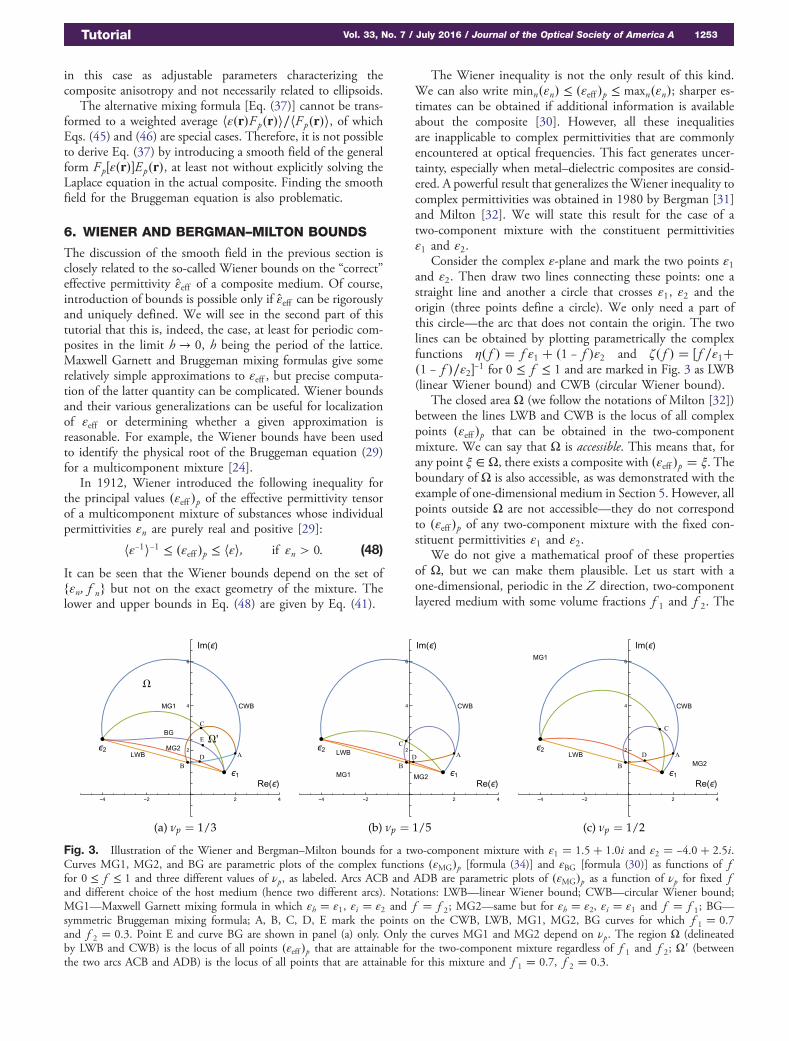
Fig. 3. Illustration of the Wiener and Bergman–Milton bounds for a two-component mixture with ε1 � 1.5� 1.0i and ε2 � −4.0� 2.5i.Curves MG1, MG2, and BG are parametric plots of the complex functions �εMG�p [formula (34)] and εBG [formula (30)] as functions of ffor 0 ≤ f ≤ 1 and three different values of νp, as labeled. Arcs ACB and ADB are parametric plots of �εMG�p as a function of νp for fixed fand different choice of the host medium (hence two different arcs). Notations: LWB—linear Wiener bound; CWB—circular Wiener bound;MG1—Maxwell Garnett mixing formula in which εh � ε1, εi � ε2 and f � f 2; MG2—same but for εh � ε2, εi � ε1 and f � f 1; BG—symmetric Bruggeman mixing formula; A, B, C, D, E mark the points on the CWB, LWB, MG1, MG2, BG curves for which f 1 � 0.7and f 2 � 0.3. Point E and curve BG are shown in panel (a) only. Only the curves MG1 and MG2 depend on νp. The region Ω (delineatedby LWB and CWB) is the locus of all points �εeff �p that are attainable for the two-component mixture regardless of f 1 and f 2; Ω 0 (betweenthe two arcs ACB and ADB) is the locus of all points that are attainable for this mixture and f 1 � 0.7, f 2 � 0.3.


principal value �εeff �z for this geometry will correspond to apoint A on the line CWB, and the principal values �εeff �x ��εeff �y will correspond to a point B on LWB. The points A andB are shown in Fig. 3 for f 1 � 0.7 and f 2 � 0.3. We will thencontinuously deform the composite while keeping the volumefractions fixed until we end up with a medium that is identicalto the original one except that it is rotated by 90° in the XZplane. In the end state, �εeff �x will correspond to point A and�εeff �y � �εeff �z will correspond to Point B. The intermediatestates of this transformation will generate two continuous tra-jectories [the loci of the points �εeff �x and �εeff �z] that connectA and B and one closed loop starting and terminating at B [theloci of the points �εeff �y]. Two such curves that connect A andB (the arcs ACB and ADB) are also shown in Fig. 3.

Now, let us scan f 1 and f 2 from f 1 � 1; f 2 � 0 tof 1 � 0; f 2 � 1. The points A and B will slide on the linesCWB and LWB from ε1 to ε2, and the curves that connectthem will fill the region Ω completely while none of thesecurves will cross the boundary of Ω. On the other hand,while deforming the composite between the states A and B,we can arrive at a state of an arbitrary three-dimensionalgeometry modulo the given volume fractions. Thus, for a two-component medium with arbitrary volume fractions, we canstate that (i) �εeff �p ∈ Ω and (ii) if ζ ∈ Ω, then there existsa composite with �εeff �p � ζ.

We now discuss the various curves shown in Fig. 3 in moredetail.

The curves marked as MG1, MG2 display the results com-puted by the Maxwell Garnett mixing formula (34) with vari-ous values of νp, as labeled. MG1 is obtained by assuming thatεh � ε1, εi � ε2, f � f 2. We then take the expression (34)and plot �εMG�p parametrically as a function of f for 0 ≤ f ≤1 for three different values of νp. MG2 is obtained in a similarfashion but using εh � ε2, εi � ε1, f � f 1.

Notice that, at each of the three values of νp used, the curvesMG1 and MG2 do not coincide because Eq. (34) is not “sym-metric” in the sense of Eq. (28). For this reason, MG1 andMG2 cannot be accurate simultaneously anywhere except in theclose vicinities of ε1 and ε2. Since there is no reason to preferMG1 over MG2 or vice versa (unless f 1 or f 2 are small), MG1andMG2 cannot be accurate in general, that is for any compositethat is somehow compatible with the parameters of the mixingformula. This point should be clear already from the fact thatcomposites that are not made of ellipsoids are not characterizablemathematically by just three depolarization factors νp.

However, in the limits νp → 0 and νp → 1, MG1 and MG2coincide with each other and with either LWB or CWB. Inthese limits, MG1 and MG2 are exact.

In panel (a), we also plot the curve BG computed accordingto Bruggeman mixing formula [Eq. (30)] with the “�” sign.This BG curve follows closely MG1 in the vicinity of ε1and MG2 in the vicinity of ε2. This result is expected sincethe Maxwell Garnett and Bruggeman approximations coincideto first order in f : see Eq. (31) and recall that f � f 2 for MG1and f � f 1 for MG2.

The two arcs ACB and ADB that connect the points A andB are defined by the following conditions: If continued to fullcircles, ACB will cross ε1 and ADB will cross ε2. The arcs can

also be obtained by plotting �εMG�p as given by Eq. (34) para-metrically as a function of νp for fixed f 1 and f 2. To plot thearc ACB, we set εh � ε1, εi � ε2 and f � f 2 in Eq. (34), justas was done in order to compute the curve MG1. However,instead of fixing νp and varying f , we now fix f � 0.3 andvary νp from 0 to 1. Similarly, the arc ADB is obtained bysetting εh � ε2, εi � ε1, f � f 1 and varying νp in the sameinterval.

The region delineated by the arcs ACB and ADB is denotedby Ω 0. It is important for the following reason. Above, we havedefined the region Ω, which is the locus of all points �εeff �p forthe two-component mixture regardless of the volume fractions.If we fix the latter to f 1 and f 2, the region of allowed �εeff �pcan be further narrowed. It is shown in [31,32] that this regionis precisely Ω 0. Note that the Maxwell Garnett approximation(34) with the same f 1 and f 2 yields the results on the boundaryofΩ 0. Conversely, any point on the boundary ofΩ 0 correspondsto Eq. (34) with some νp. The isotropic Bruggeman’s solution issafely inside Ω 0 [see point E in panel (a)].

Just like Ω, the region Ω 0 is also accessible. This means thateach point inside Ω 0 corresponds to a certain composite withgiven ε1, ε2, f 1, and f 2. However, it is not obvious how theboundaries of Ω 0 can be accessed. Above, we have seen that theboundaries of Ω are accessed by the solutions to the homog-enization problem in a very simple one-dimensional geometrywherein the smooth field S can be easily (and precisely) de-fined. The same is true for Ω 0. It can be shown [31] that thegeometry for which the boundary of Ω 0 is accessed is anassembly of coated ellipsoids that are closely packed to fillthe entire space. This is possible if we take an infinite sequenceof such ellipsoids of ever decreasing size. Note that all majoraxes of the ellipsoids should be parallel, the core and the shellof each ellipsoid should be confocal, and the volume fractionsof the ε1 and ε2 substances comprising each ellipsoid should befixed to f 1 and f 2. The arrangement in which ε1 is the coreand is the shell will give one circular boundary of Ω 0, and thearrangement in which ε2 is in the core and ε1 is in the shell willgive another boundary.

Of course, the above arrangement is a purely mathematicalconstruct. It is not realizable in practice. However, it is interest-ing to note that the Maxwell Garnett mixing formula [Eq. (34)]turns out to be exact in this strange geometry. In the special casewhen the ellipsoids are spheres, the isotropic Maxwell Garnettformula [Eq. (18)] is exact. This isotropic, arbitrarily densepackaging of coated spheres of progressively reduced radiiwas considered by Hashin and Shtrikman in 1962 [30].

We can now see why the anisotropic Maxwell Garnett mix-ing formula [Eq. (34)] is special. First, it samples the region Ωcompletely. In other words, any two-component mixture withε1- and ε2-type constituents has the effective permittivity prin-cipal values �εeff �p that are equal to a value �εMG�p produced byEq. (34) with the same ε1 and ε2 (but perhaps with differentvolume fractions). Second, Eq. (34) is restricted to Ω. In otherwords, any value �εMG�p produced by Eq. (34) is equal to�εeff �p of some composite with the same ε1 and ε2 (but perhapswith different volume fractions).

To conclude the discussion of bounds, we note that [31,32]contain an even stronger result. If, in addition to ε1; ε2; f 1; f 2,


it is also known that the composite is isotropic on average, thenthe allowed region for εeff (now a scalar) is further reduced toΩ 0 0 ⊂ Ω 0 ⊂ Ω. Here Ω 0 0 is delineated by yet another pair ofcircular arcs that connect the points C and D and, if continuedto circles, also cross the points A and B. These arcs are notshown in Fig. 3.

7. SCALING LAWS

Maxwell Garnett and Bruggeman theories give some approxi-mations to the effective permittivity of a composite ε̂eff . Wienerand Bergman–Milton bounds discussed in the previous sectiondo not provide approximations or define ε̂eff precisely butrather restrict it to a certain region in the complex plane.However, the very possibility of deriving approximations orplacing bounds on ε̂eff relies on the availability of an unambigu-ous definition of this quantity. We will sketch an approach todefining and computing ε̂eff in the second part of this tutorial.Now we note that this definition is expected to satisfy thefollowing two scaling laws [10].

The first law is invariance under coordinate rescalingr → βr, where β > 0 is an arbitrary real constant. In otherwords, the result should not depend on the physical size of theheterogeneities. Of course, one cannot expect a given theoryto be valid when the heterogeneity size is larger than thewavelength. Therefore, the above statement is not about thephysical applicability of a given theory. Rather, it is aboutthe mathematical properties of the theory itself. We can saythat any standard theory is obtained in the limit h → 0, whereh is the characteristic size of the heterogeneity, say, the latticeperiod. The result of taking this limit is, obviously, independentof h.

The second law is the law of unaltered ratios: If every εn of acomposite medium is scaled as εn → βεn, then the effective per-mittivity (as computed by this theory) should scale similarly,viz., ε̂eff → βε̂eff .

Theories (either exact or approximate) that satisfy the abovetwo laws can be referred to as standard. It is easy to see that theMaxwell Garnet and the Bruggeman theories are standard. Onthe other hand, the so-called extended homogenization theoriesthat consider magnetic and higher-order multipole moments ofthe inclusions do not generally satisfy the scaling laws.

8. SUMMARY AND OUTLOOK

In Sections 2–4, we have covered the material that one encoun-ters in standard textbooks. Sections 5–7 contain somewhat lessstandard, but still mathematically simple, material. The tutorialcould end here. However, we cannot help noticing that thearguments we have presented are not complete and not alwaysmathematically rigorous. There are several topics that we needto discuss if we want to gain a deeper understanding of thehomogenization theories in general and of the MaxwellGarnett mixing formula in particular.

First, the standard expositions of the Maxwell Garnett mix-ing formula and of the Lorentz molecular theory of polarizationrely heavily on the assumption that polarization field P�r� ��ε�r� − 1�∕4π�E�r� is the dipole moment per unit volume.But this interpretation is neither necessary for defining the con-stitutive parameters of the macroscopic Maxwell’s equations

nor, generally, correct. The physical picture based on thepolarization being the density of dipole moment is in manycases adequate, but in some other cases it can fail. We havebeen careful to operate only with total dipole moments of mac-roscopic objects. Still, this point requires some additional dis-cussion.

Second, the Lorentz local field correction relies on integrat-ing the electric field of a dipole over spheres or ellipsoids offinite radius. It can be assumed naively that, since the integralis convergent for some finite integration regions, it also con-verges over the whole space. But this assumption is mathemati-cally incorrect. The integral of the electric field of a static dipoletaken over the whole space does not converge to any result.Therefore, if we arbitrarily deform the surface that boundsthe integration domain, we would obtain an arbitrary integra-tion result. In fact, we have already seen that this resultdepends on whether the surface is spherical or ellipsoidal. Thisdependence, in turn, affects the Lorentz local field correction.Consequently, developing a more rigorous mathematicalformalism that does not depend on evaluation of divergentintegrals is desirable.

Third, we have worked mostly within statics. We did discussfinite frequencies in the sections devoted to smooth field andWiener and Bergman–Milton bounds, but not in any substan-tial detail. However, the theory of homogenization is almostalways applied at high frequencies. In this case, Eq. (2) is notapplicable; a more general formula must be used. Incidentally,the integral of the field of an oscillating dipole diverges evenmore strongly than that of a static dipole. It is also not correctto use the purely static expression for the polarizabilities atfinite frequencies.

The above topics will be addressed in the second part of thistutorial.

Funding. Agence Nationale de la Recherche (ANR) (ANR-11-IDEX-0001-02).

Acknowledgment. This work has been carried outthanks to the support of the A*MIDEX project (No. ANR-11-IDEX-0001-02) funded by the “Investissements d’Avenir”French government program, managed by the French NationalResearch Agency (ANR).

REFERENCES AND NOTES

1. J. C. M. Garnett, “Colours in metal glasses and in metallic films,”Philos. Trans. R. Soc. London A 203, 385–420 (1904).

2. J. C. M. Garnett, “Colours in metal glasses, in metallic films, and inmetallic solutions II,” Philos. Trans. R. Soc. London 205, 237–288(1906).

3. R. Resta, “Macroscopic polarization in crystalline dielectrics: thegeometrical phase approach,” Rev. Mod. Phys. 66, 899–915 (1994).

4. R. Resta and D. Vanderbilt, “Theory of polarization: a modernapproach,” in Physics of Ferroelectrics: A Modern Perspective(Springer, 2007), pp. 31–68.

5. D. M. Wood and N. W. Ashcroft, “Effective medium theory of opticalproperties of small particle composites,” Philos. Mag. 35(2), 269–280(1977).

6. G. A. Niklasson, C. G. Granqvist, and O. Hunderi, “Effective mediummodels for the optical properties of inhomogeneous materials,” Appl.Opt. 20, 26–30 (1981).


7. T. G. Mackay, A. Lakhtakia, and W. S. Weiglhofer, “Strong-property-fluctuation theory for homogenization of bianisotropic composites:formulation,” Phys. Rev. E 62, 6052–6064 (2000).

8. W. T. Doyle, “Optical properties of a suspension of metal spheres,”Phys. Rev. B 39, 9852–9858 (1989).

9. R. Ruppin, “Evaluation of extended Maxwell–Garnett theories,” Opt.Commun. 182, 273–279 (2000).

10. C. F. Bohren, “Do extended effective-medium formulas scale prop-erly?” J. Nanophoton. 3, 039501 (2009).

11. In a spherical system of coordinates �r; θ;φ�, the angular average ofcos2 θ is 1∕3; that is, hcos2i � �4π�−1 R 2π

0 dφRπ0 sin θdθ cos2 θ � 1∕3.

12. Equation (8) can be obtained by using the expression ϕ�r� �R �ρ�R�∕jr − Rj�d3R for the electrostatic potential ϕ�r�, assuming thatthe charge density ρ�R� is localized around a point r 0, using the ex-pansion 1∕jr − Rj � 1∕jr − r 0j � �R − r 0� · ∇r 0 �1∕jr − r 0j� �…, definingthe dipole moment of the system as d � R

rρ�r�d3r, and, finally, com-puting the electric field according to E�r� � −∇rϕ�r�.

13. E. M. Purcell and C. R. Pennypacker, “Scattering and absorption of lightby nonspherical dielectric grains,” Astrophys. J. 186, 705–714 (1973).

14. B. T. Draine, “The discrete-dipole approximation and its application tointerstellar graphite grains,” Astrophys. J. 333, 848–872 (1988).

15. B. T. Draine and J. Goodman, “Beyond Clausius–Mossotti: wavepropagation on a polarizable point lattice and the discrete dipoleapproximation,” Astrophys. J. 405, 685–697 (1993).

16. L. L. Foldy, “The multiple scattering of waves. I. General theory of iso-tropic scattering by randomly distributed scatterers,” Phys. Rev. 67,107–119 (1945).

17. M. Lax, “Multiple scattering of waves,” Rev. Mod. Phys. 23, 287–310(1951).

18. P. B. Allen, “Dipole interactions and electrical polarity in nanosystems:the Clausius-Mossotti and related models,” J. Chem. Phys. 120,2951–2962 (2004).

19. D. Vanzo, B. J. Topham, and Z. G. Soos, “Dipole-field sums, Lorentzfactors and dielectric properties of organic molecular films modeledas crystalline arrays of polarizable points,” Adv. Funct. Mater. 25,2004–2012 (2015).

20. Of course, infinite media do not exist in nature. Here we mean a hostmedium that is so large that the field created by the dipole is negligibleat its boundaries. In general, one should be very careful not to make a

mathematical mistake when applying the concept of “infinite medium,”especially when wave propagation is involved.

21. D. A. G. Bruggeman, “Berechnung verschiedener physikalischerKonstanten von heterogenen Substanzen. I. Dielektrizitätskonstantenund Leitfähigkeiten der Mischkörper aus isotropen Substanzen,” Ann.Phys. 416, 665–679 (1935).

22. D. A. G. Bruggeman, “Berechnung verschiedener physikalischerKonstanten von heterogenen Substanzen. II. Dielektrizitätskonstantenund Leitfähigkeiten von Vielrkistallen der nichtregularen Systeme,”Ann. Phys. 417, 645–672 (1936).

23. S. Berthier and J. Lafait, “Effective medium theory: mathematicaldetermination of the physical solution for the dielectric constant,”Opt. Commun. 33, 303–306 (1980).

24. R. Jansson and H. Arwin, “Selection of the physically correct solutionin the n-media Bruggeman effective medium approximation,” Opt.Commun. 106, 133–138 (1994).

25. C. F. Bohren and D. R. Huffman, Absorption and Scattering of Lightby Small Particles (Wiley, 1998).

26. D. Schmidt and M. Schubert, “Anisotropic Bruggeman effectivemedium approaches for slanted columnar thin films,” J. Appl. Phys.114, 083510 (2013).

27. S. M. Rytov, “Electromagnetic properties of a finely stratified medium,”J. Exp. Theor. Phys. 2, 466–475 (1956).

28. This is true for sufficiently small h, as long as the phase shift of thewave propagating in the structure over one period is small comparedto π. Homogenization is possible only if this condition holds.

29. O. Wiener, “Die Theorie des Mischkörpers für das Feld derStationären Strömung. Erste Abhandlung: Die Mittelwertsätze fürKraft, Polarisation und Energie,” Abhandlungen der Mathathematisch-Physikalischen Klasse der Königl. Sächsischen Gesellschaft derWissenschaften 32, 507–604 (1912).

30. Z. Hashin and S. Shtrikman, “A variational approach to the theory ofthe effective magnetic permeability of multiphase materials,” J. Appl.Phys. 33, 3125–3131 (1962).

31. D. J. Bergman, “Exactly solvable microscopic geometries and rigor-ous bounds for the complex dielectric constant of a two-componentcomposite material,” Phys. Rev. Lett. 44, 1285–1287 (1980).

32. G. W. Milton, “Bounds on the complex dielectric constant of acomposite material,” Appl. Phys. Lett. 37, 300–302 (1980).


Documents

Introduction to the Maxwell Garnett approximation: tutorial · Introduction to the Maxwell Garnett approximation: tutorial ... This tutorial is devoted to the Maxwell Garnett