Introduction to the Dynamic Universe - Elisasuntola/DU_library/2007_Introduction_to_DU.pdf · The Dynamic Universe approach is just a detailed analysis of combining Feyn- man’s

Introduction to the Dynamic Universe

Tuomo Suntola

2008

2 The Dynamic Universe

Abstract

The Dynamic Universe is a holistic model of physical reality starting from whole space as a spherically closed zero-energy system. Instead of extrapolating the cosmo-logical appearance of space from locally defined field equations, locally observed phenomena are derived from the conservation of the zero-energy balance of motion and gravitation in whole space. The energy structure of space is described in terms of nested energy frames starting from hypothetical homogeneous space as the universal reference and proceeding down to local frames in space. Time is decoupled from space – the fourth dimension has a geometrical meaning as the radius of the sphere closing the three-dimensional space. Relativity in the Dynamic Universe is the meas-ure of the locally available share of total energy – clocks in fast motion or in a strong gravitational field do not lose time because of slower flow of time but because more energy is bound into interactions in space. For local observations, the DU predictions are essentially the same as the corresponding predictions derived from the theory of relativity. At the extremes, at cosmological distances and in the vicinity of local singu-larities in space however, differences become remarkable – e.g. galactic space in the DU appears in Euclidean geometry, and the magnitudes of high redshift supernovae are explained without assumptions of dark energy or accelerating expansion. Black holes in DU space have stable orbits down to the critical radius. Instead of a sudden Big Bang, the energy buildup in Dynamic Universe is seen as a continuous process from infinity in the past to infinity in the future.

PACS codes: 04.20.Cv, 95.36.+x, 95.10.-a, 98.65.-r

The Dynamic Universe 3

Contents

1.1 Motion and gravitation in homogeneous space 9 1.1.1 Postulates and definitions 9 1.1.2 Zero-energy balance in hypothetical homogeneous space 10 1.1.3 The primary energy buildup 11

1.2 Interactions in space 15 1.2.1 Global and local frames 15 1.2.2 Unified expression of energy 16 1.2.3 The energy vector 17

1.3 Symmetries in zero-energy space 18 1.3.1 The zero-energy balance of motion and gravitation 18 1.3.2 Conservation of energy in mass center buildup 20 1.3.3 Kinetic energy and inertial work 21 1.3.4 Motion as central motion in spherical space 25 1.3.5 Motion in parent frame 26 1.3.6 Emission of radiation quanta 27

1.4 The system of nested energy frames 28 1.4.1 The linkage of local and global 28 1.4.2 Earth gravitational frame 30

2.1 Electromagnetic energy 33 2.1.1 The Coulomb energy 33 2.1.2 The quantum of radiation 33 2.1.3 Mass wave 36

2.2 Electromagnetic objects 37 2.2.1 Hydrogen-like atoms 37 2.2.2 Electromagnetic resonator as an energy object 39

3.1 Celestial mechanics in local gravitational frame 42 3.1.1 Cylinder coordinate system 42 3.1.2 Orbital velocity and the velocity of free fall 45

Abstract 2

Contents 3

Introduction 5

1. Spherically closed space 9

2. Electromagnetic energy and a quantum of radiation 33

3. Properties of local space 42


3.1.3 Orbital period in the vicinity of local singularity 46 3.1.4 Perihelion advance 47 3.1.5 Sub-frame in a gravitational frame 48 3.1.6 The frequency of atomic oscillators 48

3.2 Propagation of light 49 3.2.1 Shapiro delay 49 3.2.2 Bending of light path near a mass center 52 3.2.3 Gravitational shift of electromagnetic radiation 53 3.2.4 Doppler effect and transmission time 54 3.2.5 Sagnac effect 56

4. Cosmological appearance of DU space 59

4.1 Distances and the observed angular size 59 4.1.1 Cosmological principle in spherically closed space 59 4.1.2 Optical distance and the Hubble law 59 4.1.3 Angular sizes of a standard rod and expanding objects 62

4.2 Observation of radiation 65 4.2.1 Apparent magnitude of standard candle 65 4.2.2 Surface brightness of expanding objects 68 4.2.3 Microwave background radiation 68

5. Summary 69

Acknowledgements 71

References 72


Introduction

Newtonian physics is local by its nature. There are no overall limits to space or to physical quantities. Newtonian space is Euclidean until infinity, and velocities in space grow linearly as long as there is constant force acting on an object.

The theory of relativity introduces finiteness as finiteness of velocities by defining the coordinate quantities, time and distance, as functions of velocity and gravitational state so that the velocity of light appears as an invariant and the maximum velocity obtainable in space. In the framework of relativity theory, clocks in a high gravitation-al field and in fast motion conserve the local proper time but lose coordinate time re-lated to time measured by a clock at rest in a zero gravitational field.

In the Dynamic Universe, finiteness comes from the finiteness of total energy in space — finiteness of velocities in space is a consequence of the zero-energy balance, which does not allow velocities higher than the velocity of space in the fourth dimen-sion. The velocity of space in the fourth dimension is determined by the zero-energy balance of motion and gravitation of whole space and it serves as the reference for all velocities in space.

The total energy is conserved in all interactions in space. Motion and gravitation in space reduce the energy available for internal processes within an object. Atomic clocks in fast motion or in high gravitational field in DU space do not lose time be-cause of slower flow of time but because they use part of their total energy for kinetic energy and local gravitation in space.

In his lectures on gravitation in early 1960’s Richard Feynman [1] stated: “If now we compare this number (total gravitational energy M

2G/R) to the total rest energy of the universe, Mc

2, lo and behold, we get the amazing result that GM

2/R = M c2, so that the total energy of the universe is zero. — It is exciting to

think that it costs nothing to create a new particle, since we can create it at the center of the universe where it will have a negative gravitational energy equal to Mc

2. — Why this should be so is one of the great mysteries—and therefore one of the impor-tant questions of physics. After all, what would be the use of studying physics if the mysteries were not the most important things to investigate”.

and further [2] “...One intriguing suggestion is that the universe has a structure analogous to that

of a spherical surface. If we move in any direction on such a surface, we never meet a


boundary or end, yet the surface is bounded and finite. It might be that our three-dimensional space is such a thing, a tridimensional surface of a four sphere. The ar-rangement and distribution of galaxies in the world that we see would then be some-thing analogous to a distribution of spots on a spherical ball.”

Once we adopt the idea of the fourth dimension with metric nature, Feynman’s

findings open up the possibility of a dynamic balance of space: the rest energy of mat-ter is the energy of motion mass in space possesses due to the motion of space in the direction of the radius of the 4-sphere. Such a motion is driven by the shrinkage force resulting from the gravitation of mass in the structure. Like in a spherical pendulum in the fourth dimension, contraction building up the motion towards the center is fol-lowed by expansion releasing the energy of motion gained in the contraction.

The Dynamic Universe approach is just a detailed analysis of combining Feyn-man’s “great mystery” of zero-energy space to the “intriguing suggestion of spherical-ly closed space” by the dynamics of a four sphere.

By equating the integrated gravitational energy in the spherical structure with the energy of motion created by momentum in the direction of the 4-radius we enter into zero-energy space with motion and gravitation in balance. It may not be a surprise that by assuming the presently relevant estimates of the mass density and Hubble radius of space, we can calculate the velocity of spherically closed space in the direction of the 4-radius as 300,000 km/s, equal to the velocity of light in space.

In fact, space as the surface of a four sphere is based on quite an old and original idea of describing space as a closed but endless entity. Spherically closed space was outlined in the 1900th century by Ludwig Schläfli, George Riemann and Ernst Mach. Space as the 3-dimensional surface of a four sphere was also Einstein’s original view of the cosmological picture of general relativity he suggested in 1917 [3]. The prob-lem, however, was that Einstein was looking for a static solution — it was just to pre-vent the dynamics of spherically closed space that made Einstein to add the cosmolog-ical constant to the theory. We also find out that dynamic space requires metric fourth dimension which does not fit to the concept of four-dimensional spacetime the theory of relativity is built on.

In Dynamic Universe time and distance, the basic coordinate quantities and the key attributes for human conception, are absolute and universal. The fourth dimension is metric by its nature although inaccessible from three-dimensional space.

In a local frame, a rough translation from relativity theory to the Dynamic Universe is given by a physical interpretation of the energy four-vector as the vector sum of momentum p4 = mc4 in a physical fourth dimension and momentum p in a space direc-tion.

22 2 2totE c mc p (a)


Relativity in Dynamic Universe is a direct consequence of the conservation of the total energy in interactions in space. It does not rely on the relativity principle, space-time, the equivalence principle, Lorentz covariance, or the invariance of the velocity of light — but just on the zero-energy balance of space.

In a detailed analysis, the locally available rest energy mass object m possesses in the n:th energy frame is

2 20 0 0 0

1

1 1n

rest i ii

E c c mc m c

p (b)

where c0 is the velocity of light in hypothetical homogeneous space, which is equal to the velocity of space in the direction of the 4-radius R4. The factors i = GMi/c

2 and i = vi/ci are the gravitational factor and the velocity factor relevant to the local frame, respectively. On the Earth, for example, the gravitational factors define the gravita-tional state of an object on the Earth, the gravitational state of the Earth in the solar frame, the gravitational state of the solar frame in the Milky Way frame, etc. The ve-locity factors related to an object on Earth comprise the rotational velocity of the Earth and the orbital velocities of each sub-frame in each one’s parent frame.

The concept of motion in Dynamic Universe is twofold; velocity as the measure of

kinetic energy is related to the state of rest in the energy frame where the velocity is obtained — the observed relative velocity between two objects serves as the measure of the change in the distance between the objects, which does not define the content of kinetic energy each object is carrying.

Most important, spacetime symmetries of the special and general theory of relativi-ty are replaced by symmetries resulting from the zero-energy balance of energies.

Equation (b) means that the locally available rest energy is a function of the gravi-tational state, and the velocity of the object studied. Substituting (b) for the rest energy of electron in Balmer’s equation the characteristic frequency related to an energy tran-sition obtains the form

2 20 1

1

1 1 1 1n

local i i n n ni

f f f

(c)

where frequency fn–1 is the characteristic frequency of the atom at rest far from the local mass center in the local frame. The last form of equation (c) is essentially equal to the expression of coordinate time frequency in Earth, or Earth satellite clocks in the GR framework. The physical message of (c) is that “the greater the share of total energy which used for motions and gravitational interactions in space the less energy is left for running internal processes”.


The Dynamic Universe links the energy of any localized object to the energy of whole space. Relativity in Dynamic Universe means relativity of local to whole.

The balance of the rest energy and the global gravitational energy means also that antimatter of any localized mass object in space is the mass of the rest of space

0rest globalE E (d)

At the cosmological scale an important consequence of the linkage between local space and whole space is that local gravitational systems grow in direct proportion to the expansion of space thus, together with the spherical symmetry, explaining the ob-served Euclidean appearance and surface brightnesses of galaxies in space. The mag-nitude redshift relation of a standard candle in the DU framework is in an accurate agreement with observations without assumptions of dark energy or any other free parameters. Moreover, the zero-energy balance in the DU leads to stable orbits down to the critical radius in the vicinity of local singularities in space.

In the DU framework the energy of a quantum of radiation appears as the unit energy carried by a cycle of radiation

00 0 0

hE c c c m c c

p (e)

where h0 hc is referred to as the intrinsic Planck constant which is solved from Maxwell’s equation, by observing that a point emitter in DU space which is moving at velocity c in the fourth dimension can be regarded as one-wavelength dipole in the fourth dimension. Such a solution shows also that the fine structure constant is a purely numerical or geometrical factor without linkage to any physical constant.

The quantity h0/ m [kg] in (e) is referred to as the mass equivalence of radia-tion. Equally, Coulomb energy is expressed in form

20 0

0 0 02 2C C

e hE c c c c c m c

r r

(f)

where is the fine structure constant and the quantity h0/2 r mC is the mass equiva-lence of Coulomb energy.

Equations (b), (e), and (f) give a unified expression of energies which is essential in a detailed energy inventory in the course of the expansion of space and in interactions within space. The zero-energy concept in the Dynamic Universe follows bookkeeper’s logic — the accounts for the energy of motion and potential energy are kept in balance throughout the expansion and within any local frame in space.

Historically, the basis of the zero-energy concept was first time expressed by Gottfried Leibniz, the great philosopher, mathematician, and physicist contemporary with Isaac Newton. Leibniz introduced the zero-energy principle by stating that vis


viva, the living force mv2 (kinetic energy) is obtained against release of vis mortua, the dead force (potential energy) [4]. Inherently, such an approach defines the state of rest as a property of an energy system where kinetic energy (vis viva) is created.

It also looks like Leibniz’s monads as “perpetual, living mirrors of the universe”, reflected the idea of wholeness and the complementary nature of local and global in material objects in Dynamic Universe. There is no need to expect antimatter in space; via the zero-energy balance of motion and gravitation, the rest energy of any localized mass object is counterbalanced by the gravitational energy due to all rest of mass in space.

The Dynamic Universe is a holistic description of physical reality [5]. The system of nested energy frames in spherically closed space links local structures and pheno-mena to space as whole. The zero-energy approach in the DU allows the derivation of local and cosmological predictions with a minimum of postulates and by honoring universal time and distance as the basic coordinate quantities for human conception. In a mathematically clear and straightforward way it produces precise predictions for phenomena in relativistic physics, celestial mechanics, and cosmology, and allows a unified expression of energies showing the linkage between electromagnetic quantities and mass objects.

The Dynamic Universe means major rethinking of the cosmological structure and development of the universe. Instead of a sudden Big Bang switching on time, energy, and the laws of nature, the buildup and release of energy in Dynamic Universe devel-ops in a contraction and expansion process from emptiness in infinity in the past through singularity to emptiness in infinity in the future.

1. Spherically closed space

1.1 Motion and gravitation in homogeneous space

1.1.1 Postulates and definitions

The Dynamic Universe model assumes that space is spherically closed through the fourth dimension; i.e. space is described as the 3-dimensional surface of a 4-dimensional sphere free to contract and expand maintaining a zero-energy balance of motion and gravitation in the system. Mass as the substance for the expression of energy is the primary conservable in space.

For calculating the zero-energy balance in spherically closed space the inherent forms of the energies of gravitation and motion are defined as follows:


1) The inherent gravitational energy is defined in homogeneous 3-dimensional space

as Newtonian gravitational energy

0gV

dV rE mG

r (1.1.1:1)

where G is the gravitational constant, is the density of mass, and r is the dis-tance between m and dV. Total mass in homogeneous space is

V

M dV V (1.1.1:2)

In spherically closed homogeneous 3-dimensional space the total mass is 2 3

02M R , where R0 is the radius of space in the fourth dimension.

2) The inherent energy of motion is defined in environment at rest as the product of the velocity and momentum

2

0mE v v m mv p v (1.1.1:3)

The last form of the energy of motion in (1.1.1:3) has the form of the first formulation of kinetic energy, vis viva, “the living force” suggested by Gottfried Leibniz in late 1600’s [4].

1.1.2 Zero-energy balance in hypothetical homogeneous space

The energy of motion mass m at rest in space possesses due to the motion of space in the fourth dimension is referred to as the rest energy of matter. In hypothetical ho-mogeneous space, the rest energy is

0 0 0 0restE c c mc p (1.1.2:1)

where p0 is the momentum of mass m and c0 is the velocity of space in the direction of the 4-radius. The symbol c is used for the velocity of space because it is shown that the velocity of space in the fourth dimension defines the maximum velocity and the velocity of light in space.

The energy of gravitation resulting from total mass M on mass m is referred to as global gravitational energy. In spherically closed homogeneous space the global gra-vitational energy is

0

"global

V

dV GM mE mG

r R (1.1.2:2)


where M" = 0.776 M is the mass equivalence at the center of “hollow“ spherically closed space with radius R0. Obviously, any mass m in homogeneous space is at dis-tance R0 from mass M".

For mass m at rest in hypothetical homogeneous space with 4-radius R0 the balance of the energies of motion and gravitation is

20

0

"0rest global

GM mE E mc

R (1.1.2:3)

The rest energy is a local expression of energy of an object. In spherically closed space the rest energy of an object is balanced by the global gravitational energy result-ing from all the rest of mass in space.

The complementarity of energies — the rest energy and the global gravitational energy — means also complementarity of local and global.

For total mass M the balance of the energies of motion and gravitation in hypo-thetical homogeneous space is

20

0

"0rest tot global tot

GME E M c M

R (1.1.2:4)

Force in Dynamic Universe is the manifestation of a natural trend towards mini-mum potential energy. Force is expressed as the negative of the gradient of potential energy or in terms of a change of momentum.

1.1.3 The primary energy buildup

Solved from (1.1.2:4), velocity c0 that maintains the zero-energy balance of motion and gravitation in spherically closed space is

2 30

0 00 0

0.776 2"1.246

G RGMc R G

R R

(1.1.3:1)

where is the average mass density in space. Spherically closed space is accelerated by its own gravitation in a contraction phase

from infinite 4-radius to singularity creating the energy of motion against a release of gravitational energy. In the expansion phase after passing the singularity the energy of motion gained in the contraction is paid back to gravitational energy. In the contrac-tion space releases volume and obtains velocity, in the expansion phase velocity is released to recover the volume. In energy bookkeeping, the rest energy of matter, the energy mass possesses due to the motion of space in the fourth dimension is balanced by an equal energy debt to global gravitation (Fig 1.1.3-1).


Figure 1.1.3-1. Energy buildup and release in spherical space. In the contraction phase, the velocity

of motion increases due to the energy gained from loss of gravitation. In the expansion phase, the ve-locity of motion gradually decreases, while the energy of motion gained in contraction is returned to gravity.

The contraction and expansion of spherically closed space is the primary energy buildup process creating the rest energy of matter as the complementary counterpart to the global gravitational energy.

Based on observations of the Hubble constant, space in its present state is in the ex-pansion phase with radius R0 equal to about 14 billion light years. By applying R0 = 14 billion light years and by setting the mass density equal to = 5.010–27 [kg/m3], which is about half of the critical density 0 in the standard cosmology model, velocity c0 in (1.1.3:1) obtains the value c0 c = 300 000 [km/s].

20mE mc

0

"g

GME m

R

Energy of motion

Energy of gravitation

Expansion

time

Contraction


Figure 1.1.3-2. The decreasing expansion velocity of space in the direction of R0. Present deceleration

of the expansion velocity, and with it the velocity of light, is about 3.6 % per billion years. The velocity of light will drop to half of the present value in about 65 billion years and to 1 m/s in about 2 1026 billion years.

When solved as a function of time, the expansion velocity since singularity be-comes

1/ 31 34

0

2"

3

dRc GM t

dt

(1.1.3:2)

and the time since singularity becomes

4

944

4 4 00

1 2 2 19.3 10 l.y.

3 3

RR

t dRc c H

(1.1.3:3)

The velocity of expansion and, accordingly, the velocity of light decelerate in the course of expansion as

0 01

3

dc c

dt t (1.1.3:4)

The present deceleration rate of the velocity of light is dc0/c0 3.610–11 /year (Fig 1.1.3-2).

A detailed analysis shows that the maximum velocity achievable in space is equal to the velocity of space in the fourth dimension. In zero-energy space the rate of atom-ic processes, like the characteristic emission and absorption frequencies and radioac-tive decay occur in direct proportion to the velocity of the expansion and, accordingly, to the velocity of light in space. As a result, the velocity of light is observed as con-stant at any time during the expansion.

108 m/s

0

3

6

9

0 20 40 109 years 10 30


Figure 1.1.3-3. (a) Dimensions of galaxies and other gravitationally bound systems expand in direct

proportion to the expansion of space. (b) Localized objects bound by electromagnetic forces conserve their size. The characteristic wavelength emitted by atomic objects is conserved. (c) The wavelength of electromagnetic radiation propagating in space increases in direct proportion to the expansion of space. As a consequence the observed wavelength is redshifted.

In cosmological observables the faster rate of natural processes is seen, e.g., as a faster rate of radioactive decay in the past – correcting the age estimates of the un-iverse given by radiometric dating. It also means a faster rate of the development of galaxy structures in the early universe.

Conservation of the total gravitational energy in space links the radii of gravita-tionally bound local systems to the 4-radius of space — local systems expand in direct proportion to the expansion of space. As a consequence of the linkage distant space has Euclidean appearance in a full agreement with observations.

Atomic radii are not subject to expansion with the expansion of space, i.e. material objects conserve their dimensions. As shown by Balmer’s equations, the wavelength of characteristic emission is directly proportional to Bohr radius. Once the Bohr radius is conserved then also the emission wavelength is conserved. The wavelength of elec-tromagnetic radiation propagating in space increases in direct proportion to the expan-sion of space, which means that the observed characteristic wavelength from distant objects is redshifted relative to the reference wavelength of same transition at the time of observation, Fig. 1.1.3-3.

In the DU framework the basic form of matter is unstructured “dark matter” cha-racterized as radiation-like form of matter.

O

R0

(b)

R0

O

(a)

R0(1)

emitting object

O

R0(2)

t(2)

t(1)

(c)


1.2 Interactions in space

1.2.1 Global and local frames

The initial condition in space is considered as the state at rest with all mass un-iformly distributed within space. The state at rest in space means that any mass m in space has the momentum and velocity given by the expansion of the structure in the direction of the 4-radius. Hypothetical homogeneous space is used as the universal frame of reference for all interactions in space. Hypothetical homogeneous space has perfect spherical symmetry. The barycenter of mass in space is in the center of the four-dimensional sphere defining the three-dimensional space. Mass equivalence M" in the barycenter is a hypothetical mass that results in the same gravitational energy on any mass m in space as does the integrated gravitational energy of all mass in homo-geneous spherical space. Due to the expansion of space at velocity c0 in the direction of the 4-radius R0, masses m at rest at distance d = R0 from each other in spherical space have recession velocity

0recessionv c (1.2.1:1)

relative to each other. Since masses m are at rest in their location in space they have momentum only in the direction of the R0 radius, and the relative velocity between the masses is not associated with momentum of kinetic energy (Fig. 1.2.1-1).

Figure 1.2.1-1. (a) Hypothetical homogeneous space has the shape of the 3-dimensional “surface”

of a perfect 4-dimensional sphere. Mass is uniformly distributed in the structure and the barycenter of mass in space is in the center of the 4-sphere. Mass m is a test mass in hypothetical homogeneous space. (b) In a local presentation a selected space direction is shown as the Re0 axis, and the fourth dimension which in hypothetical homogeneous space is the direction of R0 is shown as the Im0 axis. The velocity of light in hypothetical homogeneous space is equal to the expansion velocity c0.

m

0 00mE c p

00

"g

GM mE

R

0mE

0gE

(a) (b)

"M

0Im

0Re

0mE 0gE

m

m

0Im

0Im0Re

0Re


1.2.2 Unified expression of energy

For a detailed analysis of the symmetries and the conservation of energy in local interactions in space it is necessary to express electromagnetic energy in a form dis-tinguishing the mass equivalence of electromagnetic energy and the velocity of light. The energy of electromagnetic radiation has the form of the energy of motion

rad radE c p (1.2.2:1)

where momentum prad has the direction of the propagation of the radiation in space; the momentum of electromagnetic energy has no component in the fourth dimension.

In DU space moving at c in the fourth dimension a point emitter can be regarded as one-wavelength dipole in the fourth dimension. Solved from Maxwell’s equation the energy of one cycle of radiation from such a dipole is [5,6]

2 3 2 2 2 00 0 0 01.1049 2

hPE N e c f N hf N c c c m c

f

(1.2.2:2)

where h0 h/c0 [kgm] is referred to as the intrinsic Planck constant. For a point source, factor 1.1049 related to the radiation geometry of the antenna in the fourth dimension (see Section 2.1.2). The quantity m [kg]

3 22 20 0 0

0

1.1049 2;

e h hm N N m

(1.2.2:3)

is defined the mass equivalence of radiation. In the DU framework, a quantum of electromagnetic radiation is the energy carried

by one cycle of radiation emitted by a single transition of a unit charge in a point source, i.e. N =1 in equation (1.2.2:2)

0

0 0 00 0rad

hE c c m c c c

p (1.2.2:4)

A unified expression of Coulomb energy is obtained by applying vacuum permea-bility 0 and the fine structure constant [which in the DU framework is a numerical constant independent of any physical constants, see equation (2.1.2:6)]

21 2 0 0c 0 0 0 c4 2

q q hE c c N c c c m c

r r

(1.2.2:5)

where

20 0

1 2 1 24 2c

e hm N N N N

r r

(1.2.2:6)


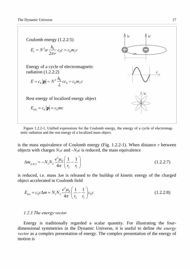
Figure 1.2.2-1. Unified expressions for the Coulomb energy, the energy of a cycle of electromag-

netic radiation and the rest energy of a localized mass object.

is the mass equivalence of Coulomb energy (Fig. 1.2.2-1). When distance r between objects with charges N1e and –N2e is reduced, the mass equivalence

20

1 22 1

1 1

4c r

em N N

r r

(1.2.2:7)

is reduced, i.e. mass m is released to the buildup of kinetic energy of the charged object accelerated in Coulomb field

20

0 1 2 02 1

1 1

4kin

eE c c m N N c c

r r

(1.2.2:8)

1.2.3 The energy vector

Energy is traditionally regarded a scalar quantity. For illustrating the four-dimensional symmetries in the Dynamic Universe, it is useful to define the energy vector as a complex presentation of energy. The complex presentation of the energy of motion is

ic ic

c

ic

Coulomb energy (1.2.2:5)

Energy of a cycle of electromagnetic radiation (1.2.2:2)

Rest energy of localized energy object

2 0c 0 0 c2

hE N c c c m c

r

2 00 0 0

hE c N cc c m c p

(0) 0 0E c c mc p


0 0 0 0* * ' " ' i " ' i "m m mE c E E c p c p c p p p (1.2.3:1)

where the imaginary part means the energy equivalence of momentum in the local fourth dimension. Real components of energies are marked with single apostrophe (') and the imaginary components with double apostrophe ("). Complex energies com-prising the real and imaginary components are marked with superscript (*).

The complex presentation of the energy of gravitation is

* ' "g g gE E E (1.2.3:2)

where E”g, the imaginary part, is the global gravitational energy resulting from all mass uniformly in spherically closed space.

The scalar value of the energy vector (1.2.3:1) is denoted as

*m mE E (1.2.3:3)

The kinetic energy of an object moving at velocity = v/c in a local frame is the to-tal energy of motion minus the energy of motion the object has at rest in the local frame

0 0 00kin m mE E E c c p p p (1.2.3:4)

Local gravitational energy is defined as the total energy of gravitation minus the global energy in the local frame. Generally, only the scalar value of local gravitational energy is of interest

* "g gg localE E E (1.2.3:5)

The energy vector of electromagnetic radiation is defined as the Poynting vector [W/m2] multiplied by the cycle time and the cross section area of radiation, which gives the total energy carried by a cycle of radiation. Electromagnetic radiation propa-gates in space directions; the energy vector of radiation has real component only.

1.3 Symmetries in zero-energy space

1.3.1 The zero-energy balance of motion and gravitation

Mass at rest in hypothetical homogeneous space has the energies of motion and gravitation in the imaginary direction only

20 4 0 0 0* i " ; "m m rest mE E E E c c mc mc p (1.3.1:1)


Figure 1.3.1-1. Rest energy and the global gravitational energy (a) in hypothetical homogeneous

space where c = c0 and R” = R0, and (b) in locally tilted space where c < c0 and the apparent distance to mass equivalence M” is increased as R”> R0.

where c0 is the velocity of space in the direction of 4-radius R0, and

0

"* i " ; "g g g

GM mE E E

R (1.3.1:2)

In locally tilted space the velocity of space in the direction of the local imaginary axis is reduced as

0 cosc c (1.3.1:3)

and the rest energy is expressed as

0restE c mc (1.3.1:4)

The global gravitational energy in tilted space is reduced as

0

" "" cos

" "g

GM m GM mE

R R

(1.3.1:5)

where R” is the apparent distance to the mass equivalence M" (Fig. 1.3.1-1). Quanti-ties c0 and R”0 in (1.3.1:3) and (1.3.1:5), respectively, refer to apparent homogene-ous space around locally tilted space [also the apparent homogeneous space may be tilted relative to hypothetical homogeneous space (see Section 1.4)].

m

0 0restE c mc

0

""g

GM mE

R

0Im

0Re m

0Im

0restE c mc

""

"g

GM mE

R

a b


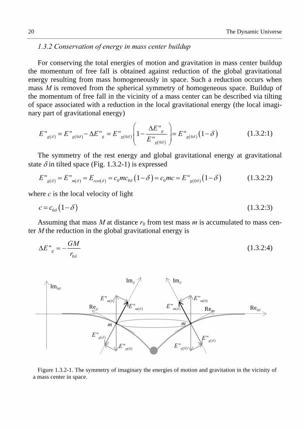
1.3.2 Conservation of energy in mass center buildup

For conserving the total energies of motion and gravitation in mass center buildup the momentum of free fall is obtained against reduction of the global gravitational energy resulting from mass homogeneously in space. Such a reduction occurs when mass M is removed from the spherical symmetry of homogeneous space. Buildup of the momentum of free fall in the vicinity of a mass center can be described via tilting of space associated with a reduction in the local gravitational energy (the local imagi-nary part of gravitational energy)

0 0 00

"" " " " 1 " 1

"g

gg g g gg

EE E E E E

E

(1.3.2:1)

The symmetry of the rest energy and global gravitational energy at gravitational state in tilted space (Fig. 1.3.2-1) is expressed

0 0 0 0" " 1 " 1g m rest gE E E c mc c mc E (1.3.2:2)

where c is the local velocity of light

0 1c c (1.3.2:3)

Assuming that mass M at distance r0 from test mass m is accumulated to mass cen-ter M the reduction in the global gravitational energy is

0

"g

GME

r

(1.3.2:4)

Figure 1.3.2-1. The symmetry of imaginary the energies of motion and gravitation in the vicinity of

a mass center in space.

"gE

0Re Re

0Im

Re "mE

"gE

"mE

mm

ImIm

0"mE 0"mE

0"gE 0"gE


and the gravitational factor becomes

0 0 0 0 0 0 0

";

"c

c

rMR GM GMr

M r r c c r c c

(1.3.2:5)

where rc is the critical radius corresponding to radius where space is tilted 90. (Obs. The critical radius in the Schwarzschild space is 2GM/c2, which is twice the critical radius rc in the DU.)

1.3.3 Kinetic energy and inertial work

The kinetic energy of an object moving at velocity = v/c in a local frame was de-fined as the total energy of motion minus the energy of motion the object has at rest in the local frame (1.2.3:4). The total energy of motion of an object in free fall from the state of rest far from the local mass center is, Fig. 1.3.3 (a)

0 0 0 0 0Re Im 0 Imtotalm totalE c c c c mc p p p p (1.3.3:1)

The rest energy of an object at gravitational state characterized by tilting angle is

0 0ImrestE c c mc p (1.3.3:2)

and the kinetic energy of free fall from the state of rest far from the local mass center is

0 0 0 0 0 0kin ff m total restE E E c mc c mc c m c c c m c (1.3.3:3)

Equation (1.3.3:3) means that kinetic energy in free fall is obtained against reduc-tion in the local rest energy via tilting of space and the associated reduction in the local velocity of light. In free fall mass is conserved.

Buildup of kinetic energy at constant gravitational potential conserves the velocity of light, but requires inserting of local energy into the object accelerated. Insertion of mass m via acceleration to velocity , e.g. in Coulomb field (1.2.2:8) adds the total energy

0 00total restE E c c m c c m m (1.3.3:4)

or in complex form

0* Re ImtotalE c m m c mc (1.3.3:5)


Figure 1.3.3-1. (a) Kinetic energy in free fall by change in the local rest momentum via tilting of

space. (b) Kinetic energy by insert of excess mass.

where (m+m)c = p is the momentum created in Coulomb field in a space direction. Equating the squares of the scalar values of (1.3.3:4) and (1.3.3:5) results

2 22 2 2 2 2 2 20 0totalE c c m m c c m m m (1.3.3:6)

Dividing (1.3.3:6) by 2 2 20c c m gives

2 2

22 2

1m m m m

m m

(1.3.3:7)

that allows the solution of m+m

2

22 2

1 11

m m mm m

m

(1.3.3:8)

The total energy of motion can now be expressed, Fig. 1.3.3-1 (b)

00 0 21

tottot

c mcE c p c m m c

(1.3.3:9)

and the kinetic energy

00 2

11

1kin total restE E E c mc

(1.3.3:10)

or

0 0 0kinE c m m c c mc c c m (1.3.3:11)

0kinE c p

0kinE c p

Imp

0 Imp

Re

Im

Im

Re

(a) (b)

Rep Rep


Substitution of (1.3.3:8) for (m+m) in (1.3.3:5) gives the complex presentation of the total energy of motion

0 02* i

1totalE c mc c mc

(1.3.3:12)

Buildup of kinetic energy in acceleration in free fall conserves the total energy in the local gravitational frame because the momentum of free fall is obtained against reduction in the local rest momentum (reduction of the local velocity of light via tilt-ing of space). Buildup of kinetic energy via inertial acceleration by insertion of mass adds the total energy in the acceleration frame.

Combining the two mechanisms of kinetic energy we get

0 0,kinE c c m c c m p (1.3.3:13)

where c and m are determined relative to m and c at the state of rest in the local frame.

In the theory of relativity the difference between the two mechanisms of kinetic energy buildup is ignored by the postulated constancy of the velocity of light and the equivalence principle assuming identity of gravitational and inertial accelerations.

Figure 1.3.3-2 illustrates the share of the complex kinetic energy E*kin() in the total energy of motion E*tot(). Subtraction of the complex kinetic energy from the complex total energy gives

Figure 1.3.3-2. Complex presentation of total energy, kinetic energy, internal energy, rest energy

and the global gravitational energy. Real components of energies are marked with single apostrophe (') and the imaginary components with double apostrophe ("). Complex energies comprising the real and imaginary components are marked with superscript (*).

Re

Im

"gE

0"gE

"restE 'kinE

0"restE

"kinE *kinE

*totalE

0'totalE c p

*IE

"kinE


0 2

20 2

* * * i1

i 1 11

rest tot kinE E E c mc

c mc

(1.3.3:14)

Performing the subtraction separately for the imaginary and real components re-sults

20* * * i 1rest tot kinE E E c mc (1.3.3:15)

which shows that the absolute value of the internal energy is equal to the absolute value of the rest energy of the object at rest, Eint() = Erest(0), and the phase angle = /2– is equal to the phase angle of the total energy.

The real component of the internal energy, c0mc = c0mv contributes to the mo-mentum in space and the real component of the total energy. The imaginary part of the internal energy serves as the rest energy of the moving object

2

0 0" " 1rest tot kin restE E E c mc c m c (1.3.3:16)

The velocity of space in the imaginary direction is c, accordingly, the reduced mo-mentum and rest energy of the moving object is interpreted as reduced rest mass

21restm m (1.3.3:17)

The physical explanation of the reduction of the rest mass due to motion in space is that any motion in space is central motion relative to the barycenter, the mass equiva-lence in center of the 4-sphere. Reduction of rest mass means also reduction in global gravitational energy of the moving object — the imaginary component of kinetic energy created in accelerating an object in space is the work done in reducing the global gravitational energy, the gravitational energy due to all other mass on the object accelerated — the inertial work.

Inertial work is the reduction of the rest energy due to motion in space — giving a quantitative explanation to Mach’s principle.

Substitution of (1.3.2:3) for the local velocity of light in (1.3.3:16) the local rest energy can be expressed as

20 0 1 1restE c mc (1.3.3:18)


and the zero-energy balance of motion and gravitation of an object moving at velocity in a local frame at gravitational state becomes

2 2

0 0, ,0

"1 1 1 1 "

"rest g

GM mE c mc E

R

(1.3.3:19)

which conserves the zero-energy balance of the energies of motion and gravitation in apparent homogeneous space

0 00

"0

"

GM mE c mc

R

(1.3.3:20)

and through the system of nested energy frames in whole space (Section 1.4).

1.3.4 Motion as central motion in spherical space

A physical interpretation of the reduced rest mass of moving objects comes from the fact that any motion in space is central motion relative to mass equivalence M" in the barycenter of spherically closed space. The effect of centrifugal force caused by mass meff of an object moving at velocity in space reduces the effective global gravi-tational force as

22 220

, 0

220

1ˆ ˆ" 1

" " "

1 ˆ1"

eff

eff

mc c vm c

c R R R

mc

R

F i i

i

(1.3.4:1)

which is the force acting against the gradient of the global gravitational energy in the local fourth dimension, i.e. the effective global gravitational force on object moving at velocity in space.

An object at rest in a frame moving at velocity in its parent frame has the reduced

rest mass 21m m , i.e. the global gravitational force gravitation force acting

on the reduced mass at rest is equal to the global gravitational force acting on the en-hanced (effective) mass meff moving at velocity

2

,0

220

1 1 "ˆ ˆ"" "

1 ˆ1"

gdE GMm R

dR R

mc

R

F i i

i

(1.3.4:2)


Figure 1.3.4-1 The symmetry of the imaginary energies of motion and gravitation for an object with

mass 21effm m moving at velocity and an object with mass

21restm m at rest.

When an object with mass m at rest moves at velocity in a local frame, it can

equally be regarded as mass 21m at rest in a local sub-frame moving at velocity

in the local frame or mass 21m moving at velocity in the local frame (Fig.

1.3.4-1).

1.3.5 Motion in parent frame

The rest energy of object m moving at velocity B in frame B is

2

0, 0 1 Brest B BE c m c (1.3.5:1)

When the whole frame B is in motion at velocity A in frame A which is the parent frame to frame B, the rest energy of m becomes

2 2

02 0 1 1A Brest AE c m c (1.3.5:2)

where mA(0) is the mass of the object at rest in frame A (Fig. 1.3.5-1).

20

2" 1

1m

c mcE

2

2" 1" 1

"g

GM mE

R

21m 1m

Im 2

0" 1mE c mc

2"

" 1"g

GM mE

R


Figure 1.3.5-1 Motion of mass m at velocity B in the local frame B, which is moving at velocity A

in its parent frame A.

1.3.6 Emission of radiation quanta

Applying the rest energy of equation (1.3.3:18) to the rest energy of electron me in the standard solution of hydrogen atom, the main energy states are expressed

2 24 2 2

0, 0 0 002

0

1 18 2Z n e e

e Z ZE c m c c m c

h n n

(1.3.6:1)

By further applying the intrinsic Planck constant h0 defined in (1.2.2:2) in Balmer’s equation, the emission frequencies of hydrogen-like atoms obtain the form

21, 2 2 2

0, 02 20 0 1 2 0

20 ,0

1 11 1

2

1 1

n n

e

Ef Z m c

h c n n h

f

(1.3.6:2)

and the corresponding wavelengths

0 2, 0 ,0

,

11 1

c

f

(1.3.6:3)

In (1.3.6:2) and (1.3.6:3) f(0,0) and (0,0) are the characteristic frequency and wa-velength of a particular electron transition in the emitter at rest in apparent homogene-ous space of the local frame.

0Re

Im

, 0 ," "Ag B g AE E

, Brest BE

,"Bg BE

Re

Im

,"Ag AE

, 0"g AE

, 0rest AE

, Arest AE

, 0 , Arest B rest AE E

Frame A Frame B


Figure 1.3.6 -1. Emission of electromagnetic radiation is described as a turn of momentum from the

fourth dimension into space directions. Absorption of electromagnetic energy turns the momentum of radiation back to momentum in the fourth dimension.

The momentum of a quantum of electromagnetic radiation occurs in space direc-tions — the absolute value of the momentum is equal to the imaginary momentum released by the emitter (Fig. 1.3.6-1).

1.4 The system of nested energy frames

1.4.1 The linkage of local and global

The linkage of local and global is a characteristic feature of the Dynamic Universe. There are no independent objects in space — local objects are linked to the rest of space. The Dynamic Universe model is a holistic approach to the universe.

The whole in the Dynamic Universe is not composed as the sum of elementary units — the multiplicity of elementary units is a result of diversification of whole.

Starting from hypothetical homogeneous space, the structure and the energy bal-ances in space are described as a system of nested energy frames constructed by the subsequent buildup of local systems. In the cosmological scale, local systems are typi-cally gravitational systems formed by accumulation of mass into mass centers. Accu-mulation of mass occurs in several steps finally forming a multilevel system of nested gravitational frames (Fig. 1.4.1-1).

In its simplest form a frame is formed around a point-like mass in the center of the frame via free fall of mass. The rest energy of mass object m in the n:th frame is ex-pressed by applying equation (1.3.3:18) characterizing the state of motion and gravita-tion of the object in its parent frame and in each subsequent parent frames until hypo-thetical homogeneous space is reached

emitterIm

Re x

electromagnetic radiation

0mE

Im

Re x

mass at rest

Re y

0gE

Re y

m


Figure 1.4.1-1. Space in the vicinity of a local frame, as it would be without the mass center, is re-

ferred to as apparent homogeneous space to the gravitational frame. Accumulation of mass into mass centers to form local gravitational frames occurs in several steps. Starting from hypothetical homoge-neous space, the “first-order” gravitational frames, like M1 in the figure, have hypothetical homoge-neous space as the apparent homogeneous space to the frame. In subsequent steps, smaller mass cen-ters may be formed within the tilted space around in the “first order” frames. For those frames, like M2 in the figure, space in the M1 frame, as it would be without the mass center M2, serves as the ap-parent homogeneous space to frame M2.

2 20 0

1

20

10

1 1

"1 1

"

n

i irest ni

n

i iglobal ni

E m c

GM mE

R

(1.4.1:1)

where i is the gravitational factor and i the velocity of the object in the i:th frame. Mass m0 is the mass of the object at rest in hypothetical homogeneous space and c0 is the velocity of light in hypothetical homogeneous space. Each gravitational factor and velocity is

2

0 00

; ;i

c i i i ii ic i

ii i

r GM GM vr

r c c r c c

(1.4.1:2)

where rc(i) is the critical radius of the i:th gravitational frame. The velocity of light in the i:th frame is subject to reduction in each step in the

nested chain of frames due to the tilting of the local space relative to the apparent ho-mogeneous space of the frame

01

1n

ii

c c

(1.4.1:3)

1M

2M 2

Apparent homogeneous space

to gravitational frame M

1

Apparent homogeneous space

to gravitational frame M


The effect of the velocity of each frame in its parent frame appears as a reduction in the locally available rest mass in the n:th frame

20

1

1n

ii

m m

(1.4.1:4)

Substitution of equations (1.4.1:3) and (1.4.1:4) into equation (1.4.1:1) gives the rest energy of mass m in a local frame in form

0restE c mc (1.4.1:5)

where c0 is the velocity of light in hypothetical homogeneous space (which is equal to the expansion velocity of space in the direction of the 4-radius R0 of space). Mass m is the locally available rest mass and c is the local velocity of light.

When related to the velocity of light in apparent homogeneous space of the local frame the local velocity of light is

0 1c c (1.4.1:6)

where c0 is the velocity of light in apparent homogeneous space, the (n–1)th frame

1

0 01

1n

ii

c c

(1.4.1:7)

The rest mass of an object moving at velocity in the local frame can be related to the rest mass of the object at rest in the local frame as

20 1m m (1.4.1:8)

where m0 is related to the rest mass of the object at rest in hypothetical homogeneous space m0 as

12

0 01

1n

ii

m m

(1.4.1:9)

The system of cascaded energy frames relates the rest energy and the global gravi-tational energy of an object moving in a local frame to the rest energy and global gravitational energy the object had at rest in hypothetical homogeneous space.

1.4.2 Earth gravitational frame

Mass m at rest on the surface of the Earth is subject to the rotational velocity of the Earth E,rot and gravitational factor E determined by the mass and radius of the Earth


0 1 EEarthc c 2

,0 1 E rotEarthm m (1.4.2:1)

where mass m0 is the rest mass as it would be without the rotation of the Earth (like at North or South Pole). Velocity c0(Earth) is the velocity of light in apparent homogene-ous space of the Earth which is the velocity of light at Earth’s distance from the Sun in the solar gravitational frame (without the presence of the Earth). The effect of the gra-vitation of the Earth on the velocity of light on the surface of the Earth is about 20 cm/s. At the altitude of GPS (Global Positioning System) satellites the velocity of light is about 15 cm/s higher than the velocity of light on the Earth. The effect of the Sun on the velocity of light at Earth’s distance from the Sun is about 3 m/s (Fig. 1.4.2-1).

Figure 1.4.2-2 illustrates chain of nested energy frames of the Earth out to hypo-thetical homogeneous space. Velocity E and gravitational factor E are the velocity and gravitational factors of the Earth in the solar gravitational frame, S and S the velocity and gravitational factors of the solar system in the Milky Way frame, etc.

Figure 1.4.2-1. Effect of the gravitation of the Sun, Earth, and Moon on the velocity of light. The tilted

baseline at the top shows the effect of the Sun on the velocity of light, which is the apparent homogene-ous space velocity of light for the Earth, c0(Earth). The Moon is shown in its “full Moon” position, oppo-site to the Sun. The curves in the figure are based on equation (1.4.1:6) as separately applied to the Earth and the Sun. The effect of the gravitation of the Milky Way on the velocity of light in the solar system is about c 300 m/s.

-2.9

-3.0

-3.1

-3.2

Sun 150106 km

Moon

Earth

c m/s

c0 (Earth)

Distance from the Earth 1000 km

–400 –200 200 400


Figure 1.4.2-2. The rest energy of an object in a local frame is a function of the velocity and gravi-

tational state of the object in the local frame and the velocity and gravitational state of the local frame in the parent frame. The system of nested energy frames relates the rest energy of an object in a local frame to the rest energy of the object in hypothetical homogeneous space.

Extragalactic space

Accelerator in Earth frame

Milky Way in galaxy group frame

Accelerated ion

Earth in Solar frame

Hypothetical homogeneous space

0 00restE c mc

20 1 1XG XGrest XG restE E

21 1MW MWrest MW rest XGE E

21 1S Srest S rest MWE E

21 1E Erest E rest SE E

21 Arest A rest EE E

21 Ionrest Ion rest AE E

Solar system in MW frame

2 20 0

0

1 1n

i irest ni

E m c


2. Electromagnetic energy and a quantum of radiation

2.1 Electromagnetic energy

2.1.1 The Coulomb energy

For a detailed study of the conservation of mass and energy in zero-energy space, it is necessary to express different forms of energy in a way distinguishing between the contributions of mass or mass equivalence [kg] as the conserved part and the velocity of light and the 4-radius of space as the parts subject to change with the expansion of space.

Applying the vacuum permeability 0 and taking into account the difference be-tween c and c0, the Coulomb energy for N1+N2 unit charges can be expressed in form

221 2 0 0

0 1 2 04 4C C

q q eE c c N N c m c c

r r

(2.1.1:1)

where the quantity mC [kg] is referred to the mass equivalence of Coulomb energy

20

1 2 1 2 04C C

em N N N N m

r

(2.1.1:2)

The buildup of kinetic energy by acceleration in Coulomb field is expressed as gain in the effective mass against release of mass equivalence of the electromagnetic ener-gy

1 2 00 0 0 0

1 2

1 1

4k eff C

q qE c c m c c m m c c c c m

r r

(2.1.1:3)

2.1.2 The quantum of radiation

The standard solution of Maxwell’s equations for the power density [W/m2] of electromagnetic radiation emitted by a dipole can be written in form

2 420 0

ave 2 2

42 2 20 0

sin32

2

12

s s

dEP c dS dS

dt r c

N e z f

c

E (2.1.2:1)


where 0 = Nez0 is the dipole moment with N electrons oscillating in a dipole of length z0. By regrouping and applying = c/f, equation (2.1.2:1) can be solved for the energy flux in one cycle of radiation as

22 2 2 4 42 3 20 0 0

0

162

12

N e z f zPE N A e c f

f cf

(2.1.2:2)

where A is the radiation geometry factor. For a dipole in space A = 2/3, which relates the average power density to the power density on the normal plane of the dipole.

Spherically closed zero-energy space is moving at velocity c in the fourth dimen-sion, which means that a point source at rest in space can be regarded as one-wavelength dipole in the fourth dimension with all space directions perpendicular to the dipole. By inserting the radiation geometry factor A = 1.1049 the energy emitted by a point source in one cycle, as one-wavelength dipole in the fourth dimension (z0=), is

2 3 2 2 2 2001.1049 2

hE N e c f N hf N c

(2.1.2:3)

where h is the Planck constant

3 2 3501.1049 2 6.6261 10 [Js]h e c (2.1.2:4)

and h0 is defined as the intrinsic Planck constant

3 2 420 01.1049 2 2.210 10 [kg m]

hh e

c (2.1.2:5)

The intrinsic Planck constant expresses the energy of quantum as the energy emit-ted by a dipole per a unit charge (N =1) in a cycle

0

0 0 0 01 0N

hE c c k c c m c c (2.1.2:6)

where k = 2/ and 0 0 2h . Quantity m(0) [kg] in (2.1.2:6) is referred to as the mass equivalence of a quantum of radiation.

An important message of equations (2.1.2:2–6) is that a quantum of radiation can be expressed in terms of the energy carried by one cycle of radiation. Another impor-tant message of equation (2.1.2:4) is that the velocity of light c is included as a hidden parameter in Planck’s constant h.

Applying equation (2.1.2:4) the fine structure constant obtains the form 2 22

0 03 2 3

0 0 0

1 1

2 2 2 1.1049 2 2 1.1049 2 137.035

e e ce

h c h e c

(2.1.2:7)


illustrating the very basic nature of the fine structure constant as a purely numerical or geometrical factor independent of any physical constant or the velocity light, which is not constant in DU space. Applying (2.1.2:7) in (2.1.1:1) gives the Coulomb energy in terms of the fine structure constant and the intrinsic Planck constant

20 0

1 2 0 1 2 0 04 2C C

e hE N N c c N N c c c m c

r r

(2.1.2:8)

where the mass equivalence of Coulomb energy is

01 2 2C

hm N N

r

(2.1.2:9)

The physical message of equation (2.1.2:6) is that a quantum of radiation can be described as the nominal energy pumped into one cycle of radiation by a single transi-tion of a unit charge in a unit dipole. Equation (2.1.2:6) can be generalized to the energy of a cycle of electromagnetic radiation from any electric dipole by inserting the intrinsic Planck constant back to equation (2.1.2:2)

2

2 0 0 00 0 0

z h hPE N A c c B c c m c c

f

(2.1.2:10)

where constant B is determined by the length and the radiation geometry of the dipole, and the number of unit charges oscillating in the dipole. The difference between c0 and c has been added to (2.1.2:10). Based on the current knowledge of the gravitational environment of the Earth and the solar system, the velocity of light c on the Earth is of the order of one ppm (part per million) lower than the velocity of light c0 in hypotheti-cal homogeneous space. At cosmological distances the velocity of light is approx-imated as c c0.

Electromagnetic radiation carries energy in the direction of propagation in space only which means that also the mass equivalence of electromagnetic radiation is mani-fested in the direction of propagation only. The wavelength of electromagnetic radia-tion propagating in expanding space is subject to lengthening in direct proportion to the expansion. Conservation of the energy of a quantum of radiation, or the energy carried by a cycle of radiation in relation to the total energy in space requires that the mass equivalence of radiation, m = h0/e, created at the mission is conserved in the course of the propagation of radiation in expanding space

20E m c (2.1.2:11)

When the radiation is received, the power density observed is reduced due to the increase of the wavelength and the cycle time with the expansion of space.


2.1.3 Mass wave

The concept of mass equivalence of the wavelength can be applied in a reversed form as the wavelength equivalence of mass, i.e. mass can be presented as wave-like substance propagating at the velocity of light in space or with space in the fourth di-mension. In the complex form the total energy of motion of mass m moving at velocity in a local frame is expressed

*0 0 02 2

i1 1

total

m mE c c c mc c c

(2.1.3:1)

which is rewritten in form (Fig. 2.1.3-1) for complex energy of motion

* *

0 0 0 0 0Im 0itotalE c c k c ck c c k (2.1.3:2)

where 0 0 2h and k = 2 / and the mass equivalences

*

0 0 0Im 0 2and

1

mk m k k

(2.1.3:2)

Dividing by c0 equation (2.1.3:2) reduces into complex momentum

*

0 0 0 Im 0ic k c k c k (2.1.3:3)

where the real part, the momentum of the object in space, can be interpreted as the momentum of a wave with wave number k() propagating at velocity v = c in space.

The wavelength corresponding to a wave number k() is equal to the de Broglie wavelength

20 1 2

de Broglie dBdB

h

m k

(2.1.3:4)

When the real component of the momentum in (2.1.3:3) interpreted as the momen-tum of a wave with wave number k() propagating at velocity c in space. Dividing by

0c , equation (2.1.3:3) reduces into

*

Im 0ik k k (2.1.3:5)

In equation (2.1.3:5) the wave number in the imaginary direction is the kIm(0), cor-responding to the rest energy of mass m at rest in the local frame. The wave number corresponding to the rest energy of mass m moving at velocity in the local frame is


Figure 2.1.3-1. Complex plane presentation of the energy four-vector in terms of mass waves given

in equation (2.1.3:2).

2

Im Im 0 1k k (2.1.3:6)

and the corresponding wavelength is equal to the Compton wavelength

0Im 2

Im

2

1Compton

h

k m

(2.1.3:7)

2.2 Electromagnetic objects

2.2.1 Hydrogen-like atoms

The standard non-relativistic solution of for the energy states of electrons in hydro-gen-like atoms is

2 2 24 4 20

, 0 02 2 20 08 8 2e

Z n e e

m e eZ Z ZE m c c m c c

h n h n n

(2.2.1:1)

Re

Im

Re 0 0 0ReE c c c k p

0 0 0totalE c c c k p 0 0 0Im 0 Im 0 Im 0E c c c k p

0 0 0Im Im ImE c c c k p

0Im Im

"

"g

GME k

R

0Im Im 0

"

"g

GME k

R


where the last forms have been obtained by substitution of 0 with 0 = 1/0c0c and h0 = h/c. Substitution of the effects of gravitation and motion (1.4.1:1) for Erest(e) in equation (2.2.1:1) gives

22

2 2, 0 0

1

1 12

n

Z n i ii

ZE m c

n

(2.2.1:2)

Balmer’s equation for characteristic emission and absorption frequencies solved from (2.2.1:2) becomes

1, 2 21, 2 0 1, 2

10

1 1n

n n

i in n n ni

Ef f

h c

(2.2.1:3)

which shows the effect of motion and gravitation on the frequency. For clocks on the Earth, frame i = n is the Earth gravitational frame, i = n–1 is the solar gravitational frame, i = n–2 is the Milky Way gravitational frame, etc. In the Earth gravitational frame velocity n of a stationary clock is the rotational velocity of the Earth, velocity n–1 is the orbital velocity of the Earth in the solar frame, n–2 in the Milky Way frame, etc.

Substitution of (1.1.3:2) for c0 shows the development of frequency as a function of time since singularity

2 1/ 302 1 3

0 1, 2 2 21 2 0

1 1 2"

2 3e

n n

mf Z GM t

n n h

(2.2.1:4)

The characteristic wavelength corresponding to frequency (2.2.1:3) is

0 1, 2

1, 221, 2

1

1

n n

n n nn n

ii

c

f

(2.2.1:5)

Applying the standard solution for the Bohr radius and equation (1.4.1:4) for the rest mass, the radius of the hydrogen atom can be expressed as

2

0 000 2

20

1

1n

e ni

i

aha

e m

(2.2.1:6)

The emission wavelength (n1,n2) in equation (2.2.1:5) can be expressed in terms of the Bohr radius a0(0) as


0 0 0

1, 2 2 2 22 2 2 2 1 2

1 21

4 4

1 11 1 1n n n

ii

a a

Z n nZ n n

(2.2.1:7)

which shows that the wavelength emitted is directly proportional to the Bohr radius of the atom.

Both the characteristic emission wavelength and the Bohr radius are conserved in

the course of the expansion of space. In fact, equation (2.2.1:7) is just another form of Balmer’s formula, which does not

require any assumptions tied to DU space. Equation (2.2.1:7) also means that, like the dimensions of an atom, the characteristic emission and absorption wavelengths of an atom are unchanged in the course of the expansion of space but increase with the ve-locity of the atom.

2.2.2 Electromagnetic resonator as an energy object

An electromagnetic plane resonator is a closed energy system (energy frame, or energy object) characterized as a system with plane wave emitters or reflectors at each end.

It can be shown that in a closed system the mass equivalence of electromagnetic radiation behaves just like the mass of “conventional” mass objects. When a resonator is put into motion in its parent frame in space the mass equivalence of the standing wave in the resonator shows an increased effective mass equivalence relative to the parent frame and reduced rest mass equivalence relative to the state of rest in the reso-nator frame.

A resonator creates a closed energy object by capturing the radiation of two oppo-site plane waves between the reflectors at the opposite ends of the resonator cavity. As taught by classical wave mechanics, a resonant superposition of waves in opposite directions produces a standing wave

0 02 sin 2 cos 2 2 sin cosr

A A f t A kr t

(2.2.2:1)

with nodes at r = n/2. The momenta in a resonator have a zero vector sum but a non-zero scalar sum

½ ½ 0 ; ½ ½tot tot totp p p p p p p (2.2.2:2)


where ptot = prest (EM) is the rest momentum, the scalar sum of the momenta of the waves in opposite directions. The momenta of the opposite waves are

0 0

0 0

ˆ ˆ;h h

c c p r p r (2.2.2:3)

When a resonator frame moves at velocity in its parent frame the mass equiva-lences of the opposite waves are reduced as expressed in equation (2.2.1:5). The wave-length measured in the resonator frame for waves in both directions is

0,int 21

(2.2.2:4)

The wavelengths measured in the parent frame are subject to Doppler shift. The wavelength sent by an endplate against velocity in the parent frame is reduced

0

21 1

1I

(2.2.2:5)

and increased in the opposite direction

0

21 1

1I

(2.2.2:6)

The sum of the momentums of the Doppler shifted waves in the parent frame now becomes

2 2

0 0

0 0

1 11 1½ ½

2 1 2 1tot

h h

p p p c (2.2.2:7)

Multiplication of the nominators and denominators of the terms in parenthesis in

equation (2.2.2:7) by the factor 21 gives

0 0

2 20 0

½ 1 ½ 11 1

tot

h h

p c c (2.2.2:8)

or by applying the mass equivalence of electromagnetic radiation as

0

21tot eff

mm

p c v (2.2.2:9)


Figure 2.2.2-1. An electromagnetic resonator can be studied as an energy object or closed energy

system with rest mass equal to the sum of the mass equivalences of the waves in opposite directions.

Equations (2.2.2:8) and (2.2.2:9) show that motion of a resonator, as a closed elec-tromagnetic energy object in its parent frame, creates momentum through the increase of the “effective mass equivalence” exactly in the same way as does any mass object. As a part of the balance, the internal momentum in the resonator, the momentum in the resonator frame, is reduced due to the reduced rest mass equivalence of the radia-tion (see Fig. 2.2.2-1).

The zero momentum condition in the resonator is

2 20 0,int

0 0

½ 1 ½ 1 0h h

p c (2.2.2:10)

In the resonator frame the reference at rest is the resonator body which also means reference at rest to the velocity of light measured in the resonator frame. The frequen-cies and wavelengths of the waves in both directions in the resonator frame are the internal frequency and wavelength

2,int

,int 0

1c c

f

(2.2.2:11)

where is the velocity of the resonator frame in its parent frame. The analysis of electromagnetic resonator is of special importance for understand-

ing the early experiments on the velocity of light using Michelson–Morley interfero-meters. Michelson–Morley interferometer in an Earth laboratory is essentially a reso-nator moving in its parent frames (due to the rotational and orbital velocities of the Earth, the solar system etc.).

The measured quantity in the M–M experiment is the difference in the internal wa-velengths in different arms of the interferometer. As given in equation (2.2.2:4) the internal wavelength in a closed energy system is affected by the square root term

(a) (b)

Re

Im

20 ˆ½ 1h

c

p r

200 1

hc c

p

200

ˆ1h

c c

p i


21 of the velocity of the resonator frame in its parent frame. The square root

term is function of the square of the velocity, which ignores the effect of the direction of the velocity relative to the direction of the waves in the resonator. Such a situation guarantees a zero result in the M-M experiment.

3. Properties of local space

3.1 Celestial mechanics in local gravitational frame

3.1.1 Cylinder coordinate system

The gravitational frame around a local mass center in the DU framework corres-ponds to Schwarzschild space in the GR framework. Due to the metric nature of the fourth dimension, the gravitational frame in DU space has a precise geometrical mean-ing both in the space directions and in the fourth dimension. Notations used in describ-ing a local gravitational frame are summarized in Figure 3.1.1-1.

Figure 3.1.1-1. DU line elements dsr = dr and ds = r0d. Distance r0 is the “flat space distance”,

the distance measured in the direction of apparent homogeneous space of the local gravitational frame, which has the direction of the normal plane of the Im0 -axis.

ds

r0 d0

Im0,

Im, Re

r

r

dsr

rc


The critical radius rc (1.4.1:2) of a gravitational frame in the DU is half of the criti-cal radius in Schwarzschild black hole

20 0

1

2c c Schwd

GM GMr r

c c c

(3.1.1:1)

Velocity c0 is the velocity of light in hypothetical homogeneous space and c0 the velocity of light in apparent homogeneous space of the local gravitational frame.

Figure 3.1.1-2 illustrates the cylinder coordinate system applied in celestial me-chanics in the DU framework The true geometrical nature of the DU gravitational frame allows the derivation of orbital equations by first deriving the projection of an orbit on the flat space plane, the base plane of the cylinder coordinate system, and then calculating the “depth”, the z-coordinate of the orbit in the fourth dimension as the function of the radius on the base plane.

The projection of an orbit on the flat space plane can be solved in closed mathe-matical form following the procedure used in the derivation of Kepler’s equations. The flat space component of radial acceleration in DU space obtains the form

Figure 3.1.1-2. Projections of an elliptic orbit on the x0y0 and x0z0 planes in a gravitational

frame around mass center M.

orbital plane

M

M

y0

m

z0 (Im0)

x0

x0

r(2)0

r(1)0


3

000 2

0 0 0

ˆ1 cc rGM

c r r

a r (3.1.1:2)

where the minus sign means the direction towards the local barycenter. The z-coordinate of an orbit can be calculated separately as a function of r0

20 0 0 02 2 1cz r r r a e

(3.1.1:3)

which gives the z-coordinate as the distance from the base plane (in the flat space di-rection) intersecting the orbiting surface at = /2. Expression a0 (1e0

2) in equa-tion (3.1.1:3) is the value of r0 at 0 = /2, which is used as the reference value for the z-coordinate.

When << 1, the depth of a dent in the local gravitational frame is

0202 01

0 0001

2" 2 2

rc

cc cr

r r rR dr r

r r r

(3.1.1:4)

where rc = GM/c0c0 is the critical radius as defined in equation (1.4.1:2). Equation (3.1.1:4) applies for r0 >> rc, which is the case for “ordinary” mass cen-

ters in space. For example, the critical radius for the mass of the Earth, Me 6 1024 [kg], is rc(Earth) 4.5 mm and the critical radius of the Sun rc(Sun) 1.5 km.

Figure 3.1.1-3 illustrates the actual dimensions of the local curvature of space in the solar system. The calculation is based on equation (3.1.1:4). As can be seen, the Sun dips about 26,000 km further into the fourth dimension than does the Earth, which is about 150,000 km “deeper” than the planet Pluto.

Uranus

Neptune

Pluto

Saturn

Jupiter Mars

Venus Earth

Mercury

0 2 1 3 5 4 7 6 Distance from the Sun (109 km)

Sun

50

100

150

200

R” 1000 km

Figure 3.1.1-3. Topo-graphy of the solar Sys-tem in the fourth dimen-sion. Observe the differ-ent scales in the vertical and horizontal axis.


3.1.2 Orbital velocity and the velocity of free fall

The velocity of free fall in the DU space is

2

0 ,

0

1 1 1ff DU c

v r

rc

(3.1.2:1)

At high values of r (r >> rc), (1.3.2:1) can be approximated

2

0 ,

0

21 1 2 1 1 2 1

ff DU c cc cc

v r rr rr r

r rc r r

(3.1.2:2)

Orbital velocity at circular orbit in DU space is

3

3

0

1 1orb DU c c

v r r

c r r

(3.1.2:3)

which means orbits are stable down to the critical radius (Fig. 3.1.2-1 (a)). Slow orbits at radii rc < r < 2rc are essential for capturing and maintaining the central mass of a singularity, a black hole, in DU space.

In Schwarzschild space the solution of the flat space velocity of free fall (coordi-nate distance/coordinate time) is given in [7] as

0 , 2 2 21 1

ff r Schwd c c cff Newton

v r r r

c r r r

(3.1.2:4)

Both the Schwarzschild solution and the DU solution approach the Newtonian ve-locity at high values of r. The critical radius in Schwarzschild space is twice the criti-cal radius in DU space, rc(Schzd) = 2rc.

The orbital (coordinate) velocity at circular orbit in Schwarzschild space [7] is

0 , 1 2 1 2

1 31 3

orb r Schwd c corb Newton

cc

v r r r r

c r rr r

(3.1.2:5)

Comparison of equations (3.1.2:4) and (3.1.2:5) shows that the orbital velocity in Schwarzschild space exceeds the velocity of free fall at r = 3rc(Schwd) (Fig. 3.1.2-1 (b)). As a consequence, stable orbits in Schwarzschild space are possible only for orbital radii larger than 3 6c Schwd c DUr r r .


Figure 3.1.2-1. The velocity of free fall and the orbital velocity at circular orbits: (a) in DU space,

(b) in Schwarzschild space. The velocity of free fall in Newtonian space is given as a reference.

In DU space the velocity of free fall reaches the local velocity of light when the tilting angle reaches 45, which happens at radius r 3.414rc. We may assume that reaching the local velocity of light in space could lead to conversion of matter into electromagnetic radiation and further on into elementary particles. Such processes could also produce mass objects with lower velocity to be captured into to the slow orbits at radii rc < r < 2rc.

In binary pulsars, the mass of the emitting neutron stars is typically about 1.5 times the mass of the Sun. The critical radius of such mass center is about rc 2.3 km, which means that the radius at which the velocity of free fall reaches the local velocity of light, the possible matter to radiation conversion radius, is about 3.414 rc 8 km, which is roughly the estimated radius of typical neutron stars — suggesting that the interpretation of a neutron star is that of a local singularity.

3.1.3 Orbital period in the vicinity of local singularity

Orbital period for circular orbits in DU space is

3 2

0

21crP

c

(3.1.3:1)

The period has minimum at radius r0 = 2rc (Fig. 3.1.3-1)

min 3

16 16cr GMP

c c

(3.1.3:2)

c DUr r

,ff DU

,orb DU

ff Newton

(a)

ff Newton

ff Schwarzschild orb Schwarzschild

c DUr r

0

0

0.5

1

0 10 20 30 400

0.5

1

0 10 20 30 40

stable orbits

(b)

0


Figure 3.1.3-1. Orbital period for circular obits with radius r0 close to the critical radius rc.

In Schwarzschild space the shortest period, the period at minimum stable orbit, r = 6rc is

min 3

12 29.4

1 6cr GM

Pcc

(3.1.3:3)

The black hole at the center of the Milky Way, compact radio source Sgr A*, has the estimated mass of about 3.6 times the solar mass which means Mblack hole 7.21036 kg. When substituted for M in (3.1.3:2) the prediction for the minimum period in a circular orbit around Sgr A* in DU space is about 14.8 min, which is in line with the observed minimum periodicity, 16.8 2 min [8].

3.1.4 Perihelion advance

Elliptic orbits solved from (3.1.1:2) are subject to perihelion advance, which is ob-tained in a closed mathematical form. For a full revolution the advance is

0 2 2

62

1

G M m

c a e

(3.1.4:1)

which is the same result as derived from the general theory of relativity.

02orb

c

P

r c

0

10

20

30

40

0 4 8 r0/rc 10 6 2

Period in DU space Period in

Schwarzschild space


Figure 1.3.5-1. The orbital radius r of a local rotational system increases when the local system

comes closer to the central mass of its parent frame, i.e. R decreases.

3.1.5 Sub-frame in a gravitational frame

As a consequence of the overall energy balance in space, the orbital radii of local subsystems increase when the distance to the central mass of the parent frame de-creases (see Figure 1.3.5-1).

For example, there is about 13 cm annual variation in the Earth to Moon distance due to the eccentricity of the Earth’s orbit. In the Lunar Laser Raging measurement based on two-way light transmission time the variation is not observable due to simul-taneous variations in the velocity of light and Earth clock frequencies due to the changing gravitational state and orbital velocity of the Earth in the solar gravitational frame.

3.1.6 The frequency of atomic oscillators

The proper time frequency in Schwarzschild space is

2

0,0,

2 4 2 20,0

1 1 1 1

2 8 2 2

1 2

1

GRf f

f

(3.1.6:1)

In a local gravitational frame the corresponding equation in DU space (2.2.1:3) be-comes

Im0

pr

araR

pR


20,0,

2 4 20,0

1 1 1

2 8 2

1 1

1

DUf f

f

(3.1.6:2)

The difference between the GR and DU frequencies in equations (3.1.6:1) and (3.1.6:2) is

2 2

, ½DU GRf (3.1.6:3)

In clocks on Earth and in low orbit Earth satellites the difference between the DU and Schwarzschild predictions is of the order f/f 10–18 which is too small a differ-ence to be detected with present clocks. The difference, however, is essential in ex-treme conditions where and approach unity (Fig. 3.1.6-1).

3.2 Propagation of light

3.2.1 Shapiro delay

The increase of the light propagation time in the vicinity of mass centers is referred to as Shapiro delay. The propagation time of light and a radio signal between points A and B in a local gravitational frame is affected by both the lower velocity of light and the increased distance in the vicinity of the local mass center.

In a general form the propagation time can be expressed

0,

0

B B B

A B A A A

dx rdxt dt

c c r

(3.2.1:1)

0

0.2

0.4

0.6

0,8

1

0 0.2 0.4 0.6 0.8

GR DU

2 = 1

f,/f0,0 Figure 3.1.6-1. The difference in the DU and GR predictions of the fre-quency of atomic oscillators at ex-treme conditions when = 2 1. Such condition may appear close to a black hole in space. The GR and DU predictions in the figure are based on equations (3.1.6:1) and (3.1.6:2), respectively.


Figure 3.2.1-1. Light path AB from location A to location B follows the shape of the dent in space as

a geodesic line in the gravitational frame of mass center M. Point A is at flat space distance r0A and point B is at flat space distance r0B from mass center M. Point AB is the flat space projection of point A on the flat space plane crossing point B. Line ABB is the distance between A and B as it would be without the dent. The velocity of light in the dent is reduced in proportion to 1/r0, i.e. the velocity of light at A is higher than the velocity of light at B. Distance ABA is the projection of path AB on the flat space plane.

For calculating the effect of the curvature of space on the transmission time, it is useful to divide the expression of the propagation time into two parts, where the first part, X(A–B)0 /c0 shows the transmission time as it would be without curvature and the second part shows the effect of the curvature (Fig. 3.2.1-1)

000 0

0 0 0 0 0

B B BA B

A BA A A

Xd dxdx dxdcdt t

c dx c c c

(3.2.1:2)

where t(A–B) is the Shapiro delay

0 20

30 0

sin 1cos

B B

A BA A

d dx dx GM dt

dx c c

(3.2.1:3)

The meaning of is illustrated in Figure 3.2.1-2. The two factors of the Shapiro delay are the effect of the increase in the propagation distance and the effect of the reduction in the velocity of light. The effect of the reduction of the velocity of light is obtained from equation (1.4.1:6) as dc/c0 = – . Integration of (3.2.1:3) and conver-sion to an algebraic expression gives the Shapiro delay in form

32ln B B B A

A BA A B A

x r x xGMt

c x r r r

(3.2.1:4)

M

Im0

r

A

B

r

AB

X(A–B)0


The meaning of distances xA, xB, rA, and rB is shown in Fig. 3.2.1-2(a). The last term in parenthesis in (3.2.1:4) comes from the tangential component in the propaga-tion path, which is not subject to lengthening. In the case of light propagation in the radial direction xA = rA and xA = rA and the last term in (3.2.1:4) is zero.

The corresponding solution of the general relativity ignores the effect of the tan-gential component, i.e. the Shapiro delay is given in form

, 3

2ln B B

A B B GRA A

x rGMt

c x r

(3.2.1:5)

When xA = rA and xB = rB both the DU and the GR solution reduces to

, 3

2ln B

A B B rA

rGMt

c r (3.2.1:6)

When the passing distance is d, the total signal delay between objects at distances D1 and D2 (D1,D2 >> d ) can be expressed (Fig. 3.2.1-3) as

1 21, 2 3 2

42ln 1D D

D DGMt

c d

(3.2.1:7)

The GR prediction corresponding to (3.2.1:7) is

Figure 3.2.1-2. (a) Notation of distances in the analysis of the signal delay between points A and B in a gravitational frame around mass M. Distances xA and xB are the distances from A and B to point x = 0, which is the shortest distance between line AB and mass center M. (b) Distance differential dx in the direction of a light beam at an angle to the tan-gential direction

dx

(b)

dr

B,xB

A,xA

rA

d

rB

dx

r

x=0

d

x

A

B

M

(a)


Figure 3.2.1-3. Distances D1 and D2 in equation (3.2.1:7) for calculation of the delay of a signal

traveling from A to B. The signal passes mass center M at distance d.

1 2

1, 2 3 2

42lnD D GR

D DGMt

c d (3.2.1:8)

which, again, ignores the effect of the tangential component of the propagation path. Equation (3.2.1:7) and (3.2.1:8) are applicable in cases like the experiments with

Mariner 6 and 7 space crafts. In those experiments the observed quantity is the differ-ence in the delay as a function of passing distance d, which means that the two equa-tions work equally well in the interpretation of the observations.

3.2.2 Bending of light path near a mass center

The derivative of the delay in light transmission relative to the shortest distance from mass center M in equation (3.2.1:7) is

3

4t GM

d c d

(3.2.2:1)

which gives the difference in the propagation delay versus a difference in the shortest distance d to mass center M a light ray is passing (Fig. 3.2.2-1).

Figure 3.2.2-1. Light ray passing a mass center in space is bent due to a reduced velocity and in-

creased distance close to a mass center.

M

d

d

D

A D1 D2 B

M d


Extra distance the outer side of the ray travels in time differential t is D c t

which can be expressed as the arc D

tD d c t c

d

(3.2.2:2)

Substitution of (3.2.2:1) into (3.2.2:2) gives the bending angle towards the mass center

2

4GM

c d (3.2.2:3)

The result is the same as the corresponding prediction derived from the general theory of relativity.

3.2.3 Gravitational shift of electromagnetic radiation

The frequency of an atomic clock at rest in a local gravitational frame at state A in DU space is given in equation (2.2.1:3)

0 1A Af f (3.2.3:1)

where f0 is the frequency of the clock in the apparent homogeneous space of the local frame. At A the velocity of light is cA = c0 (1–A ). The wavelength of radiation sent from A at frequency fA is

0 0

0 0

1

1AA

AA A

c cc

f f f

(3.2.3:2)

A similar clock at rest in the same frame at state B runs at frequency

0 1B Bf f (3.2.3:3)

The wavelength of radiation sent from B at frequency fB is

0 0

0 0

1

1BB

B AB B

c cc

f f f

(3.2.3:4)

The wavelength observed at B in the signal sent from A is

B B B B

A A BA BA A A A

c c f f

f c f f (3.2.3:5)


Figure 3.2.3-1. The velocity of light is lower close to a mass center, c<c which results in a de-

crease of the wavelength of electromagnetic radiation transmitted from A to B. Accordingly, the sig-nal received at B is blueshifted relative to the reference wavelength observed in radiation emitted by a similar object in the B-state. The frequency of the radiation is unchanged during the transmission.

I.e., compared to the wavelength of identical emitter in B the wavelength observed in the signal sent from A is shortened by factor fB /fA which is the gravitational blue-shift (Fig. 3.2.3-1).

Propagation of electromagnetic radiation from gravitational potential at A to gra-vitational potential at B is not associated with a frequency shift. However, the wave-length of the radiation is shifted due to the different velocity of light at A and B.

The frequencies of identical oscillators at different gravitational states are different but the wavelengths that they emit are equal.

In the DU framework there is a clear distinction between the gravitational effects on the frequency and wavelength of atomic oscillators and the gravitational effects on the frequency and wavelength of electromagnetic radiation.

3.2.4 Doppler effect and transmission time

In a local gravitational frame the Doppler effect of electromagnetic radiation can be derived following the classical procedure. The characteristic frequencies of the emitter A and a reference oscillator B at the receiver are affected by the motion and gravita-tional state of the emitter and receiver as given in equation (2.2.1:3)

20 1 1A A Af f (3.2.4:1)

rec= fB /fA B

cA

frec = fA

A

fB = f0(1B)B =cB /fB

cB

fA = f0(1A)

B


Figure 3.2.4-1. (a) The wavelength of electromagnetic radiation emitted by a moving source is

shortened in the direction of the motion by the distance moved by the source during the cycle time, = 0 v/c. (b) The Doppler effect combines the effects of the velocities of the source and the re-ceiver in the direction of the signal path.

(3.2.4:2)

where f0 is the frequency of the emitter at rest in apparent homogeneous space to the local frame and A,B and A,B are the gravitational factor and velocity of the emitter and receiver in the local frames, respectively. The motion of the radiation source in the local frame in the direction of the radiation shortens the emitted wavelength and the motion of the receiver in the same direction decreases the observed frequency, respec-tively. As the result the radiation emitted by A is observed at B as

1

1

B

AA B

A

f f

r

r

(3.2.4:3)

(Fig. 3.2.4-1) or by expressing fA in terms of fB from equations (3.2.4:1) and (3.2.4:2) as

2

2

11 1

11 1

BA ABA B

B B A

f f

r

r

(3.2.4:4)

Completion of (3.2.4:4) for the system of nested energy frames gives

2

1

2

1

1 1 1

1 1 1

n

Bj Bj jBj k

BA B m

Ai Ai iAi k

f f

r

r

(3.2.4:5)

20 1 1B B Bf f

L = 0 = Tc

L = = Tv = 0 v/c

v

(a)

vA

vB

r̂

vA r̂

vB r̂

cr

fA

fB

(b)


Figure 3.2.4-2. Transmission of electromagnetic radiation from the source at rest in frame A(k+3) to

the receiver at rest in frame B(k+1). The motions of frames A(k+1) … A(k+3) result in a change of the wa-velength in radiation propagating in the Mk frame.

where frame k is the root parent frame common to both source and the receiver. The system of energy frames serves as multilevel transmission media where the

connection between local frames occurs in the root parent frame common to both the source and the receiver (Fig. 3.2.4-2).

The propagation time is

0

0 1

ˆ

1

ABAB t

ABA t B t m

j Bj k

T Tc

r

r r (3.2.4:6)

where c is the velocity of light along the propagation path. The velocity of light de-creases with the expansion of space; the transmission time from distant objects is shorter than the time obtained by using the c at the time the signal is received.

3.2.5 Sagnac effect

At short distances, as in satellite communication, the change in c0 during the transmission is negligible. Satellite communication occurs in the Earth gravitational frame. In the case of a stationary receiver the motion of the receiver comes from the rotational velocity of the Earth and the transmission time becomes (Fig. 3.2.5-1 (a))

0 0 0

2

ˆcos

1

ABAB t AB t AB t

AB

B

r rT r

c cc

r

r r (3.2.5:1)

where the last term, referred to as Sagnac effect, is the correction of the signal time due to the rotation of the Earth. In (3.2.5:1) is the elevation angle of the satellite, is the angular velocity of Earth’s rotation, and r is the rotational radius of the Earth at the latitude of the receiver. The Sagnac term in (3.2.5:1) is equal to the expression

Mk

A(k+3)

A(k+2)

A(k+1)

B(k+1)

B(k+1)

A(k+3)

A(k+2)

A(k+1)


Figure 3.2.5-1. During the signal transmission from a satellite, the rotation of the Earth results in

displacement drB relative to a stationary receiver on the Earth. (a) The lengthening of the signal path due to the rotation is the component drr in the direction of the signal path [see equation (3.2.5:1)]. (b) The GR expression for the Sagnac correction is related to the area of the equatorial plane projection of triangle O, At0, Bt1 [see equation (3.2.5:2)]. Mathematically the two results are identical.

2

2 ABOEarth

AT

c

(3.2.5:2)

referred to as “the relativistic Sagnac effect” [9]. AABO in (3.2.5:2) is the area of the equatorial plane projection of the triangle drawn by a distance vector from the center of the Earth to a propagating wave front from the satellite to the Earth station (Fig. 3.2.5-1 (b)).

The term Sagnac correction is also used in connection with slow transport of clocks in the Earth gravitational frame. “Slow transport” means that the transport velocity of a clock is slow compared to the rotational velocity of the Earth.

In the case of east-west transportation at fixed latitude, the effect of gravitation is cancelled and the cumulative reading of a clock during transportation can be expressed as

2

20 0 0 2

1 1 1 ½v

N T f T f T fc

(3.2.5:3)

where v is the rotational velocity of the Earth and T is the time of the transportation. Differentiation of equation (3.2.5:3) gives

02

v vN T f

c

(3.2.5:4)

(b)(a)

drBO

At0

Bt1

drr

Bt0

rA(t0)→B(t1)

O

Lr

h

r

B

A C


In the case of slow transport, v in equation (3.2.5:4) can be interpreted as the transportation velocity. Accordingly, the transportation time T can be expressed in terms of the transportation distance L as

LT

v

(3.2.5:5)

Substitution of equation (3.2.5:5) for T in equation (3.2.5:4) gives the difference in the reading of the clock due to the transport of the clock for distance L in the direction of Earth’s rotation as

0 02 2

L v v LvN f f

v c c

(3.2.5:6)

showing that N is independent of the transportation velocity v. By expressing the transportation distance as longitudinal angle and the velocity of Earth’s rotation as angular velocity equation (3.2.5:6) obtains the form

2 20

2 ABOr r AN

f c c

(3.2.5:7)

where AABO is the area of the equatorial plane projection of the sector defined by arc AB (Fig. 3.2.5-2). Equation (3.2.5:7) gives the seconds “lost” when transporting an atomic clock towards the east by degrees at latitude . The result is mathematically identical to the Sagnac delay of light through longitudinal angle at latitude over links following the surface of the earth. The physical mechanism of the delay in the reading of the clock, however, is different from the mechanism of the delay in the electromagnetic signal.

O

r

B

A

Figure 3.2.5-2. Clock transportation by longitudinal angle from point A to B at latitude . The delay due to the ad-ditional (slow) velocity is mathemati-cally identical to the Sagnac delay of light transmission from point A to B (through links following the surface of the Earth at the same latitude).


4. Cosmological appearance of DU space

4.1 Distances and the observed angular size

4.1.1 Cosmological principle in spherically closed space

At the cosmological scale spherically closed space is isotropic and homogeneous; i.e., it looks the same from any point in space. As a major difference from the Fried-man-Lemaître-Robertson-Walker (FLRW) cosmology, local gravitational systems in DU space are subject to expansion in direct proportion to the expansion of the R4 ra-dius. Accordingly, e.g., the radii of galaxies are not observed as standard rods but as expanding objects which makes the sizes of galaxies appear in Euclidean geometry to the observer. In the Earth gravitational frame, the linkage of orbital radii to the expan-sion of the R4-radius means that about 2.8 cm of the 3.8 cm annual increase in the Earth to Moon distance is due to expansion of space and only 1 cm is due to tidal inte-ractions or other mechanisms.

As shown by the analysis of the Bohr radius, material objects built of atoms and molecules are not subject to expansion with space. As shown by equations (2.2.1:6) and (2.2.1:7), like the Bohr radius, the characteristic emission wavelengths of atomic objects are likewise unchanged in the course of the expansion of space. When propa-gating in space, the wavelength of electromagnetic radiation is increased in direct pro-portion to the expansion. Accordingly, when detected after propagation in space, cha-racteristic radiation is observed redshifted relative to the wavelength emitted by the corresponding transition in situ at the time of observation.

4.1.2 Optical distance and the Hubble law

As a consequence of the spherical symmetry and the zero-energy balance in space, the velocity of light is determined by the velocity of space in the fourth dimension. The momentum of electromagnetic radiation has the direction of propagation in space. Although the actual path of light is a spiral in four dimensions, the length of the opti-cal path in the direction of the momentum of radiation in space, is the tangential com-ponent of the spiral, which is equal to the increase of the 4-radius, the radial compo-nent of the path, during the propagation, Fig. 4.1.2-1

0 0 0D R R (4.1.2:1)

The differential of optical distance can be expressed in terms of R0 and the distance angle as


Figure 4.1.2-1. (a) The classical Hubble law corresponds to Euclidean space where the distance of

the object is equal to the physical distance, the arc Dphys, at the time of the observation. (b) When the propagation time of light from the object is taken into account the optical distance is the length of the integrated path over which light propagates in space in the tangential direction in the 4-sphere

optD D dD . Because the velocity of light in space is equal to the expansion of space in the di-

rection of R4, the optical distance is D = R0–R0(0), the lengthening of the 4-radius during the propaga-tion time.

0 0 0dD R d c dt dR (4.1.2:2)

By first solving for the distance angle

0

0 0

0 0 0

0 00 0

ln lnR

R

dR R R

R R R D

(4.1.2:3)

the optical distance D obtains the form

0 1D R e (4.1.2:4)

where R0 means the value of the 4-radius at the time of the observation. The observed recession velocity, the velocity at which the optical distance increas-

es, obtains the form

0 00

1rec optical

dD Dv c e c

dt R (4.1.2:5)

As demonstrated by equation (4.1.2:5) the maximum value of the observed (opti-cal) recession velocity never exceeds the velocity of light, c, at the time of the obser-vation, but approaches it asymptotically when distance D approaches the length of 4-radius R0.

c0

R0R0

observer

objectDphys

O

c0

c0

R0(0)

observer

emitting object

O

c0(0)

R0

t

t(0)

(b) (a)


Figure 4.1.2-2. Increase in the wavelength of electromagnetic radiation propagating in ex-panding space.

Atoms conserve their dimensions in expanding space. As shown by Balmer’s equa-

tion, the characteristic emission wavelength is directly proportional to the Bohr radius, which means that also the characteristic emission wavelengths of atoms are unchanged in the course of the expansion of space. The wavelength of radiation propagating in expanding space is assumed to be subject to increase in direct proportion to the expan-sion space (Fig. 4.1.2-2). Accordingly, redshift, the increase of the wavelength be-comes

0 0 00 0

0 00 0

11

R R D Rz e

R D R

(4.1.2:6)

where D = R0 – R0(0) is the optical distance of the object given in (4.1.2:4), and R0 are the wavelength and the 4-radius at the time of the observation, respectively, and R0(0) is the 4-radius of space at the time the observed light was emitted, see Fig. 4.1.2-3.

z = 5

0.5

Observer: R0 = 1

z = 0.5

z = 2 0.17

z = 1

0.67

0.33R0(0)

Figure 4.1.2-3. Expansion of space during the propagation time of light from objects at different distances: The length of the 4-radius R0 and the corresponding optical path is indicated for redshifts z = 0.5 to 5.

R0(0)

0

R0


Solved from (4.1.2:6) the optical distance D can be expressed as

0 1

zD R

z

(4.1.2:7)

4.1.3 Angular sizes of a standard rod and expanding objects

The observation angle of an ideal standard rod or non-expanding object (solid ob-ject like a star) is

0 0

1 1;rod rod

rod

z zd d

D R z d R z

(4.1.3:1)

where distance D is the optical distance given in equation (4.1.2:7). As shown by equ-ation (4.1.3:1), the observation angle of a standard rod approaches to the size angle d = drod /R0 at high redshift (z >> 1).

The prediction for the angular size of objects in FLRW space is

20

1 1

1 1 1 2

zs s

HAm

r rdz

R zD z z z z

(4.1.3:2)

which is based on the angular diameter distance DA. Angular diameter distance is re-lated to co-moving distance DM (or proper motion distance [10]) in FLRW space

0 2

1 1

1 1 1 1 2

zM

A H

m

DD R dz

z z z z z z

(4.1.3:3)

where RH = c/H0 is referred to as Hubble radius corresponding to R0 in the DU. As shown by (4.1.3:3) the angular diameter distance DA turns to a decreasing trend

at redshifts above z > 3 (Fig 4.1.3-1). As a consequence of the conservation of total energy in interactions in DU space,

the radii of local gravitational systems expand in direct proportion to the expansion of the 4-radius R0. This is a major difference to FLRW cosmology where the radii of local systems are independent of the expansion of space.

The angular diameter of expanding objects can be expressed

1Rd

d zz

(4.1.3:4)


Figure 4.1.3-1. Optical distance of objects in DU space (4.1.2:7) (solid line) and the angular diame-

ter distance in FLRW space (4.1.3:3) for m = 1, = 0 and for m = 0.27, = 0.73 corresponding to the Einstein-deSitter condition in FLRW space and the present estimates of mass and dark energy densities in CDM corrected space, respectively (dashed lines).

where dR is the diameter of the object at the time of observation (Fig. 4.1.3-2). Substi-tution of d(z) in (4.1.3:4) for drod in (4.1.3:1) gives the angular size of an expanding objects

0 0 0

1 1 1;

1dR R

R d

d z zd d

D z R z R z z d R z

(4.1.3:5)

d

R0(0)

R0(t2)

d

dR

observation point

cspace c4

Figure 4.1.3-2. Observation of the angular size of an expanding object in zero-energy space. For all the propagation in expanding space, the velocity of light cspace is equal to the velocity of expan-sion in the fourth dimension c4. Accordingly, the optical distance D, the tangential component of the propagation path, is equal to the increase of R0 during the light propagation, D = R0 – R0(0).

0.001

0.01

1000

m = 0.3 = 0.7

D(DU) (1.1.3:7)

0.1

1

0.01 0.1 1 10 100 0.001 z

m = 1 = 0

DA(FLRW) (1.1.4:3)

DA(FLRW) (1.1.4:3)

0

D

R


Figure 4.1.3-3. Angular diameter of objects as the function of redshift in FLRW space and in DU

space.

where the ratio dR/R0 = d means the angular size of the expanding object as seen from the barycenter of space. Equation (4.1.3:5) implies a Euclidean appearance of expand-ing objects in space. A comparison of equations (4.1.3:1), (4.1.3:2), and (4.1.3:5) is given in Figure 4.1.3-3. The DU prediction for solid objects (standard rod) approaches asymptotically to the angular size of the object as it would appear from the barycenter of space (i.e. from M").

It can be concluded that an essential factor in the Euclidean appearance of galaxy space in the DU is the linkage of the gravitational energies of local systems to the gravitational energy in whole space. Such a linkage is missing in the GR based FLRW cosmology due to the local nature of the general relativity.

In Figure 4.1.3-4 the DU prediction (4.1.3:5) and the FLRW prediction (4.1.3:2) are compared to observations of the Largest Angular Size (LAS) of galaxies and qua-sars in the redshift range 0.001 < z < 3 [11]. In figure 1.1.4-4 (a) the observation data is set between two Euclidean lines of the DU prediction in equation (4.1.3:5). The FLRW prediction is calculated for the conventional Einstein de Sitter case (m= 1 and = 0) shown by the solid curve, and for the recently preferred case with a share of dark energy included as m= 0.27 and = 0.73 (dashed curves). Both FLRW predic-tions deviate significantly from the Euclidean lines in (a) that enclose the set of data uniformly in the whole redshift range. As shown in figure 4.1.3-4 (b) the effect of the dark energy contribution on the FLRW prediction of the angular size is quite marginal.

0.01 0.1 1 10 100z

0.1

1

10

100

0.01

0r R

m = 0.27 = 0.73

m = 1 = 0

DU solid objects, eq. (4.1.3:1)

DU expanding ob-jects, eq. (4.1.3:5)

FLRW cosmology, eq. (4.1.3:2)


Figure 4.1.3-4. Dataset of observed Largest Angular Size (LAS) of quasars and galaxies in the red-

shift range 0.001 < z < 3. Open circles are galaxies, filled circles are quasars. (Data collection: K. Nilsson et al., Astrophys. J., 413, 453, 1993). In (a) observations are compared with the DU predic-tion (4.1.3:5). In (b) observations are compared with the FLRW prediction (4.1.3:2) with m= 0 and = 0 (solid curves), and m= 0.27 and = 0.73 (dashed curves).

4.2 Observation of radiation

4.2.1 Apparent magnitude of standard candle

In DU space bolometric power density of electromagnetic radiation dilutes in pro-portion to the square of the optical distance D (4.1.2:7) and in direct proportion to the increase of the wavelength. When related to the power density from non-redshifted reference source at (non-redshifted) distance d0, the power density observed in red-shifted radiation from an object at distance D becomes

0

22 2 2, 0 0 0

2 2 2 2 20, 0 0

1 11 1

1 1z D

d

F z zd d d

F D z R z z R z

(4.2.1:1)

which converts into apparent magnitude

(a) DU-prediction (Euclidean) (b) FLRW-prediction

0.001 0.01 0.1 1 10 z

log(LAS)

m= 1, = 0

m= 0.27, = 0.73

0.001 0.01 0.1 1 10 z

log(LAS)


0

0

5log 5log 2.5log 1R

m M z zd

(4.2.1:2)

As the part of the definition of apparent magnitude the reference source is located at 10 pc distance and it is assumed to posses a power spectrum and luminosity identic-al with those of the object.

Equation (4.2.1:2) does not include possible effects of galactic extinction, spectral distortion in Earth atmosphere, or effects due to the local motion and gravitational environment of the object and the observer. Equation (4.2.1:2) applies for direct bo-lometric observations achievable with multi-bandpass photometry by matching the filters to the redshift of the object.

In present practice, apparent magnitudes are expressed as K-corrected magnitudes which, in addition to instrumental factors for bolometric magnitude, include a “correc-tion to the source rest frame” required by the prediction of the apparent magnitude in the standard cosmology model [12]. In multi-bandpass photometry with filters matched to the redshift (using optimum bandpass for each redshift) the K-correction can be approximated

5log 1 instrK z K (4.2.1:3)

where Kinstr includes atmospheric corrections (in terrestrial observations) and the in-strumental factors like the transmission coefficients and mismatch of the filters. Add-ing (4.2.1:3) to the prediction in (4.2.1:2), the DU prediction for K-corrected magni-tudes becomes

0

0

5log 5log 2.5log 1 instr

Rm M z z K

d (4.2.1:4)

The corresponding prediction for K-corrected magnitudes in FLRW cosmology is given by equation

0

0 2

5log

15 log 1

1 1 2

Hinstr

z

m

Rm M K

d

z dzz z z z

(4.2.1:5)

Equation (4.2.1:5) has its origin in the works of Hubble, Tolman, Humason, deSit-ter, and Robertson, in the 1930’s [13–18]. The difference from the DU prediction aris-es from several factors, including the geometry of space, the interpretation of the ef-fect of the expansion on the energy density of radiation, the aberration factor, and the role of the K-correction.


Figure 4.2.1-1. Distance modulus = m – M, vs. redshift for Riess et al. “high-confidence” dataset

and the data from the HST for Ia supernovae, Riess [19]. The optimum fit for the FLRW prediction (4.2.1:5) is based on m 0 0.27 and = 0.73. The difference between the DU prediction of (4.2.1:4) [20] (solid curve), and the prediction of the standard model (dashed curve) is very small in the red-shift range covered by observations, but becomes meaningful at redshifts above z > 3.

Figure 4.2.1-1 compares the predictions of equations (4.2.1:4) and (4.2.1:5) for the K-corrected magnitudes of Ia supernovae in DU and FLRW space, respectively. The observed magnitudes in the figure are based on Riess et al.’s “high-confidence” data-set and the data from the HST [19]. The consistency of the approximation used in the DU prediction for the K-correction (4.2.1:3) in the data is illustrated in Figure 4.2.1-2.

0

0.5

1

1.5

2

2.5

0 0.5 1 1.5 z 2

KB,

Figure 4.2.1-2. Average KB,X-corrections (black squares) collected from the KB,X data in Table 2 used by Riess et al. [10] for the K-corrected distance modulus data shown in Figure 4.2.1-1. The solid curve gives the K-correction K = 5log(1+z) in equation (4.2.1:3).

30

35

40

45

50

0,001 0,01 0,1 1 10

FLRW (4.2.1:5)

DU (4.2.1:4)


4.2.2 Surface brightness of expanding objects

The Tolman test [15,17,21] is considered as a critical test for an expanding un-iverse model. In expanding space, according to Tolman’s prediction, the observed surface brightness of standard objects decreases by the factor (1+z)4 with the redshift. Following the properties of FLRW space, Tolman’s prediction assumes that galaxies and quasars are non-expanding objects. In DU space, galaxies and quasars are expand-ing objects. With reference to equation (4.1.3:5) the angular area of expanding objects with radius re = re0/(1+z) is

2

2 20

1eD

r

R z (4.2.2:1)

Applying (4.2.1:1) for the power density the surface brightness of an object at dis-tance D relates to the surface brightness of a reference object at distance d0 ( zdo << 1, d0 = 1/d0

2 ) as

0

0

2202 2 24

1 11

D d

Dd

SB z z zdz

SB R z z

(4.2.2:2)

or

0

1D dSB SB z (4.2.2:3)

When related to the K-corrected power densities in a multi-bandpass photometry with nominal filter wavelengths matched to the redshifted radiation becomes

0

11D dSB SB z

(4.2.2:4)

The predictions of equations (4.2.2:3) and (4.2.2:4) do not include the effects of possible evolutionary factors.

4.2.3 Microwave background radiation

The bolometric energy density of cosmic microwave background (CMB) radiation, 4.210–14 [J/m3], corresponds, with a high accuracy, to the energy density within a closed blackbody source at 2.725 K. (Obs. As indicated by the Stefan-Boltzmann constant, the energy density within a blackbody source is, by a factor of 4, higher than the integrated energy density of the flux radiated by the source)


0

3

03 1402.725 K 3 3

0

8 J4.2 10

m1bol T

hE E d d

c e

(4.2.3:1)

where

00

HzkT c

h

(4.2.3:2)

from which 0 = 5.691010 Hz is obtained for T = 2.725 K. The rest energy calculated for the total mass in space is Erest = Mc2 21070 [J]

corresponding to energy density Erest/(2 2R43) = 4.610–10 [J] in DU space. According-

ly, the share of the CMB energy density of the total energy density in space is about 10–4. The Dynamic Universe concept does not give a prediction for the value of the 4-radius R4(e) at the emission of the CMB — or exclude the possibility that the CMB is generated by dark matter now at 2.725 K effective temperature.

5. Summary

The Dynamic Universe model is a detailed analysis of zero-energy condition in

spherically closed dynamic space where time is universal and the fourth dimension has a geometrical nature. The Dynamic Universe is a holistic approach covering the ener-gy balance from whole space to local energy structures through a chain of nested energy frames. In DU space, the rest energy of matter as a local expression of energy is balanced by global gravitational energy arising from the rest of mass in space. The complementarity of the energies of motion and gravitation preserves the zero energy condition in any local energy frame as expressed by equation

2 20 0 0

0

20

00

1 1

"1 1

"

n

rest i ii

n

global i ii

E c mc m c

GM mE

R

(5.1)

Relativity in DU space does not rely on the Lorentz transformation, the relativity principle, or the equivalence principle. In the Dynamic Universe manifestations of relativity are direct consequences of the conservation of the zero-energy condition in space characterized by absolute time and distances. A local state of rest in DU space is determined by the zero-momentum and zero-angular momentum state of the local


energy frame studied. The chain of nested energy frames in space relates any local energy state to the state of rest in hypothetical homogeneous space.

As a consequence of the zero-energy balance in space, any closed energy system has the zero-momentum state as the local reference at rest. Objects in a local frame are associated with a reduced rest energy due to the effects of gravitation and motion of local frame in its parent frames.

The DU approach makes a definite distinction between motion as an expression of momentum and kinetic energy and motion as kinematic velocity, which describes the rate of change in the distance between objects. Velocity as an expression of kinetic energy is relative to the state of rest in the frame the kinetic energy is obtained. Kine-matic velocities, as the rates of changes in the distances between objects, can be summed up using the Galilean transformation but the resulting relative velocity has very little to do with the kinetic energy of the moving objects.

Instead of being derived from field equations as in FLRW space, the local geome-try (instead of metrics) of space is described as an equipotential surface in terms of an algebraic, complex presentation of the total energy. Mathematically, this means a ma-jor simplification to the field equation based metrics of FLRW space. The DU ap-proach avoids the infinity problem of the field equations at local singularities in space — local singularities in zero-energy space allow circular orbits down to the critical radius, where the orbital velocities approach zero.

Due to the linkage of gravitational energy in local frames to the gravitational ener-gy in whole space, local gravitational systems expand in direct proportion to the ex-pansion of whole space. As a consequence, together with the spherical symmetry of space, galactic space is observed in Euclidean geometry. In atoms, the Bohr radius is conserved in the course of expansion, which means that the dimensions of material objects are conserved. As a consequence of the conserved Bohr radius, the wave-lengths of characteristic radiation emitted by atoms are unchanged in the course of the expansion and, accordingly, radiation from distant objects, due to the increase of the wavelength during propagation, is observed redshifted.

As shown by the analysis of Maxwell’s equations for the emission of electromag-netic radiation by an electric dipole, the energy of a quantum is linked to the energy and mass equivalence carried by a cycle of radiation. Planck constant is expressed in terms of unit charge, vacuum permeability and the velocity of light, which

– links mass to the wave number of radiation, and – discloses the essence of the fine structure constant as a purely numerical con-

stant without any connection to physical constants. As a part of the conservation of mass, the mass equivalence of a cycle of radiation

is conserved in expanding space. The power density observed in redshifted radiation, however, is diluted due the increased wavelength and the optical distance affected by the expansion.


Instead of a sudden appearance of mass, and energy in a Big Bang, singularity in DU space is seen as the turning point of a contraction phase into the ongoing expan-sion phase. With regard to the wave nature of mass we may assume a quantum limit to the 4-radius at passing the singularity. Such a limit could work as a measurement rod to structures maintaining their dimensions in expanding space.

The basic form of matter in hypothetical homogeneous space is considered to have non-structured homogeneous radiation-like appearance with momentum in the direc-tion of the 4-radius. At infinity in the past, like at infinity in the future, the 4-radius of space is infinite. Mass as the substance for the expression of energy exists, but as it is not energized it is not detectable. The energy of motion built up in the primary energy buildup is gained from the structural energy, the energy of gravitation. Space loses size and gains motion.

At infinity in the future, all motion gained from gravity in the contraction will have been returned back to the gravitational energy of the structure in the expansion. Mass will no longer be observable because the energy excitation of matter will have va-nished along with the cessation of motion. The energy of gravitation will also become zero owing to the infinite distances — completing the cycle of physical existence from emptiness in the past to emptiness in the future.

Acknowledgements

I can recognize my friend and former colleague Heikki Kanerva as an important early inspirer in the thinking paving the way for the Dynamic Universe theory in late 1960’s. After many years of maturing, the active development of the theory was trig-gered by stimulus from my late colleague Jaakko Kajamaa in the early 1990s. I ex-press my sincere gratitude to my early inspirers.

Since 2004 my main channel for scientific discussions and publications on the Dy-namic Universe has been the PIRT (Physical Interpretations of Relativity Theory) conference biannually organized in London and occasionally in Moscow, Calcutta and Budapest. I like to express my respect to the organizers of PIRT for keeping up scien-tifically sound critical discussion on the basis of physics and pass my sincere gratitude to Michael Duffy, Peter Rowlands, Mogens Wegener and many conference partici-pants. At national level The Finnish Society for Natural Philosophy has organized seminars and lectures of the Dynamic Universe concept. I express my gratitude to the Society and many individuals for the active encouragement and fruitful and inspiring discussions. I am exceedingly grateful to Ari Lehto, Heikki Sipilä, Tarja Kallio-Tamminen for their continuous encouragement and many insightful discussions on the laws of nature, the structure of physics, and the theoretical basis of the Dynamic Un-iverse model. I also like to express my sincere thanks to Bob Day for his activity in finding and analyzing experimental data for testing the DU predictions.


My many good friends and colleagues are thanked for their encouragement during the years of my treatise. The unfailing support of my wife Soilikki and my daughter Silja and her family has been of special importance and I am deeply grateful to them.

References

1. R. Feynman, W. Morinigo, and W. Wagner, Feynman Lectures on Gravitation (during the academic year 1962-63), Addison-Wesley Publishing Company, p. 10 (1995)

2. R. Feynman, W. Morinigo, and W. Wagner, Feynman Lectures on Gravitation (during the academic year 1962-63), Addison-Wesley Publishing Company, p. 164 (1995)

3. A. Einstein, Sitzungsberichte der Preussischen Akad. d. Wissenschaften (1917)

4. G. W. Leibniz, Matematischer Naturwissenschaflicher und Technischer Briefwechsel, Sechster band (1694)

5. T. Suntola, “Theoretical Basis of the Dynamic Universe”, Suntola Consulting Ltd., Helsinki, ISBN 952-5502-01-5 (2004)

6. T. Suntola, Proceedings of SPIE Vol. 5866, 18 (2005) 7. J. Foster, J.D. Nightingale, A Short Course in General Relativity, 2nd edition,

Springer-Verlag, ISBN 0-387-94295-5 (2001) 8. R. Genzel, et al., Nature 425, 934 (2003) 9. N. Ashby, Living reviews in relativity, http://relativity.livingreviews.org/

Articles/lrr-2003-1/ (2003) 10. S. M. Carroll, W. H. Press, and E. L. Turner, ARA&A, 30, 499 (1992) 11. K. Nilsson et al., Astrophys. J., 413, 453, 1993 12. Kim, A., Goobar, A., & Perlmutter, S. 1996, PASP, 190–201 13. Tolman, PNAS 16, 511-520 (1930) 14. E. Hubble, M. L. Humason, Astrophys.J., 74, 43 (1931) 15. W. de Sitter, B.A..N., 7, No 261, 205 (1934) 16. E. Hubble and R. C. Tolman, ApJ, 82, 302 (1935) 17. E. Hubble, Astrophys. J., 84, 517 (1936) 18. Robertson, H.P., Zs.f.Ap., 15, 69 (1938) 19. A. G. Riess, et al., Astrophys. J., 607, 665 (2004) 20. T. Suntola and R. Day, arXiv/astro-ph/0412701 (2004) 21. A. Sandage, J-M. Perelmuter, Astrophys.J., 370, 455 (1991)

Documents

Introduction to the Dynamic Universe - Elisasuntola/DU_library/2007_Introduction_to_DU.pdf · The Dynamic Universe approach is just a detailed analysis of combining Feyn- man’s