Embed Size (px)
Citation preview

Introduction to Text Mining
Tom Bohannon
TAIR Conference
February 2013

22
Objectives Define text mining and identify text mining applications.
Survey applications of text mining.
Use an example to illustrate text mining concepts.
Examine how text mining fits into modern data mining
projects.

33
What Is Text Mining ? Text mining is a process that employs a set of algorithms
for converting unstructured text into structured data
objects and the quantitative methods used to analyze
these data objects.
“SAS defines text mining as the process of investigating
a large collection of free-form documents in order to
discover and use the knowledge that exists in the
collection as a whole.” (SAS® Text Miner: Distilling
Textual Data for Competitive Business Advantage)

4
Text Mining – Two General Goals Pattern Discovery (Unsupervised Learning)
– Identify naturally occurring groups (classification*).
– Derive convenient segments (clustering).
Prediction (Supervised Learning)
– Input variables are associated with values
of a target variable.
– Derive a model or set of rules that produces a
predicted target value for a given set of inputs.
* Classification with a target variable is prediction.
5
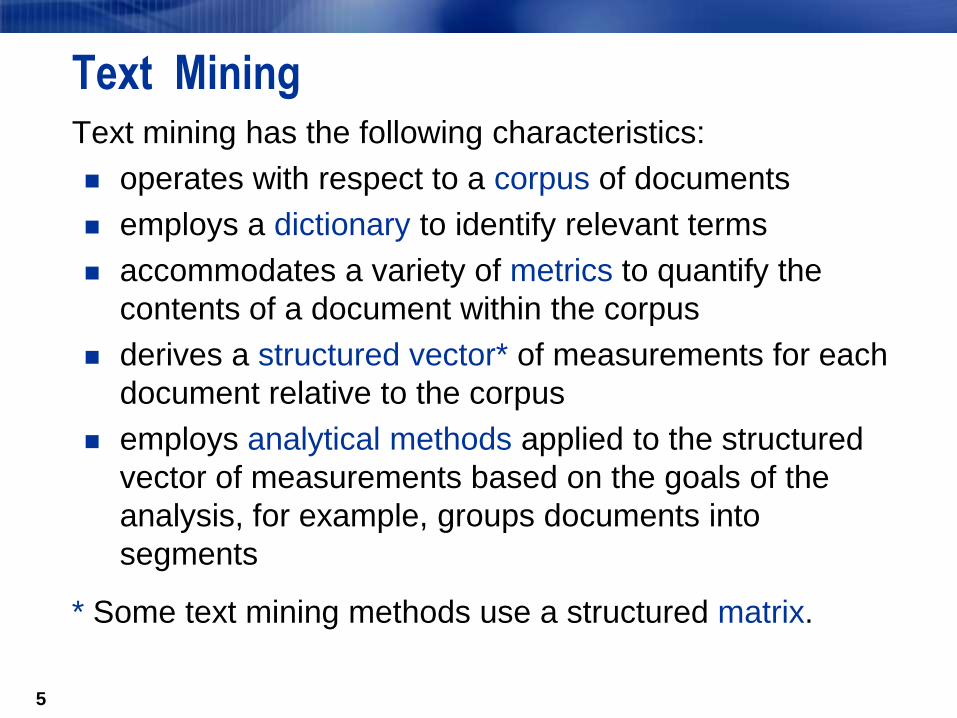
Text MiningText mining has the following characteristics:
operates with respect to a corpus of documents
employs a dictionary to identify relevant terms
accommodates a variety of metrics to quantify the
contents of a document within the corpus
derives a structured vector* of measurements for each
document relative to the corpus
employs analytical methods applied to the structured
vector of measurements based on the goals of the
analysis, for example, groups documents into
segments
* Some text mining methods use a structured matrix.

66
Another View of Text Mining
Text
A
Miracle
Occurs
Numbers

7
Application: Document Classification
7
New
Document
Group A vs. Others
Group B vs. Others
Group C vs. OthersGroup C
Group A
Group B

8
Document Categorization
Document categorization
Assign documents to pre-defined categories
Examples
Process email into work, personal, junk
Process documents from a newsgroup into “interesting”,
“not interesting”, “spam and flames”
Process transcripts of bugged phone calls into “relevant”
and “irrelevant”

9
Application: Information Retrieval
9
Document Collection
Text MiningInput
Document
Matched
Documents

10
IntroductionHow can we retrieve information using a search engine?.
We can represent the query and the documents as
vectors (vector space model)
– However to construct these vectors we should
perform a preliminary document preparation.
The documents are retrieved by finding the closest
distance between the query and the document vector.

11
Application: Clustering
11
Document Collection
Text Mining
Group
1Group 2 Group 3 Group 4

1212
SAS Text
Miner
...

13
Document Classification
Document classification
Cluster documents based on similarity
Examples
Group samples of writing in an attempt to determine
author(s)
Look for “hot spots” in customer feedback
Find new trends in a document collection (outliers,
hard to classify)

14
IR Applications Using Text Mining Survey Analysis
Analysis of Student Evaluations of Instructors
Predictive Modeling
Enrollment Models
Retention Models
14

1515
Predictive Modeling
Input X1
Text
Input X2
Input Xk
Pre-processing
Parsing
Transformation
Input T1
Input T2
Input Tj
Model Score
Cleaning
Screening
Derivation
Transformation
Imputation

1616
Obtaining the Prediction
Nominal Target
Binary/Categorical
Data
Model
Score
Rule
Prediction
Example
Binary Response: Mail (Y/N)
Age=33,Gender=F,Income=$45,000
g(Y)=f(Age,Gender,Income)
0.378
If (Score>0.255)
then Mail=Y

17
Objectives Explore the general concept of decision trees.
Build a decision tree model.
Examine the model results and interpret these results.

18
Fitted Decision Tree
New CaseDEBTINC = 20
PROPERTY VALUE = $500,000
DELINQUENCIES = 0
FIRST MORTGAGE = $200,000
Delinquencies
DEBTINC45
...
64%
0
1
<45
7%Property Value
< $300,000
$300,0006%
79%
Delinquencies
<6
6%
6
100%
First Mortgage
< $246,000 $246,000
92% 20%
Oldest Loan83%
53%
178< 178
64% 32%

19
The Cultivation of Trees Split Search
– Which splits are to be considered?
Splitting Criterion
– Which split is best?
Stopping Rule
– When should the splitting stop?
Pruning Rule
– Should some branches be lopped off?

20
Benefits of Trees Interpretability
– tree-structured presentation
Mixed Measurement Scales
– nominal, ordinal, interval
Regression trees
Robustness
Missing Values

21
Simple Prediction Illustration
0.0 0.50.1 0.2 0.3 0.4 0.6 0.7 0.8 0.9 1.0
0.0
0.5
0.1
0.2
0.3
0.4
0.6
0.7
0.8
0.9
1.0
x1
x2
Predict dot color
for each x1 and x2.
Training Data
...

22
Simple Prediction Illustration
0.0 0.50.1 0.2 0.3 0.4 0.6 0.7 0.8 0.9 1.0
0.0
0.5
0.1
0.2
0.3
0.4
0.6
0.7
0.8
0.9
1.0
x1
x2
Predict dot color
for each x1 and x2.
Training Data
...

23
Decision Tree Prediction Rules
0.0 0.50.1 0.2 0.3 0.4 0.6 0.7 0.8 0.9 1.0
0.0
0.5
0.1
0.2
0.3
0.4
0.6
0.7
0.8
0.9
1.0
x1
x2
40%
60%
55%
70%
x1
<0.52 ≥0.52 <0.51 ≥0.51x1
x2
<0.63 ≥0.63
root node
interior node
leaf node
...

24
Decision Tree Prediction Rules
0.0 0.50.1 0.2 0.3 0.4 0.6 0.7 0.8 0.9 1.0
0.0
0.5
0.1
0.2
0.3
0.4
0.6
0.7
0.8
0.9
1.0
x1
x2
40%
60%
55%
x1
<0.52 ≥0.52
<0.63
70%
<0.51 ≥0.51x1
x2
≥0.63
root node
interior node
leaf node
Predict:
...

25
≥0.51
40%
60%
55%
x1
<0.52 ≥0.52
<0.63
40%
60%
55%
x1
<0.52 ≥0.52 ≥0.51
<0.63
Decision Tree Prediction Rules
0.0 0.50.1 0.2 0.3 0.4 0.6 0.7 0.8 0.9 1.0
0.0
0.5
0.1
0.2
0.3
0.4
0.6
0.7
0.8
0.9
1.0
x1
x2
Decision =
Estimate = 0.70
70%
<0.51x1
x2
≥0.63
Predict:
...

26
Decision Tree Prediction Rules
40%
60%
55%
x1
<0.52 ≥0.52 ≥0.51
<0.63
0.0 0.50.1 0.2 0.3 0.4 0.6 0.7 0.8 0.9 1.0
0.0
0.5
0.1
0.2
0.3
0.4
0.6
0.7
0.8
0.9
1.0
x1
x2
Decision =
Estimate = 0.70
70%
<0.51x1
x2
≥0.63
Predict:
...

27
Decision Tree Split Search
0.0 0.50.1 0.2 0.3 0.4 0.6 0.7 0.8 0.9 1.0
x1
0.0
0.5
0.1
0.2
0.3
0.4
0.6
0.7
0.8
0.9
1.0
x2
Calculate the logworth
of every partition on
input x1.
left right
...
Confusion Matrix

28
Decision Tree Split Search
Calculate the logworth
of every partition on
input x1.
left right
...
Confusion Matrix
0.0 0.50.1 0.2 0.3 0.4 0.6 0.7 0.8 0.9 1.0
0.0
0.5
0.1
0.2
0.3
0.4
0.6
0.7
0.8
0.9
1.0
x1
x2
0.52

29
Decision Tree Split Search
0.0 0.50.1 0.2 0.3 0.4 0.6 0.7 0.8 0.9 1.0
0.0
0.5
0.1
0.2
0.3
0.4
0.6
0.7
0.8
0.9
1.0
x1
x2
max
logworth(x1)
0.95
0.52left right
Select the partition with
the maximum logworth.
53%
47%
42%
58%
...
30
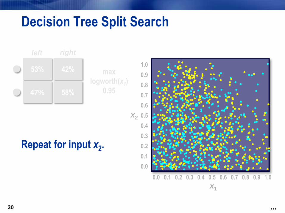
Decision Tree Split Search
0.0 0.50.1 0.2 0.3 0.4 0.6 0.7 0.8 0.9 1.0
0.0
0.5
0.1
0.2
0.3
0.4
0.6
0.7
0.8
0.9
1.0
x1
x2
max
logworth(x1)
0.95
left right
53% 42%
47% 58%
Repeat for input x2.
...

31
Decision Tree Split Search
0.0 0.50.1 0.2 0.3 0.4 0.6 0.7 0.8 0.9 1.0
0.0
0.5
0.1
0.2
0.3
0.4
0.6
0.7
0.8
0.9
1.0
x1
x2
max
logworth(x1)
0.95
left right
53% 42%
47% 58%
bottom top
...

32
Decision Tree Split Search
max
logworth(x1)
0.95
left right
53% 42%
47% 58%
0.0 0.50.1 0.2 0.3 0.4 0.6 0.7 0.8 0.9 1.0
0.0
0.5
0.1
0.2
0.3
0.4
0.6
0.7
0.8
0.9
1.0
x1
x2
0.63
max
logworth(x2)
4.92
bottom top
54%
46%
35%
65%
...

33
Decision Tree Split Search
0.0 0.50.1 0.2 0.3 0.4 0.6 0.7 0.8 0.9 1.0
0.0
0.5
0.1
0.2
0.3
0.4
0.6
0.7
0.8
0.9
1.0
x1
x2
max
logworth(x2)
4.92
bottom top
max
logworth(x1)
0.95
left right
Compare partition
logworth ratings.54%
46%
35%
65%
53%
47%
42%
58%
...

34
Decision Tree Split Search
max
logworth(x1)
0.95
left right
53% 42%
47% 58%
0.0 0.50.1 0.2 0.3 0.4 0.6 0.7 0.8 0.9 1.0
0.0
0.5
0.1
0.2
0.3
0.4
0.6
0.7
0.8
0.9
1.0
x1
x2
0.63
max
logworth(x2)
4.92
bottom top
54%
46%
35%
65%
...

35
Decision Tree Split Search
0.0 0.50.1 0.2 0.3 0.4 0.6 0.7 0.8 0.9 1.0
0.0
0.5
0.1
0.2
0.3
0.4
0.6
0.7
0.8
0.9
1.0
x1
x2
0.63
x2<0.63 ≥0.63
Create a partition rule
from the best partition
across all inputs.
...

36
Decision Tree Split Search
0.0 0.50.1 0.2 0.3 0.4 0.6 0.7 0.8 0.9 1.0
0.0
0.5
0.1
0.2
0.3
0.4
0.6
0.7
0.8
0.9
1.0
x1
x2
x2<0.63 ≥0.63
Repeat the process
in each subset.
...
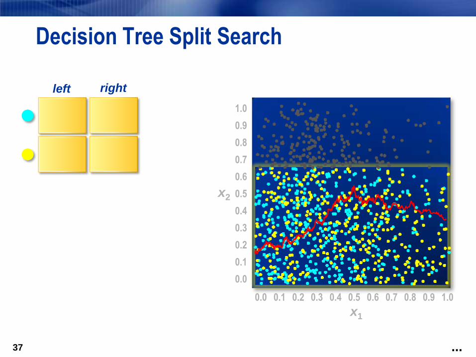
37
Decision Tree Split Search
0.0 0.50.1 0.2 0.3 0.4 0.6 0.7 0.8 0.9 1.0
0.0
0.5
0.1
0.2
0.3
0.4
0.6
0.7
0.8
0.9
1.0
x1
x2
left right
...

38
Decision Tree Split Search
0.0 0.50.1 0.2 0.3 0.4 0.6 0.7 0.8 0.9 1.0
0.0
0.5
0.1
0.2
0.3
0.4
0.6
0.7
0.8
0.9
1.0
x1
x2
0.52
max
logworth(x1)
5.72
left right
61%
39%
55%
45%
...

39
Decision Tree Split Search
0.0 0.50.1 0.2 0.3 0.4 0.6 0.7 0.8 0.9 1.0
0.0
0.5
0.1
0.2
0.3
0.4
0.6
0.7
0.8
0.9
1.0
x1
x2
max
logworth(x1)
5.72
left right
61% 55%
39% 45%
bottom top
...

40
Decision Tree Split Search
0.0 0.50.1 0.2 0.3 0.4 0.6 0.7 0.8 0.9 1.0
0.0
0.5
0.1
0.2
0.3
0.4
0.6
0.7
0.8
0.9
1.0
x1
x2
max
logworth(x1)
5.72
left right
61% 55%
39% 45%
0.02
max
logworth(x2)
-2.01
bottom top
38%
62%
55%
45%
...

41
Decision Tree Split Search
0.0 0.50.1 0.2 0.3 0.4 0.6 0.7 0.8 0.9 1.0
0.0
0.5
0.1
0.2
0.3
0.4
0.6
0.7
0.8
0.9
1.0
x1
x2
max
logworth(x2)
-2.01
bottom top
38%
62%
55%
45%
max
logworth(x1)
5.72
left right
61%
39%
55%
45%
...

42
Decision Tree Split Search
0.0 0.50.1 0.2 0.3 0.4 0.6 0.7 0.8 0.9 1.0
0.0
0.5
0.1
0.2
0.3
0.4
0.6
0.7
0.8
0.9
1.0
x1
x2
0.52
max
logworth(x2)
-2.01
bottom top
38% 55%
62% 45%
max
logworth(x1)
5.72
left right
61%
39%
55%
45%
...

43
Decision Tree Split Search
0.0 0.50.1 0.2 0.3 0.4 0.6 0.7 0.8 0.9 1.0
0.0
0.5
0.1
0.2
0.3
0.4
0.6
0.7
0.8
0.9
1.0
x1
x2
x2
x1
<0.63 ≥0.63
<0.52 ≥0.52
Create a second
partition rule.
...

44
Decision Tree Split Search
0.0 0.50.1 0.2 0.3 0.4 0.6 0.7 0.8 0.9 1.0
0.0
0.5
0.1
0.2
0.3
0.4
0.6
0.7
0.8
0.9
1.0
x1
x2
x2
x1
<0.63 ≥0.63
<0.52 ≥0.52
Create a second
partition rule.
...

45
Repeat to form a maximal tree.
Decision Tree Split Search
0.0 0.50.1 0.2 0.3 0.4 0.6 0.7 0.8 0.9 1.0
0.0
0.5
0.1
0.2
0.3
0.4
0.6
0.7
0.8
0.9
1.0
x1
x2
...

46
Example Two Year School on Texas & Mexico Border
Strong in Mathematics and Sciences
Weak in the Arts
Half of the students are from newly emigrated families
46

47
Improve Graduation Rate
Identify Students Most Likely Not to Graduate
Collect Data and Build a Predictive Model
Determine What Intervention is Approximate
47
Objective

48
Sample of 1000 Students Entering Fall 2010
Determine Which Students Had Left by Fall 2013
Data Fields
1. Student ID
2. Age
3. Gender
4. Major
5. Population
6. School
7. Enrollment Statement
8. Target
48
Hypothetical Data

49
49
Hypothetical Data

5050

5151

5252
Process Flow

5353
Decision Tree Model

5454
Fit Statistics

5555
ROC Curve

56
Score Students Entering in Fall 2013 With Model
Distribute Scoring Information to Approximate People
Evaluate Model After Two Years
56
Next Steps