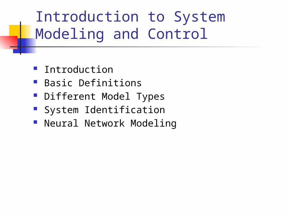
Introduction to System Modeling and Control

Introduction Basic Definitions Different Model Types System Identification Neural Network Modeling

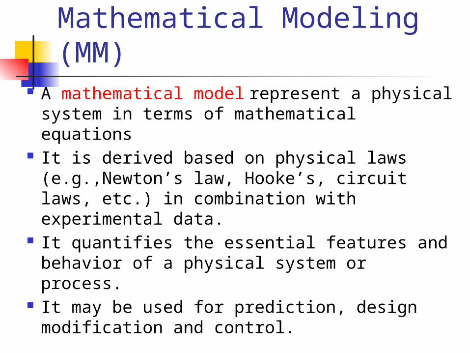
Mathematical Modeling (MM)

A mathematical model represent a physical system in terms of mathematical equations

It is derived based on physical laws (e.g.,Newton’s law, Hooke’s, circuit laws, etc.) in combination with experimental data.

It quantifies the essential features and behavior of a physical system or process.

It may be used for prediction, design modification and control.

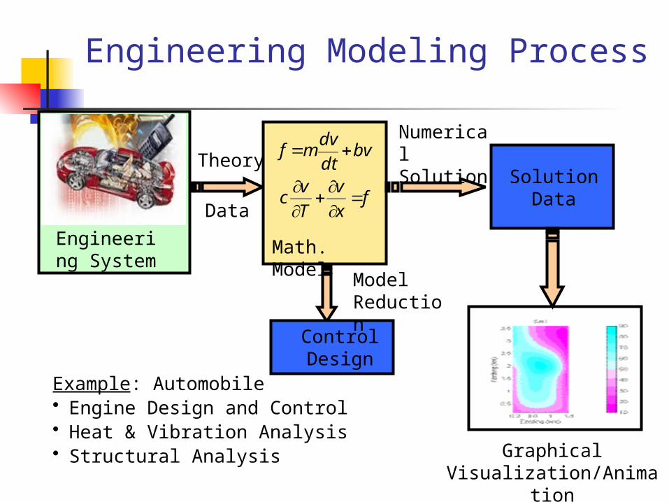
Engineering Modeling Process

Graphical Visualization/Animation

Engineering System

Theory

Data

Example: Automobile• Engine Design and Control• Heat & Vibration Analysis• Structural Analysis

Solution Data

Math. Model

fx

v

T

vc

bvdt

dvmf

Numerical Solution

Control Design

Model Reduction

Definition of System

System: An aggregation or assemblage of things so combined by man or nature to form an integral and complex whole.

From engineering point of view, a system is defined as an interconnection of many components or functional units act together to perform a certain objective, e.g., automobile, machine tool, robot, aircraft, etc.

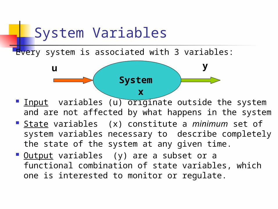
System VariablesEvery system is associated with 3 variables:

Input variables (u) originate outside the system and are not affected by what happens in the system

State variables (x) constitute a minimum set of system variables necessary to describe completely the state of the system at any given time.

Output variables (y) are a subset or a functional combination of state variables, which one is interested to monitor or regulate.

Systemu y

x

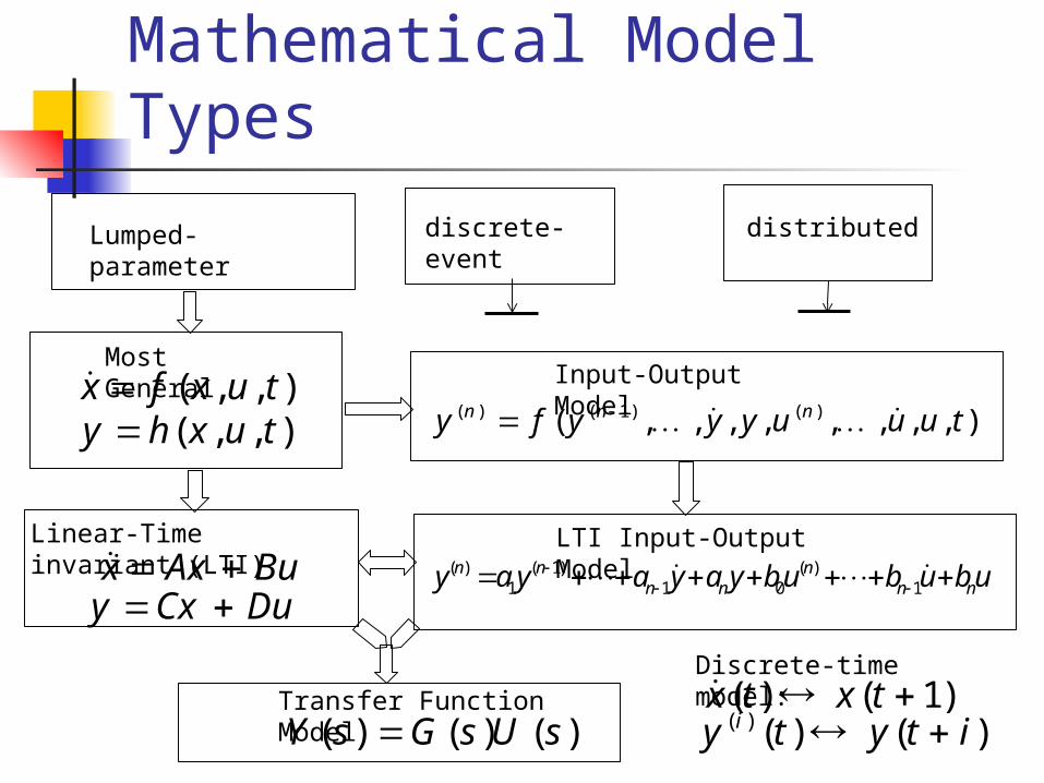
Mathematical Model Types

Lumped-parameter

discrete-event

Most General ),,( tuxfx

),,( tuxhy

Linear-Time invariant (LTI)

DuCxy BuAxx

Input-Output Model ),,,,,,,,( )()1()( tuuuyyyfy nnn

distributed

LTI Input-Output Model

ubububyayayay nnn

nnnn 1

)(01

)1(1

)(

Transfer Function Model)()()( sUsGsY

Discrete-time model:

)()()( ityty i )1()( txtx

Example: Accelerometer (Text 6.6.1)

Consider the mass-spring-damper (may be used as accelerometer or seismograph) system shown below:

Free-Body-Diagram

M

fs

fd

fs

fd

x

fs(y): position dependent spring force, y=u-xfd(y): velocity dependent spring force

Newton’s 2nd law )()( yfyfyuMxM sd

Linearizaed model: uMkyybyM

M

ux

Example II: Delay Feedback

Delayz -1

u y

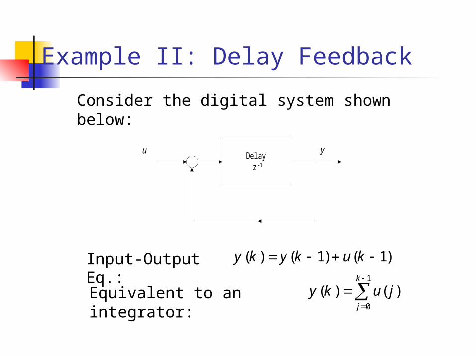
Consider the digital system shown below:

Input-Output Eq.: )1()1()( kukyky

Equivalent to an integrator:

1

0

)()(k

j

juky

Transfer Function

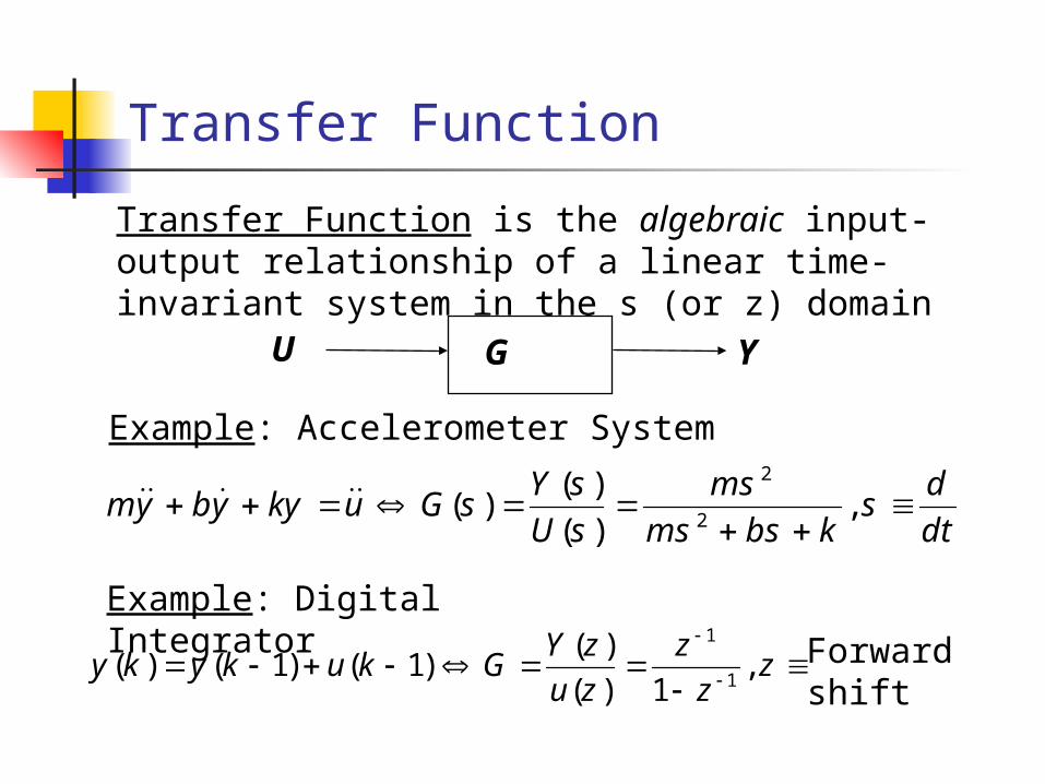
Transfer Function is the algebraic input-output relationship of a linear time-invariant system in the s (or z) domain

GU Y

dt

ds

kbsms

ms

sU

sYsGukyybym

,

)(

)()(

2

2

Example: Accelerometer System

Example: Digital Integrator

zz

z

zu

zYGkukyky ,

1)(

)()1()1()(

1

1Forward shift

Comments on TF

Transfer function is a property of the system independent from input-output signal

It is an algebraic representation of differential equations

Systems from different disciplines (e.g., mechanical and electrical) may have the same transfer function

Acceleromter Transfer Function

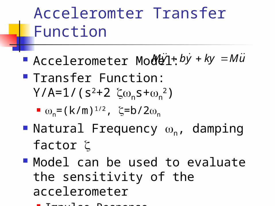
Accelerometer Model: Transfer Function:

Y/A=1/(s2+2ns+n2) n=(k/m)1/2, =b/2n

Natural Frequency n, damping factor

Model can be used to evaluate the sensitivity of the accelerometer Impulse Response Frequency Response

uMkyybyM

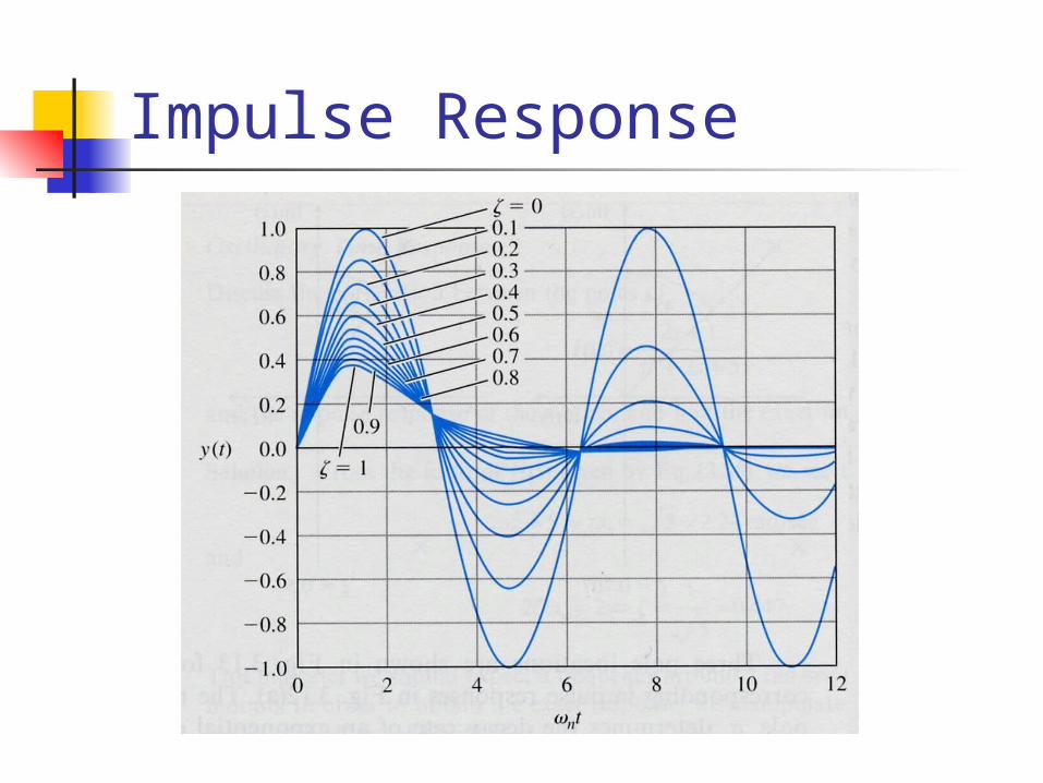
Impulse Response

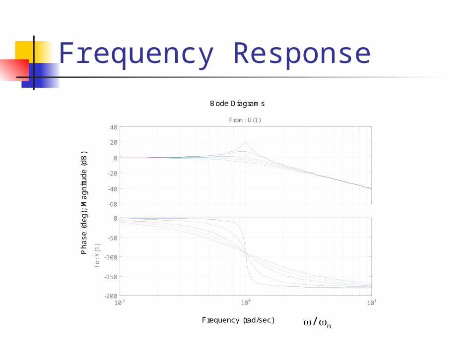
Frequency Response

Frequency (rad/sec)

Ph

as

e (

de

g);

Ma

gn

itu

de

(d

B)

Bode Diagrams

-60

-40

-20

0

20

40From: U(1)

10-1 100 101-200

-150

-100

-50

0

To

: Y

(1)

/n

Mixed Systems

Most systems in mechatronics are of the mixed type, e.g., electromechanical, hydromechanical, etc

Each subsystem within a mixed system can be modeled as single discipline system first

Power transformation among various subsystems are used to integrate them into the entire system

Overall mathematical model may be assembled into a system of equations, or a transfer function

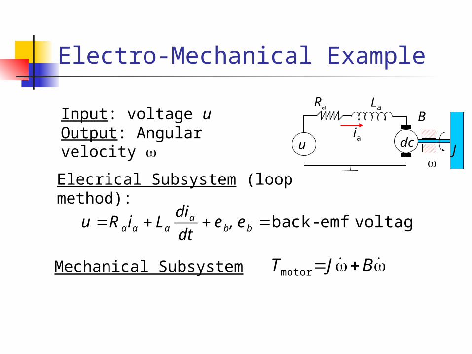
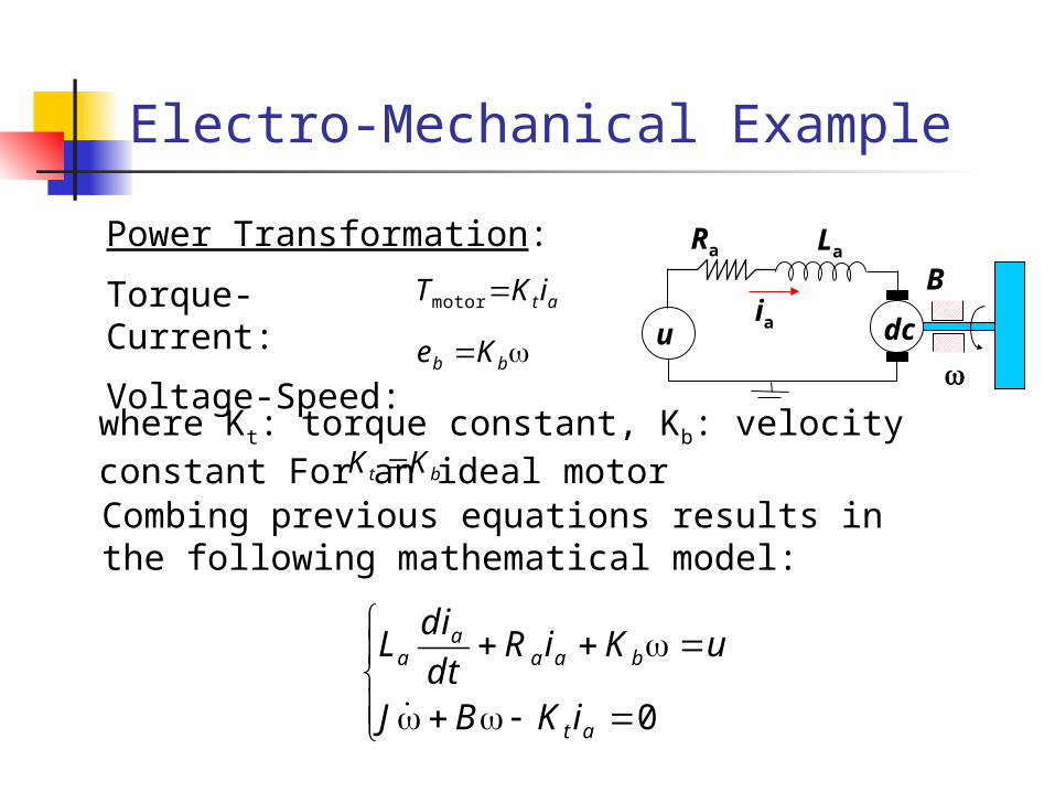
Electro-Mechanical Example

voltage emf-back bba

aaa e,edt

diLiRu

Mechanical Subsystem BJTmotor

uia dc

Ra La

J

BInput: voltage uOutput: Angular velocity

Elecrical Subsystem (loop method):

Electro-Mechanical Example

Torque-Current:

Voltage-Speed:

at iKT motor

Combing previous equations results in the following mathematical model:

uia dc

Ra La

B

Power Transformation:

bb Ke

0at

baaa

a

iKBJ

uKiRdt

diL

where Kt: torque constant, Kb: velocity constant For an ideal motor bt KK

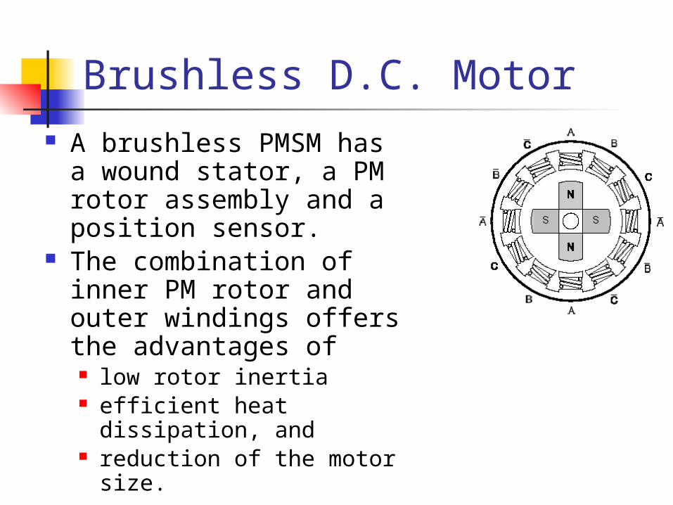
Brushless D.C. Motor A brushless PMSM has a

wound stator, a PM rotor assembly and a position sensor.

The combination of inner PM rotor and outer windings offers the advantages of low rotor inertia efficient heat dissipation, and reduction of the motor size.

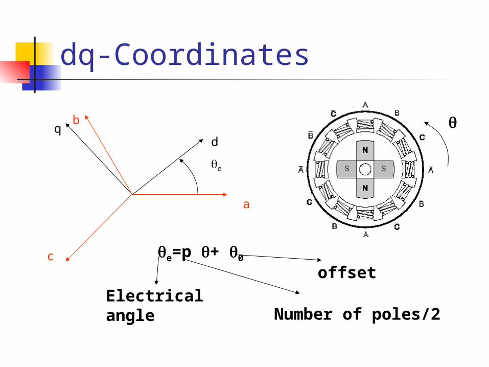
dq-Coordinates

a

qb

c

d

e

e=p + 0

Electrical angleNumber of poles/2

offset

Mathematical Model

qme

dmqq

dqmdd

vLL

Kipi

L

R

dt

di

vL

ipiL

R

dt

di

1

1

Where p=number of poles/2, Ke=back emf constant

qtem iKTJ

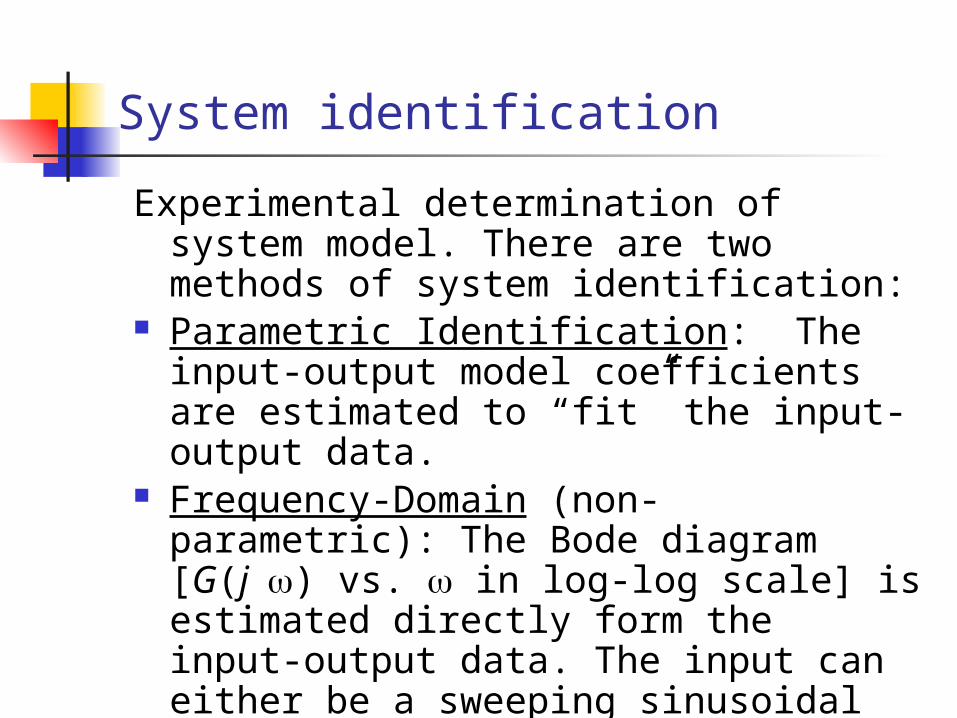
System identification

Experimental determination of system model. There are two methods of system identification:

Parametric Identification: The input-output model coefficients are estimated to “fit” the input-output data.

Frequency-Domain (non-parametric): The Bode diagram [G(j) vs. in log-log scale] is estimated directly form the input-output data. The input can either be a sweeping sinusoidal or random signal.

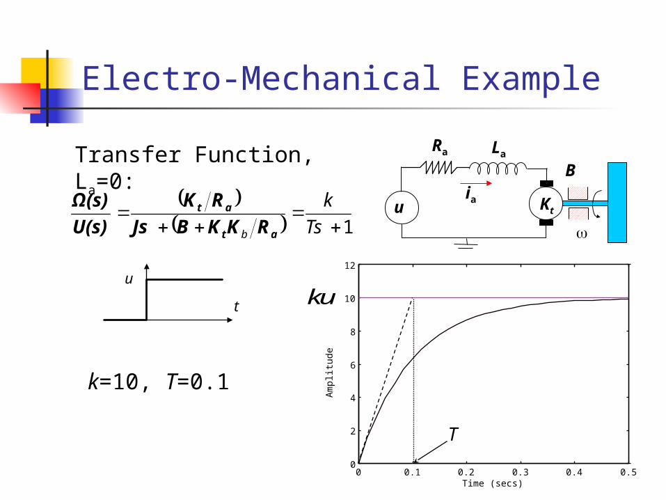
Electro-Mechanical Example

uia Kt

Ra La

B

1

Ts

k

b at

at

RKKBJs

RK

U(s)

Ω(s)

Transfer Function, La=0:

0 0.1 0.2 0.3 0.4 0.50

2

4

6

8

10

12

Time (secs)

Am

plitu

de

ku

T

u

t

k=10, T=0.1

Comments on First Order Identification

Graphical method is difficult to optimize with noisy data

and multiple data sets only applicable to low order

systems difficult to automate

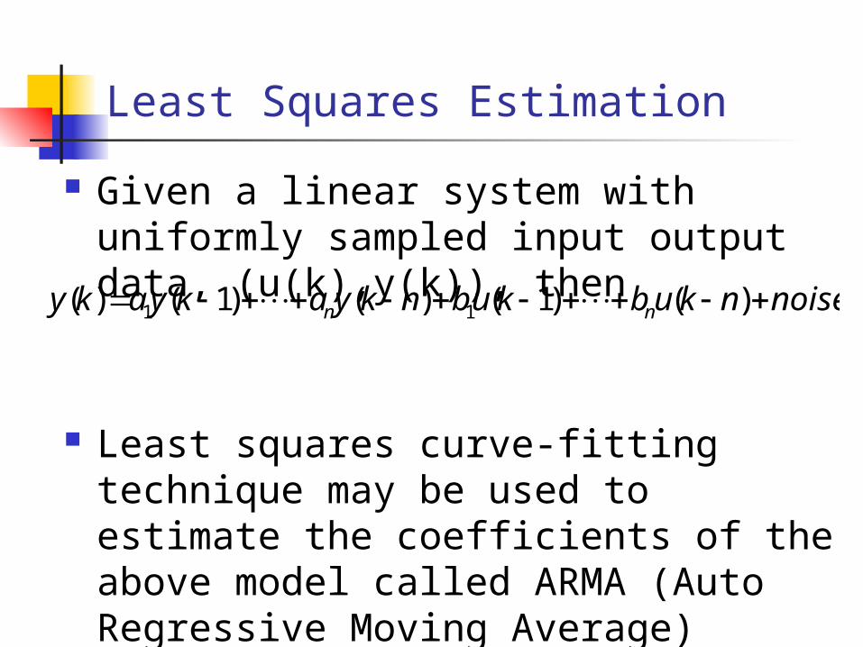
Least Squares Estimation

Given a linear system with uniformly sampled input output data, (u(k),y(k)), then

Least squares curve-fitting technique may be used to estimate the coefficients of the above model called ARMA (Auto Regressive Moving Average) model.

noisenkubkubnkyakyaky nn )()1()()1()( 11

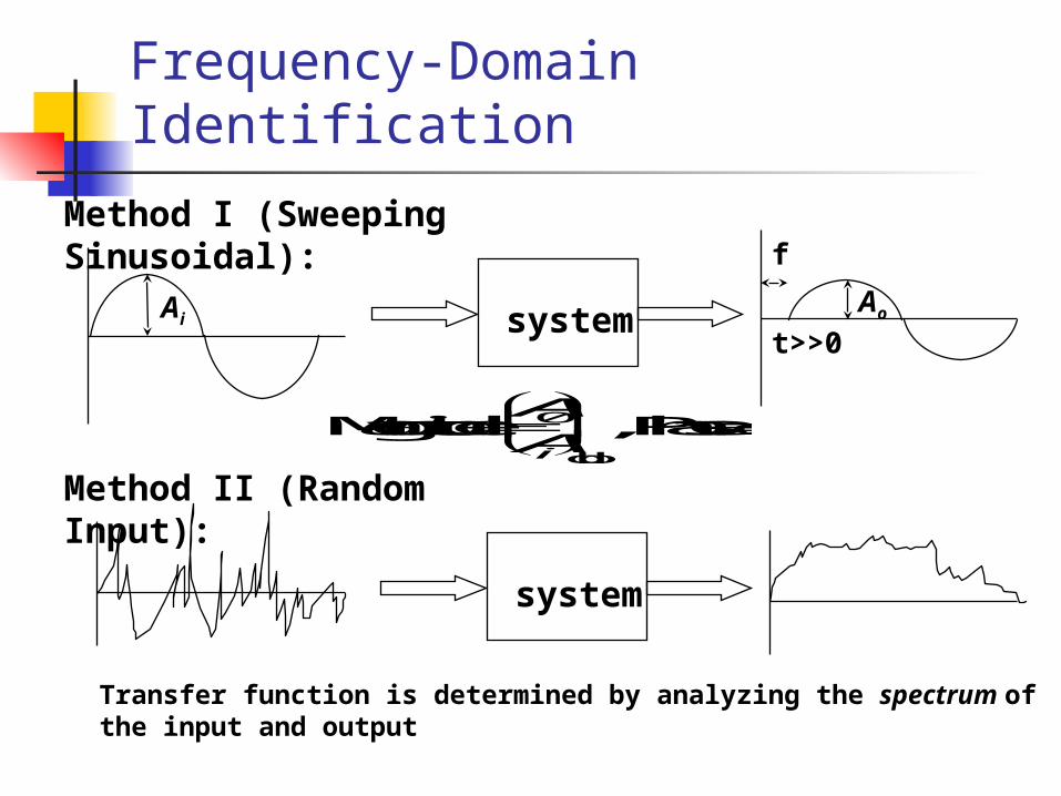
Frequency-Domain Identification

Method I (Sweeping Sinusoidal):

systemAiAo

f

t>>0

Magnitude Phasedb

A

Ai

0 ,

Method II (Random Input):

system

Transfer function is determined by analyzing the spectrum of the input and output

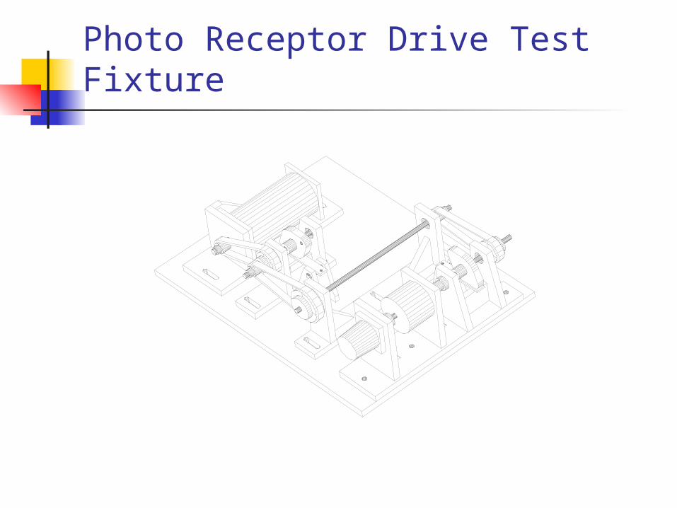
Photo Receptor Drive Test Fixture

Experimental Bode Plot

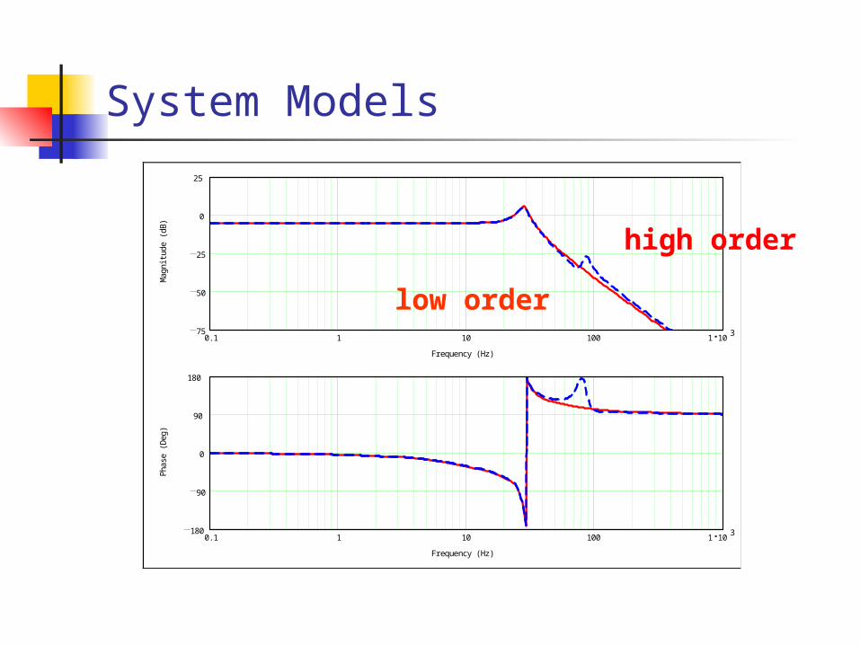
System Models

0.1 1 10 100 1 10375

50

25

0

25

Frequency (Hz)

Ma

gn

itu

de

(d

B)

0.1 1 10 100 1 103180

90

0

90

180

Frequency (Hz)

Ph

ase

(D

eg

)

high order

low order

Nonlinear System Modeling& Control

Neural Network Approach

Introduction Real world nonlinear systems often difficult to

characterize by first principle modeling First principle models are often

suitable for control design Modeling often accomplished with input-

output maps of experimental data from the system

Neural networks provide a powerful tool for data-driven modeling of nonlinear systems

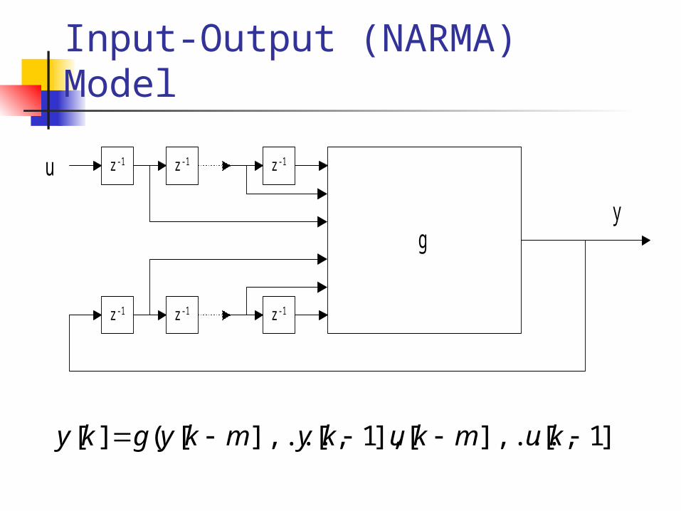
Input-Output (NARMA) Model

])1[],...,[],1[],...,[(][ kumkukymkygky

g

z -1 z -1 z -1

z -1 z -1 z -1

u

y

What is a Neural Network?

Artificial Neural Networks (ANN) are massively parallel computational machines (program or hardware) patterned after biological neural nets.

ANN’s are used in a wide array of applications requiring reasoning/information processing including pattern recognition/classification monitoring/diagnostics system identification & control forecasting optimization

Advantages and Disadvantages of ANN’s

Advantages: Learning from Parallel architecture Adaptability Fault tolerance and redundancy

Disadvantages: Hard to design Unpredictable behavior Slow Training “Curse” of dimensionality

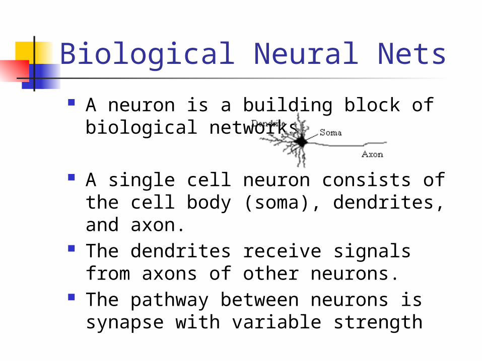
Biological Neural Nets A neuron is a building block of biological

networks

A single cell neuron consists of the cell body (soma), dendrites, and axon.

The dendrites receive signals from axons of other neurons.

The pathway between neurons is synapse with variable strength

Artificial Neural Networks

They are used to learn a given input-output relationship from input-output data (exemplars).

The neural network type depends primarily on its activation function

Most popular ANNs: Sigmoidal Multilayer Networks Radial basis function NLPN (Sadegh et al 1998,2010)

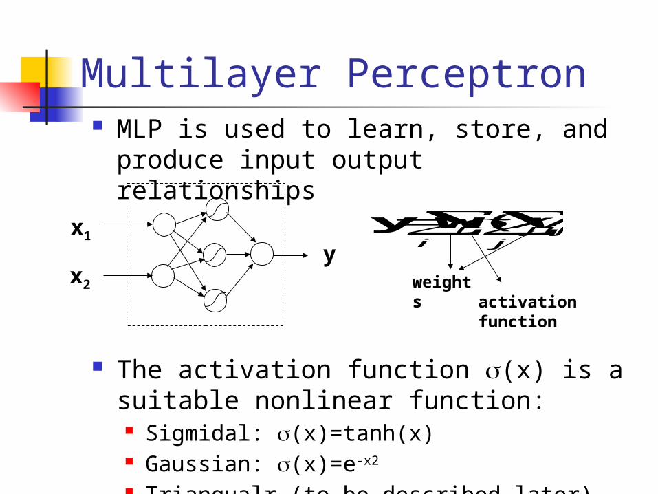
Multilayer Perceptron MLP is used to learn, store, and produce

input output relationships

The activation function (x) is a suitable nonlinear function: Sigmidal: (x)=tanh(x) Gaussian: (x)=e-x2

Triangualr (to be described later)

x1

x2

y

)( ijj

ji

i vx wy

weightsactivation function

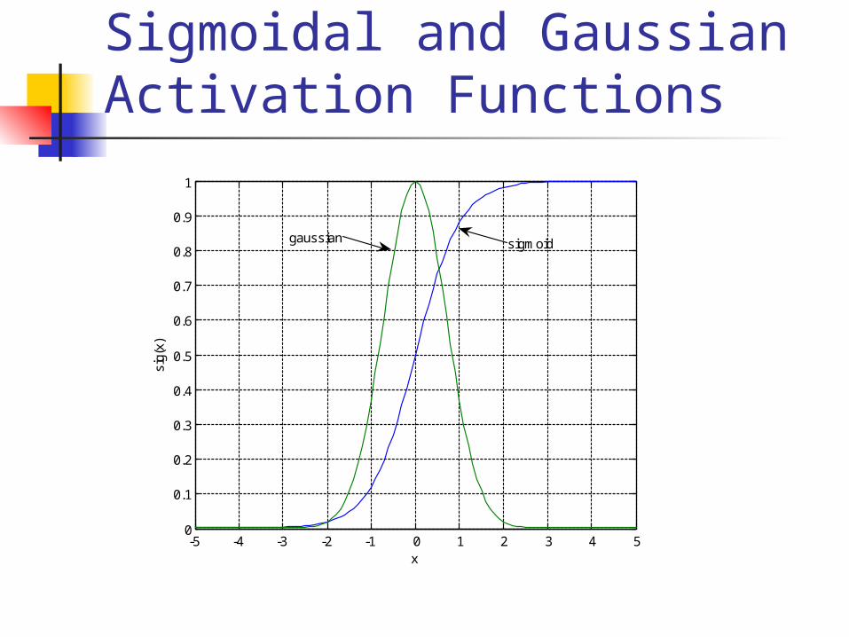
Sigmoidal and Gaussian Activation Functions

-5 -4 -3 -2 -1 0 1 2 3 4 50

0.1

0.2

0.3

0.4

0.5

0.6

0.7

0.8

0.9

1

x

sig(

x)

gaussian sigmoid

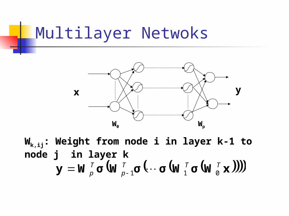
Multilayer Netwoks

Wk,ij: Weight from node i in layer k-1 to node j in layer k

xWσWσσWσWy TTTp

Tp 011

x y

W0 Wp

Universal Approximation Theorem (UAT)

Comments: The UAT does not say how large the

network should be Optimal design and training may be

difficult

A single hidden layer perceptron network with a sufficiently large number of neurons can approximate any continuous function arbitrarily close.

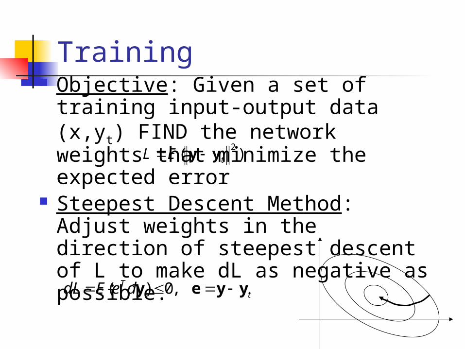
Training Objective: Given a set of training

input-output data (x,yt) FIND the network weights that minimize the expected error

Steepest Descent Method: Adjust weights in the direction of steepest descent of L to make dL as negative as possible.

)(2

tEL yy

tTdeEdL yyey ,0)(

Neural Network Approximation of NARMA Model

y

y[k-m]

u[k-1]

Question: Is an arbitrary neural network model consistent with a physical system (i.e., one that has an internal realization)?

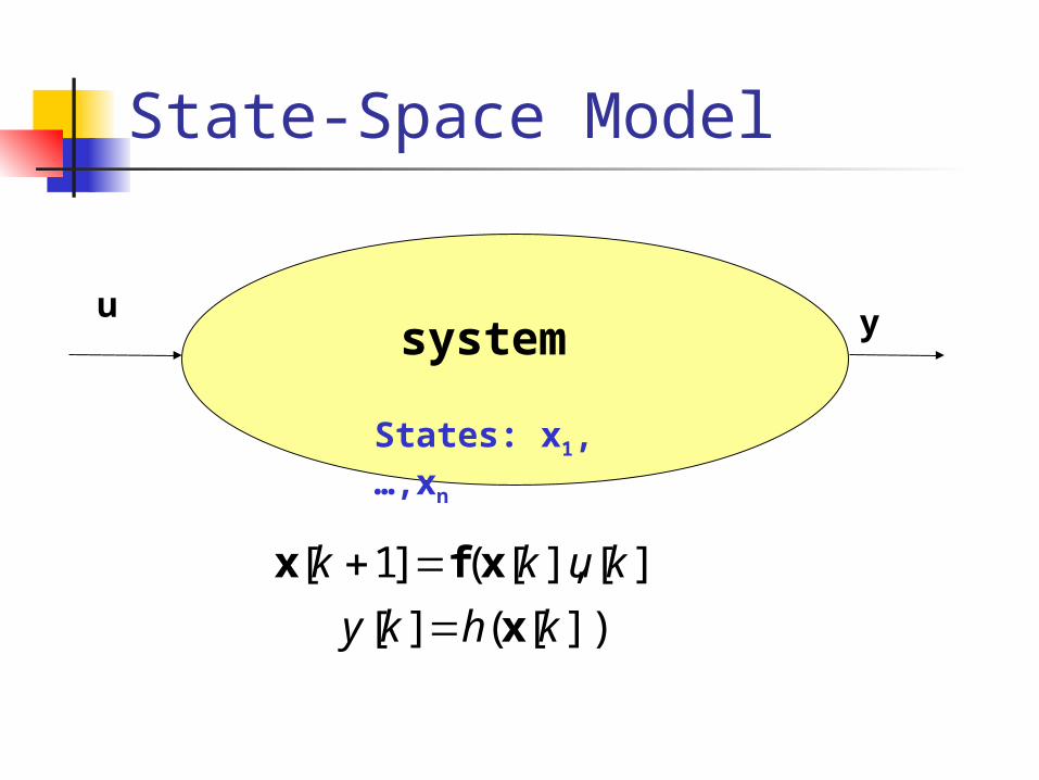
State-Space Model

])[(][

])[],[(]1[

khky

kukk

x

xfx

u y

States: x1,…,xn

system

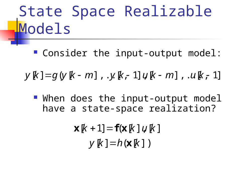
A Class of Observable State Space Realizable Models

Consider the input-output model:

When does the input-output model have a state-space realization?

])[(][

])[],[(]1[

khky

kukk

x

xfx

])1[],...,[],1[],...,[(][ kumkukymkygky

Comments on State Realization of Input-Output Model

A Generic input-Output Model does not necessarily have a state-space realization (Sadegh 2001, IEEE Trans. On Auto. Control)

There are necessary and sufficient conditions for realizability

Once these conditions are satisfied the state-space model may be symbolically or computationally constructed

A general class of input-Output Models may be constructed that is guaranteed to admit a state-space realization

Fluid Power Application

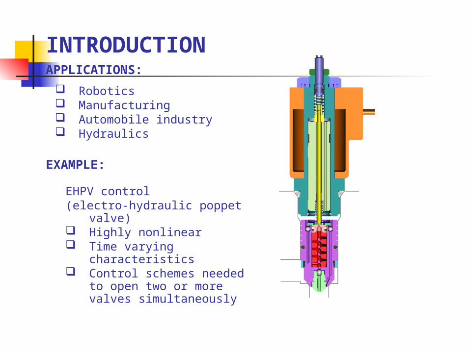
APPLICATIONS:

Robotics Manufacturing Automobile industry Hydraulics

INTRODUCTION

EHPV control(electro-hydraulic poppet valve) Highly nonlinear Time varying characteristics Control schemes needed to

open two or more valves simultaneously

EXAMPLE:

Motivation

The valve opening is controlled by means of the solenoid input current

The standard approach is to calibrate of the current-opening relationship for each valve

Manual calibration is time consuming and inefficient

Research Goals

Precisely control the conductivity of each valve using a nominal input-output relationship.

Auto-calibrate the input-output relationship

Use the auto-calibration for precise control without requiring the exact input-output relationship

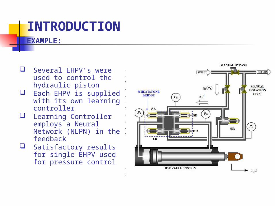
EXAMPLE:

Several EHPV’s were used to control the hydraulic piston

Each EHPV is supplied with its own learning controller

Learning Controller employs a Neural Network (NLPN) in the feedback

Satisfactory results for single EHPV used for pressure control

INTRODUCTION

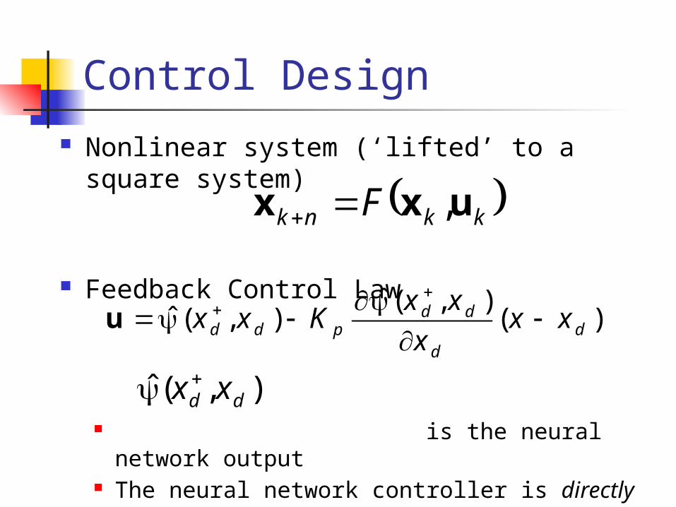
Control Design Nonlinear system (‘lifted’ to a square

system)

Feedback Control Law

is the neural network output The neural network controller is directly trained

based on the time history of the tracking error

kknk F uxx ,

)(),(ˆ

),(ˆ dd

ddpdd xx

x

xxKxx

u

),(ˆ dd xx

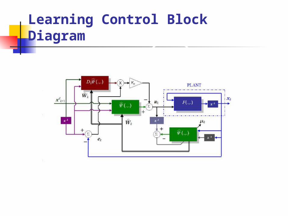
Learning Control Block Diagram

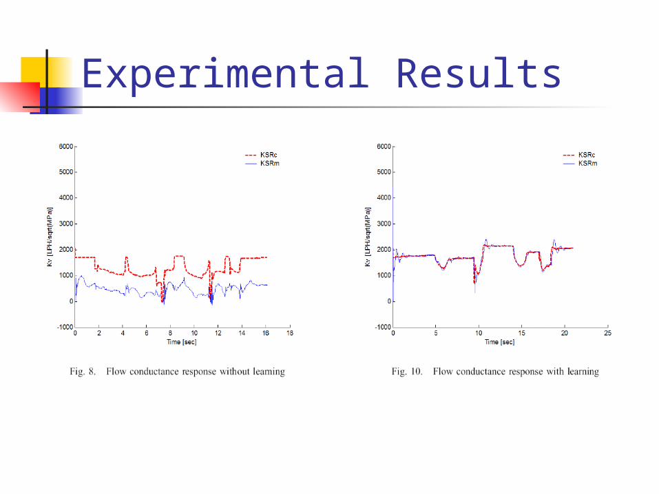
Experimental Results

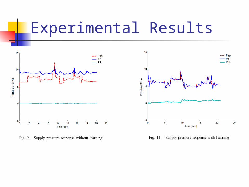
Experimental Results