Introduction to Stochastic Actor-Based Modelsfor Network Dynamics ∗

Tom A.B. Snijders†

Gerhard G. van de Bunt‡

Christian E.G. Steglich§

Abstract

Stochastic actor-based models are models for network dynamics that canrepresent a wide variety of influences on network change, and allow to es-timate parameters expressing such influences, and test corresponding hy-potheses. The nodes in the network represent social actors, and the collec-tion of ties represents a social relation. The assumptions posit that the net-work evolves as a stochastic process ‘driven by the actors’, i.e., the modellends itself especially for representing theories about how actors changetheir outgoing ties. The probabilities of tie changes are in part endogenouslydetermined, i.e., as a function of the current network structure itself, and inpart exogenously, as a function of characteristics of the nodes (‘actor covari-ates’) and of characteristics of pairs of nodes (‘dyadic covariates’). In anextended form, stochastic actor-based models can be used to analyze longi-tudinal data on social networks jointly with changing attributes of the actors:dynamics of networks and behavior.

This paper gives an introduction to stochastic actor-based models fordynamics of directed networks, using only a minimum of mathematics. Thefocus is on understanding the basic principles of the model, understandingthe results, and on sensible rules for model selection.

Keywords: statistical modeling, longitudinal, Markov chain, agent-based model,peer selection, peer influence.∗Draft article for special issue of Social Networks on Dynamics of Social Networks. We are

grateful to Andrea Knecht who collected the data used in the example, under the guidance of ChrisBaerveldt. We also are grateful to Matthew Checkley and two reviewers for their very helpfulremarks on earlier drafts.†University of Oxford and University of Groningen‡Free University, Amsterdam§University of Groningen

1

1. Introduction

Social networks are dynamic by nature. Ties are established, they may flourishand perhaps evolve into close relationships, and they can also dissolve quietly, orsuddenly turn sour and go with a bang. These relational changes may be con-sidered the result of the structural positions of the actors within the network –e.g., when friends of friends become friends–, characteristics of the actors (‘actorcovariates’), characteristics of pairs of actors (‘dyadic covariates’), and residualrandom influences representing unexplained influences. Social network researchhas in recent years paid increasing attention to network dynamics, as is shown,e.g., by the three special issues devoted to this topic in Journal of MathematicalSociology edited by Patrick Doreian and Frans Stokman (1996, 2001, and 2003;also see Doreian and Stokman, 1997). The three issues shed light on the under-lying theoretical micro mechanisms that induce the evolution of social networkstructures on the macro level. Network dynamics is important for domains rang-ing from friendship networks (e.g., Pearson and Michell, 2000; Burk, Steglich,and Snijders, 2007) to, for example, organizational networks (see the review ar-ticles Borgatti and Foster, 2003; Brass, Galaskiewicz, Greve, and Tsai, 2004).

In this article we give a tutorial introduction to what we call here stochas-tic actor-based models for network dynamics, which are a type of models thathave the purpose to represent network dynamics on the basis of observed longi-tudinal data, and evaluate these according to the paradigm of statistical inference.This means that the models should be able to represent network dynamics as be-ing driven by many different tendencies, such as the micro mechanisms alludedto above, which could have been theoretically derived and/or empirically estab-lished in earlier research, and which may well operate simultaneously. Some ex-amples of such tendencies are reciprocity, transitivity, homophily, and assortativematching, as will be elaborated below. In this way, the models should be ableto give a good representation of the stochastic dependence between the creation,and possibly termination, of different network ties. These stochastic actor-basedmodels allow to test hypotheses about these tendencies, and to estimate param-eters expressing their strengths, while controlling for other tendencies (which instatistical terminology might be called ‘confounders’).

The literature on network dynamics has generated a large variety of mathe-matical models. To describe the place in the literature of stochastic actor-basedmodels (Snijders 1996, 2001), these models may be contrasted with other dynamicnetwork models.

Most network dynamics models in the literature pay attention to a very spe-cific set of micro mechanisms –allowing detailed analyses of the properties ofthese models–, but lack an explicit estimation theory. Examples are models pro-

2

posed by Bala and Goyal (2000), Hummon (2000), Skyrms and Pemantle (2000),and Marsili, Vega-Redondo, and Slanina (2004), all being actor-based simulationmodels that focus on the expression of a single social theory as reflected, e.g., by asimple utility function; those proposed by Jin, Girvan, and Newman (2001) whichrepresent a larger but still quite restricted number of tendencies; and models suchas those proposed by Price (1976), Barabasi and Albert (1999), and Jackson andRogers (2007), which are actor-based, represent one or a restricted set of tenden-cies, and assume that nodes are added sequentially while existing ties cannot bedeleted, which is a severe limitation to the type of longitudinal data that may befaithfully represented. Since such models do not allow to control for other influ-ences on the network dynamics, and how to estimate and test parameters is notclear for them, they cannot be used for purposes of theory testing in a statisticalmodel.

The earlier literature does contain some statistical dynamic network mod-els, mainly those developed by Wasserman (1979) and Wasserman and Iacobucci(1988), but these do not allow complicated dependencies between ties such as aregenerated by transitive closure. Further there are papers that present an empiri-cal analysis of network dynamics which are based on intricate and illuminatingdescriptions such as Holme, Edling, and Liljeros (2004) and Kossinets and Watts(2006), but which are not based on an explicit stochastic model for the networkdynamics and therefore do not allow to control one tendency for other (‘confound-ing’) tendencies.

Distinguishing characteristics of stochastic actor-based models are flexibility,allowing to incorporate a wide variety of actor-driven micro mechanisms influ-encing tie formation; and the availability of procedures for estimating and testingparameters that also allow to assess the effect of a given mechanism while control-ling for the possible simultaneous operation of other mechanisms or tendencies.

We assume here that the empirical data consist of two, but preferably more,repeated observations of a social network on a given set of actors; one could callthis network panel data. Ties are supposed to be the dyadic constituents of rela-tions such as friendship, trust, or cooperation, directed from one actor to another.In our examples social actors are individuals, but they could also be firms, coun-tries, etc. The ties are supposed to be, in principle, under control of the send-ing actor (although this will be subject to constraints), which will exclude mosttypes of relations where negotiations are required for a tie to come into existence.Actor covariates may be constant like sex or ethnicity, or subject to change likeopinions, attitudes, or lifestyle behaviors. Actor covariates often are among thedeterminants of actor similarity (e.g., same sex or ethnicity) or spatial proximitybetween actors (e.g., same neighborhood) which influence the existence of ties.

3

Dyadic covariates likewise may be constant, such as determined by kinship orformal status in an organization, or changing over time, like friendship betweenparents of children or task dependencies within organizations.

This paper is organized as follows. In the next section, we present the assump-tions of the actor-based model. The heart of the model is the so-called objectivefunction, which determines probabilistically the tie changes made by the actors.One could say that it captures all theoretically relevant information the actorsneed to ‘evaluate’ their collection of ties. Some of the potential components ofthis function are structure-based (endogenous effects), such as the tendency toform reciprocal relations, others are attribute-based (exogenous effects), such asthe preference for similar others. In Section 3 we discuss several statistical is-sues, such as data requirements and how to test and select the appropriate model.Following this we present an example about friendship dynamics, focusing on theinterpretation of the parameters. Section 4 proposes some more elaborate models.In Section 5, models for the coevolution of networks and behavior are introducedand illustrated by an example. Section 6 discusses the difference between equilib-rium and out-of-equilibrium situations, and how these longitudinal models relateto cross-sectional statistical modeling of social networks. Finally, in Section 7, abrief discussion is given, the Siena software is mentioned which implements thesemethods, and some further developments are presented.

2. Model assumptions

A dynamic network consists of ties between actors that change over time. Afoundational assumption of the models discussed in this paper is that the networkties are not brief events, but can be regarded as states with a tendency to endureover time. Many relations commonly studied in network analysis naturally satisfythis requirement of gradual change, such as friendship, trust, and cooperation.Other networks more strongly resemble ‘event data’, e.g., the set of all telephonecalls among a group of actors at any given time point, or the set of all e-mails beingsent at any given time point. While it is meaningful to interpret these networks asindicators of communication, it is not plausible to treat their ties as enduring states,although it often is possible to aggregate event intensity over a certain period andthen view these aggregates as indicators of states.

Given that the network ties under study denote states, it is further assumed, asan approximation, that the changing network can be interpreted as the outcomeof a Markov process, i.e., that for any point in time, the current state of the net-work determines probabilistically its further evolution, and there are no additionaleffects of the earlier past. All relevant information is therefore assumed to be in-cluded in the current state. This assumption often can be made more plausible by

4

choosing meaningful independent variables that incorporate relevant informationfrom the past.

This paper gives a non-technical introduction into actor-based models for net-work dynamics. More precise explanations can be found in Snijders (2001, 2005)and Snijders, Steglich, and Schweinberger (2007). However, a modicum of math-ematical notation cannot be avoided. The tie variables are binary variables, de-noted by xij . A tie from actor i to actor j, denoted i → j, is either present orabsent (xij then having values 1 and 0, respectively). Although this is in line withtraditional network analysis, an extension to valued networks would often be the-oretically sound, and could make the Markov assumption more plausible. This isone of the topics of current research. The tie variables constitute the network, rep-resented by its n×n adjacency matrix x =

(xij

)(self-ties are excluded), where n

is the total number of actors. The changes in these tie variables are the dependentvariables in the analysis.

2.1. Basic assumptions

The model is about directed relations, where each tie i → j has a sender i, whowill be referred to as ego, and a receiver j, referred to as alter. The followingassumptions are made.

1. The underlying time parameter t is continuous, i.e., the process unfolds intime steps of varying length, which could be arbitrarily small. The param-eter estimation procedure, however, assumes that the network is observedonly at two or more discrete points in time. The observations can also bereferred to as ‘network panel waves’, analogous to panel surveys in non-network studies.

This assumption was proposed already by Holland and Leinhardt (1977),and elaborated by Wasserman (1979 and other publications) and Leenders(1995 and other publications) – but their models represented only reci-procity, and no other structural dependencies between network ties. Thecontinuous-time assumption allows to represent dependencies between net-work ties as the result of processes where one tie is formed as a reaction tothe existence of other ties. If, for example, three actors who at the first ob-servation are mutually disconnected form at the second observation a closedtriangle, where each is connected to both of the others, then a discrete-timemodel that has the observations as its time steps would have to account forthe fact that this closed triangle structure is formed ‘out of nothing’, in onetime step. In our model such a closed triangle can be formed tie by tie, as aconsequence of reciprocation and transitive closure. Thus, the appearance

5

of closed triangles may be explained based on reciprocity and transitive pro-cesses, without requiring a special process specifically for closed triangles.

Since many small changes can add up to large differences between con-secutively observed networks, this does not preclude that what is observedshows large changes from one observation to the next.

2. The changing network is the outcome of a Markov process. This was ex-plained above. Thus, the total network structure is the social context thatinfluences the probabilities of its own change.

The assumption of a Markov process has been made in practically all mod-els for social network dynamics, starting by Katz and Proctor’s (1959) dis-crete Markov chain model. This is an assumption that will usually not berealistic, but it is difficult to come up with manageable models that do notmake it. We could say that this assumption is a lens through which we lookat the data – it should help but it also may distort. If there are only two panelwaves, then the data have virtually no information to test this assumption.For more panel waves, there is in principle the possibility to test this as-sumption and propose models making less restrictive assumption about thetime dependence, but this will require quite complicated models.

3. The actors control their outgoing ties. This means not that actors can changetheir outgoing ties at will, but that changes in ties are made by the actorswho send the tie, on the basis of their and others’ attributes, their positionin the network, and their perceptions about the rest of the network. Thisassumption is the reason for using the term ‘actor-based model’. This ap-proach to modeling is in line with the methodological approach of structuralindividualism (Udehn, 2002; Hedstrom, 2005), where actors are assumed tobe purposeful and to behave subject to structural constraints. The assump-tion of purposeful actors is not required, however, but a question of modelinterpretation (see below).It is assumed formally that actors have full information about the networkand the other actors. In practice, as can be concluded from the specifica-tions given below, the actors only need more limited information, becausethe probabilities of network changes by an actor depend on the personal net-work (including actors’ attributes) that would result from making any givenchange, or possibly the personal network including those to whom the actorhas ties through one intermediary (i.e., at geodesic distance two).

4. At a given moment one probabilistically selected actor – ‘ego’ – may get theopportunity to change one outgoing tie. No more than one tie can change at

6

any moment – a principle first proposed by Holland and Leinhardt (1977).This principle decomposes the change process into its smallest possiblecomponents, thereby allowing for relatively simple modelling. This impliesthat tie changes are not coordinated, and depend on each other only sequen-tially, via the changing configuration of the whole network. For example,two actors cannot decide jointly to form a reciprocal tie; if two actors are nottied at one observation and mutually tied at the next, then one of the musthave taken the initiative and extended a one-sided tie, after which, at somelater moment, the other actor reciprocated and formed a reciprocal tie. Thisassumption excludes relational dynamics where some kind of coordinationor negotiation is essential for the creation of a tie, or networks created bygroups participating in some activity, such as joint authorship networks.

For directed networks, this usually is a reasonable simplifying assumption.In most cases, panel data of directed networks have many tie differencesbetween successive observations and do not provide information about theorder in which ties were created or terminated, so that this is an assumptionabout which the available data contain hardly any empirical evidence.

Summarizing the status of these four basic assumptions: the first (continuous-time model) makes sense intuitively; the second (Markov process) is an as-if ap-proximation and it would be interesting in future to construct models going be-yond this assumption; the third (actor-based) is often a helpful theoretical heuris-tic; and the fourth (ties change one by one) is an assumption which limits theapplicability to a wide class of panel data of directed networks for which thisassumption seems relatively harmless.

The actor-based network change process is decomposed into two sub-processes,both of which are stochastic.

5. The change opportunity process, modeling the frequency of tie changes byactors. The change rates may depend on the network positions of the actors(e.g., centrality) and on actor covariates (e.g., age and sex).

6. The change determination process, modeling the precise tie changes madewhen an actor has the opportunity to make a change. The probabilities oftie changes may depend on the network positions, as well as covariates, ofego and the other actors (‘alters’) in the network. This is explained below.

The actor-based model can be regarded as an agent-based simulation model(Macy and Willer 2002). It does not deviate in principle from other agent-basedmodels, only in ways deriving from the fact that the model is to be used for statis-tical inference, which leads to requirements of flexibility (enough parameters thatcan be estimated from the data to achieve a good fit between model and data) and

7

parsimony (not more fine detail in the model than what can be estimated from thedata). The word ‘actor’ rather than ‘agent’ is used, in line with other sociolog-ical literature (e.g., Hedstrom 2005), to underline that actors are not regarded assubservient to others’ interests in any way.

The actor-based model, when elaborated for a practical application, containsparameters that have to be estimated from observed data by a statistical procedure.Since the proposed stochastic models are too complex for the straightforward ap-plication of classical estimation methods such as maximum likelihood, Snijders(1996, 2001) proposed a procedure using the method of moments implementedby computer simulation of the network change process. This procedure uses thebasic principle that the first observed network is itself not modeled but used onlyas the starting point of the simulations. In statistical terminology: the estimationprocedure conditions on the first observation. This implies that it is the changebetween two observed periods time points that is being modeled, and the analysisdoes not have the aim to make inferences about the determinants of the networkstructure at the first time point.

2.2. Change determination model

The first step in the model is the choice of the focal actor (ego) who gets the op-portunity to make a change. This choice can be made with equal probabilitiesor with probabilities depending on attributes or network position, as elaboratedin Section 4.1. This selected focal actor then may change one outgoing tie (i.e.,either initiate or withdraw a tie), or do nothing (i.e., keep the present status quo).This means that the set of admissible actions contains n elements: n− 1 changesand one non-change. The probabilities for a choice depend on the so-called ob-jective function. This is a function of the network, as perceived by the focal actor.Informally, the objective function expresses how likely it is for the actor to changeher/his network in a particular way. On average, each actor ‘tries to’ move into adirection of higher values of her/his objective function, subject to the constraintsof the current network structure and the changes made by the other actors in thenetwork; and subject to random influences. The objective function will dependin practice on the personal network of the actor, as defined by the network be-tween the focal actor plus those to whom there is a direct tie (or, depending onthe specification, the focal actor plus those to whom there is a direct or indirect– i.e., distance-two – tie), including the covariates for all actors in this personalnetwork. Thus, the probabilities of changes are assumed to depend on the per-sonal networks that would result from the changes that possibly could be made,and their composition in terms of covariates, via the objective function values ofthose networks.

The precise interpretation is given by equation (4) in the appendix. This is the

8

core of model and it must represent the research questions and relevant theoreticaland field-related knowledge. The objective function is explained in more detail inthe next section.

The name ‘objective function’ was chosen because one possible interpretationis that it represents the short-term objectives (net result of preferences and struc-tural as well as cognitive constraints) of the actor. Which action to choose outof the set of admissible actions, given that ego has the opportunity to act (i.e.,change a network tie), follows the logic of discrete choice models (McFadden,1973; Maddala, 1983) which have been developed for modeling situations wherethe dependent variable is a choice made from a finite set of actions.

2.3. Specification of the objective function

The objective function determines the probabilities of change in the network,given that an actor has the opportunity to make a change. One could say it rep-resents the ‘rules for network behavior’ of the actor. This function is defined onthe set of possible states of the network, as perceived from the point of view ofthe focal actor, where ‘state of the network’ refers not only to the ties but also tothe covariates. When the actor has the possibility of moving to one out of a setof network states, the probability of any given move is higher accordingly as theobjective function for that state is higher.

Like in generalized linear statistical models, the objective function is assumedto be a linear combination of a set of components called effects,

fi(β, x) =∑

k

βk ski(x) . (1)

In this section and elsewhere, the symbol i and the term ‘ego’ are ways of re-ferring to the focal actor. Here fi(β, x) is the value of the objective function foractor i depending on the state x of the network; the functions ski(x) are the effects,functions of the network that are chosen based on theory and subject-matter know-ledge, and correspond to the ‘tendencies’ mentioned in the introductory section;and the weights βk are the statistical parameters. The effects represent aspectsof the network as ‘viewed’ from the point of view of actor i. As examples, onecan think of the number of reciprocated ties of actor i, representing tendenciestoward reciprocity, or the number of ties from i toward actors of the same gender,representing tendencies toward gender homophily. Many more examples are pre-sented below. The effects ski(x) depend on the network x but may also dependon actor attributes (actor covariates), on variables depending on pairs of actors(dyadic covariates), etc. If βk equals 0, the corresponding effect plays no role inthe network dynamics; if βk is positive, then there will be a higher probability of

9

moving into directions where the corresponding effect is higher, and the converseif βk is negative.

For the model selection, an essential part is the theory-guided choice of ef-fects included in the objective function in order to test the formulated hypotheses.A good approach may be to progressively build up the model according to themethod of decreasing abstraction (Lindenberg, 1992). An additional considera-tion here is, however, that the complexity of network processes, and the limitationsof our current knowledge concerning network dynamics, imply that model con-struction may require data-driven elements to select the most appropriate precisespecification of the endogenous network effects. For example, in the investiga-tion of friendship networks one might be interested in effects of lifestyle variablesand background characteristics on friendship, while recognizing the necessity tocontrol for tendencies toward reciprocation and transitive closure. As discussedbelow in the section on triadic effects, multiple mathematical specifications areavailable (as ‘effects’ ski(x) to be included in equation (1)) expressing the conceptof transitive closure. Usually there are no prior theoretical or empirical reasonsfor choosing among these specifications. It may then be best to use theoreticalconsiderations for deciding to include lifestyle-related and background variablesas well as tendencies toward reciprocation and transitive closure in the model, andto choose the best specification for transitive closure, by one or several specificeffects, in a data-driven way.

In the following we give a number of effects that may be considered for in-clusion in the objective function. They are described here only conceptually, withsome brief pointers to empirical results or theories that might support them; theformulae are given in the appendix. Effects depending only on the network arecalled structural or endogenous effects, while effects depending only on exter-nally given attributes are called covariate or exogenous effects. The complexityof networks is such that an exhaustive list cannot meaningfully be given. To sim-plify formulations, the presentation shall assume that the relation under study isfriendship, so the existence of a tie i→ j will be described as i calling j a friend.Higher values of the objective function, leading to higher tendencies to form ties,will sometimes be interpreted in shorthand as preferences.

Basic effectsThe most basic effect is defined by the outdegree of actor i, and this will be in-cluded in all models. It represents the basic tendency to have ties at all, and ina decision-theoretic approach its parameter could be regarded as the balance ofbenefits and costs of an arbitrary tie. Most networks are sparse (i.e., they have adensity well below 0.5) which can be represented by saying that for a tie to anarbitrary other actor – arbitrary meaning here that the other actor has no charac-teristics or tie pattern making him/her especially attractive to i –, the costs will

10

usually outweigh the benefits. Indeed, in most cases a negative parameter is ob-tained for the outdegree effect.

Another quite basic effect is the tendency toward reciprocity, represented bythe number of reciprocated ties of actor i. This is a basic feature of most socialnetworks (cf. Wasserman and Faust, 1994, Chapter 13) and usually we obtainquite high values for its parameter, e.g., between 1 and 2.

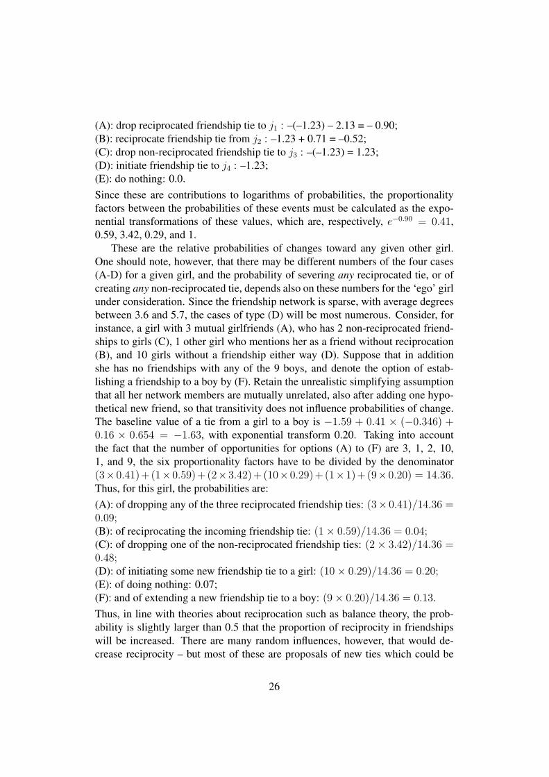
Transitivity and other triadic effectsNext to reciprocity, an essential feature in most social networks is the tendencytoward transitivity, or transitive closure (sometimes called clustering): friends offriends become friends, or in graph-theoretic terminology: two-paths tend to be,or to become, closed (e.g., Davis 1970, Holland and Leinhardt 1971). In Figure1.a, the two-path i→ j → h is closed by the tie i→ h.

Figure 1. a. Transitive triplet (i, j, h) b. Three-cycle

i

h

j

i

h

j

The transitive triplets effect measures transitivity for an actor i by counting thenumber of pairs j, h such that there is the transitive triplet structure of Figure 1.a.However, this is just one way of measuring transitivity. Another one is the transi-tive ties effect, which measures transitivity for actor i by counting the number ofother actors h for which there is at least one intermediary j forming a transitivetriplet of this kind. The transitive triplets effect postulates that more intermediarieswill add proportionately to the tendency to transitive closure, whereas the transi-tive ties effect expects that given that one intermediary exists, extra intermediarieswill not further contribute to the tendency to forming the tie i→ h.

An effect closely related to transitivity is balance (cf. Newcomb, 1962), whichin our implementation is the same as structural equivalence with respect to out-ties (cf. Burt, 1982), which is the tendency to have and create ties to other actorswho make the same choices as ego. The extent to which two actors make thesame choices can be expressed simply as the number of outgoing choices andnon-choices that they have in common.

Transitivity can be represented by still more effects: e.g., negatively, by thenumber of others to whom i is indirectly tied but not directly (geodesic distanceequal to 2). The choice between these representations of transitivity may depend

11

both on the degree to which the representation is theoretically convincing, and onwhat gives the best fit.

A different triadic effect is the number of three-cycles that actor i is involvedin (Figure 1.b). Davis (1970) found that in many social network data sets, there isa tendency to have relatively few three-cycles, which can be represented here bya negative parameter βk for the three-cycle effect. The transitive triplets and thethree-cycle effects both represent closed structures, but whereas the former is inline with a hierarchical ordering, the latter goes against such an ordering. If thenetwork has a strong hierarchical tendency, one expects a positive parameter fortransitivity and a negative for three-cycles. Note that a positive three-cycle effectcan also be interpreted, depending on the context of application, as a tendencytoward generalized exchange (Bearman, 1997).

Degree-related effectsIn- and outdegrees are primary characteristics of nodal position and can be impor-tant driving factors in the network dynamics.

One pair of effects is degree-related popularity based on indegree or outde-gree. If these effects are positive, nodes with higher indegree, or higher outdegree,are more attractive for others to send a tie to. This can be measured by the sumof indegrees of the targets of i’s outgoing ties, and the sum of their outdegrees,respectively. A positive indegree-related popularity effect implies that high inde-grees reinforce themselves, which will lead to a relatively high dispersion of theindegrees (a Matthew effect in popularity as measured by indegrees, cf. Merton,1968 and Price, 1976). A positive outdegree-related popularity effect will increasethe association between indegrees and outdegrees, or keep this association rela-tively high if it is high already.

Another pair of effects is degree-related activity for indegree or outdegree:when these effects are positive, nodes with higher indegree, or higher outdegreerespectively, will have an extra propensity to form ties to others. These effectscan be measured by the indegree of i times i’s outdegree; and, respectively, theoutdegree of i times i’s outdegree, that is, the square of the outdegree.1 Theoutdegree-related activity effect again is a self-reinforcing effect: when it has apositive parameter, the dispersion of outdegrees will tend to increase over time,or to be sustained if it already is high. The indegree-related activity effect has thesame consequence as the outdegree-related popularity effect: positive parameterslead to a relatively high association between indegrees and outdegrees. There-fore these two effects will be difficult, or impossible, to distinguish empirically,

1Experience has shown that for the degree-related effects, often the ‘driving force’ is measuredbetter by the square roots of the degrees than by raw degrees. In some cases this may be supportedby arguments about diminishing returns of increasingly high degrees. See the formulae in theappendix.

12

and the choice between them will have to be made on theoretical grounds. Thesefour degree-related effects can be regarded as the analogues in the case of directedrelations of what was called cumulative advantage by Price (1976) and preferen-tial attachment by Barabasi and Albert (1999) in their models for dynamics ofnon-directed networks: a self-reinforcing process of degree differentiation.

These degree-related effects can represent hierarchy between nodes in the net-work, but in a different way than the triadic effects of transitivity and 3-cycles.The degree-related effects represent global hierarchy while the triadic effects re-present local hierarchy. In a perfect hierarchy, ties go from the bottom to thetop, so that the bottom nodes have high outdegrees and low indegrees and the topnodes have low outdegrees and high indegrees. This will be reflected by positiveindegree popularity and negative outdegree popularity, and by positive outdegreeactivity and negative indegree activity. Therefore, to differentiate between localand global hierarchical processes, it can be interesting to estimate models withtriadic and degree-related effects, and assess which of these have the better fit bytesting the triadic parameters while controlling for the degree-related parameters,and vice versa.

Other degree-related effects are assortativity-related: actors might have pref-erences for other actors based on their own and the other’s degrees (Morris andKretzschmar 1995; Newman 2002). In settings where degrees reflect status ofthe actors, such preferences may be argued theoretically based on status-specificpreferences, constraints, or matching processes. This gives four possibilities, de-pending on in- and outdegree of the focal actor and the potential friend.

Together, this list offers eight degree-related effects. The outdegree-relatedpopularity and indegree-related activity effects are nearly collinear, and it was al-ready mentioned that theory, not empirical fit, will have to decide which one isa more meaningful representation. Some of the other effects also may be con-founded, but this depends on the data set. The four effects described as degree-related popularity and activity are more basic than the assortativity effects (cf. therelation between main effects and interactions in linear regression). Because ofthis, when testing any assortativity effects, one usually should control for three ofthe degree-related popularity and activity effects.

Covariates: exogenous effectsFor an actor variable V , there are three basic effects: the ego effect, measuringwhether actors with higher V values tend to nominate more friends and hencehave a higher outdegree (which also can be called covariate-related activity ef-fect or sender effect); the alter effect, measuring whether actors with higher Vvalues will tend to be nominated by more others and hence have higher indegrees(covariate-related popularity effect, receiver effect); and the similarity effect, mea-suring whether ties tend to occur more often between actors with similar values on

13

V (homophily effect). Tendencies to homophily constitute a fundamental charac-teristic of many social relations, see McPherson, Smith-Lovin, and Cook (2001).When the ego and alter effects are included, instead of the similarity effect onecould use the ego-alter interaction effect, which expresses that actors with higherV values have a greater preference for other actors who likewise have higher Vvalues.

For categorical actor variables, the same V effect measures the tendency tohave ties between actors with exactly the same value of V .

For a dyadic covariate, i.e., a variable defined for pairs of actors, there is onebasic effect, expressing the extent to which a tie between two actors is more likelywhen the dyadic covariate is larger.

InteractionsLike in other statistical models, interactions can be important to express theo-retically interesting hypotheses. The diversity of functions that could be used aseffects makes it difficult to give general expressions for interactions. The ego-alterinteraction effect for an actor covariate, mentioned above, is one example.

Another example is given by de Federico (2004) as an interaction of a covari-ate with reciprocity. In her analysis of a friendship network between exchange stu-dents, she found a negative interaction between reciprocity and having the samenationality. Having the same nationality has a positive main effect, reflecting thatit is easier to become friends with those coming from the same country. The nega-tive interaction effect was unexpected, but can be explained by regarding recipro-cation as a response to an initially unreciprocated tie, the latter being a unilateralinvitation to friendship. Since contacts between those with the same national-ity are easier than between individuals from different nationalities, extending aunilateral invitation to friendship is more remarkable (and perhaps more costly)between individuals of different nationalities than between those of the same na-tionality. Therefore it will be noticed and appreciated, and hence reciprocated,with a higher probability. Thus, the rarity of cross-national friendships leads to astronger tendency to reciprocation in cross-national than same-nationality friend-ships.

As a further class of examples, note that in the actor-based framework it maybe natural to hypothesize that the strength of certain effects depends on attributesof the focal actor. For example, girls might have a greater tendency toward transi-tive closure than boys. This can be modeled by the interaction of the ego effect ofthe attribute and the transitive triplets, or transitive ties effect.

Other interactions (and still other effects) are discussed in Snijders et al. (2008).As the selection presented here already illustrates, the portfolio of possible effectsin this modeling approach is very extensive, naturally reflecting the multitude ofpossibilities by which networks can evolve over time. Therefore, the selection

14

of meaningful effects for the analysis of any given data set is vital. This will bediscussed now.

3. Issues arising in statistical modeling

When employing these models, important practical issues are the question how tospecify the model – boiling down mainly to the choice of the terms in the objectivefunction – and how to interpret the results. This is treated in the current section.

3.1. Data requirements

To apply this model, the assumptions should be plausible in an approximate sense,and the data should contain enough information. Although rules of thumb alwaysmust be taken with many grains of salt, we first give some numbers to indicate thesizes of data sets which might be well treated by this model. These rules of thumbare based on practical experience.

The amount of information depends on the number of actors, the number ofobservation moments (‘panel waves’), and the total number of changes betweenconsecutive observations. The number of observation moments should be at least2, and is usually much less than 10. There are no objections in principle againstanalyzing a larger number of time points, but then one should check the assump-tion that the parameters in the objective function are constant over time, or thatthe trends in these parameters are well represented by their interactions with timevariables (see point 10 below).

If one has more than two observation points, then in practice one may wish tostart by analyzing the transitions between each consecutive pair of observations(provided these provide enough information for good estimation – see below). Foreach parameter one then can present the trend in estimated parameter values, anddepending on this one can make an analysis of a larger stretch of observations ifthe parameters appear approximately constant, or do the same while including forsome of the parameters an interaction with a time variable.

The number of actors will usually be larger than 20 – but if the data containmany waves, a smaller number of actors could be acceptable. The number of ac-tors will usually not be more than a few hundred, because the implicit assumptionthat each actor is a potential network partner for any other actor might be implau-sible for networks with so many actors that not all actors are aware of each others’existence.

The total number of changes between consecutive observations should be largeenough, because these changes provide the information for estimating the param-eters. A total of 40 changes (cumulated over all successive panel waves) is on

15

the low side. More changes will give more information and, thereby, allow morecomplicated models to be fitted. Between any pair of consecutive waves, the num-ber of changes should not be too high, because this would call into question theassumption that the waves are consecutive observations of a gradually changingnetwork; or, if they were, the consecutive observations would be too far apart.

This implies that, when designing the study, the researcher has to have a rea-sonable estimate of how much change to expect. For instance, if one is inter-ested in the development of the friendship network of a group of initially mutualstrangers (e.g., university freshmen), it may be good to plan the observation mo-ments to be separated by only a few weeks, and to enlarge the period betweenobservations after a couple of months. On the other hand, if one studies inter-firmnetwork dynamics, given the time delays involved for firms in the planning andexecuting of their ties to other firms, it may be enough to collect data once everyyear, or even less frequently.

To express quantitatively whether the data collection points are not too farapart, one may use the Jaccard (1900) index (also see Batagelj and Bren, 1995),applied to tie variables. This measures the amount of change between two wavesby

N11

N11 +N01 +N10

, (2)

where N11 is the number of ties present at both waves, N01 is the number of tiesnewly created, and N10 is the number of ties terminated. Experience has shownthat Jaccard values between consecutive waves should preferably be higher than.3, and – unless the first wave has a much lower density than the second – valuesless than .2 would lead to doubts about the assumption that the change process isgradual, compared to the observation frequency. If the network is in a period ofgrowth and the second network has many more ties than the first, one may lookinstead at the proportion, among the ties present at a given observation, of tiesthat have remained in existence at the next observation (N11/(N10 + N11) in thepreceding notation). Proportions higher than .6 are preferable, between .3 and .6would be low but may still be acceptable. If the data collection was such thatvalues of ties (ranging from weak to strong) were collected, then these numbersmay be used as rough rules of thumb and give some guidance for the decisionwhere to dichotomize the tie values – although, of course, substantive concernsrelated to the interpretation of the results have primacy for such decisions.

The methods require in principle that network data are complete. However, itis allowed that some of the actors enter the network after the start, or leave beforethe end of the panel waves (Huisman and Snijders, 2003), and a limited amountof missing data can be accommodated (Huisman and Steglich, 2008). Anotheroption to represent that some actors are not yet, or no more, present in the net-

16

work, is to specify that certain ties cannot exist (‘structural zeros’) or that someties are prescribed (‘structural ones’), see Snijders et al. (2008). The use of struc-tural zeros allows, e.g., to combine several small networks into one structure (withstructural zeros forbidding ties between different networks), allowing to analyzemultiple independent networks that on themselves would not yield enough in-formation for estimating parameters, under the extra assumption that all networkfollow dynamics with the same parameter values in the objective function.

3.2. Testing and model selection

It turns out (supported by computer simulations) that the distributions of the esti-mates of the parameters βk in the objective function (1), representing the impor-tance of the various terms mentioned in Section 2.3, are approximately normallydistributed. Therefore these parameters can be tested by referring the t-ratio, de-fined as parameter estimate divided by standard error, to a standard normal distri-bution.

For actor-based models for network dynamics, information-theoretic modelselection criteria have not yet generally been developed, although Koskinen (2004)presents some first steps for such an approach. Currently the best possibility isto use ad hoc stepwise procedures, combining forward steps (where effects areadded to the model) with backward steps (where effects are deleted). The stepscan be based on significance test for the various effects that may be included in themodel. Guidelines for such procedures are the following. We prefer not to givea recipe, but rather a list of considerations that a researcher might have in mindwhen constructing a strategy for model selection.

1. Like in all statistical models, exclusion of one effect may mask the existenceof another effect, so that pure forward selection may lead to overlookingsome effects, and it is advisable to start with a model including all effectsthat are expected to be strong.

2. Fitting complicated models may be time-consuming and lead to instabilityof the algorithm, and a resulting failure to obtain good estimates. Therefore,forward selection is technically easier than backward selection, which isunfortunately at variance with the preceding remark.

3. The estimation algorithm (Snijders, 2001) is iterative, and the initial valuecan determine whether or not the algorithm converges. For relatively simplemodels, a simple standard initial value usually works fine. For complicatedmodels, however, the algorithm may converge more easily if started froman initial value obtained as the estimate for a somewhat simpler model. Es-timates obtained from a more complicated model by simply omitting the

17

deleted effects sometimes do not provide good starting values. Therefore,forward selection steps often work better from the algorithmic point of viewthan backward steps. This implies that, to improve the performance of thealgorithm, it is advisable to retain copies of the parameter values obtainedfrom good model fits, for use as possible initial values later on.

4. Network statistics can be highly correlated just because of their definition.This also implies that parameter estimates can be rather strongly correlated,and high parameter correlations do not necessarily imply that some of theeffects should be dropped. For example, the parameter for the outdegreeeffect often is highly correlated with various other structural parameters.This correlation tells us that there is a trade-off between these parametersand will lead to increased standard errors of the parameter for the outdegreeeffect, but it is not a reason for dropping this effect from the model.

5. Parameters can be tested by a so-called score-type test without estimatingthem, as explained in Schweinberger (2008). Since estimating many pa-rameters can make the algorithm instable, and in forward selection steps itmay be necessary to have tests available for several effects to choose themost important one to include, the score-type tests can be very helpful inmodel selection. In this procedure, a model (null hypothesis) including sig-nificant and/or theoretically relevant parameters is tested against a model(alternative hypothesis) extended by one or several parameters one is alsointerested in. Under the null hypothesis, those parameters are zero. Theprocedure yields a test statistic with a chi-squared null distribution, alongwith standard normal test statistics for each separate parameter. The param-eters for which a significant test result was found, then may be added to themodel for a next estimation round.

6. It is important to let the model selection be guided by theory, subject-matterknowledge, and common sense. Often, however, theory and prior know-ledge are stronger with respect to effects of covariates – e.g., homophilyeffects – than with respect to structure. Since a satisfactory fit is importantfor obtaining generalizable results, the structural side of model selectionwill of necessity often be more of an inductive nature than the selection ofcovariate effects. The newness of this method implies that we still needto accumulate more experience as to what is a ‘satisfactory’ fit, and howcomplicated models should be in practice.

7. Among the structural effects, the outdegree and reciprocity effect should beincluded by default. In almost all longitudinal social network data sets, therealso is an important tendency toward transitivity (Davis 1970). This should

18

be modeled by one, or several, of the transitivity-related effects describedabove.

8. Often, there are some covariate effects which are predicted by theory; thesemay be control effects or effects occurring in hypotheses. It is good prac-tice to include control effects from the start. Non-significant control effectsmight be dropped provisionally and then tested again as a check in the pre-sumed final model; but one might also retain control effects independent oftheir statistical significance. We do not think there are unequivocal ruleswhether or not to include from the start the effects representing the mainhypotheses in a given study.

9. The degree-based effects (popularity, activity, assortativity) can be impor-tant structural alternatives for actor covariate effects, and can be importantnetwork-level alternatives for the triad-level effects. It is advisable, at somemoment during the model selection process, to check these effects; note thatthe square-root specification usually works best.

10. If the data have three or more waves and the model does not include time-changing variables, then the assumption is made that the time dynamics ishomogeneous, which will lead to smooth trajectories of the main statisticsfrom wave to wave. It is good as a first general check to consider how aver-age degree develops over the waves, and if this development does not followa rather smooth curve (allowing for random disturbances), to include time-varying variables that can represent this development. Another possibilityis to analyze consecutive pairs of waves first, which will show the extent ofinhomogeneity in the process (cf. the example in Snijders, 2005).

11. The model assumes that the ‘rules for network change’ are the same forall actors, except for differences implied by covariates or network position.This leaves only moderate room for outlying actors, such as are indicatedby relatively very large outdegrees or indegrees. Very high or very lowoutdegrees or indegrees should be ‘explainable’ from the model specifica-tion; if they are only explainable from earlier observations (‘path depen-dence’), they will have a tendency to regress toward the mean. The modelspecification may be able to explain outliers by covariates identifying ex-ceptional actors, but also by degree-related endogenous effects such as theself-reinforcing Matthew effect mentioned above. It is good as a first gen-eral check to inspect the indegrees and outdegrees for outliers. If there arestrong outliers then it is advisable to seek for actor covariates which can helpto explain the outlying values, or to investigate the possibility that degree-related effects, explainable or at least interpretable from a theoretical point

19

of view, may be able to represent these outlying degrees. If these cannotbe found, then one solution is to use dummy variables for the actors con-cerned, to represent their outlying behavior. Such an ad hoc model adapta-tion, which may improve the fit dramatically, is better than the alternative ofworking with a model with a large unmodeled heterogeneity. In case thereis a theoretical argument to expect certain outliers, these can be pointed outby including a dummy variable, but of a different kind. In contrast to theformer type of outliers, the latter one is expected, so should be captured inadvance by a covariate. If one is not capable to make a difference betweenthe two types, one has to rely on the ad hoc model adaptation.

3.3. Example: friendship dynamics

By way of example, we analyze the evolution of a friendship network in a Dutchschool class. The data were collected between September 2003 and June 2004 aspart of a study reported in Knecht (2008). The 26 students were followed overtheir first year at secondary school during which friendship networks as well asother data were assessed at four time points at intervals of three months. Therewere 17 girls and 9 boys in the class, aged 11-13 at the beginning of the schoolyear. Network data were assessed by asking students to indicate up to twelveclassmates which they considered good friends. The average number of nomi-nated classmates ranged between 3.6 and 5.7 over the four waves, showing a mod-erate increase over time. Jaccard coefficients for similarity of ties between wavesare between .4 and .5, which is somewhat low (reflecting fairly high turnover) butnot too low.

Some data were missing due to absence of pupils at the moment of data col-lection. This was treated by ad-hoc model-based imputation using the procedureexplained in Huisman and Steglich (2008). One pupil left the classroom. Suchchanges in network composition can also be treated by the methods of Huismanand Snijders (2003), but this simple case was treated here by using structural ze-ros: starting with the first observation moment where this pupil was not a memberof the classroom any more, all incoming and outgoing tie variables of this pupilwere fixed to zero and not allowed to change in the simulations.

Considering point 1 above, effects known to play a role in friendship dynam-ics, such as basic structural effects and effects of basic covariates, are included inthe baseline model. From earlier research, it is known that friendship formationtends to be reciprocal, shows tendencies towards network closure, and in this agegroup is strongly segregated according to the sexes. The model includes, for eachof these tendencies, effects corresponding to these expectations. Structural effectsincluded are reciprocity; transitive triplets and transitive ties, measuring transitiveclosure that is compatible with an informal local hierarchy in the friendship net-

20

work; and the three-cycles effect measuring anti-hierarchical closure. Homophilybased on the sexes is included as the same sex effect. All variables are centered.For example, the dummy variable for sex (boys = 1, girls = 0) has mean 0.346 (9boys and 17 girls), which leads to the centered values vi = –0.346 for girls and vi

= 0.654 for boys.As exogenous control variables, we include sender and receiver effects of sex,

and a dyadic covariate indicating friendship in primary school reflecting relation-ship history. In addition, several degree-related endogenous effects are includedas control effects: in- and outdegree-related popularity, and outdegree-related ac-tivity, explained above. Estimates for this model are given in Table 1 as Model 0.All calculations were done using Siena version 3.2 (Snijders et al., 2008).

The parameters reported for the rate function in periods 1-3 are defined in thesimulation model as the expected frequencies, between successive waves, withwhich actors get the opportunity to change a network tie. For these parameters nop-values are given in the tables, as testing that they are zero is meaningless (if thesewould be zero there would be no change at all). These estimated rate parameterswill be higher than the observed numbers of changes per actor, however, becausein the model an actor may get the opportunity to change a tie but choose not tomake any change, and because actors may add a tie during the simulations, andwithdraw the same tie before the next observation moment.

Table 1 about hereThis analysis confirms, for this data set, several of the known properties of

friendship networks: there is a high degree of reciprocity, as seen in the signif-icant reciprocity parameter; there is segregation according to the sexes, as seenin the significant same sex parameter; there is an almost equally strong effect ofhaving been friends at primary school already, and there is evidence for transitiveclosure, as seen in the significant effects of transitive triplets and transitive ties.A direct comparison of the size of parameter estimates is possible, given that theyoccur in the same linear combination in the objective function, but it should bekept in mind that these are unstandardized coefficients. Other significant effectsare the negative 3-cycles parameter, which indicates that the tendencies towardclosure are not completely egalitarian (as one might have thought based on thereciprocity parameter), but do show some evidence for local hierarchization inthe network. This also is suggested by the marginally significant negative effectof the outdegree-related popularity which indicates that active pupils, i.e., thosewho nominate particularly many friends, are less likely to be chosen as friends –this could be a status effect negatively associated with nomination activity. Alsosignificant is the sender effect of sex (sex (M) ego), which in our coding of thevariable means that the boys tend to be more active in the classroom friendshipnetwork than the girls.

21

Rate parameters, finally, suggest that the amount of friendship change seemsto peak in the second period (perhaps due to a higher friendship turnover afterthe Christmas break) and slow down towards the end of the school year. Thesedifferences are small, however. The same descriptive conclusion can be drawnalso by inspecting the observed amounts of change, without needing to refer to astatistical model.

In a subsequent model (Model 1 in Table 1), more parsimony is obtained byeliminating the non-significant effects in a backward selection procedure. The sexalter effect was retained in spite of its non-significance, because the three sex-related effects belong together as a representation of sex-related friendship pref-erences. One by one, the least significant of the insignificant effects were droppedfrom the model. While doing so, score-type tests were made for the earlier omit-ted parameters (now constrained to zero) to check whether the parameter does notbecome significant upon dropping other effects from the model. This is possi-ble in models with correlated effects like ours, but it did not occur for our dataset. Estimates of Model 1 give the same qualitative results as those of Model 0.The parameters dropped due to insignificance were the outdegree-related activityeffect (suggesting that the value for ego of an individual friendship does not de-pend on how many other friends the friend currently has) and the indegree-relatedpopularity effect (suggesting that receiving many friendship nominations is not aself-reinforcing process).

3.4. Parameter interpretation

For the general understanding of the numerical values of the parameters, it may bekept in mind that the parameters βk in the objective function are unstandardizedcoefficients of the statistics of which the mathematical formulae are given in theappendix.

The parameters in the objective function can be interpreted in two ways. Inthe first place, by interpreting this function as the “attractiveness” of the networkfor a given actor. For getting a feeling of what are small and large values, it maybe noted (see the interpretation in terms of myopic optimization in Snijders, 2001)that the objective functions are used to compare how attractive various differenttie changes are, and for this purpose random disturbances are added to the valuesof the objective function with standard deviations equal2 to 1.28.

The objective function is a weighted sum of effects sik(x); their mathematicaldefinitions are given in the appendix. In most cases the contribution of a single tievariable xij is just a simple component of this formula.

For example, consider the actor variable sex, denoted as V , and originally

2More exactly, the value is√π2/6, the standard deviation of the Gumbel distribution.

22

with values 1 for girls and 2 for boys. All variables are centered. The globalmean of this variable is 1.346 (9 boys and 17 girls), which leads to the centeredvalues vi = −0.346 for girls and vi = 0.654 for boys. For this variable the modelincludes the ‘ego’ effect, the ‘alter’ effect, and the ‘same’ effect. Let us denote theparameters by βe, βa, and βs. Then, using the formulae in the appendix, the jointcontribution of these V -related effects to the objective function is

βe

∑j

xij vi + βa

∑j

xij vj + βs

∑j

xij I{vi = vj}

where I{vi = vj} = 1 if vi = vj , and 0 otherwise. This means that the contribu-tion of the single tie xij to the objective function, considering only the sex-relatedeffects, is given by

βe vi + βa vj + βs I{vi = vj} = 0.35 vi + 0.10vj + 0.49 I{vi = vj}

Substituting the values -0.346 for females and 0.654 for males yields the followingtable.

alterego F M

F 0.33 –0.06M 0.19 0.78

This table shows that girls as well as boys prefer friendships with same-sexalters, but for boys the difference is more pronounced than for girls.

A second interpretation is that when actor i has the opportunity to make achange in her outgoing ties (where no change also is an option), and xa and xb aretwo possible results of this change, then fi(xb, β)− fi(xa, β) is the log odds ratiofor choosing between these two alternatives – so that the ratio of the probabilityof xb and xa as next states is

exp(fi(xb, β)− fi(xa, β)

)=

exp(fi(xb, β)

)exp

(fi(xa, β)

) .Note that, when the current state is x, the possibilities for xa and xb are x itself (nochange), or x with one extra outgoing tie from i, or x with one less outgoing tiefrom i. Explanations about log odds ratios can be found in texts about logistic re-gression and loglinear models, e.g., Agresti (2002). A further elaborated exampleof this is given below in Section 4.2.

23

4. More complicated models

This section treats two generalizations of the model sketched above.

4.1. Differential rates of change: the rate function

Depending on actor attributes or on positional characteristics such as indegree oroutdegree, actors might change their ties at differential frequencies. This can bethe case, e.g., in networks between organizations with clear differences in degrees,where the outdegrees reflect the importance to the organizations of the networkunder study, and the resources they devote to positioning themselves in it. Theaverage frequency at which actors get the opportunity to change their outgoingties then is called the rate function, depending on attributes and network positionof the actors.

Model 2 in Table 1 gives an example of such an analysis. It extends Model 1 byadding an effect of sex on the rate function. The estimated negative effect indicatesthat in the data set under study, boys change their network ties less frequently thangirls, but the difference is not significant (p = 0.13).

To interpret the parameter values, one should know that a so-called exponen-tial link function is used (Snijders, 2001; Snijders et al., 2008), which means thatthe variables have an effect on the rate function after an exponential transforma-tion, with a multiplicative effect. For example, the parameter estimate of –0.42 forthe effect of sex on the rate function implies that the estimated rate function is thebase rate multiplied by exp(−0.42 vi). Recall that the values of the variable ‘sex’are, centered, vi = −0.346 for females and vi = 0.654 for males. Thus, for period1, for girls the expected number of opportunities for change is 9.69×exp(−0.42×(−0.346)) = 11.2, and for boys it is 9.69 × exp(−0.42 × (0.654)) = 7.4. Thedifference seems rather large but is not significant in view of the small samplesize.

4.2. Differences between creating and terminating ties: the endowment function

In the treatment given above, terminating a tie is just the opposite of creatingone. This is not always a good representation of reality. It is conceivable, forexample, that the loss when terminating a reciprocal tie is greater than the gainin creating one; or that transitive closure works especially for the creation of newties, but hardly guards against termination of existing ties. This can be modeled byhaving two components of the objective function: the evaluation function, whichconsiders only the network that will be the case as a result of the change to bemade; and the endowment function, which is a component that operates only forthe termination of ties and not for their creation. Everything discussed above about

24

the objective function concerned the evaluation function – in other words, in thosediscussions and the example, the endowment function was nil. The endowmentfunction gives contributions to the objective function that do not play a role whencreating ties, but that are lost when dissolving ties.

Model 3 in Table 1 gives the results of an analysis that includes, in addi-tion to the effects of Model 1, also an endowment effect related to reciprocity.It was estimated as significant and positive, while the corresponding evaluationfunction effect of reciprocity dropped in size and significance. To interpret thisresult, jointly consider the reciprocity evaluation effect with parameter 0.71 andthe reciprocity endowment effect with parameter 1.42. The contribution of a tiebeing reciprocated then is 0.71 for the creation of the tie and 0.71 + 1.42 = 2.13against the termination of the tie. Thus, reciprocity here is more important againstterminating friendships – that is, for maintaining friendships – than for creatingfriendships.

To elaborate this example, consider how the friendship choices of a girl to-wards other girls depend on reciprocity. Suppose that actor i can change one ofher ties, while there are two girls j1 and j2, both of them choosing i as a friend,and two others j3 and j4 not choosing i. In addition, suppose that currently ichooses j1 and j3 as friends, but not the other two. Assume finally (artificially, forthe sake of explanation) that these four girls do not choose each other and furtheralso are isolated from i’s network so that other structural effects besides recipro-city do not matter. Since the actor variable ‘sex’ has centered value vi = −0.346for girls, the parameter estimates for Model 3 give as the total contribution of thethree sex-related effects for girl-girl ties 0.41 vi + 0.16 vj + 0.56 I{vi = vj} =(0.41 + 0.16)× (−0.346) + 0.56 = 0.36. With the outdegree effect of –1.59, thisyields −1.59 + 0.36 = −1.23 as the basic contribution of a tie to the evaluationfunction.

Option A: drop tie? Option B: add tie?

Option C: drop tie? Option D: add tie?

ego

i

j1 j2

j3 j4

Figure 2. Four options for actor i.

When girl i can change a tie variable, using this value of –1.23 for the combinedeffect of outdegree and the three sex-related effects for a girl-girl tie, five of theoptions for i are the following:

25

(A): drop reciprocated friendship tie to j1 : –(–1.23) – 2.13 = – 0.90;(B): reciprocate friendship tie from j2 : –1.23 + 0.71 = –0.52;(C): drop non-reciprocated friendship tie to j3 : –(–1.23) = 1.23;(D): initiate friendship tie to j4 : –1.23;(E): do nothing: 0.0.Since these are contributions to logarithms of probabilities, the proportionalityfactors between the probabilities of these events must be calculated as the expo-nential transformations of these values, which are, respectively, e−0.90 = 0.41,0.59, 3.42, 0.29, and 1.

These are the relative probabilities of changes toward any given other girl.One should note, however, that there may be different numbers of the four cases(A-D) for a given girl, and the probability of severing any reciprocated tie, or ofcreating any non-reciprocated tie, depends also on these numbers for the ‘ego’ girlunder consideration. Since the friendship network is sparse, with average degreesbetween 3.6 and 5.7, the cases of type (D) will be most numerous. Consider, forinstance, a girl with 3 mutual girlfriends (A), who has 2 non-reciprocated friend-ships to girls (C), 1 other girl who mentions her as a friend without reciprocation(B), and 10 girls without a friendship either way (D). Suppose that in additionshe has no friendships with any of the 9 boys, and denote the option of estab-lishing a friendship to a boy by (F). Retain the unrealistic simplifying assumptionthat all her network members are mutually unrelated, also after adding one hypo-thetical new friend, so that transitivity does not influence probabilities of change.The baseline value of a tie from a girl to a boy is −1.59 + 0.41 × (−0.346) +0.16 × 0.654 = −1.63, with exponential transform 0.20. Taking into accountthe fact that the number of opportunities for options (A) to (F) are 3, 1, 2, 10,1, and 9, the six proportionality factors have to be divided by the denominator(3×0.41) + (1×0.59) + (2×3.42) + (10×0.29) + (1×1) + (9×0.20) = 14.36.Thus, for this girl, the probabilities are:(A): of dropping any of the three reciprocated friendship ties: (3× 0.41)/14.36 =0.09;(B): of reciprocating the incoming friendship tie: (1× 0.59)/14.36 = 0.04;(C): of dropping one of the non-reciprocated friendship ties: (2× 3.42)/14.36 =0.48;(D): of initiating some new friendship tie to a girl: (10× 0.29)/14.36 = 0.20;(E): of doing nothing: 0.07;(F): and of extending a new friendship tie to a boy: (9× 0.20)/14.36 = 0.13.Thus, in line with theories about reciprocation such as balance theory, the prob-ability is slightly larger than 0.5 that the proportion of reciprocity in friendshipswill be increased. There are many random influences, however, that would de-crease reciprocity – but most of these are proposals of new ties which could be

26

seen by the other party as an invitation toward future reciprocation.

5. Dynamics of networks and behavior

Social networks are so important also because they are relevant for behavior andother actor-level outcomes: related actors may influence one another (e.g., Fried-kin, 1998), and ties will be selected in part based on the similarity between ego andpotential relational partners (homophily, see McPherson, Smith-Lovin, and Cook,2001). This means that not only is the network changing as a function of itself andof the actor variables, but likewise the actor variables are changing as a functionof themselves and of the network. We use the term behavior as shorthand for en-dogenously changing actor variables, although these could also refer to attitudes,performance, etc.; there could be one or more of such variables. It is assumed herethat the behavior variables are ordinal discrete variables, with values 1, 2, etc., upto some maximum value, for instance, several levels of delinquency, several levelsof smoking, etc. The dependence of the network dynamics on the total network-behavior configuration will be also called the social selection process, while thedependence of the behavior dynamics on the total network-behavior configura-tion will be called the social influence process. Both social influence and socialselection can lead to similarity between tied actors, which is often observed. Afundamental question then is whether this similarity is caused mainly by influenceor mainly by selection, as discussed by Ennett and Bauman (1994) for smokingbehavior and Haynie (2001) for delinquent behavior.

This combination of selection and influence can be modeled by an extensionof the actor-based model to a structure where the dependent variables consist notonly of the tie variables but also of the actors’ behavior variables, as specified inSnijders, Steglich and Schweinberger (2007) and Steglich, Snijders and Pearson(2009). Of course there usually will be, in addition, also exogenous actor and/ordyadic variables in the role of independent variables.

The assumptions for the actor-based model for the dynamics of networks andbehavior are extensions of the assumptions for network dynamics. The extendedformulations are as follows, given without the background explanations whichwere given above and which apply also for this case.

1. As above, the underlying time parameter is continuous.

2. The changing system consisting of network and behavior is the outcome ofa Markov process. Thus, the probabilities of change of the network as wellas those of the behavioral variables depend, at each moment, on the currentcombination of network structure and behavior variables for all actors.

27

3. At a given moment either one probabilistically selected actor may change atie, or one actor may change his/her behavior by going one unit up or down(recall that the behavior variables are assumed to be integer-valued). Thisexcludes coordination between changes in the network and in the behavior.

The fact that changes in behavior are assumed to be by one unit in a singletime point imply that a ‘natural’ application of the model requires that thetotal number of ordinal scale values is not too large; in practice applicationsmostly have had two to five, and sometimes up to ten, scale values.

4. The actors control their outgoing ties as well as their own behavior. Thisis meant not in the sense of conscious control, but in the sense that theexplanation of the actor’s outgoing ties and behavior is based in the actorand the structural and other limitations provided by the actor and his/hersocial context.

5. The moments were actors get the opportunity for a tie change or a behaviorchange are modeled as distinct processes, so these are governed by a prioriunrelated parameters.

6. There are distinct processes also for tie changes and behavior changes, con-ditional on the possibility to make the respective type of change, so theseare governed by a priori unrelated parameters.

The changes in behavior depend on an objective function similar to the objectivefunction for network changes. However, this function will be different becauseit needs to represent primarily the actor’s behavior rather than his/her networkposition, and because choices of behavior changes may be framed differently fromchoices of tie changes, depending on different goals and restrictions.

The model assumptions imply that the dependent behavior variable will changeendogenously during the simulations, representing the endogenous social influ-ence process. Since the network and the behavior variables both influence thedynamics of the network ties and of the actors’ behavior, the sequence of changesin the network and in the behavior, reacting on each other, generates a mutualdependence between the network dynamics and the behavior dynamics.

5.1. The objective function for behavior

We only consider models where increasing the behavior variable has just the op-posite effect of decreasing it, and the objective function for behavior is the sameas the evaluation function (a separate endowment function is not considered). The

28

objective, or evaluation, function can be represented, analogously to (1), as

fZi (β, x, z) =

∑k

βZk s

Zki(x, z) , (3)

where sZki(x, z) are functions depending on the behavior of the focal actor i, but

also on the behavior of his network partners, his network position, etc. Thestrength of the effects of these functions on behavior choices are represented bythe parameters βZ

k . The superscript Z is used to distinguish the effects and param-eters for behavior change from those for network change (which could be giventhe superscript X). The main possible terms of the evaluation function are asfollows.

Basic shape effectsWe first discuss basic tendencies determining behavior change that are indepen-dent of actor attributes and network position. A baseline definition for the eval-uation function will be a curve, depending on the actor’s own behavior zi, thatcan be loosely interpreted as the relative preference for the specific value zi of thebehavior. The term ‘prefer’ should be taken with much reservation, as a shorthand‘as-if’ term – we could just as well see this, e.g., as a matter of constraints. Whenthe behavior variable is dichotomous, then a linear function suffices, as each func-tion of two values can be represented by a linear function; but for three or morepossible values a unimodal ‘preference’ function will often be reasonable, so thata specification will be required that allows the function to be curvilinear. Thus,in Figure 3, a simple evaluation function is drawn for a behavior variable withrange 1–4, which is maximal at the value z = 2, indicating that when actors havea possibility for change they will be drawn toward the value z = 2: if their currentvalue for Z is higher than 2 then the probability is higher that they will decreasetheir value, if the current value is lower than 2 then the probability is higher thatthey will increase their value of Z. To represent this mathematically, a quadraticfunction can be used. The linear and quadratic coefficients in this function arecalled the linear shape effect and the quadratic shape effect. Note that the latter issuperfluous for a dichotomous behavior variable.

29

z

fZi (β, x, z)

1 2 3 4

Figure 3. Basic shape of the evaluation function for behavior;in this case, with the maximum at z = 2.

The quadratic shape effect can also be called the effect of Z on itself, andis a kind of feedback effect. When this parameter is negative there is negativefeedback, or a self-correcting mechanism: when the value of the actor’s behav-ior increases, the further push toward higher values of the behavior will becomesmaller and when it decreases, the further push toward lower values of the behav-ior will become smaller. Conversely, when the coefficient of the quadratic termis positive, the feedback will be positive, so that changes in the behavior are self-reinforcing. This can be an indication of addictive behavior. Negative values, orvalues not significantly different from 0, are more often seen than positive values.

When the coefficient for the shape effect is denoted βZ1 and the coefficient for

the quadratic shape effect is βZ2 , then the total contribution of these two effects

is βZ1 zi + βZ

2 z2i . With a negative coefficient βZ

2 , this is a unimodal preferencefunction. The maximum then is attained for zi = −2 βZ

1 /βZ2 , or more precisely,

the integer value within the prescribed range that is closest to this number. (Ofcourse additional effects will lead to a different picture; but if the additional effectsare linear as a function of zi in the permitted range – which can be checked fromthe formulae in the appendix, and which is not the case for all similarity effectsas defined below! –, this will change the location of the maximum but not theunimodal shape of the function.)

Influence and position-dependent effectsThe tendencies expressed in the shape parameters affect every actor in the sameway, irrespective of his/her characteristics or network position. To capture socialnetwork effects, additional terms in the behavior evaluation function are needed,differentiating between actors on the basis of their network position and the be-havior of the others to whom they are tied.

The actor-based model can represent social influence, i.e., influence from al-ters’ behavior on ego’s behavior, in various ways, because there are several dif-ferent ways to measure and aggregate the influences from different alters. Threedifferent representations are as follows.

30

1. The average similarity effect, expressing the preference of actors to be sim-ilar in behavior to their alters, in such a way that the total influence of thealters is the same regardless of the number of alters (i.e., ego’s outdegree).

2. The total similarity effect, expressing the preference of actors to be similarin behavior to their alters, in such a way that the total influence of the altersis proportional to the number of alters.

3. The average alter effect, expressing that actors whose alters have a higheraverage value of the behavior, also have themselves a stronger tendencytoward high values on the behavior.

The choice between these three will be made on theoretical grounds and/or on thebasis of statistical significance.

In addition to this type of social influence, network position itself could alsohave an effect on the dynamics of the behavior. Indeed, the actor’s outdegree orindegree may be terms in the objective function; in the case of positive param-eters, this expresses that those who are more active (higher outdegree) or morepopular (higher indegree) have a stronger tendency to display higher values of thebehavior.

Effects of other actor variablesFor each actor-dependent covariate as well as for each of the other dependentbehavior variables (if any), a main effect on the behavior can be included, repre-senting the influence of this actor variable on changes in the behavior. In addition,it is possible that such a variable will moderate the influence effect, leading to aninteraction between the variable and the influence effect.

5.2. Specification of models for dynamics of networks and behavior

There is a natural advantage of the network part of the model over the behaviorpart in terms of the amount of information available on the two dimensions. For nactors, there are nmeasurements of the behavior variable, while there are as manyas n(n− 1) measurements of network tie variables. In statistical terms, there willbe less power to detect determinants of behavioral evolution than there is to detectdeterminants of network evolution. Therefore, backward model selection is nota good route to follow for specifying a model of network-behavior co-evolution:weak and unsystematic effects on behavioral change, when estimated, subtractfrom the ability to identify the stronger and more systematically occurring ones.Instead of starting with an extensive model, it is better to start with a small one,and proceed by way of forward model selection to arrive at a good model.

31

Since it is more difficult to estimate a model of network-behavior co-evolutionthan to estimate a model of only network evolution, it makes sense first to estimatea good model for the dynamics of only the network according to the approach ofthe preceding section, and to use this as a baseline for the network part of theco-evolution model.

It has become clear above that there are several specifications of the socialselection part, such as Z-similarity and Z - ego × alter; like for any actor vari-able, also for behavior variable Z the ego and alter effects may be relevant. Thesimilarity effect in the network dynamics part is directly interpretable, whereasthe Z - ego × alter interaction effect needs also the ego and alter effects to bewell interpretable. For the social influence part likewise there are several possiblespecifications, such as average similarity, total similarity, and average alter.

A difficulty is that we often have no clear theoretical clue as to which of thesethree specifications is better in a particular case; the alternative specifications aredefined by effects that may be highly mutually correlated and therefore are notreadily estimated jointly in the same model; and the power of detecting selectionand influence will depend on the specification chosen. If we do have prior infor-mation as to the best specification, then it is preferable to work with this spec-ification. If we do not have such information, and we wish to avoid the chancecapitalization inherent in using the ‘most significant’ effect without taking into ac-count that it was chosen exactly because it was the most significant, then we couldproceed along something like the following lines. An example of this approach isgiven in the next subsection. This procedure uses score-type tests (Schweinber-ger, 2008) for several parameters simultaneously, which are chi-squared tests withnumber of degrees of freedom equal to the number of tested effects, and whichhave the advantage that parameters can be tested without estimating them.

1. Specify and estimate a baseline model ‘BM’ for network-behavior co-evolutionin which the network and behavior dynamics are independent; that is, themodel for network dynamics contains no effects dependent on the behaviorvariable, and vice versa.

2. Choose a number of candidate social selection effects ‘SEL’ and a numberof candidate social influence effects ‘INF’ on theoretical grounds, withoutconsidering the data.

3. Test the effects in the sets SEL and INF by score-type tests in the baselinemodel BM. This gives the statistical evidence about the existence of influ-ence and selection, not controlling each effect for the other.

4. Select the effects that are individually most significant in either set, anddenote these effects by SEL1 and INF1.

32

(In this formulation, the effects are selected based on their significance whenhypothesized to be added to the baseline model. Another possibility is toselect the effects based on the following two models.)

5. To test influence effects while controlling for selection, estimate the modelBM + SEL1 (i.e., the baseline model extended with the most significantselection effect) and within this model test all of the effects INF jointly bya score-type test.

6. To test selection effects while controlling for influence, estimate the modelBM + INF1 and test all of the effects SEL jointly by a score-type test.

7. Finally, to estimate a model with influence and selection, estimate the modelBM + SEL1 + INF1.

8. It often will be sensible to conduct some further checks to guard againstthe danger of overlooking important effects. This can be done again withscore-type tests. Candidate effects to be checked include the indegree andoutdegree effects on the behavior variable.

5.3. Example: dynamics of friendship and delinquency

Substantively, what we address is again the dynamics of the friendship network inthe school class of 11-13 year old pupils investigated above, now co-evolving withtheir delinquency (Knecht, 2008). This variable is defined as a rounded averageover four types of minor delinquency (stealing, vandalism, graffiti, and fighting),measured in each of the four waves of data collection. The five-point scale rangedfrom ‘never’ to ‘more than 10 times’, and the distribution is highly skewed, moststudents reporting no delinquency. In a range of 1–5, the mode was 1 at all fourwaves, the average rose over time from 1.4 to 2.0, and the value 5 was neverobserved.

The question addressed is, whether the data provide evidence for network in-fluence processes playing a role in the spread of delinquency through the groupdefined by the classroom. Analyses were carried out by Siena version 3.17 (Snij-ders et al. 2008). Reported results all were taken from runs in which all ‘t-ratiosfor convergence’ (see the Siena manual) were less than 0.1 in absolute value, in-dicating good convergence of the algorithm.

For the model selection we follow the steps laid out in the preceding section.The baseline model is the model which for the friendship dynamics is model 3in Table 1, and for the delinquency dynamics includes the linear and quadraticshape effects and the effect of sex (as a control variable). The effects potentiallymodelling social selection based on delinquency (the set SEL in the preceding

33

section) are delinquency ego, delinquency alter, delinquency similarity, and delin-quency ego × alter. Delinquency ego and delinquency alter are included here ascontrol variables for delinquency ego × delinquency alter. The effects potentiallymodelling social influence with respect to delinquency (the set INF) are averagesimilarity, total similarity, and average delinquency alter. Score tests for the se-lection and influence effects tested with the baseline model as the null hypothesisyielded the following p-values. For both parts of the model, first the results of theoverall score test (of SEL and INFL, respectively) are given, and then the resultsfor the separate degrees of freedom of which this test is composed.

Effect pFriendship dynamicsoverall test for social selection (4 d.f.) < 0.001delinquency ego < 0.001delinquency alter 0.32delinquency similarity < 0.001delinquency ego × delinquency alter 0.02Delinquency dynamicsoverall test for social influence (3 d.f.) 0.04average similarity 0.03total similarity 0.12average delinquency alter 0.48

The overall tests show evidence for social selection (p < .001) as well as forsocial influence (p < .05), when these are not being controlled for each other.The separate tests suggest that strongest effects are delinquency similarity for thenetwork dynamics and average similarity for the behavior dynamics. These arethe effects denoted above as SEL1 and INF1, respectively.

To test selection while controlling for influence, the baseline model was ex-tended with influence operationalized as average similarity, and the four selectioneffects (delinquency ego, delinquency alter, delinquency similarity, and delin-quency ego × delinquency alter) were jointly tested by a score-type test. Thetest result was highly significant, p < 0.001.

To test influence while controlling for selection, the baseline model was ex-tended with selection operationalized as delinquency similarity, and the three in-fluence effects (average similarity, total similarity, and average delinquency alter)were jointly tested by a score-type test. This led to p = 0.04. Thus, for thisclassroom there is clear evidence (p < 0.001) for delinquency-based friendshipselection, and evidence (p = 0.04) for influence from pupils on the delinquentbehavior of their friends.

34

To estimate a model incorporating selection and influence, the baseline modelwas extended with delinquency similarity for the network dynamics and averagesimilarity for the behavior dynamics. This model is estimated and presented inTable 2. The delinquency ego and delinquency alter effects were also tested forinclusion in the network dynamics model, and the indegree and outdegree effectswere tested for inclusion in the behavior dynamics model, but none of these weresignificant.

Table 2 about here

It can be concluded for this data set that there is evidence for delinquency-based friendship selection, expressed most clearly by the delinquency similaritymeasure; and for influence from pupils on the delinquent behavior of their friends,expressed best by the average similarity measure. The delinquent behavior doesnot seem to be influenced by sex. The model for network dynamics yields es-timates that are quite similar to those for the model without the simultaneousdelinquency dynamics, except that the reciprocity effect has shifted more stronglytowards the endowment effect.

6. Cross-sectional and longitudinal modeling

For a further understanding of this actor-based model, it may be helpful to reflectabout equilibrium and out-of-equilibrium social systems. Equilibrium is under-stood here not as a fixed state but as dynamic equilibrium, where changes con-tinue but may be regarded as stochastic fluctuations without a systematic trend.This can be combined with discussing the relation between cross-sectional andlongitudinal statistical modeling of social networks.

For cross-sectional modeling the exponential random graph model (‘ERGM’),or p∗ model, is similar to the model of this paper in its statistical approach tonetwork structure (cf. Wasserman and Pattison 1996, Robins et al., 2007, andthe references cited there). A telling characteristic of the ERGM is that the onlyfeasible way to obtain random draws from such a probability distribution is tosimulate a process longitudinally until it may be assumed to have reached dynamicequilibrium, and then take samples from the process (Snijders, 2002). Thus, theERGM can be best understood as a model of a process in equilibrium. If we wouldhave longitudinal data from a process in dynamic equilibrium, then modeling themby the approach of this paper would give roughly the same results as modeling itscross-sections by an ERGM. It would not be exactly the same because the ERGMis not actor-based; a tie-based version of our longitudinal model (Snijders, 2006)is possible, which does correspond exactly to the ERGM. On the contrary, if wewould have cross-sectional data which may be assumed to have been observed

35

far from an equilibrium situation, then it is difficult to see what would be theprecise meaning of results of an ERGM analysis, based as this is on an implicitequilibrium assumption.

If one has observed a longitudinal network data set of which the consecutivecross-sections have similar descriptive properties – no discernible trends or impor-tant fluctuations in average degree, in proportion of reciprocated ties, in proportionof transitive closure among all two-paths, etc. –, then it would be a mistake to inferthat the development is not subject to structural network tendencies just becausethe descriptive network indices are stationary. For example, if the network showsa persisting high extent of transitive closure, in a process which is dynamic in thesense that quite some ties are dissolved while other new ties appear, then it must beconcluded that the dynamics of the network contains an aspect which sustains theobserved extent of transitive closure against the random influences which, withoutthis aspect, would make the transitive closure tend to attenuate and eventually todisappear.

The longitudinal actor-based model is more general than the ERGM in that itdoes not require that the observed process be in equilibrium. Given a sequenceof consecutively observed networks, if one were to make an analysis of the firstone by an ERGM and of the further development by an actor-based model, thenin theory it is possible to obtain opposite results for these two analyses, and thiswould point toward a non-equilibrium situation. For example, it would be possiblethat the first observed network shows no transitive closure at all, but the dynamicsdoes show a transitivity effect; then over time the extent of transitive closure wouldincrease, perhaps to reach some dynamic equilibrium later on. Conversely, it ispossible that there is a strong transitivity effect at the first observation but notransitivity in the longitudinal model, which means that the observed extent oftransitive closure in repeated cross-sectional analyses would eventually peter outto nil.

The advantage of longitudinal over cross-sectional modeling is that the pa-rameter estimates provide a model for the rules governing the dynamic changein the network, which often are better reflections of social rules and regularitiesthan what can be derived from a single cross-sectional observation. This also isan argument for not modeling the first observation but using it only as an initialcondition for the network dynamics (as mentioned at the end of Section 2.1). Inmany situations the first observation cannot be regarded as coming from a processin equilibrium, and then it is unclear what the first observation by itself can tell usabout social rules and regularities.

36

7. Discussion

This paper has given a tutorial introduction in the use of actor-based models foranalyzing the dynamics of directed networks – expressed by the usual format ofa directed graph – and of the joint interdependent dynamics of networks and be-havior – where ‘behavior’ is an actor variable which may refer to behavior, atti-tudes, performance, etc., measured as an ordinal discrete variable. The purpose ofthese models is to be used to test hypotheses concerning network dynamics andrepresent the strength of various tendencies driving the dynamics by estimatedparameters. To be useful in this way for statistical inference, the models mustbe able to give a good representation of the dependencies between network ties,and between network positions and behavior of the actors. The models also haveto contain parameters that can express theoretical considerations about tendenciesdriving network change. Further, the models must be flexible enough to representseveral different explanations of change – which may be competing but also po-tentially complementary – and test these against each other, or controlling for eachother. These goals are accomplished by the stochastic actor-driven model in whichthe central object of modeling is the objective function (1), (3), analogous to thelinear predictor in generalized linear modeling (e.g. Long, 1997).

These models can be estimated by software called Siena (‘Simulation Inves-tigation for Empirical Network Analysis’), of which the manual is Snijders etal. (2008). Program and documentation can be downloaded free from the Sienaweb-page, http://www.stats.ox.ac.uk/siena/. Some examples of applications of thismodel are Van de Bunt, Van Duijn, and Snijders (1999) and Burk, Steglich, andSnijders (2007). Further applications of these models are presented in some of thepapers in this special issue.

These models are relatively new, and more complicated than many other sta-tistical models to which social scientists are used. Applications are starting to bepublished, but more experience is needed to get a better understanding of theirapplicability and the interpretation of the results. Especially important will be thefurther development of ways to assess the goodness of fit of these models and todiagnose what in the data-model combination may be mainly responsible for apossible lack of fit. Another issue is the assessment of the robustness of resultswith respect to misspecified models, and the development of other models fornetwork dynamics which may serve as potential alternatives for cases where themodels presented here do not fit to a satisfactory degree. A case in point would bethe development of models permitting a more elaborate temporal dependence thanMarkovian dependence. All this should lead to better knowledge about how to fitlongitudinal models to network data, and hence to more reliable results. In thistutorial we have tried to represent the current knowledge about the specificationof longitudinal network models in a concise but more or less complete way, but

37

we hope that this knowledge will expand rapidly.Various extensions of the model are the topic of recent and current research.

Models for the dynamics of non-directed networks, e.g., alliance networks, havebeen developed and were applied in Checkley and Steglich (2007) and van deBunt and Groenewegen (2007). Extensions to valued ties are in preparation. Otherestimation procedures have been proposed: Bayesian inference by Koskinen andSnijders (2007) and Schweinberger (2007), Maximum Likelihood estimation bySnijders, Koskinen and Schweinberger (2009). All these developments will betracked at the Siena website mentioned above.

Appendix

This appendix contains some formulae to support the understanding of the verbaldescriptions in the paper.

Objective function

When actor i has the opportunity to make a change, he/she can choose betweensome set C of possible new states of the network. Normally this will be set consist-ing of the current network and all other networks where one outgoing tie variableof i is changed. The probability of going to some new state x in this set is givenby

exp(fi(β, x)

)∑x′∈C exp

(fi(β, x′)

) . (4)

In words: the probability that an actor makes a specific change is proportional tothe exponential transformation of the objective function of the new network, thatwould be obtained as the consequence of making this change. Similarly, whenactor i can make a change in the behavior variable z and the current value is z0,then the possible new states are z0 − 1, z0, and z0 + 1 (unless the first or last ofthese three falls outside the range of the behavior variable). Denoting this allowedset also by C, the probability of going to some new state z in this set is given by

exp(fZ

i (βZ , x, z))∑

z′∈C exp(fZ

i (β, x, z′)) . (5)

These are the same formulae as used in multinomial logistic regression.

38

Effects

Some formulae for effects sik(x) are as follows. Replacing an index by a + signdenotes summation over this index. Exogenous actor covariates are denoted by vi

and dyadic covariates by wij .

reciprocity∑

j

xij xji (6)

transitive triplets∑j,h

xih xij xjh (7)

transitive ties∑

h

xih maxj

(xij xjh) (8)

three-cycles∑j,h

xij xjh xhi (9)

balance1

n− 2

n∑j=1

xij

n∑h=1h6=i,j

(b0− | xih − xjh |) , (10)

where b0 is the mean of | xih − xjh |;

indegree popularity (sqrt)∑

j

xij√x+j (11)

outdegree popularity (sqrt)∑

j

xij√xj+ (12)

indegree activity (sqrt)√x+i xi+ (13)

outdegree activity (sqrt) x1.5i+ (14)

out-outdegree assortativity (sqrt)∑

j

xij√xi+ xj+ (15)

(other assortativity effects similar)

V - ego∑

j

xij vi (16)

V - alter∑

j

xij vj (17)

V - similarity∑

j

xij (simij − sim) , (18)

39

where simij =(1− |vi − vj|/∆

), with ∆ = maxij |vi − vj| ;

same V∑

j

xij I{vi = vj} , (19)

where I{vi = vj} = 1 if vi = vj , and 0 otherwise;

V - ego × alter∑

j

xij vi vj (20)

dyadic covariate W∑

j

xij wij (21)

dyadic cov. W × reciprocity∑

j

xij xjiwij (22)

actor cov. V × transitive triplets vi

∑j,h

xij xjh xih . (23)

Some formulae for behavior effects sZik(x, z) are the following.

linear shape zi (24)quadratic shape z2

i (25)outdegree zi xi+ (26)indegree zi x+i (27)

average similarity x−1i+

∑j

xij(simzij − simz) , (28)

where simzij =

(1− |zi − zj|/∆Z

)with ∆Z = maxij |zi − zj|

total similarity∑

j

xij(simzij − simz) (29)

average alter zi

(∑j

xij zj

)/(∑

j

xij

)(30)

main effect covariate V zi vi . (31)

40

References

Agresti, A. 2002. Categorical Data Analysis. Wiley, New Jersey.

Barabasi, A.L., Albert, R., 1999. Emergence of scaling in random networks.Science 286, 509–512.

Bala, V., Goyal, S., 2000. A noncooperative model of network formation. Econo-metrica 68, 1181–1229.

Batagelj, V., Bren, M., 1995. Comparing resemblance measures. Journal ofClassification 12, 73–90.

Bearman, P.S., 1997. Generalized exchange. American Journal of Sociology102, 1383–1415.

Borgatti, S.P., Foster, P.C., 2003. The network paradigm in organizational re-search: A review and typology. Journal of Management 29, 991–1013.

Brass, D.J., Galaskiewicz, J., Greve, H.R., Tsai, W., 2004. Taking stock of net-works and organizations: a multilevel perspective. Academy of ManagementJournal 47, 795–817.

Burk, W.J., Steglich, C.E.G., Snijders, T.A.B., 2007. Beyond dyadic interdepen-dence: Actor-oriented models for co-evolving social networks and individualbehaviors. International Journal of Behavioral Development 31, 397–404.

Burt, R.S., 1982. Toward a Structural Theory of Action. Academic Press, NewYork.

Checkley, M., Steglich, C.E.G., 2007. Partners in Power: Job Mobility and Dy-namic Deal-Making. European Management Review 4, 161–171.

Davis, J.A., 1970. Clustering and hierarchy in interpersonal relations: testingtwo graph theoretical models on 742 sociomatrices. American SociologicalReview 35, 843–852.

de Federico de la Rua, A., 2004. L’Analyse longitudinale de reseaux sociauxtotaux avec SIENA – Methode, discussion et application. BMS, Bulletin deMethodologie Sociologique 84, 5–39.

Doreian, P., Stokman, F.N. (Eds.), 1997. Evolution of Social Networks. Gordonand Breach Publishers, Amsterdam.

Ennett, S.T., Bauman, K.E., 1994. The contribution of influence and selection toadolescent peer group homogeneity: The case of adolescent cigarette smoking.Journal of Personality and Social Psychology 67, 653–63.

41

Friedkin, N.E., 1998. A Structural Theory of Social Influence. CambridgeUniversity Press, Cambridge.

Haynie, D.L., 2001. Delinquent peers revisited: Does network structure matter?American Journal of Sociology 106, 1013–57.

Hedstrom, P., 2005. Dissecting the Social: On the Principles of Analytical Soci-ology. Cambridge University Press, Cambridge.

Holland, P.W., Leinhardt, S., 1971. Transitivity in structural models of smallgroups. Comparative Groups Studies 2, 107–124.

Holland, P.W., Leinhardt, S., 1977. A dynamic model for social networks. Jour-nal of Mathematical Sociology 5, 5–20.

Holland, P.W., Leinhardt, S., 1981. An exponential family of probability distribu-tions for directed graphs (with discussion). Journal of the American StatisticalAssociation 76, 33–65.

Holme, P., Edling, C.R., Liljeros, F., 2004. Structure and time evolution of anInternet dating community. Social Networks 26, 155–174.

Huisman, M.E., Snijders, T.A.B. 2003. Statistical analysis of longitudinal net-work data with changing composition. Sociological Methods and Research32, 253–287.

Huisman, M., Steglich, C. 2008. Treatment of non-response in longitudinal net-work data. Social Networks 30, 297–309.

Hummon, N.P., 2000. Utility and dynamic social networks. Social Networks 22,221–249.

Jaccard, P., 1900. Contributions au probleme de l’immigration post-glaciaire dela flore alpine, Bulletin de la Societe Vaudoise des Sciences Naturelles 37,547–579.

Jackson, M.O., Rogers, B.W., 2007. Meeting strangers and friends of friends:How random are social networks? American Economic Review 97, 890–915.

Jin, E.M., Girvan, M., Newman, M.E.J., 2001. Structure of growing social net-works. Physical review E, 64, 046132.

Katz, L., Proctor, C.H., 1959. The configuration of interpersonal relations in agroup as a time-dependent stochastic process. Psychometrika 24, 317–327.

Knecht, A., 2008. Friendship Selection and Friends’ Influence. Dynamics of Net-works and Actor Attributes in Early Adolescence. PhD dissertation, Universityof Utrecht.

42

Koskinen, J., 2004. Essays on Bayesian Inference for Social Networks. PhDDissertation, Department of Statistics, Stockholm University.

Koskinen, J.H., Snijders, T.A.B., 2007. Bayesian inference for dynamic networkdata. Journal of Statistical Planning and Inference 13, 3930–3938.

Kossinets, G., Watts, D.J., 2006. Empirical analysis of an evolving social net-work. Science 311, 88–90.

Leenders, R.T.A.J., 1995. Models for network dynamics: A Markovian frame-work. Journal of Mathematical Sociology 20, 1–21.

Lindenberg, S., 1992. The method of decreasing abstraction. In: Coleman, J.S.,Fararo T.J. (Eds.), Rational choice theory: Advocacy and Critique, Sage, New-bury Park, pp. 3–20.

Long, J.S., 1997. Regression Models for Categorical and Limited DependentVariables. Sage Publications, Thousand Oaks, CA.

Macy, M.W., Willer, R., 2002. From factors to actors: Computational Sociologyand agent-based modelling. Annual Review of Sociology 28, 143–166.

Maddala, G.S., 1983. Limited-dependent and Qualitative Variables in Economet-rics (third ed.), Cambridge University Press, Cambridge.

Marsili, M., Vega-Redondo, F., Slanina, F., 2004. The rise and fall of a networkedsociety: A formal model. Proceedings of the National Academy of SciencesUSA 101, 1439–1442.

McFadden, D., 1973. Conditional logit analysis of qualitative choice behavior.In: P. Zarembka (Ed.), Frontiers in econometrics, Academic Press, New York,pp. 105–142.

McPherson, M., Smith-Lovin, L., Cook, J.M., 2001. Birds of a Feather: Ho-mophily in Social Networks. Annual Review of Sociology 27, 415–44.

Merton, R.K., 1968. The Matthew effect in science. Science 159, 56–63.

Morris, M., Kretzschmar, M., 1995. Concurrent partnerships and transmissiondynamics in networks. Social Networks 17, 299–318.

Newcomb, T.M., 1962. Student Peer-Group Influence. In Sanford, N. (Ed.), TheAmerican College : A Psychological and Social Interpretation of the HigherLearning. Wiley, New York.

Newman, M.E.J., 2002. Assortative mixing in networks. Physical Review Letters89, 208701.

Pearson, M.A., Michell, L., 2000. Smoke rings: Social network analysis offriendship groups, smoking and drug-taking. Drugs: Education, Preventionand Policy 7, 21–37.

43

Price, D. de S., 1976. A general theory of bibliometric and other advantageprocesses. Journal of the American Society for Information Science 27, 292–306.

Robins, G., Snijders, T.A.B., Wang, P., Handcock, M., Pattison, P., 2007. Recentdevelopments in exponential random graph (p∗) models for social networks.Social Networks 29, 192–215.

Schweinberger, M., 2008. Statistical modeling of network dynamics given paneldata: goodness-of-fit tests. Submitted for publication.

Skyrms, B., Pemantle, R., 2000. A dynamic model of social network formation.PNAS 97, 9340–9346.

Snijders, T.A.B., 1996. Stochastic actor-oriented dynamic network analysis.Journal of Mathematical Sociology 21, 149–172.

Snijders, T.A.B., 2001. The statistical evaluation of social network dynamics.In: Sobel, M., Becker, M. (Eds.), Sociological Methodology, Basil Blackwell,Boston and London, pp. 361–395.

Snijders, T.A.B., 2002. Markov chain Monte Carlo estimation of exponentialrandom graph models. Journal of Social Structure, 3.2.http://www.cmu.edu/joss/content/articles/volume3/Snijders.pdf

Snijders, T.A.B., 2005. Models for longitudinal network data. In: Carrington,P.J., Scott, J., Wasserman, S. (Eds.), Models and Methods in Social NetworkAnalysis, Cambridge University Press, New York, pp. 215–247.

Snijders, T.A.B., 2006. Statistical Methods for Network Dynamics. In: Luchini,S.R. et al. (Eds.), Proceedings of the XLIII Scientific Meeting, Italian Statisti-cal Society, CLEUP, Padova (It.), pp. 281–296.

Snijders, T.A.B., Koskinen, J.H., Schweinberger, M., 2009. Maximum Likeli-hood Estimation for Social Network Dynamics. Submitted.

Snijders, T.A.B., Steglich, C.E.G., Schweinberger, M., 2007. Modeling the co-evolution of networks and behavior. In: van Montfort, K., Oud, H., Satorra,A., Longitudinal models in the behavioral and related sciences, Lawrence Erl-baum, Mahwah, NJ, pp. 41–71.

Snijders, T.A.B., Steglich, C.E.G., Schweinberger, M., Huisman, M., 2008. Man-ual for SIENA version 3.2. Groningen: ICS, University of Groningen; Oxford:Department of Statistics, University of Oxford,http://stat.gamma.rug.nl/snijders/siena.html.

Steglich, C.E.G., Snijders, T.A.B., Pearson, M., 2009. Dynamic networks andbehavior: Separating selection from influence, Submitted for publication.

44

Udehn, L., 2002. The changing face of methodological individualism. AnnualReview of Sociology 8, 479–507.

van de Bunt, G.G., Groenewegen, P., 2007. An actor-oriented dynamic networkapproach: the case of interorganizational network evolution. OrganizationalResearch Methods 10, 463–482.

van de Bunt, G.G., van Duijn, M.A.J., and Snijders, T.A.B., 1999. Friendshipnetworks through time: An actor-oriented statistical network model. Compu-tational and Mathematical Organization Theory 5, 167–192.

Wasserman, S., 1979. A stochastic model for directed graphs with transition ratesdetermined by reciprocity. In: Schuessler, K.F. (Ed.), Sociological Methodol-ogy 1980, Jossey-Bass, San Francisco, pp. 392–412.

Wasserman, S., K. Faust. 1994. Social Network Analysis: Methods and Appli-cations. Cambridge University Press, New York and Cambridge.

Wasserman, S., Iacobucci, D., 1988. Sequential social network data. Psychome-trika 53, 261–282.

Wasserman, S., Pattison, P.E., 1996. Logit models and logistic regression forsocial networks: I. An introduction to Markov graphs and p∗. Psychometrika61, 401–425.

Tabl

e1:

Para

met

eres

timat

esof

frie

ndsh

ipev

olut

ion

mod

els,

with

stan

dard

erro

rsan

dtw

o-si

dedp-

valu

es.

Mod

el0

Mod

el1

Mod

el2

Mod

el3

estim

.s.

e.p

estim

.s.

e.p

estim

.s.

e.p

estim

.s.

e.p

obje

ctiv

efu

nctio

nou

tdeg

ree

−1.

410.

43<

0.00

1−

1.67

0.38

<0.

001−

1.62

0.34

<0.

001−

1.59

0.33

<0.

001

reci

proc

ity(e

valu

atio

n)1.

340.

22<

0.00

11.

420.

20<

0.00

11.

450.

20<

0.00

10.

710.

480.

14re

cipr

ocity

(end

owm

ent)

1.42

0.80

0.07

6tr

ansi

tive

trip

lets

0.23

0.03

<0.

001

0.21

0.03

<0.

001

0.21

0.03

<0.

001

0.20

0.03

<0.

001

tran

sitiv

etie

s0.

740.

21<

0.00

10.

740.

230.

001

0.78

0.22

<0.

001

0.67

0.20

<0.

001

3-cy

cles

−0.

320.

10<

0.00

1−

0.26

0.09

0.00

5−

0.25

0.09

0.00

7−

0.22

0.10

0.02

8in

degr

eepo

pula

rity

(sqr

t)−

0.18

0.12

0.13

0.23

0.23

0.29

outd

egre

epo

pula

rity

(sqr

t)−

0.40

0.24

0.09

3−

0.56

0.23

0.01

3−

0.62

0.20

0.00

2−

0.61

0.20

<0.

001

outd

egre

eac

tivity

(sqr

t)0.

010.

070.

930.

180.

120.

19se

x(M

)ego

0.35

0.13

0.00

80.

390.

130.

002

0.44

0.14

0.00

20.

410.

13<

0.00

1se

x(M

)alte

r0.

100.

130.

460.

150.

130.

240.

180.

140.

200.

160.

140.

25sa

me

sex

0.49

0.13

<0.

001

0.54

0.12

<0.

001

0.56

0.14

<0.

001

0.56

0.13

<0.

001

prim

ary

scho

ol0.

370.

130.

006

0.35

0.14

0.01

30.

340.

140.

016

0.35

0.15

0.02

0

rate

func

tion

rate

peri

od1

10.0

12.

059.

761.

919.

691.

9610.9

32.

26ra

tepe

riod

210.6

71.

8510.4

41.

8310.2

81.

8211.1

31.

93ra

tepe

riod

39.

511.

538.

911.

398.

811.

379.

381.

52ef

fect

sex

(M)o

nra

te−

0.42

0.28

0.13

Thep-

valu

esar

eba

sed

onap

prox

imat

eno

rmal

dist

ribu

tions

ofth

et-

ratio

s(e

stim

ate

divi

ded

byst

anda

rder

ror)

.W

hen

rend

ered

for

non-

estim

ated

para

met

ers,

they

refe

rto

scor

e-ty

pete

sts.

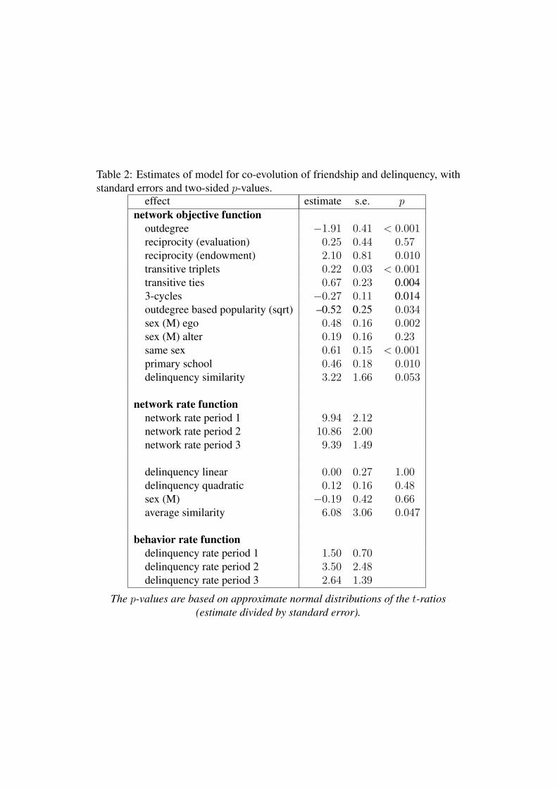
Table 2: Estimates of model for co-evolution of friendship and delinquency, withstandard errors and two-sided p-values.

effect estimate s.e. pnetwork objective function

outdegree −1.91 0.41 < 0.001reciprocity (evaluation) 0.25 0.44 0.57reciprocity (endowment) 2.10 0.81 0.010transitive triplets 0.22 0.03 < 0.001transitive ties 0.67 0.23 0.0043-cycles −0.27 0.11 0.014outdegree based popularity (sqrt) –0.52 0.25 0.034sex (M) ego 0.48 0.16 0.002sex (M) alter 0.19 0.16 0.23same sex 0.61 0.15 < 0.001primary school 0.46 0.18 0.010delinquency similarity 3.22 1.66 0.053

network rate functionnetwork rate period 1 9.94 2.12network rate period 2 10.86 2.00network rate period 3 9.39 1.49

delinquency linear 0.00 0.27 1.00delinquency quadratic 0.12 0.16 0.48sex (M) −0.19 0.42 0.66average similarity 6.08 3.06 0.047

behavior rate functiondelinquency rate period 1 1.50 0.70delinquency rate period 2 3.50 2.48delinquency rate period 3 2.64 1.39

The p-values are based on approximate normal distributions of the t-ratios(estimate divided by standard error).