Embed Size (px)
Citation preview

Introduction to Statistics with GraphPad Prism 8
Anne Segonds-Pichonv2019-03
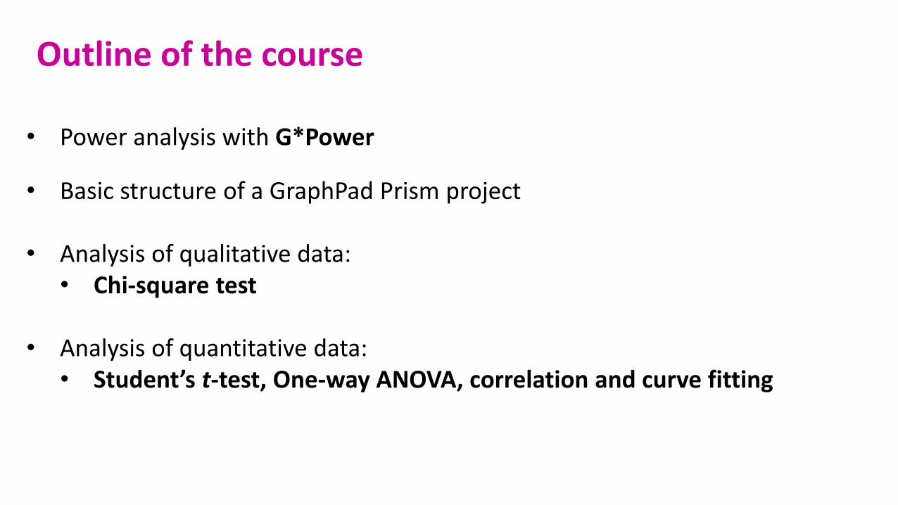
Outline of the course
• Power analysis with G*Power
• Basic structure of a GraphPad Prism project
• Analysis of qualitative data:• Chi-square test
• Analysis of quantitative data:• Student’s t-test, One-way ANOVA, correlation and curve fitting
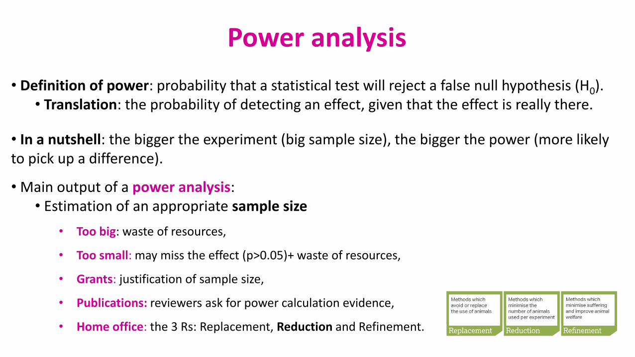
• Definition of power: probability that a statistical test will reject a false null hypothesis (H0).• Translation: the probability of detecting an effect, given that the effect is really there.
• In a nutshell: the bigger the experiment (big sample size), the bigger the power (more likely to pick up a difference).
• Main output of a power analysis:• Estimation of an appropriate sample size
• Too big: waste of resources,
• Too small: may miss the effect (p>0.05)+ waste of resources,
• Grants: justification of sample size,
• Publications: reviewers ask for power calculation evidence,
• Home office: the 3 Rs: Replacement, Reduction and Refinement.
Power analysis
Experimental design
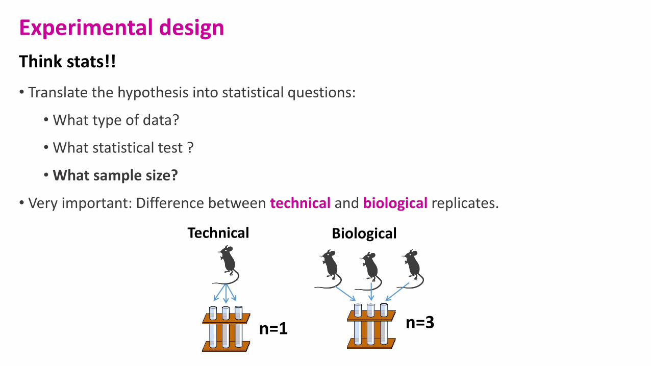
Think stats!!
• Translate the hypothesis into statistical questions:
• What type of data?
• What statistical test ?
• What sample size?
• Very important: Difference between technical and biological replicates.
Biological
n=3
Technical
n=1

A power analysis depends on the relationship between 6 variables:
• the difference of biological interest
• the variability in the data (standard deviation)
• the significance level (5%)
• the desired power of the experiment (80%)
• the sample size
• the alternative hypothesis (ie one or two-sided test)
Effect size
Power analysis
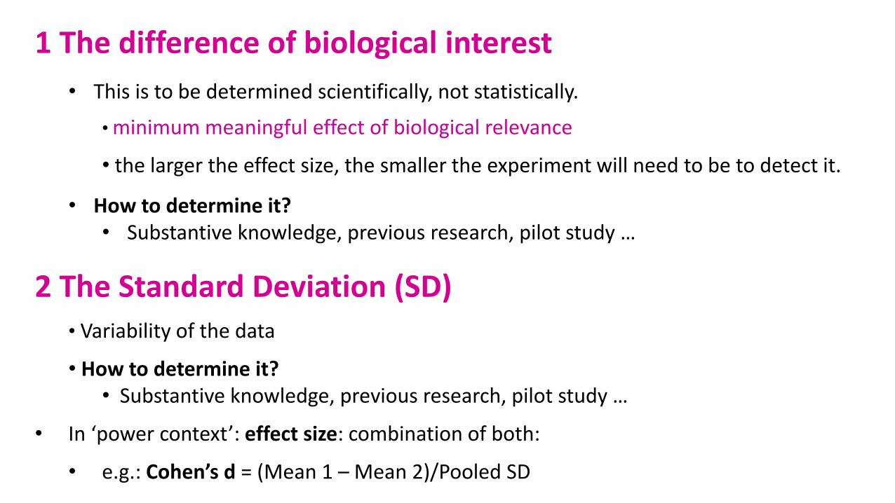
1 The difference of biological interest
• This is to be determined scientifically, not statistically.
• minimum meaningful effect of biological relevance
• the larger the effect size, the smaller the experiment will need to be to detect it.
• How to determine it?• Substantive knowledge, previous research, pilot study …
2 The Standard Deviation (SD)• Variability of the data
• How to determine it?• Substantive knowledge, previous research, pilot study …
• In ‘power context’: effect size: combination of both:
• e.g.: Cohen’s d = (Mean 1 – Mean 2)/Pooled SD
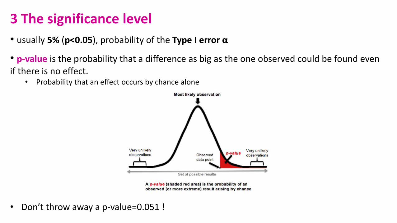
3 The significance level
• usually 5% (p<0.05), probability of the Type I error α
• p-value is the probability that a difference as big as the one observed could be found evenif there is no effect.
• Probability that an effect occurs by chance alone
• Don’t throw away a p-value=0.051 !
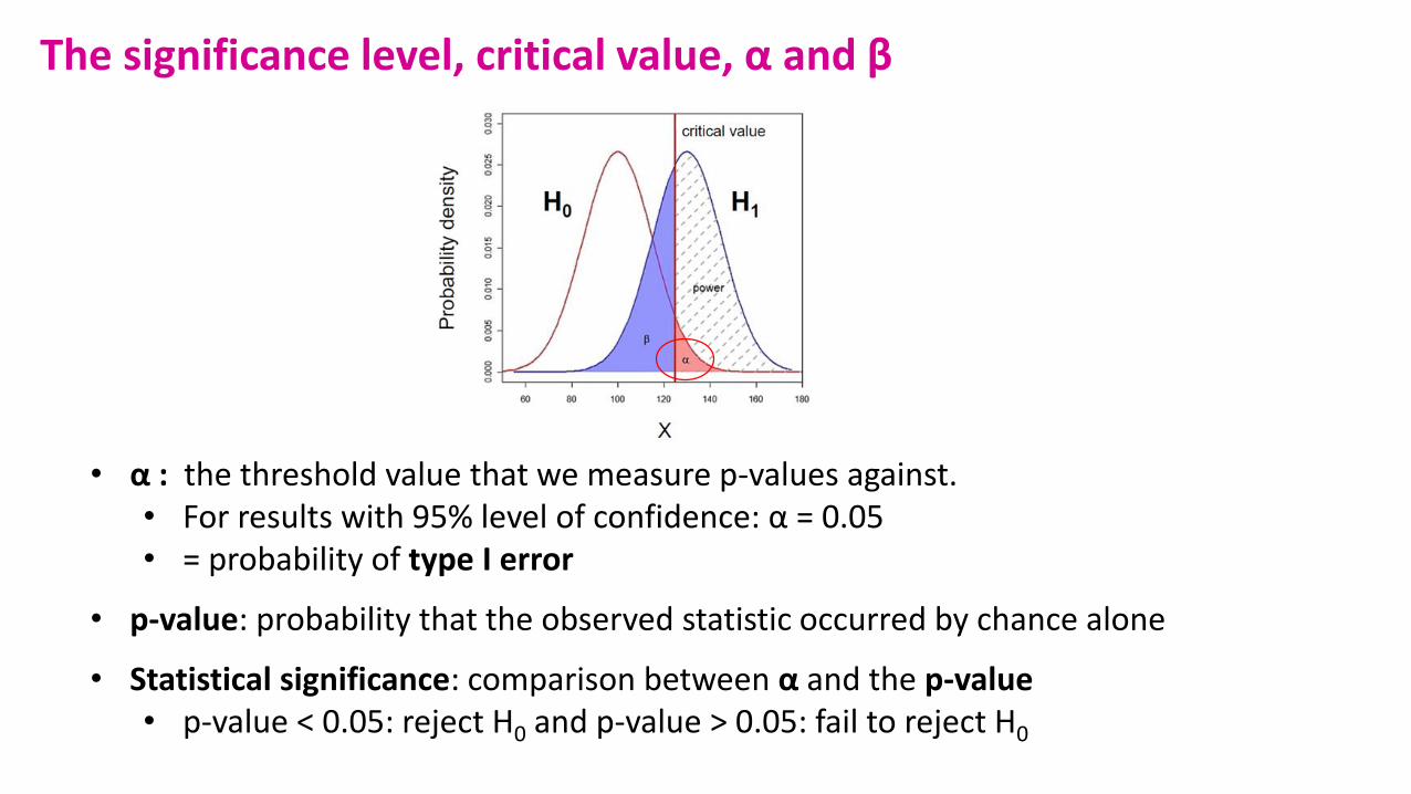
• α : the threshold value that we measure p-values against.• For results with 95% level of confidence: α = 0.05• = probability of type I error
• p-value: probability that the observed statistic occurred by chance alone
• Statistical significance: comparison between α and the p-value• p-value < 0.05: reject H0 and p-value > 0.05: fail to reject H0
The significance level, critical value, α and β
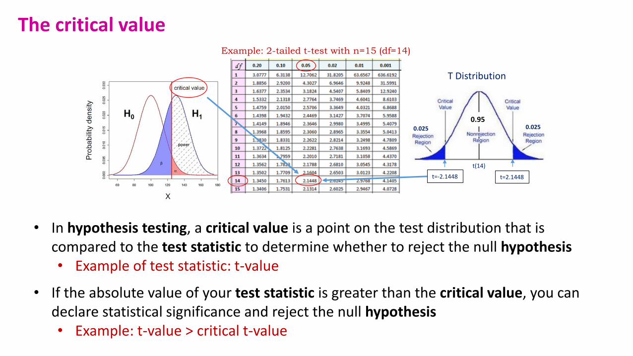
• In hypothesis testing, a critical value is a point on the test distribution that is compared to the test statistic to determine whether to reject the null hypothesis• Example of test statistic: t-value
• If the absolute value of your test statistic is greater than the critical value, you can declare statistical significance and reject the null hypothesis• Example: t-value > critical t-value
Example: 2-tailed t-test with n=15 (df=14)
T Distribution
0.950.025 0.025
t=-2.1448 t=2.1448
t(14)
The critical value
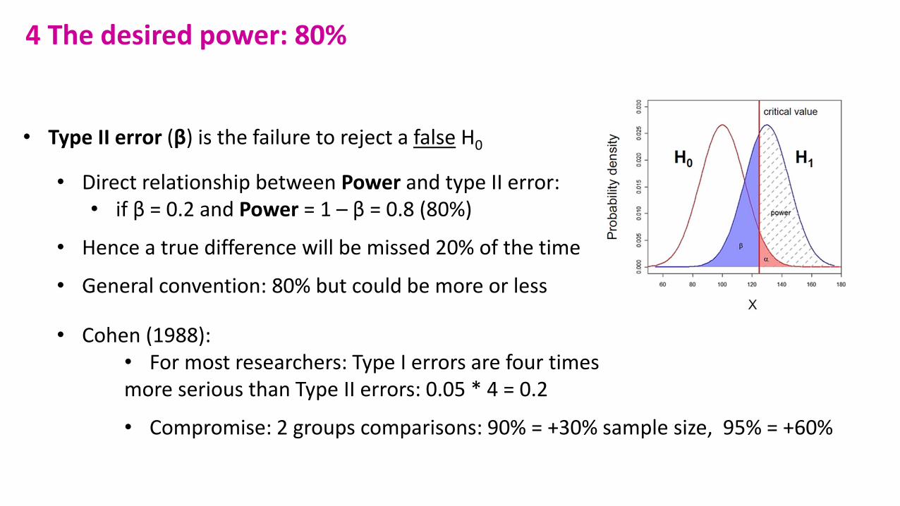
• Type II error (β) is the failure to reject a false H0
• Direct relationship between Power and type II error: • if β = 0.2 and Power = 1 – β = 0.8 (80%)
• Hence a true difference will be missed 20% of the time
• General convention: 80% but could be more or less
• Cohen (1988): • For most researchers: Type I errors are four times more serious than Type II errors: 0.05 * 4 = 0.2
• Compromise: 2 groups comparisons: 90% = +30% sample size, 95% = +60%
4 The desired power: 80%
5 The sample size: the bigger the better?
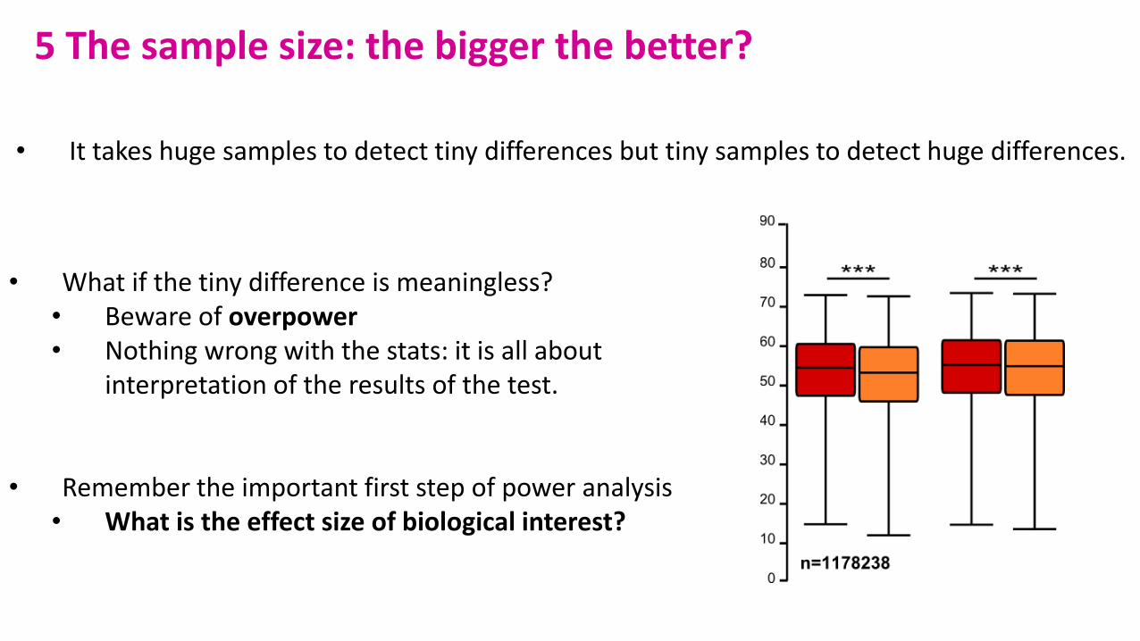
• What if the tiny difference is meaningless?• Beware of overpower• Nothing wrong with the stats: it is all about
interpretation of the results of the test.
• Remember the important first step of power analysis• What is the effect size of biological interest?
• It takes huge samples to detect tiny differences but tiny samples to detect huge differences.
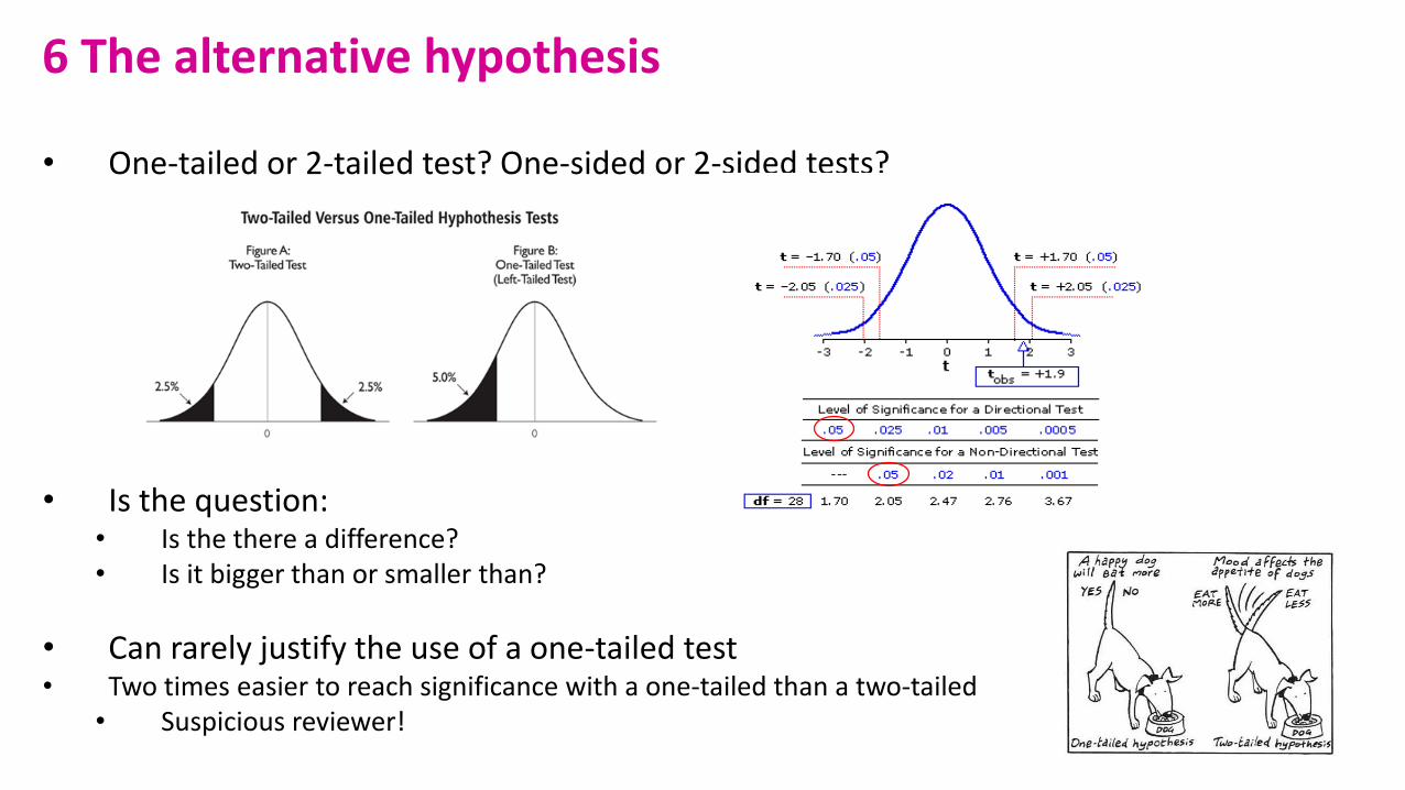
• One-tailed or 2-tailed test? One-sided or 2-sided tests?
• Is the question:• Is the there a difference?• Is it bigger than or smaller than?
• Can rarely justify the use of a one-tailed test• Two times easier to reach significance with a one-tailed than a two-tailed
• Suspicious reviewer!
6 The alternative hypothesis
To recapitulate:
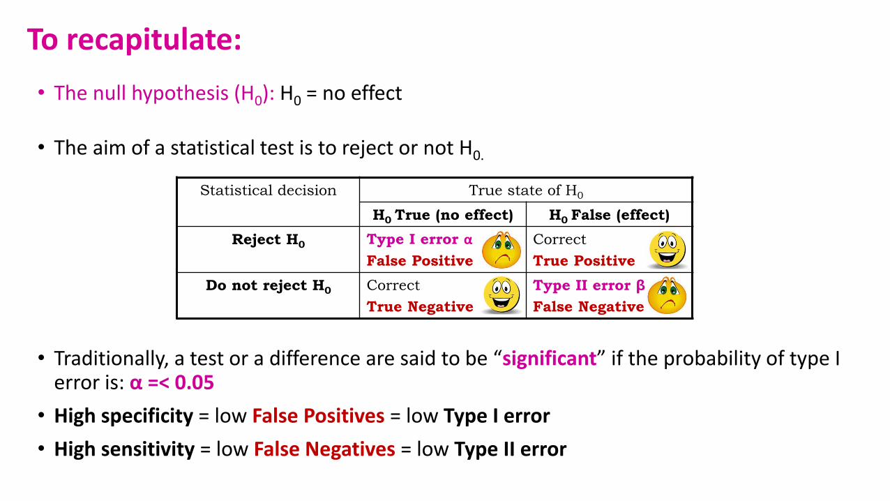
• The null hypothesis (H0): H0 = no effect
• The aim of a statistical test is to reject or not H0.
• Traditionally, a test or a difference are said to be “significant” if the probability of type I error is: α =< 0.05
• High specificity = low False Positives = low Type I error
• High sensitivity = low False Negatives = low Type II error
Statistical decision True state of H0
H0 True (no effect) H0 False (effect)
Reject H0 Type I error α
False Positive
Correct
True Positive
Do not reject H0 Correct
True Negative
Type II error β
False Negative
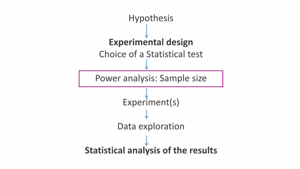
Hypothesis
Experimental designChoice of a Statistical test
Power analysis: Sample size
Experiment(s)
Data exploration
Statistical analysis of the results
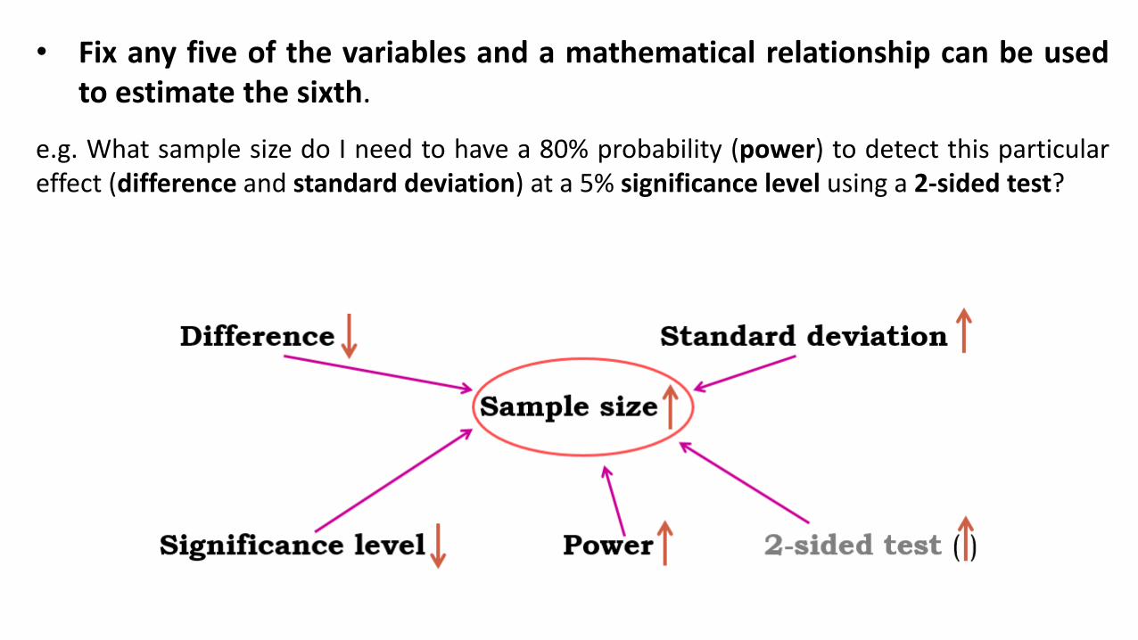
• Fix any five of the variables and a mathematical relationship can be usedto estimate the sixth.
e.g. What sample size do I need to have a 80% probability (power) to detect this particulareffect (difference and standard deviation) at a 5% significance level using a 2-sided test?
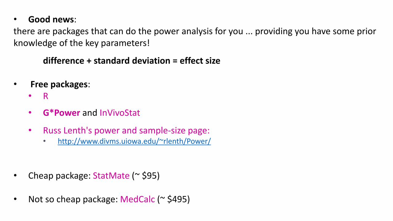
• Good news:there are packages that can do the power analysis for you ... providing you have some priorknowledge of the key parameters!
difference + standard deviation = effect size
• Free packages:• R
• G*Power and InVivoStat
• Russ Lenth's power and sample-size page:• http://www.divms.uiowa.edu/~rlenth/Power/
• Cheap package: StatMate (~ $95)
• Not so cheap package: MedCalc (~ $495)
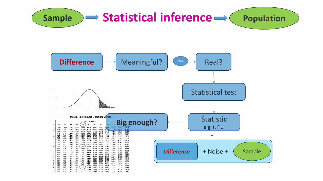
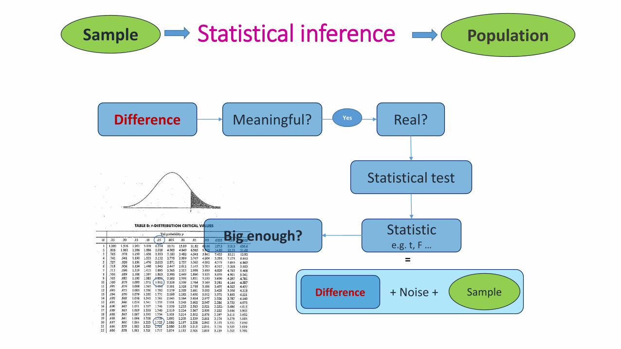
+ Noise +
Statistical inference
Difference Meaningful? Real?
Statistical test
Statistice.g. t, F …
Big enough?
Difference
Sample Population
Sample
=
Yes

Qualitative data
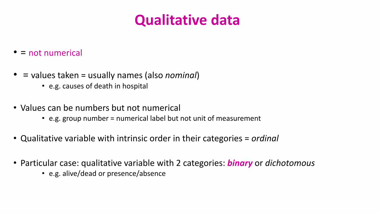
Qualitative data
• = not numerical
• = values taken = usually names (also nominal)• e.g. causes of death in hospital
• Values can be numbers but not numerical• e.g. group number = numerical label but not unit of measurement
• Qualitative variable with intrinsic order in their categories = ordinal
• Particular case: qualitative variable with 2 categories: binary or dichotomous• e.g. alive/dead or presence/absence
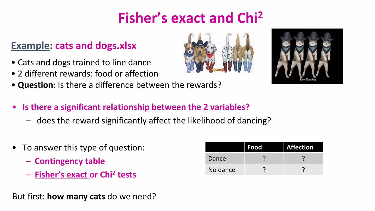
Example: cats and dogs.xlsx
• Cats and dogs trained to line dance• 2 different rewards: food or affection• Question: Is there a difference between the rewards?
• Is there a significant relationship between the 2 variables?
– does the reward significantly affect the likelihood of dancing?
• To answer this type of question:
– Contingency table
– Fisher’s exact or Chi2 tests
Fisher’s exact and Chi2
Food Affection
Dance ? ?
No dance ? ?
But first: how many cats do we need?
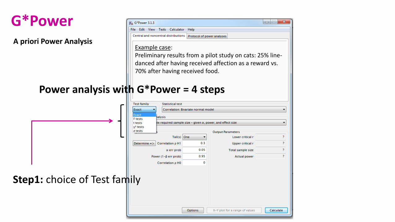
G*Power
Step1: choice of Test family
Power analysis with G*Power = 4 steps
Example case:Preliminary results from a pilot study on cats: 25% line-danced after having received affection as a reward vs. 70% after having received food.
A priori Power Analysis

Step 2 : choice of Statistical test
Fisher’s exact test or Chi-square for 2x2 tables
G*Power
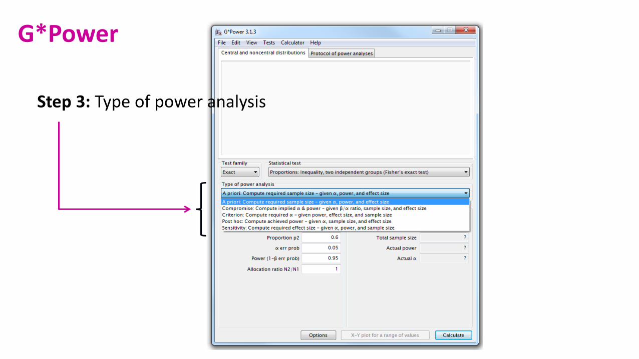
Step 3: Type of power analysis
G*Power
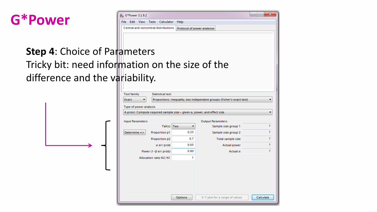
Step 4: Choice of ParametersTricky bit: need information on the size of the difference and the variability.
G*Power
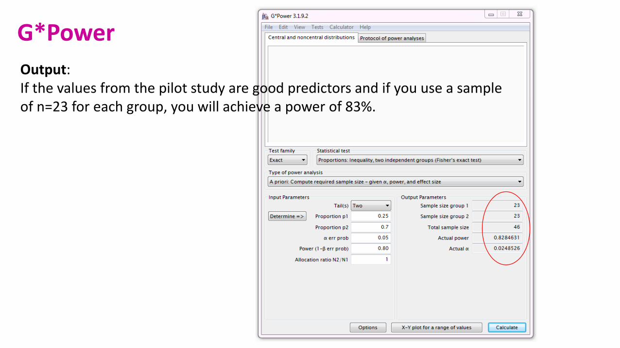
Output: If the values from the pilot study are good predictors and if you use a sample of n=23 for each group, you will achieve a power of 83%.
G*Power
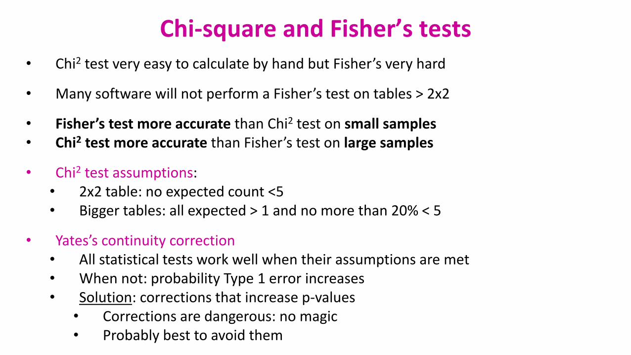
Chi-square and Fisher’s tests• Chi2 test very easy to calculate by hand but Fisher’s very hard
• Many software will not perform a Fisher’s test on tables > 2x2
• Fisher’s test more accurate than Chi2 test on small samples• Chi2 test more accurate than Fisher’s test on large samples
• Chi2 test assumptions:• 2x2 table: no expected count <5• Bigger tables: all expected > 1 and no more than 20% < 5
• Yates’s continuity correction• All statistical tests work well when their assumptions are met• When not: probability Type 1 error increases• Solution: corrections that increase p-values
• Corrections are dangerous: no magic• Probably best to avoid them
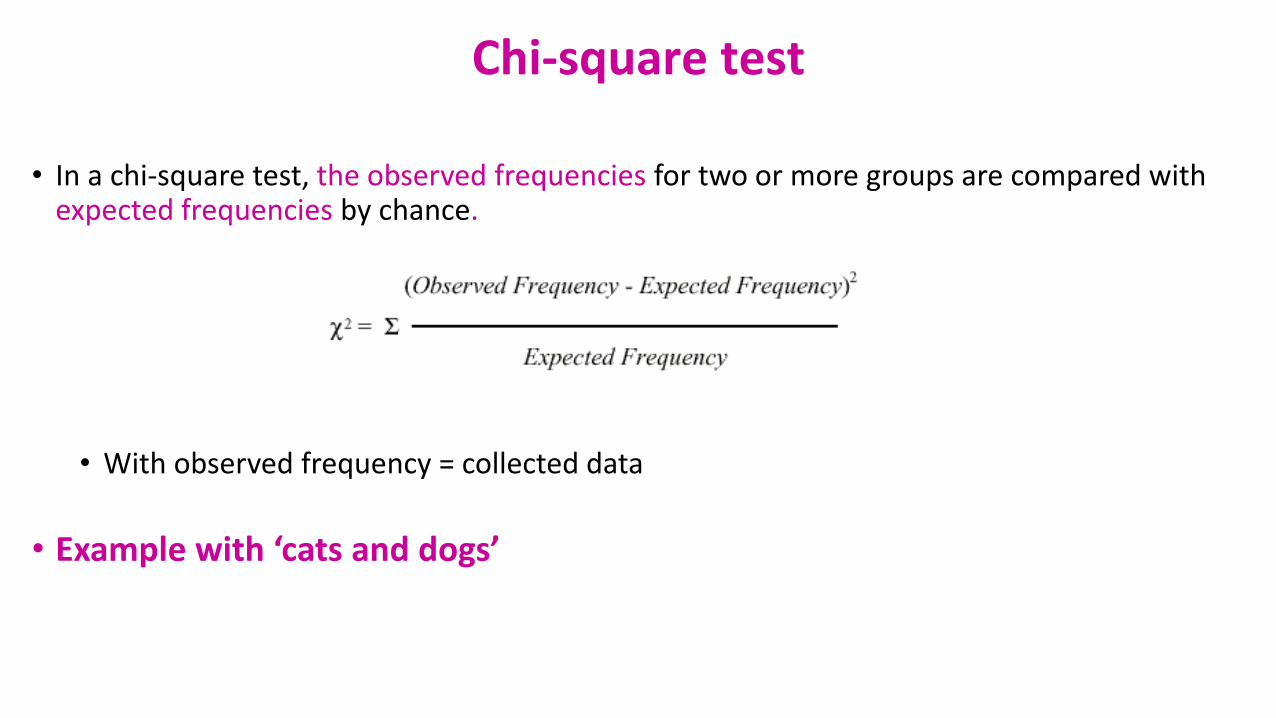
• In a chi-square test, the observed frequencies for two or more groups are compared withexpected frequencies by chance.
• With observed frequency = collected data
• Example with ‘cats and dogs’
Chi-square test
Did they dance? * Type of Training * Animal Crosstabulation
26 6 32
81.3% 18.8% 100.0%
6 30 36
16.7% 83.3% 100.0%
32 36 68
47.1% 52.9% 100.0%
23 24 47
48.9% 51.1% 100.0%
9 10 19
47.4% 52.6% 100.0%
32 34 66
48.5% 51.5% 100.0%
Count
% within Did they dance?
Count
% within Did they dance?
Count
% within Did they dance?
Count
% within Did they dance?
Count
% within Did they dance?
Count
% within Did they dance?
Yes
No
Did they
dance?
Total
Yes
No
Did they
dance?
Total
Animal
Cat
Dog
Food as
Reward
Af fect ion as
Reward
Type of Training
Total
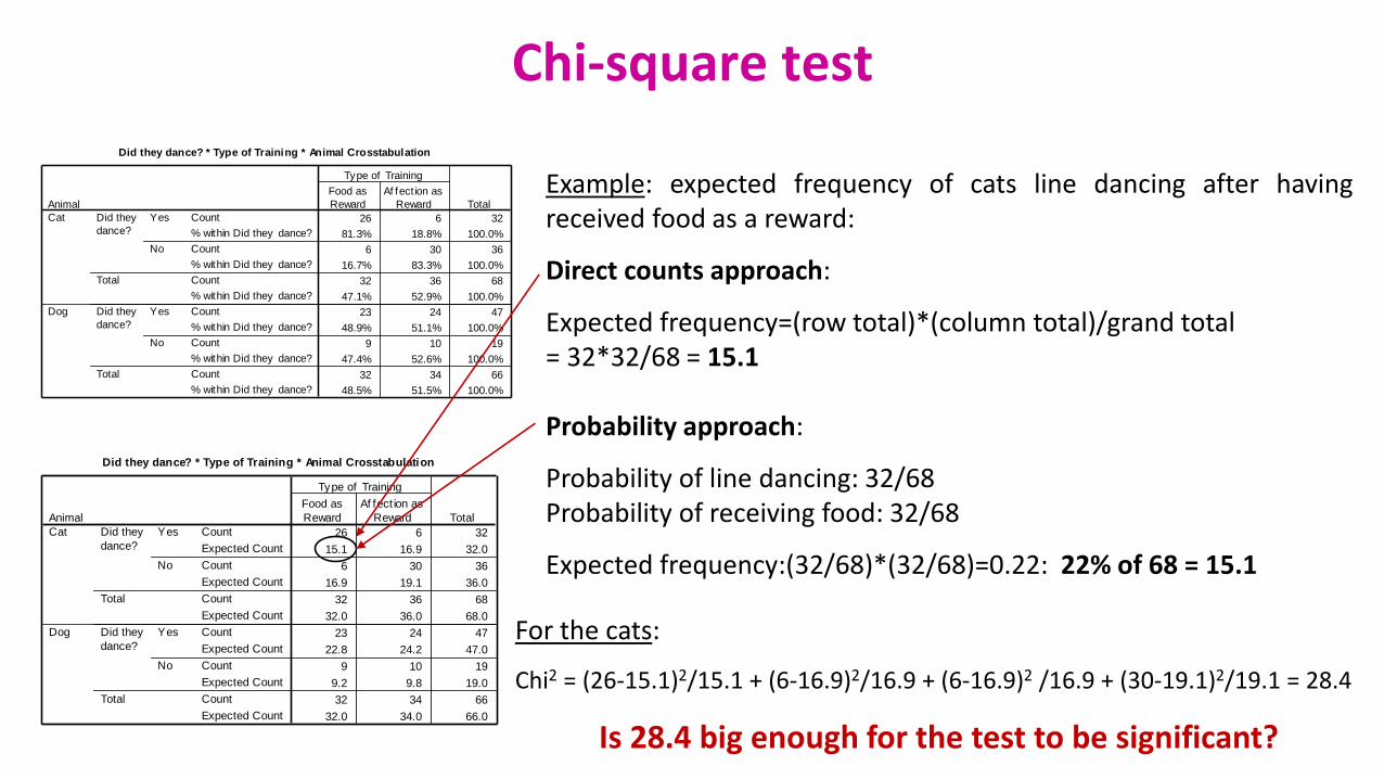
Example: expected frequency of cats line dancing after havingreceived food as a reward:
Direct counts approach:
Expected frequency=(row total)*(column total)/grand total= 32*32/68 = 15.1
Probability approach:
Probability of line dancing: 32/68Probability of receiving food: 32/68
Expected frequency:(32/68)*(32/68)=0.22: 22% of 68 = 15.1
Did they dance? * Type of Training * Animal Crosstabulation
26 6 32
15.1 16.9 32.0
6 30 36
16.9 19.1 36.0
32 36 68
32.0 36.0 68.0
23 24 47
22.8 24.2 47.0
9 10 19
9.2 9.8 19.0
32 34 66
32.0 34.0 66.0
Count
Expected Count
Count
Expected Count
Count
Expected Count
Count
Expected Count
Count
Expected Count
Count
Expected Count
Yes
No
Did they
dance?
Total
Yes
No
Did they
dance?
Total
Animal
Cat
Dog
Food as
Reward
Af fect ion as
Reward
Type of Training
Total
For the cats:
Chi2 = (26-15.1)2/15.1 + (6-16.9)2/16.9 + (6-16.9)2 /16.9 + (30-19.1)2/19.1 = 28.4
Is 28.4 big enough for the test to be significant?
Chi-square test
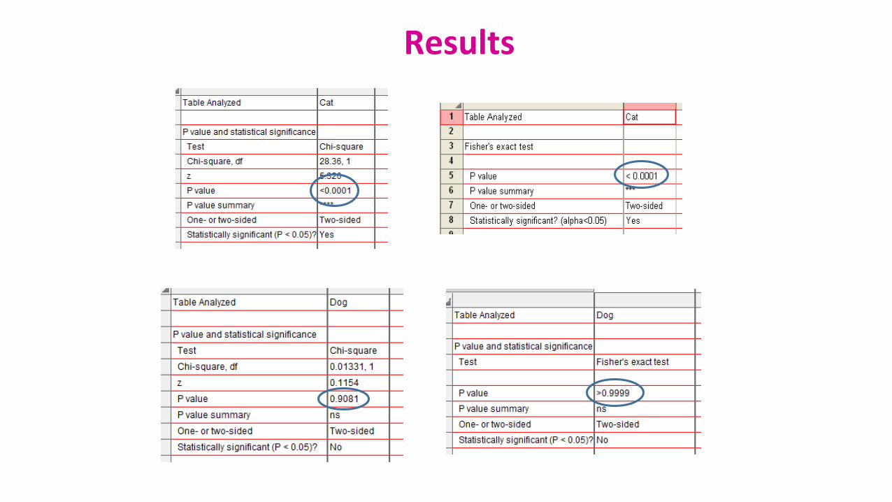
Results
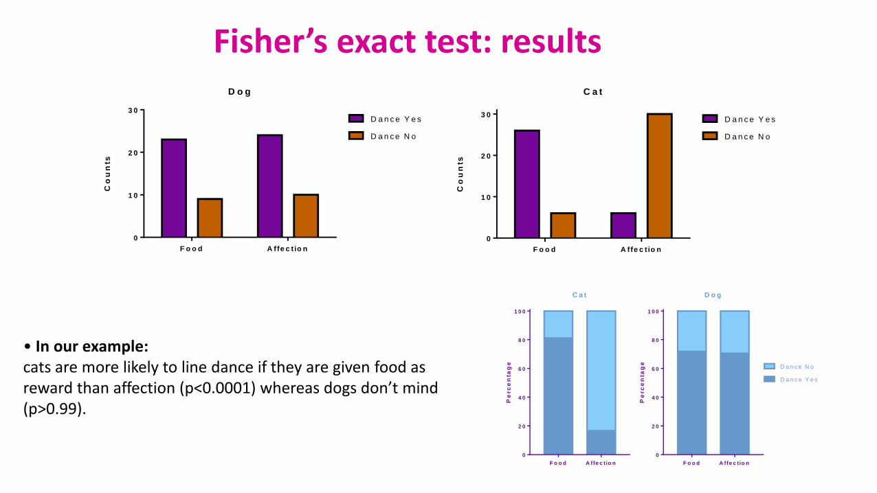
Fisher’s exact test: results
• In our example: cats are more likely to line dance if they are given food as reward than affection (p<0.0001) whereas dogs don’t mind (p>0.99).
F o o d A ffe c t io n
0
2 0
4 0
6 0
8 0
1 0 0
C a t
Pe
rc
en
tag
e
F o o d A ffe c t io n
0
2 0
4 0
6 0
8 0
1 0 0
D o g
Pe
rc
en
tag
e
D a n c e Y e s
D a n c e N o
D o g
F o o d A ffe c t io n
0
1 0
2 0
3 0
D a n c e Y e s
D a n c e N o
Co
un
ts
C a t
F o o d A ffe c t io n
0
1 0
2 0
3 0D a n c e Y e s
D a n c e N o
Co
un
ts

Quantitative data
Quantitative data
• They take numerical values (units of measurement)
• Discrete: obtained by counting• Example: number of students in a class
• values vary by finite specific steps
• or continuous: obtained by measuring• Example: height of students in a class
• any values
• They can be described by a series of parameters:
• Mean, variance, standard deviation, standard error and confidence interval
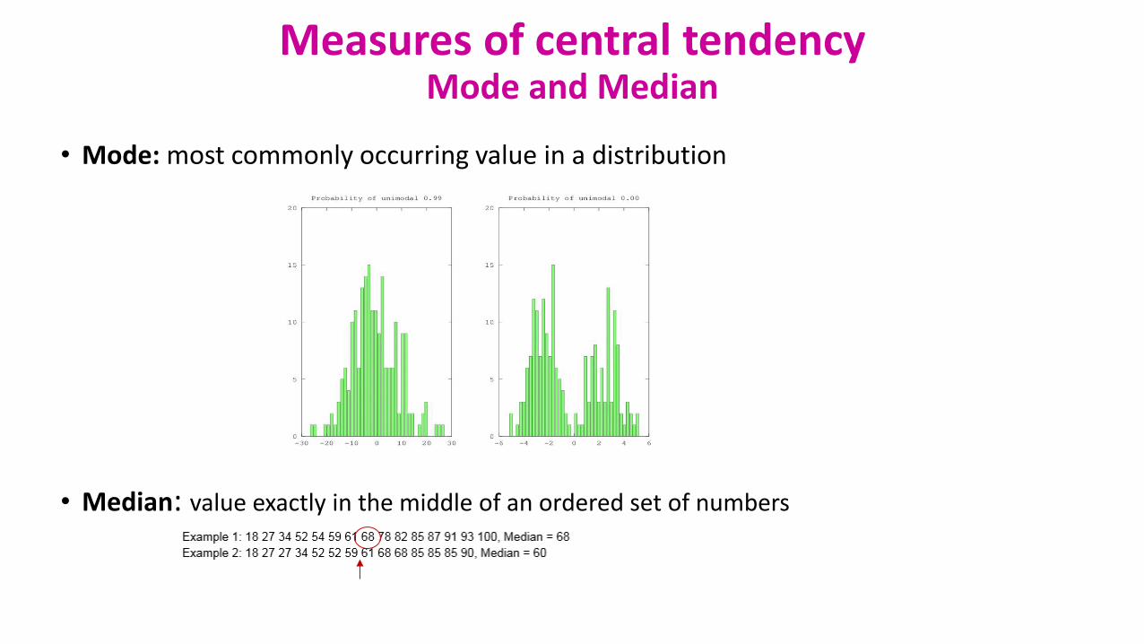
Measures of central tendencyMode and Median
• Mode: most commonly occurring value in a distribution
• Median: value exactly in the middle of an ordered set of numbers

• Definition: average of all values in a column
• It can be considered as a model because it summaries the data
• Example: a group of 5 lecturers: number of friends of each members of the group: 1, 2, 3, 3 and 4• Mean: (1+2+3+3+4)/5 = 2.6 friends per person
• Clearly an hypothetical value
• How can we know that it is an accurate model?
• Difference between the real data and the model created
Measures of central tendencyMean
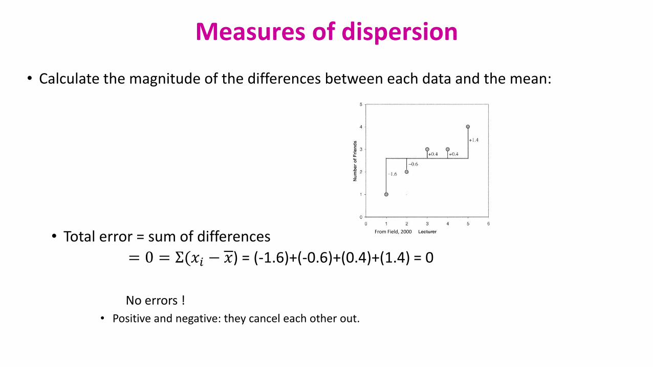
• Calculate the magnitude of the differences between each data and the mean:
• Total error = sum of differences
= 0 = Σ(𝑥𝑖 − 𝑥) = (-1.6)+(-0.6)+(0.4)+(1.4) = 0
No errors !
• Positive and negative: they cancel each other out.
From Field, 2000
Measures of dispersion
Sum of Squared errors (SS)
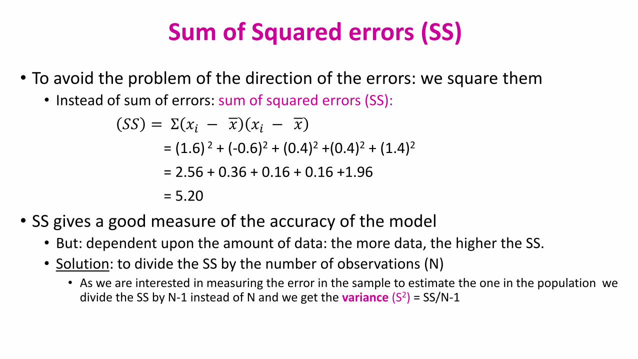
• To avoid the problem of the direction of the errors: we square them• Instead of sum of errors: sum of squared errors (SS):
𝑆𝑆 = Σ 𝑥𝑖 − 𝑥 𝑥𝑖 − 𝑥
= (1.6) 2 + (-0.6)2 + (0.4)2 +(0.4)2 + (1.4)2
= 2.56 + 0.36 + 0.16 + 0.16 +1.96
= 5.20
• SS gives a good measure of the accuracy of the model• But: dependent upon the amount of data: the more data, the higher the SS.
• Solution: to divide the SS by the number of observations (N)• As we are interested in measuring the error in the sample to estimate the one in the population we
divide the SS by N-1 instead of N and we get the variance (S2) = SS/N-1
Variance and standard deviation
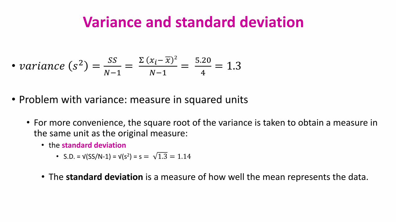
• 𝑣𝑎𝑟𝑖𝑎𝑛𝑐𝑒 𝑠2 =𝑆𝑆
𝑁−1=
Σ 𝑥𝑖− 𝑥 2
𝑁−1=
5.20
4= 1.3
• Problem with variance: measure in squared units
• For more convenience, the square root of the variance is taken to obtain a measure in the same unit as the original measure: • the standard deviation
• S.D. = √(SS/N-1) = √(s2) = s = 1.3 = 1.14
• The standard deviation is a measure of how well the mean represents the data.
Standard deviation
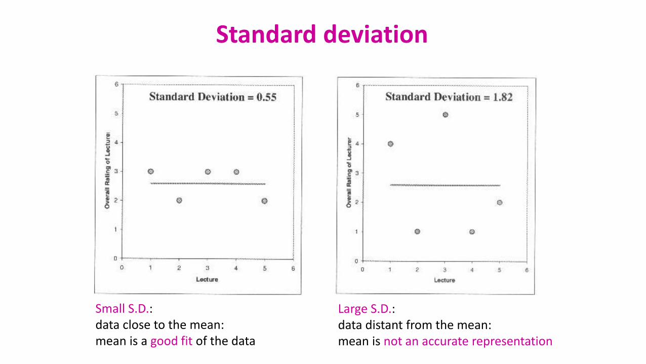
Small S.D.: data close to the mean: mean is a good fit of the data
Large S.D.: data distant from the mean: mean is not an accurate representation
SD and SEM (SEM = SD/√N)
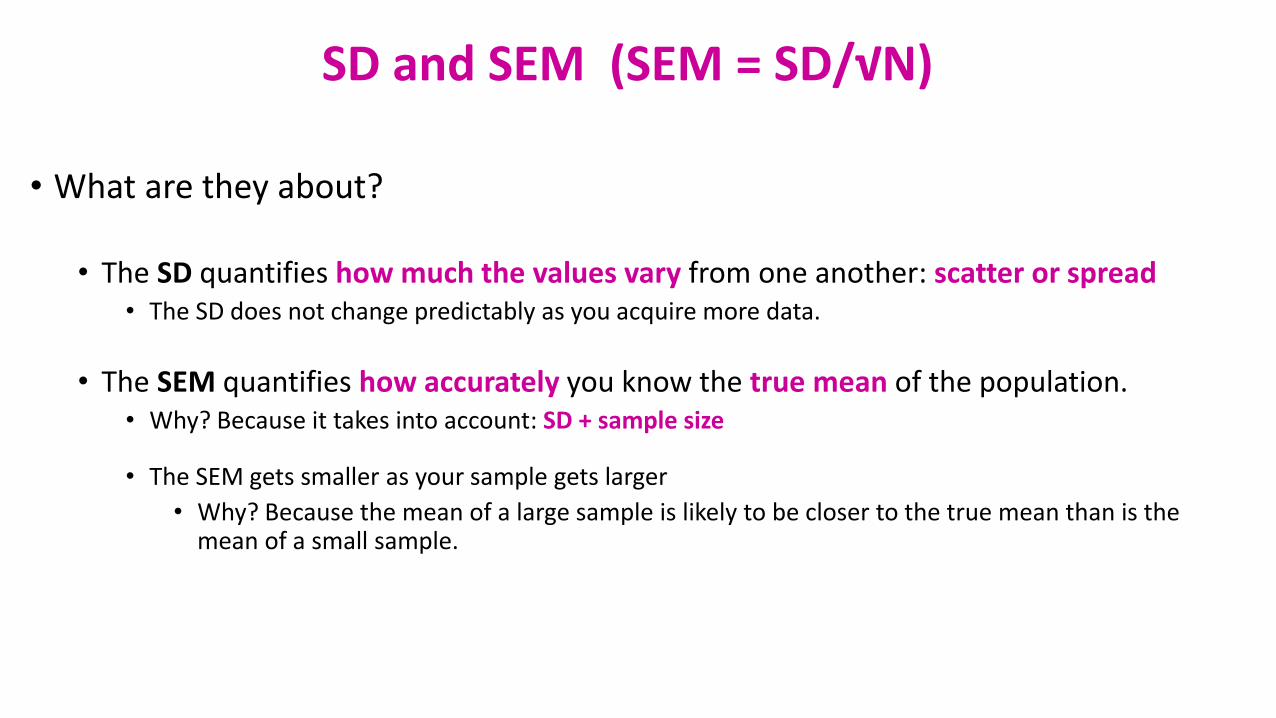
• What are they about?
• The SD quantifies how much the values vary from one another: scatter or spread • The SD does not change predictably as you acquire more data.
• The SEM quantifies how accurately you know the true mean of the population. • Why? Because it takes into account: SD + sample size
• The SEM gets smaller as your sample gets larger
• Why? Because the mean of a large sample is likely to be closer to the true mean than is the mean of a small sample.
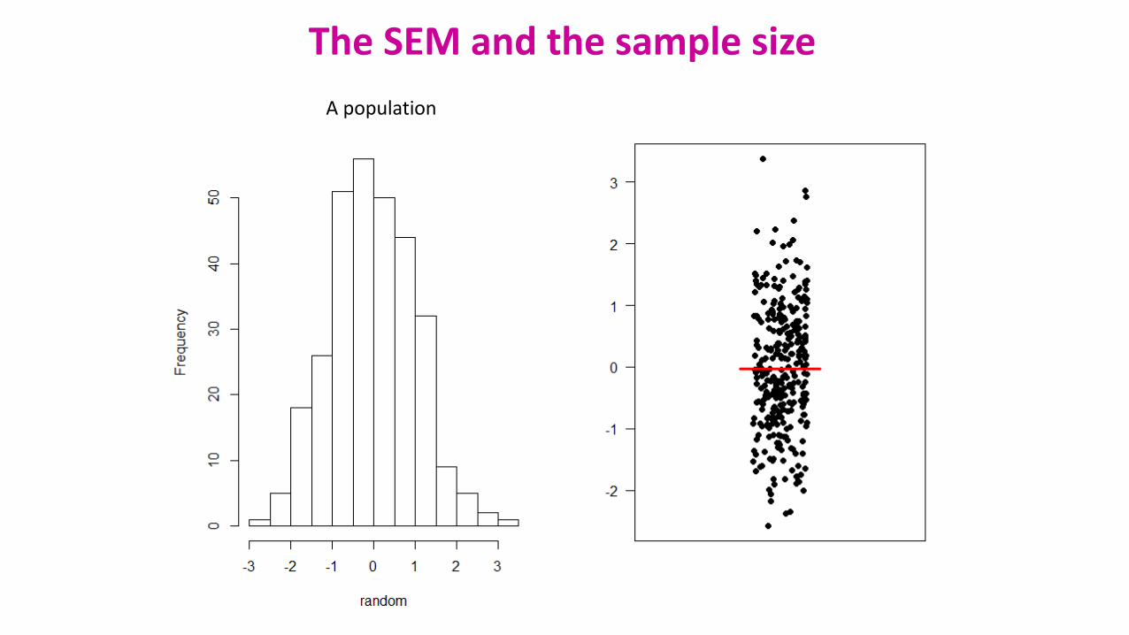
The SEM and the sample size
A population
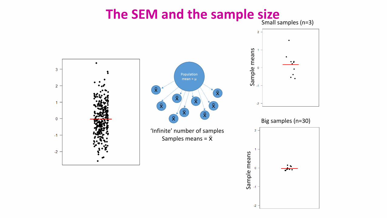
Small samples (n=3)
Big samples (n=30)
‘Infinite’ number of samplesSamples means =
Sam
ple
mea
ns
Sam
ple
mea
ns
The SEM and the sample size
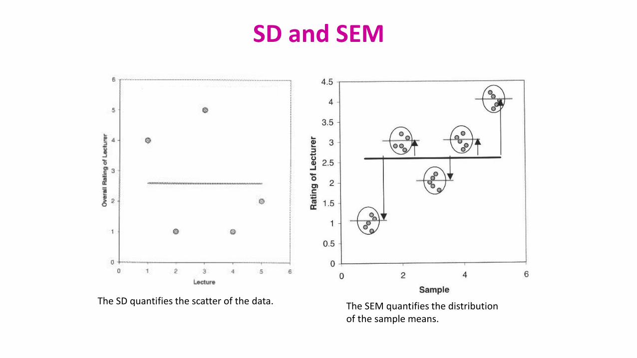
SD and SEM
The SD quantifies the scatter of the data. The SEM quantifies the distribution of the sample means.
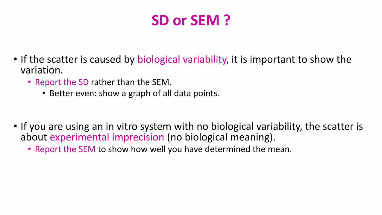
SD or SEM ?
• If the scatter is caused by biological variability, it is important to show the variation. • Report the SD rather than the SEM.
• Better even: show a graph of all data points.
• If you are using an in vitro system with no biological variability, the scatter is about experimental imprecision (no biological meaning). • Report the SEM to show how well you have determined the mean.
Confidence interval
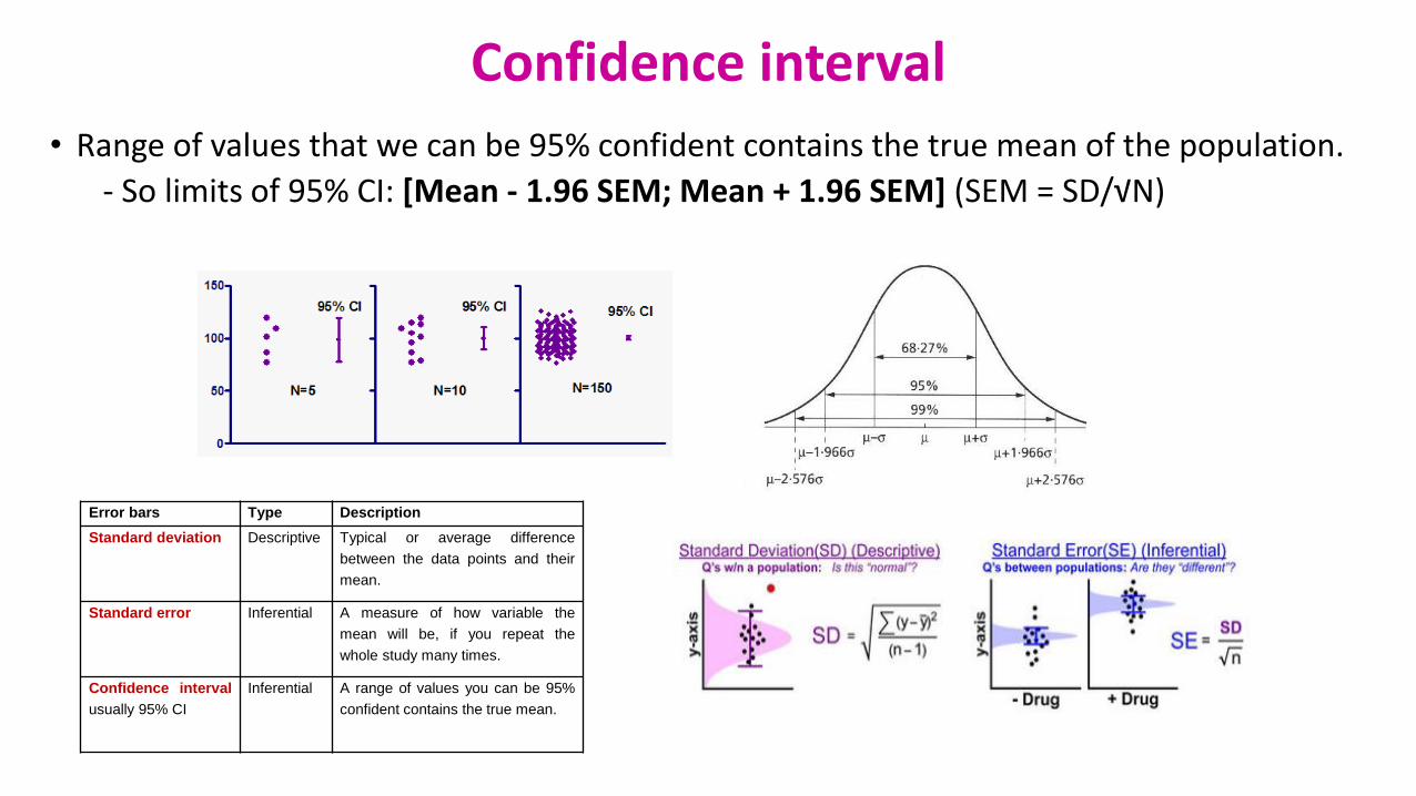
• Range of values that we can be 95% confident contains the true mean of the population.
- So limits of 95% CI: [Mean - 1.96 SEM; Mean + 1.96 SEM] (SEM = SD/√N)
Error bars Type Description
Standard deviation Descriptive Typical or average difference
between the data points and their
mean.
Standard error Inferential A measure of how variable the
mean will be, if you repeat the
whole study many times.
Confidence interval
usually 95% CI
Inferential A range of values you can be 95%
confident contains the true mean.
Analysis of Quantitative Data
• Choose the correct statistical test to answer your question:
• They are 2 types of statistical tests:
• Parametric tests with 4 assumptions to be met by the data,
• Non-parametric tests with no or few assumptions (e.g. Mann-Whitney test) and/or for qualitative data (e.g. Fisher’s exact and χ2 tests).
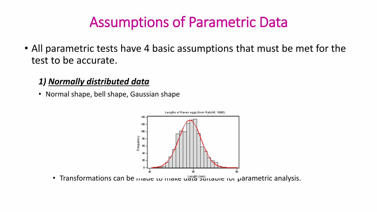
• All parametric tests have 4 basic assumptions that must be met for the test to be accurate.
1) Normally distributed data
• Normal shape, bell shape, Gaussian shape
• Transformations can be made to make data suitable for parametric analysis.
Assumptions of Parametric Data
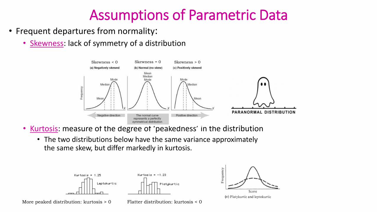
• Frequent departures from normality:• Skewness: lack of symmetry of a distribution
• Kurtosis: measure of the degree of ‘peakedness’ in the distribution• The two distributions below have the same variance approximately
the same skew, but differ markedly in kurtosis.
Flatter distribution: kurtosis < 0More peaked distribution: kurtosis > 0
Skewness > 0Skewness < 0 Skewness = 0
Assumptions of Parametric Data
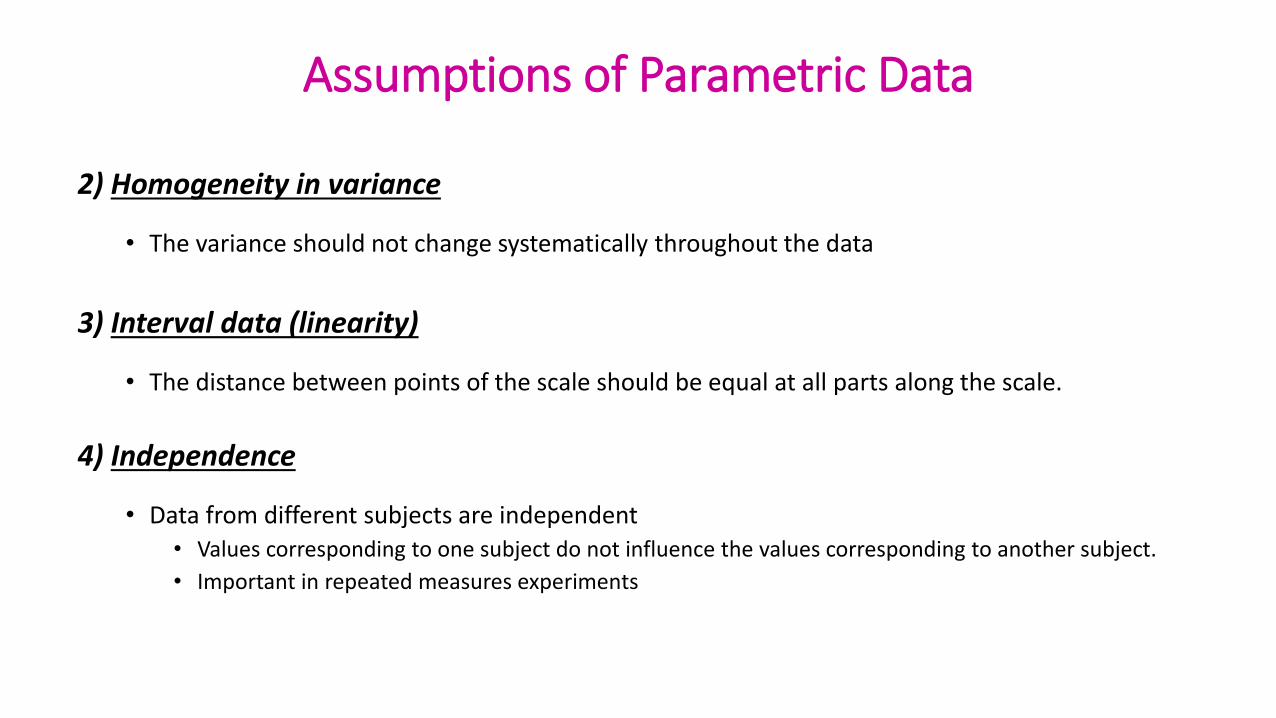
2) Homogeneity in variance
• The variance should not change systematically throughout the data
3) Interval data (linearity)
• The distance between points of the scale should be equal at all parts along the scale.
4) Independence
• Data from different subjects are independent• Values corresponding to one subject do not influence the values corresponding to another subject.
• Important in repeated measures experiments
Assumptions of Parametric Data
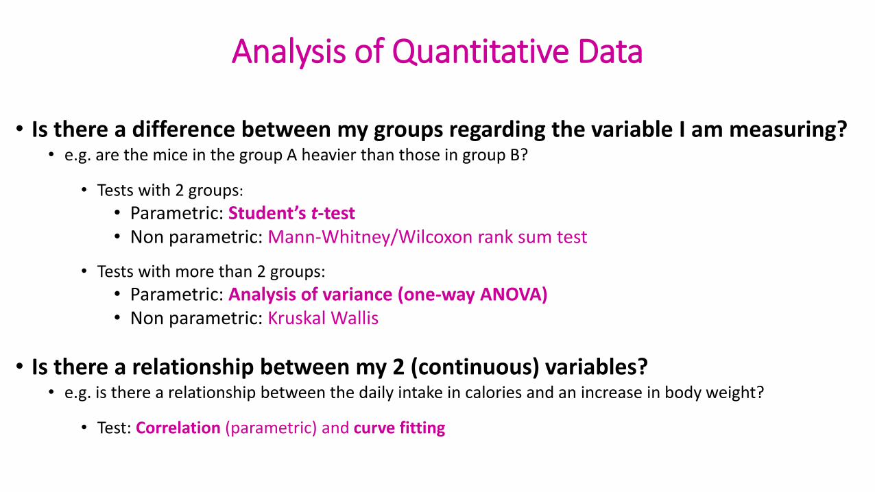
• Is there a difference between my groups regarding the variable I am measuring?• e.g. are the mice in the group A heavier than those in group B?
• Tests with 2 groups:
• Parametric: Student’s t-test• Non parametric: Mann-Whitney/Wilcoxon rank sum test
• Tests with more than 2 groups:
• Parametric: Analysis of variance (one-way ANOVA)• Non parametric: Kruskal Wallis
• Is there a relationship between my 2 (continuous) variables?• e.g. is there a relationship between the daily intake in calories and an increase in body weight?
• Test: Correlation (parametric) and curve fitting
Analysis of Quantitative Data
+ Noise +
Statistical inference
Difference Meaningful? Real?
Statistical test
Statistice.g. t, F …
Big enough?
Difference
Sample Population
Sample
=
Yes
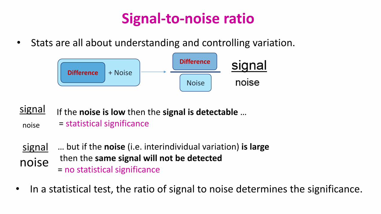
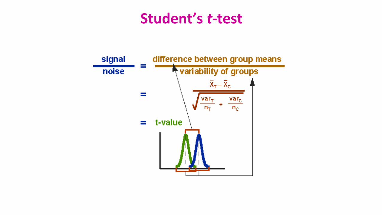
• Stats are all about understanding and controlling variation.
signal
noise
signal
noise
If the noise is low then the signal is detectable …= statistical significance
… but if the noise (i.e. interindividual variation) is largethen the same signal will not be detected = no statistical significance
• In a statistical test, the ratio of signal to noise determines the significance.
+ NoiseDifference
Difference
Noise
Signal-to-noise ratio
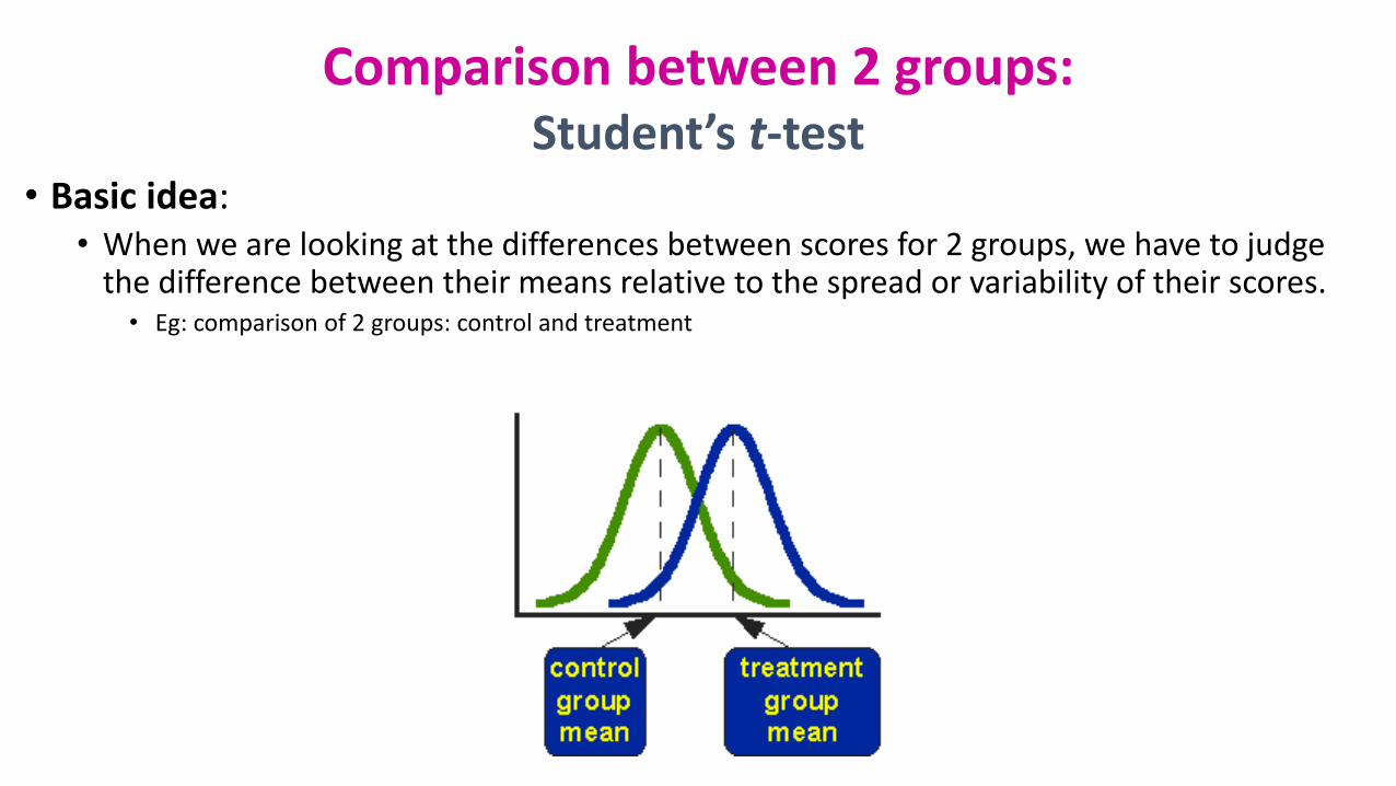
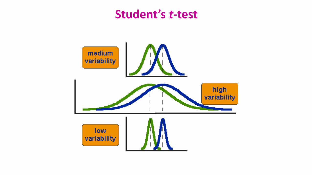
• Basic idea: • When we are looking at the differences between scores for 2 groups, we have to judge
the difference between their means relative to the spread or variability of their scores.• Eg: comparison of 2 groups: control and treatment
Comparison between 2 groups: Student’s t-test
Student’s t-test
Student’s t-test
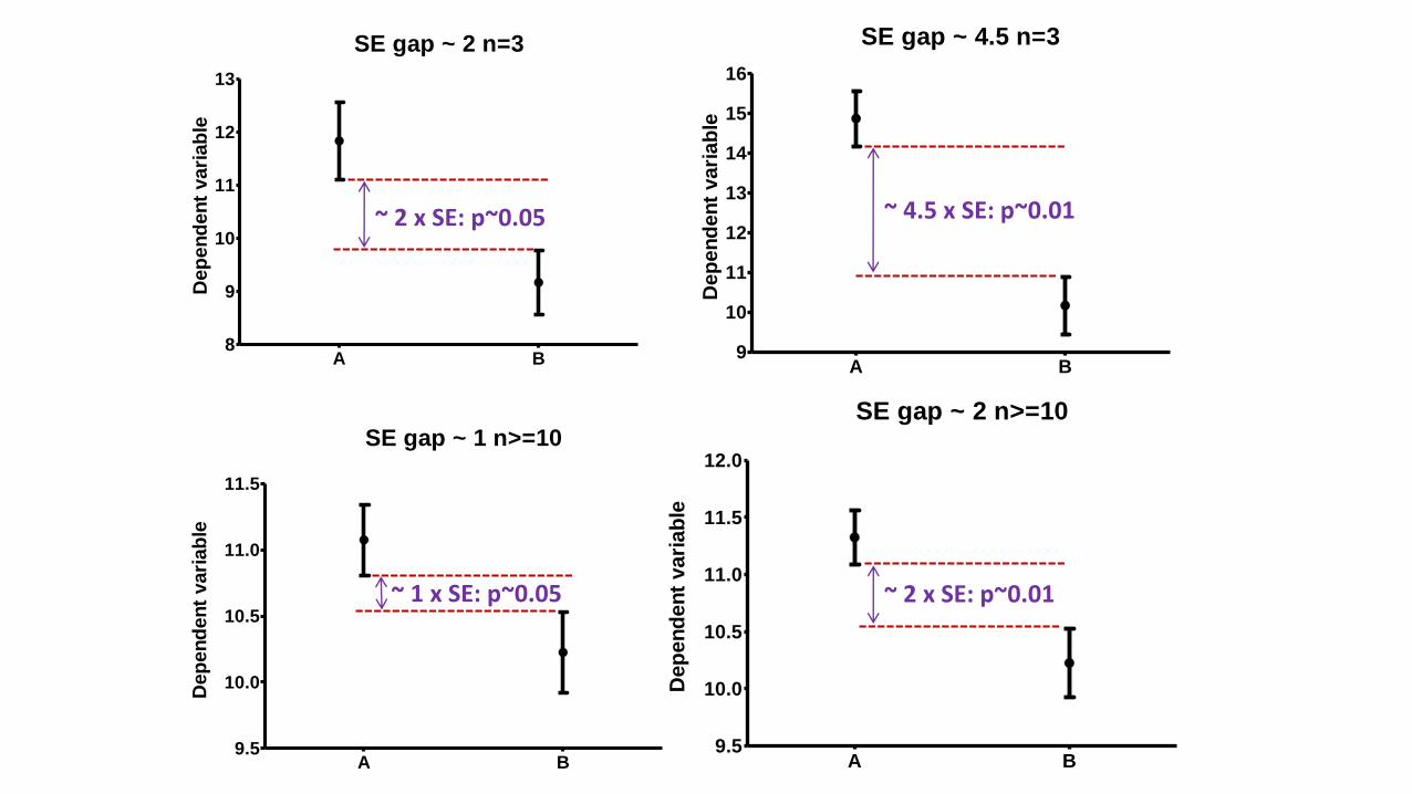
SE gap ~ 2 n=3
A B8
9
10
11
12
13
Dep
en
den
t vari
ab
le
SE gap ~ 4.5 n=3
A B9
10
11
12
13
14
15
16
Dep
en
den
t vari
ab
le
SE gap ~ 1 n>=10
A B9.5
10.0
10.5
11.0
11.5
Dep
en
den
t vari
ab
le
SE gap ~ 2 n>=10
A B9.5
10.0
10.5
11.0
11.5
12.0
Dep
en
den
t vari
ab
le
~ 2 x SE: p~0.05
~ 1 x SE: p~0.05 ~ 2 x SE: p~0.01
~ 4.5 x SE: p~0.01
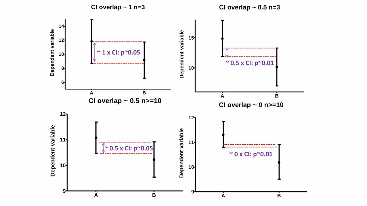
CI overlap ~ 1 n=3
A B
6
8
10
12
14
Dep
en
den
t vari
ab
le
CI overlap ~ 0.5 n=3
A B
10
15
Dep
en
den
t vari
ab
le
CI overlap ~ 0.5 n>=10
A B9
10
11
12
Dep
en
den
t vari
ab
le
CI overlap ~ 0 n>=10
A B9
10
11
12
Dep
en
den
t vari
ab
le
~ 1 x CI: p~0.05
~ 0.5 x CI: p~0.05
~ 0.5 x CI: p~0.01
~ 0 x CI: p~0.01

• 3 types:
• Independent t-test• compares means for two independent groups of cases.
• Paired t-test• looks at the difference between two variables for a single group:
• the second ‘sample’ of values comes from the same subjects (mouse, petri dish …).
• One-Sample t-test • tests whether the mean of a single variable differs from a specified constant (often 0)
Student’s t-test
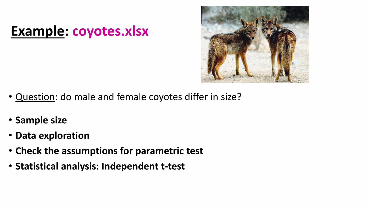
Example: coyotes.xlsx
• Question: do male and female coyotes differ in size?
• Sample size
• Data exploration
• Check the assumptions for parametric test
• Statistical analysis: Independent t-test
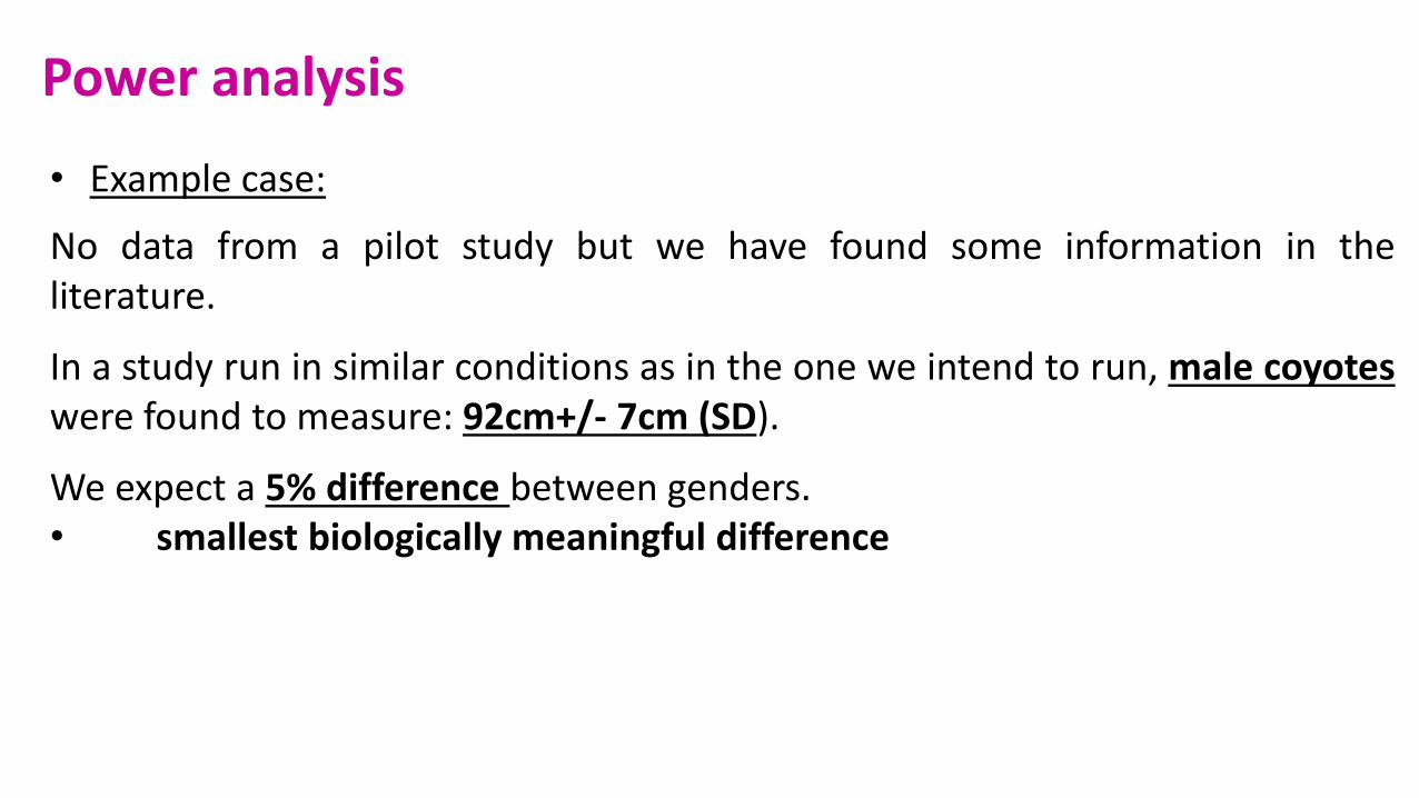
• Example case:
No data from a pilot study but we have found some information in theliterature.
In a study run in similar conditions as in the one we intend to run, male coyoteswere found to measure: 92cm+/- 7cm (SD).
We expect a 5% difference between genders.• smallest biologically meaningful difference
Power analysis
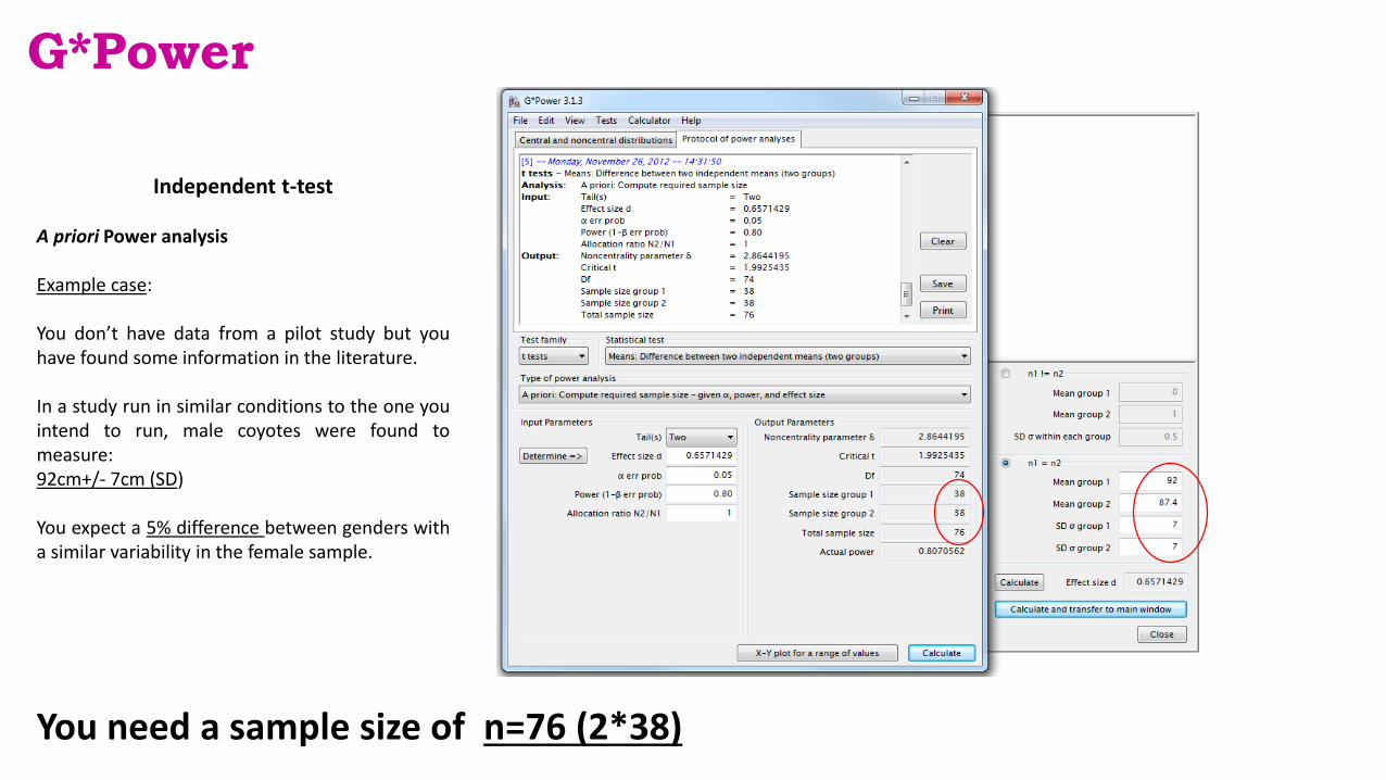
G*Power
Independent t-test
A priori Power analysis
Example case:
You don’t have data from a pilot study but youhave found some information in the literature.
In a study run in similar conditions to the one youintend to run, male coyotes were found tomeasure:92cm+/- 7cm (SD)
You expect a 5% difference between genders witha similar variability in the female sample.
You need a sample size of n=76 (2*38)

Power Analysis
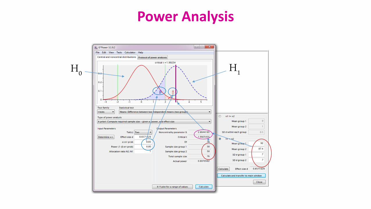
Power Analysis
H0 H1
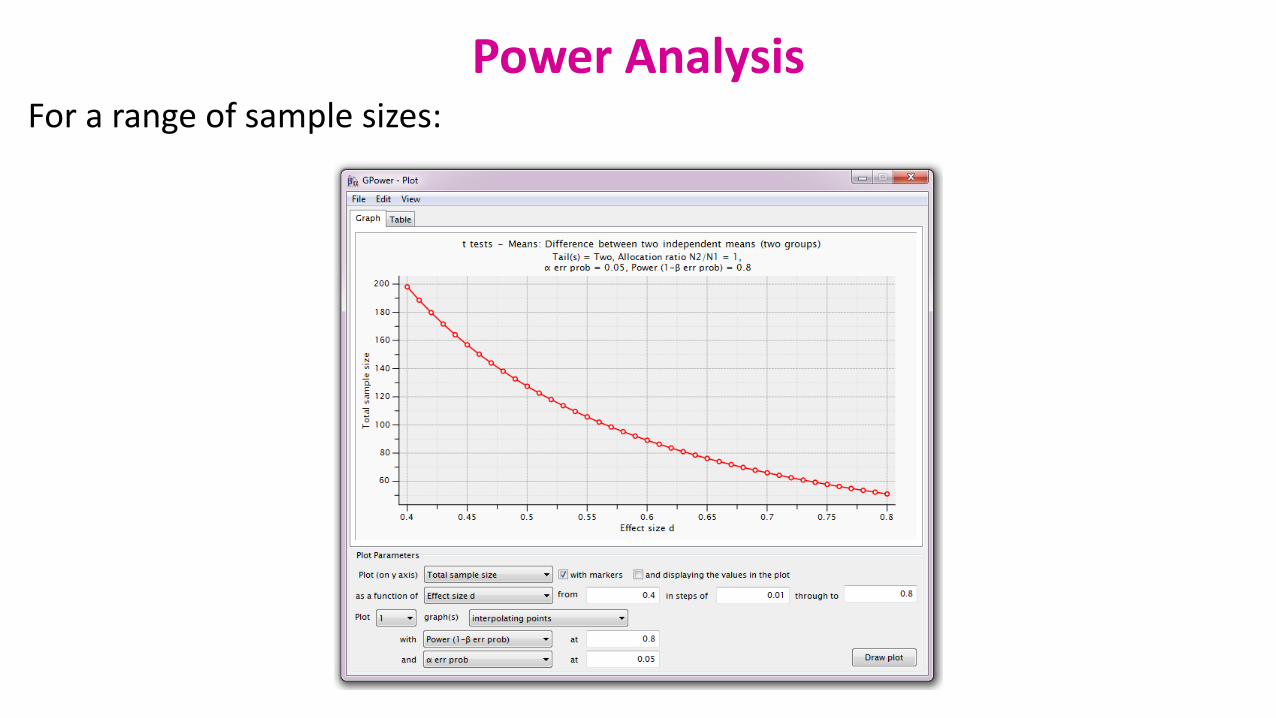
For a range of sample sizes:
Power Analysis

Data exploration ≠ plotting data
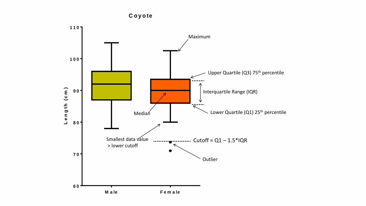
C o y o te
M a le F e m a le
6 0
7 0
8 0
9 0
1 0 0
1 1 0
Le
ng
th
(c
m)
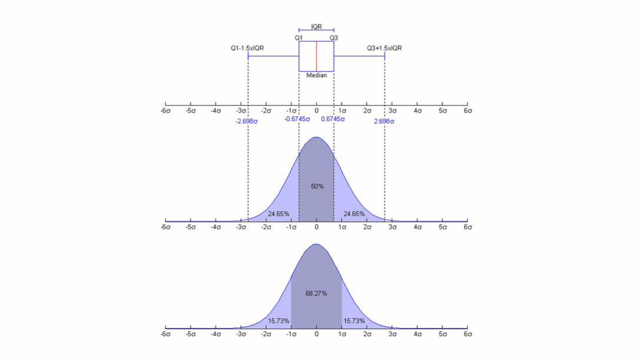
Cutoff = Q1 – 1.5*IQR
Median
Maximum
Smallest data value> lower cutoff
Interquartile Range (IQR)
Lower Quartile (Q1) 25th percentile
Outlier
Upper Quartile (Q3) 75th percentile
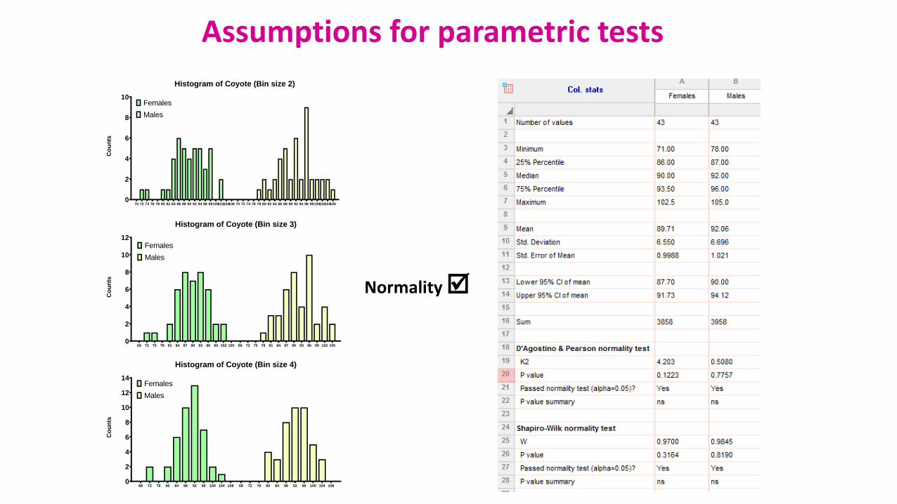
Assumptions for parametric tests
Normality
Histogram of Coyote (Bin size 2)
70 72 74 76 78 80 82 84 86 88 90 92 94 96 98100102104106 70 72 74 76 78 80 82 84 86 88 90 92 94 96 981001021041060
2
4
6
8
10Females
MalesC
ou
nts
Histogram of Coyote (Bin size 3)
69 72 75 78 81 84 87 90 93 96 99 102 105 69 72 75 78 81 84 87 90 93 96 99 102 1050
2
4
6
8
10
12Females
Males
Co
un
ts
Histogram of Coyote (Bin size 4)
68 72 76 80 84 88 92 96 100 104 108 68 72 76 80 84 88 92 96 100 104 1080
2
4
6
8
10
12
14Females
Males
Co
un
ts
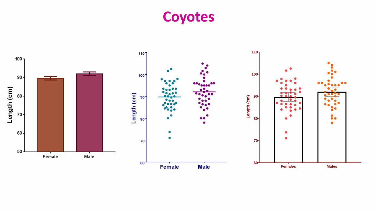
Coyotes
Females Males60
70
80
90
100
110
Len
gth
(cm
)
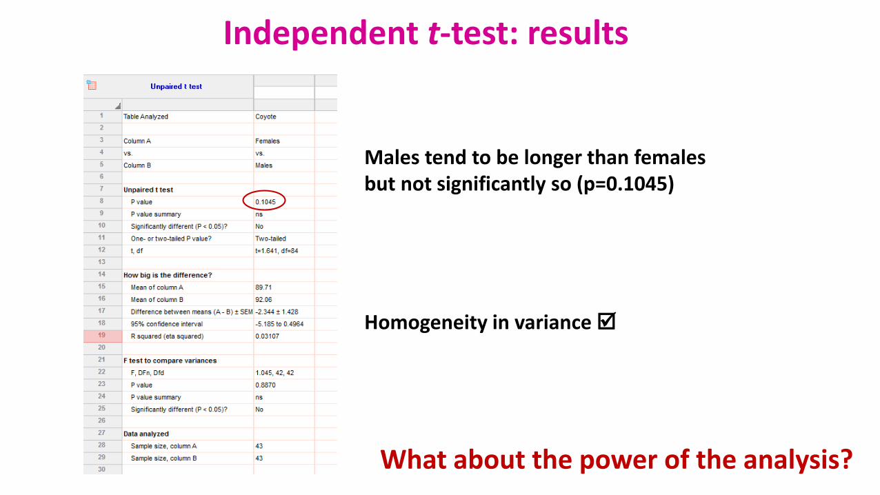
Independent t-test: results
Males tend to be longer than femalesbut not significantly so (p=0.1045)
Homogeneity in variance
What about the power of the analysis?
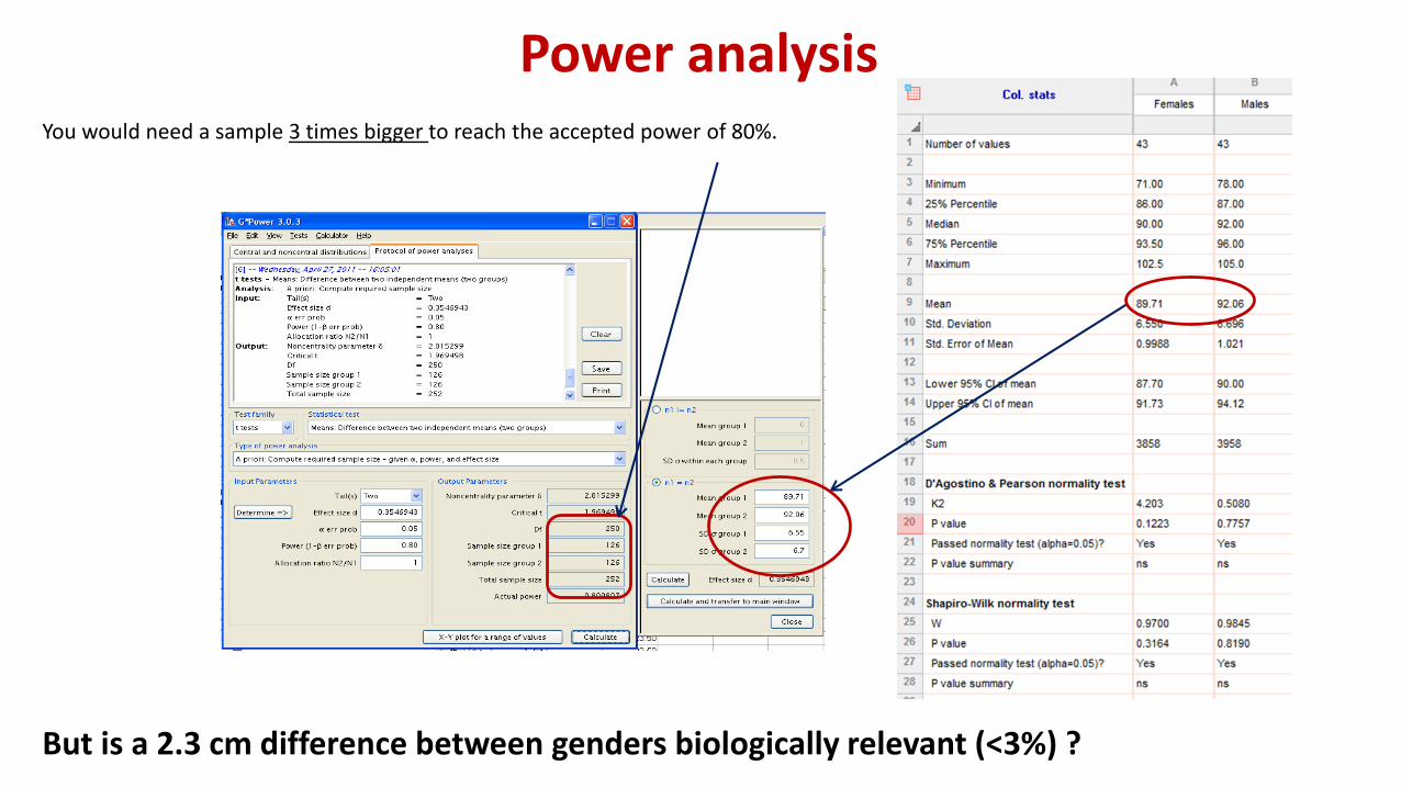
Power analysisYou would need a sample 3 times bigger to reach the accepted power of 80%.
But is a 2.3 cm difference between genders biologically relevant (<3%) ?
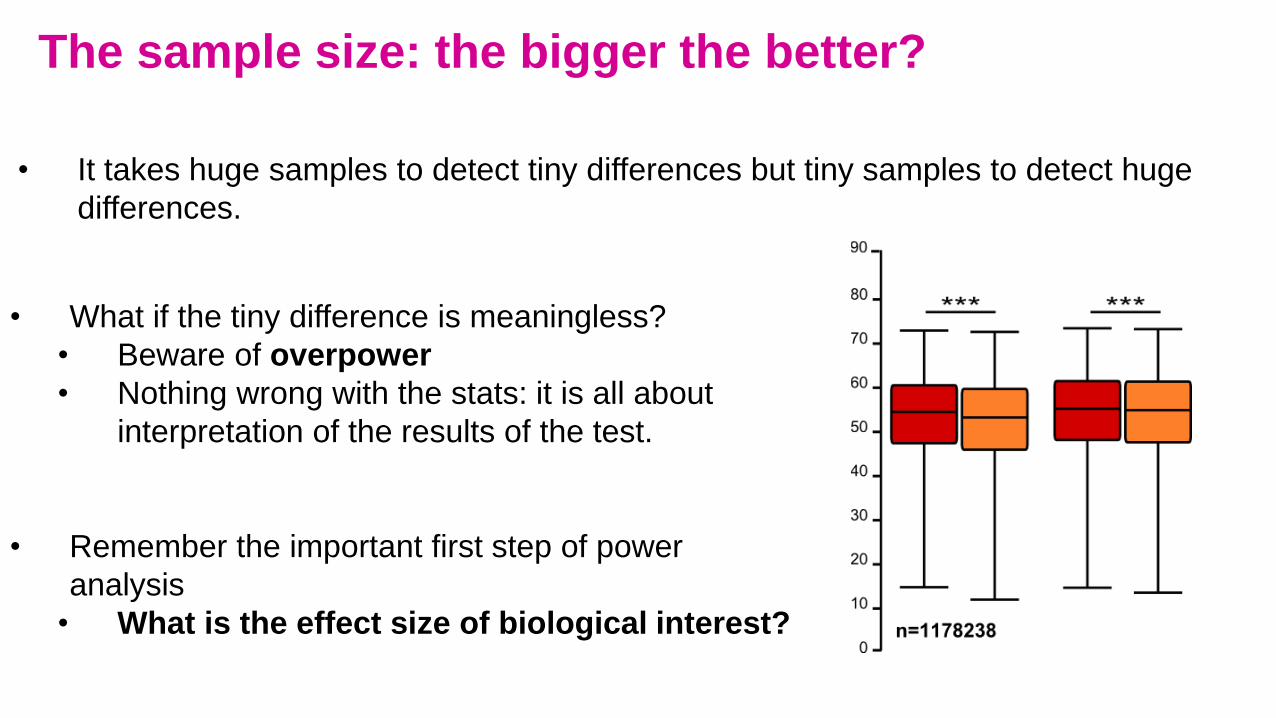
The sample size: the bigger the better?
• What if the tiny difference is meaningless?
• Beware of overpower
• Nothing wrong with the stats: it is all about
interpretation of the results of the test.
• Remember the important first step of power
analysis
• What is the effect size of biological interest?
• It takes huge samples to detect tiny differences but tiny samples to detect huge
differences.
working memory.xlsx
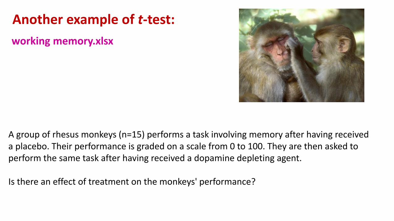
Another example of t-test:
A group of rhesus monkeys (n=15) performs a task involving memory after having received a placebo. Their performance is graded on a scale from 0 to 100. They are then asked to perform the same task after having received a dopamine depleting agent.
Is there an effect of treatment on the monkeys' performance?
working memory.xlsx
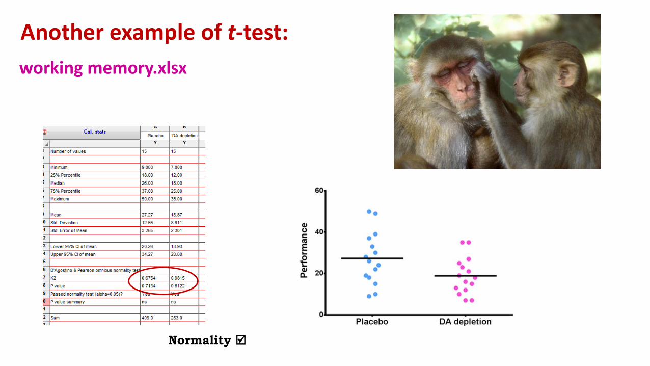
Another example of t-test:
Normality
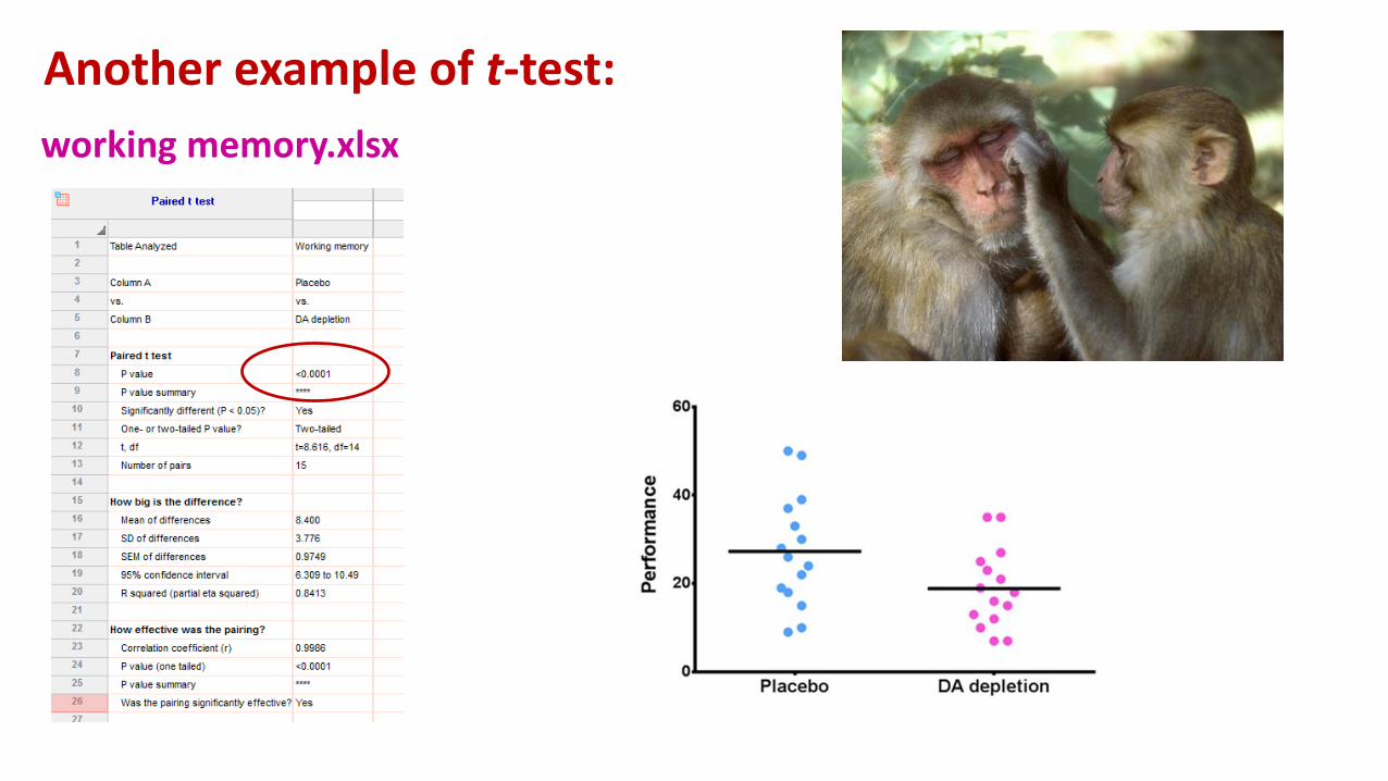
working memory.xlsx
Another example of t-test:
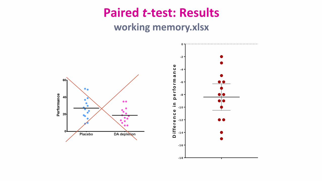
Paired t-test: Resultsworking memory.xlsx
-1 8
-1 6
-1 4
-1 2
-1 0
-8
-6
-4
-2
0
Dif
fere
nc
e i
n p
erfo
rm
an
ce
Comparison of more than 2 means
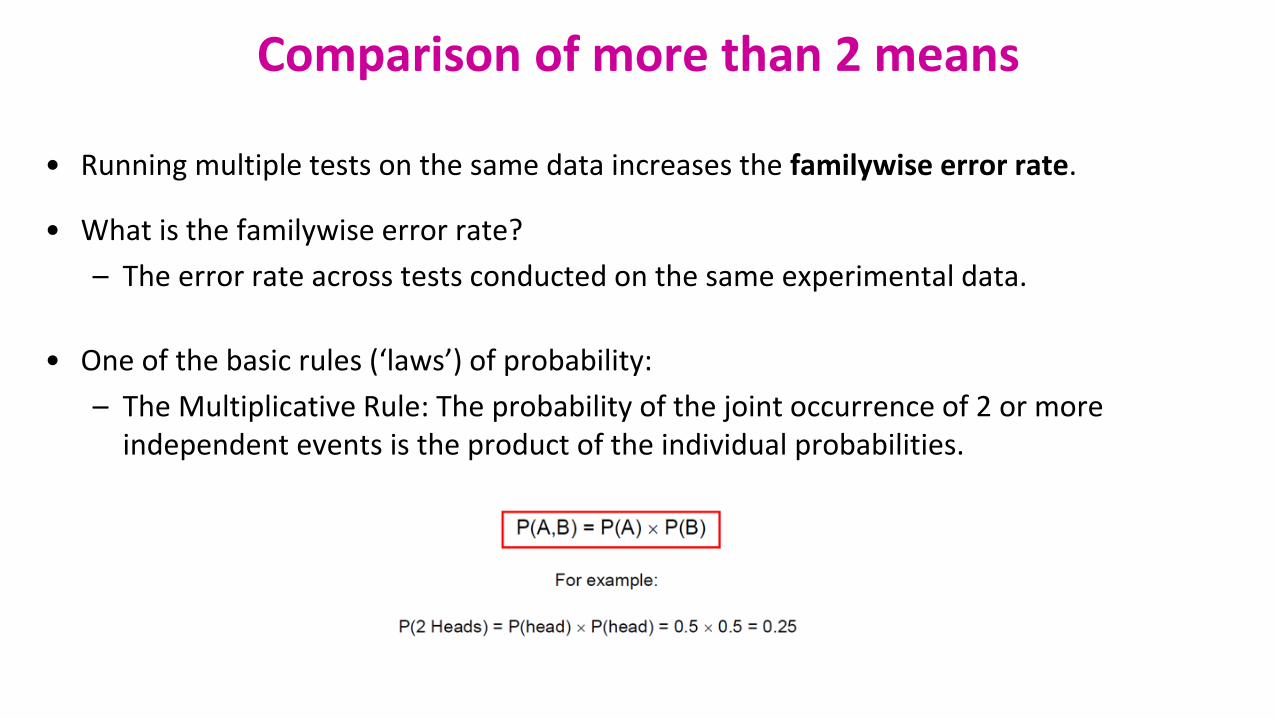
• Running multiple tests on the same data increases the familywise error rate.
• What is the familywise error rate?
– The error rate across tests conducted on the same experimental data.
• One of the basic rules (‘laws’) of probability:
– The Multiplicative Rule: The probability of the joint occurrence of 2 or more independent events is the product of the individual probabilities.
Familywise error rate
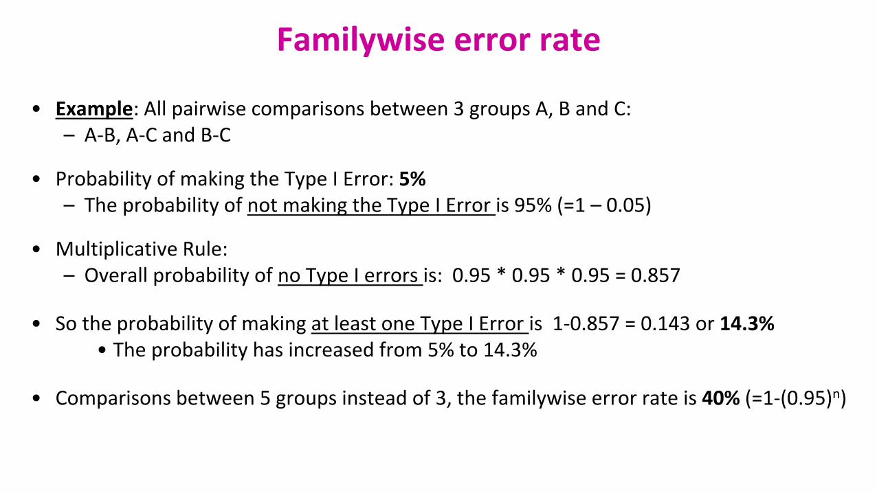
• Example: All pairwise comparisons between 3 groups A, B and C: – A-B, A-C and B-C
• Probability of making the Type I Error: 5%– The probability of not making the Type I Error is 95% (=1 – 0.05)
• Multiplicative Rule:– Overall probability of no Type I errors is: 0.95 * 0.95 * 0.95 = 0.857
• So the probability of making at least one Type I Error is 1-0.857 = 0.143 or 14.3%• The probability has increased from 5% to 14.3%
• Comparisons between 5 groups instead of 3, the familywise error rate is 40% (=1-(0.95)n)
• Solution to the increase of familywise error rate: correction for multiple comparisons– Post-hoc tests
• Many different ways to correct for multiple comparisons:– Different statisticians have designed corrections addressing different issues
• e.g. unbalanced design, heterogeneity of variance, liberal vs conservative
• However, they all have one thing in common: – the more tests, the higher the familywise error rate: the more stringent the correction
• Tukey, Bonferroni, Sidak, Benjamini-Hochberg …– Two ways to address the multiple testing problem
• Familywise Error Rate (FWER) vs. False Discovery Rate (FDR)
Familywise error rate
• FWER: Bonferroni: αadjust = 0.05/n comparisons e.g. 3 comparisons: 0.05/3=0.016– Problem: very conservative leading to loss of power (lots of false negative)– 10 comparisons: threshold for significance: 0.05/10: 0.005– Pairwise comparisons across 20.000 genes
• FDR: Benjamini-Hochberg: the procedure controls the expected proportion of “discoveries” (significant tests) that are false (false positive).– Less stringent control of Type I Error than FWER procedures which control the probability of at least
one Type I Error– More power at the cost of increased numbers of Type I Errors.
• Difference between FWER and FDR: – a p-value of 0.05 implies that 5% of all tests will result in false positives.
– a FDR adjusted p-value (or q-value) of 0.05 implies that 5% of significant tests will result in false positives.
Multiple testing problem
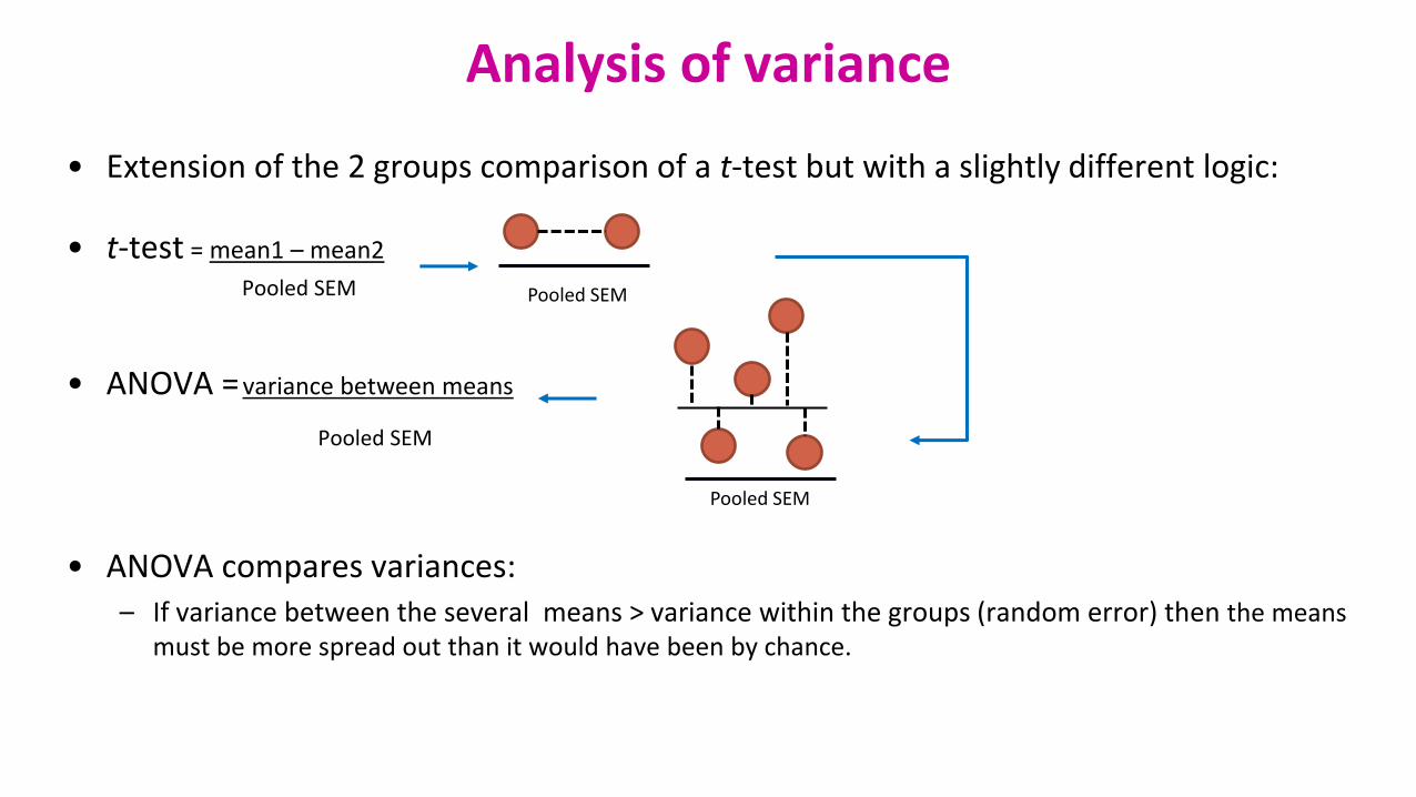
• Extension of the 2 groups comparison of a t-test but with a slightly different logic:
• t-test = mean1 – mean2
Pooled SEM
• ANOVA =variance between means
Pooled SEM
• ANOVA compares variances: – If variance between the several means > variance within the groups (random error) then the means
must be more spread out than it would have been by chance.
Analysis of variance
Pooled SEM
Pooled SEM
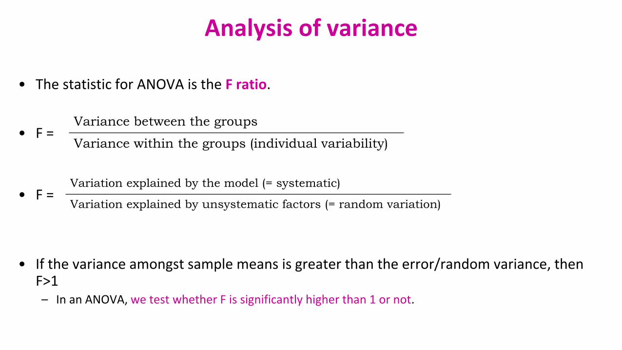
• The statistic for ANOVA is the F ratio.
• F =
• F =
• If the variance amongst sample means is greater than the error/random variance, then F>1– In an ANOVA, we test whether F is significantly higher than 1 or not.
Variance between the groups
Variance within the groups (individual variability)
Variation explained by the model (= systematic)
Variation explained by unsystematic factors (= random variation)
Analysis of variance
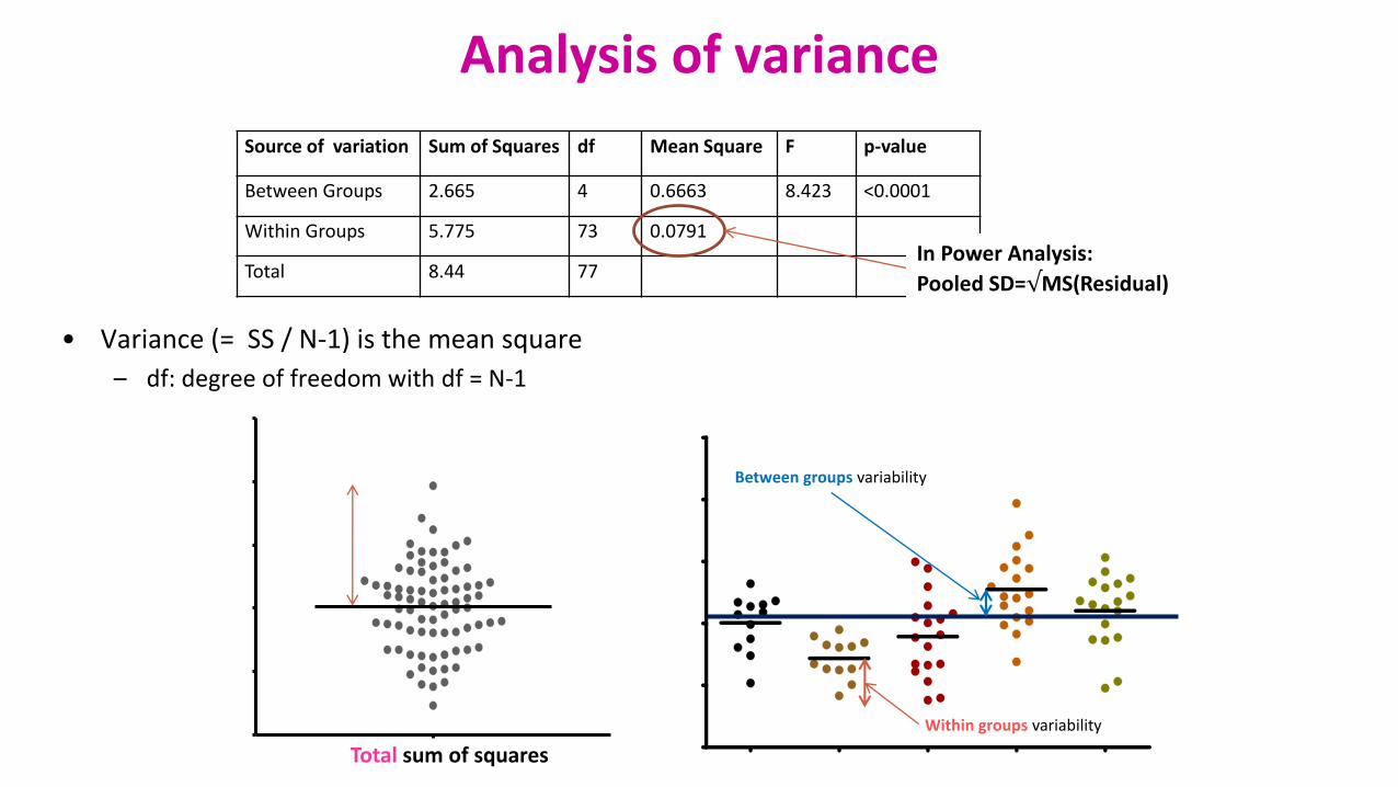
• Variance (= SS / N-1) is the mean square
– df: degree of freedom with df = N-1
Total sum of squares
Between groups variability
Source of variation Sum of Squares df Mean Square F p-value
Between Groups 2.665 4 0.6663 8.423 <0.0001
Within Groups 5.775 73 0.0791
Total 8.44 77
Within groups variability
In Power Analysis:
Pooled SD=√MS(Residual)
Analysis of variance
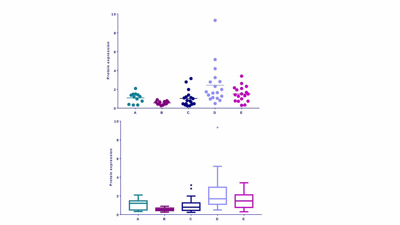
Example: protein.expression.csv
• Question: is there a difference in protein expression between the 5 cell lines?
• 1 Plot the data
• 2 Check the assumptions for parametric test
• 3 Statistical analysis: ANOVA
A B C D E
0
2
4
6
8
1 0
Pro
tein
ex
pre
ss
ion
A B C D E
0
2
4
6
8
1 0
Pro
tein
ex
pre
ss
ion
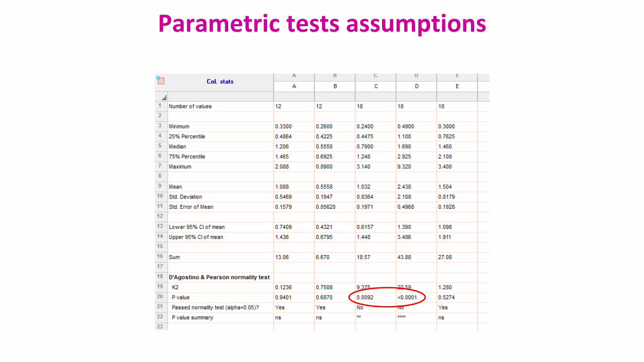
Parametric tests assumptions
A B C D E
0 .1
1
1 0
Pro
tein
ex
pre
ss
ion
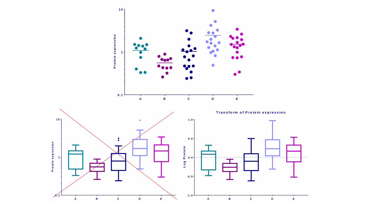
A B C D E
0 .1
1
1 0
Pro
tein
ex
pre
ss
ion
A B C D E
-1 .0
-0 .5
0 .0
0 .5
1 .0
T ra n s fo rm o f P r o te in e x p re s s io n
Lo
g P
ro
tein
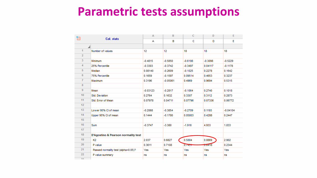
Parametric tests assumptions
Analysis of variance: Post hoc tests
• The ANOVA is an “omnibus” test: it tells you that there is (or not) a difference between your means but not exactly which means are significantly different from which other ones.
– To find out, you need to apply post hoc tests.
– These post hoc tests should only be used when the ANOVA finds a significant effect.
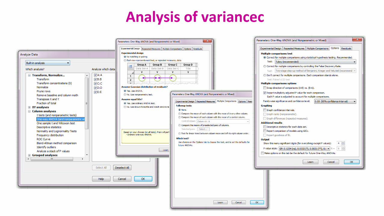
Analysis of variancec
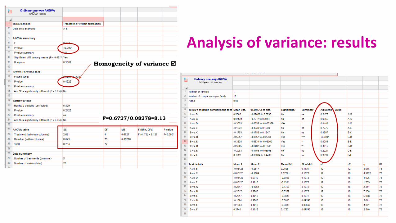
Analysis of variance: resultsHomogeneity of variance
F=0.6727/0.08278=8.13
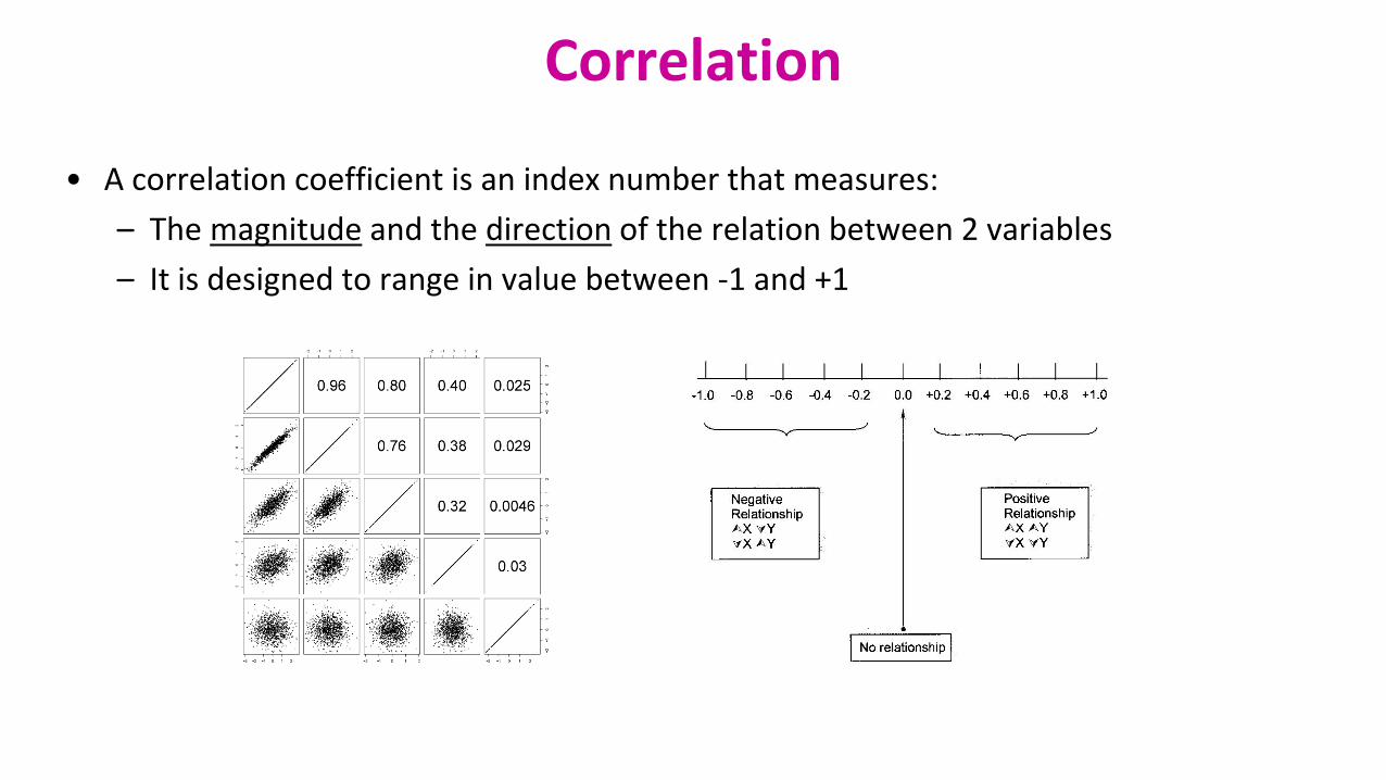
• A correlation coefficient is an index number that measures:
– The magnitude and the direction of the relation between 2 variables
– It is designed to range in value between -1 and +1
Correlation
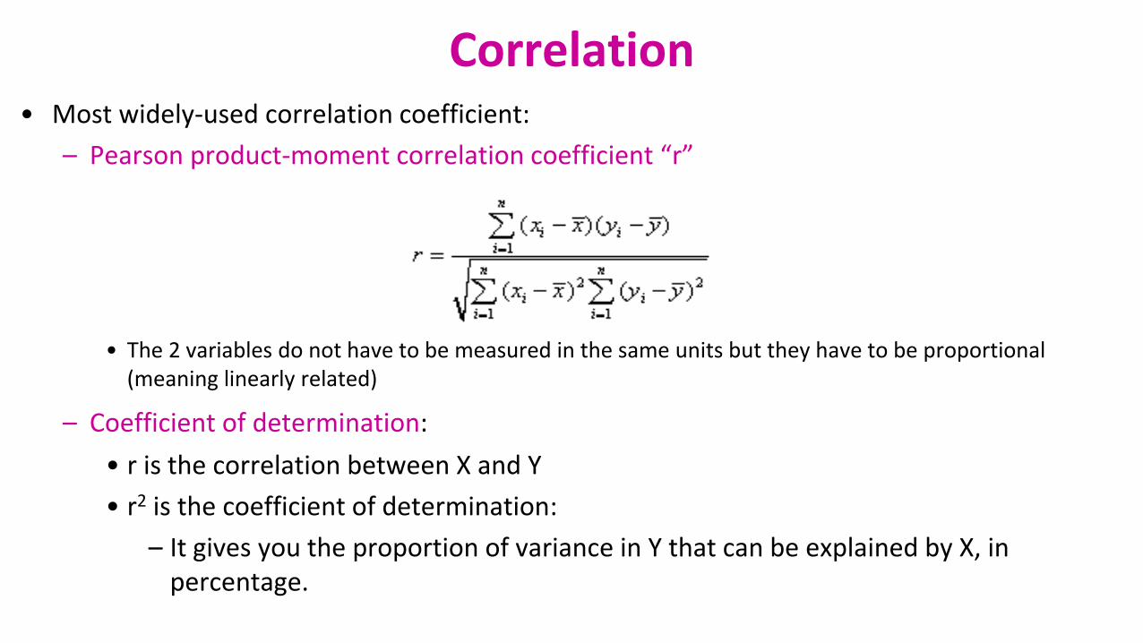
Correlation• Most widely-used correlation coefficient:
– Pearson product-moment correlation coefficient “r”
• The 2 variables do not have to be measured in the same units but they have to be proportional (meaning linearly related)
– Coefficient of determination:
• r is the correlation between X and Y
• r2 is the coefficient of determination:
– It gives you the proportion of variance in Y that can be explained by X, in percentage.
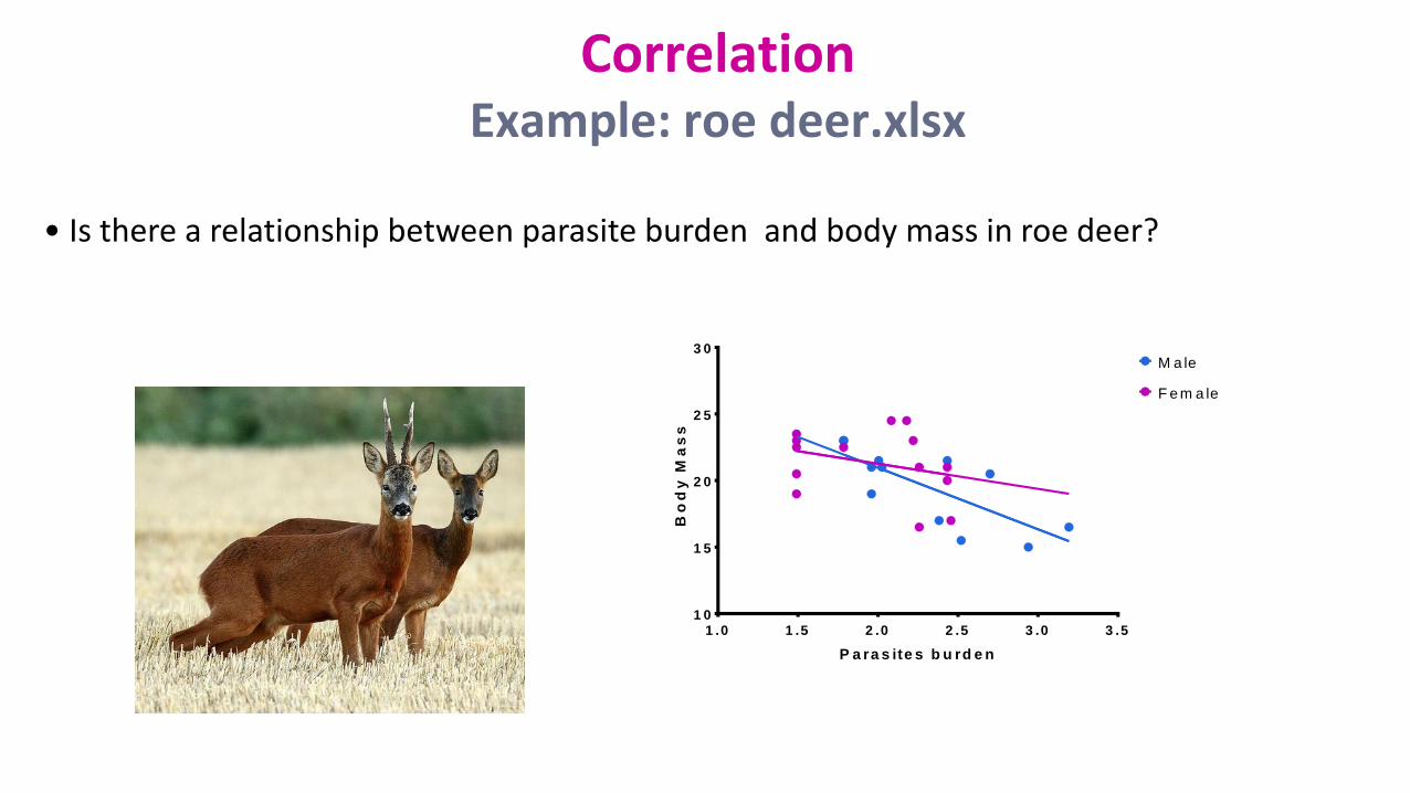
• Is there a relationship between parasite burden and body mass in roe deer?
1 .0 1 .5 2 .0 2 .5 3 .0 3 .51 0
1 5
2 0
2 5
3 0M a le
F e m a le
P a ra s ite s b u rd e n
Bo
dy
Ma
ss
CorrelationExample: roe deer.xlsx
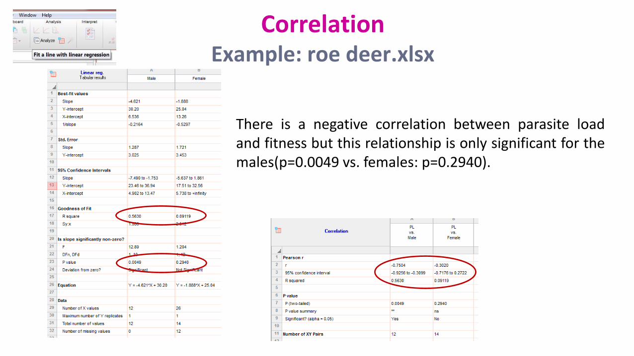
CorrelationExample: roe deer.xlsx
There is a negative correlation between parasite loadand fitness but this relationship is only significant for themales(p=0.0049 vs. females: p=0.2940).
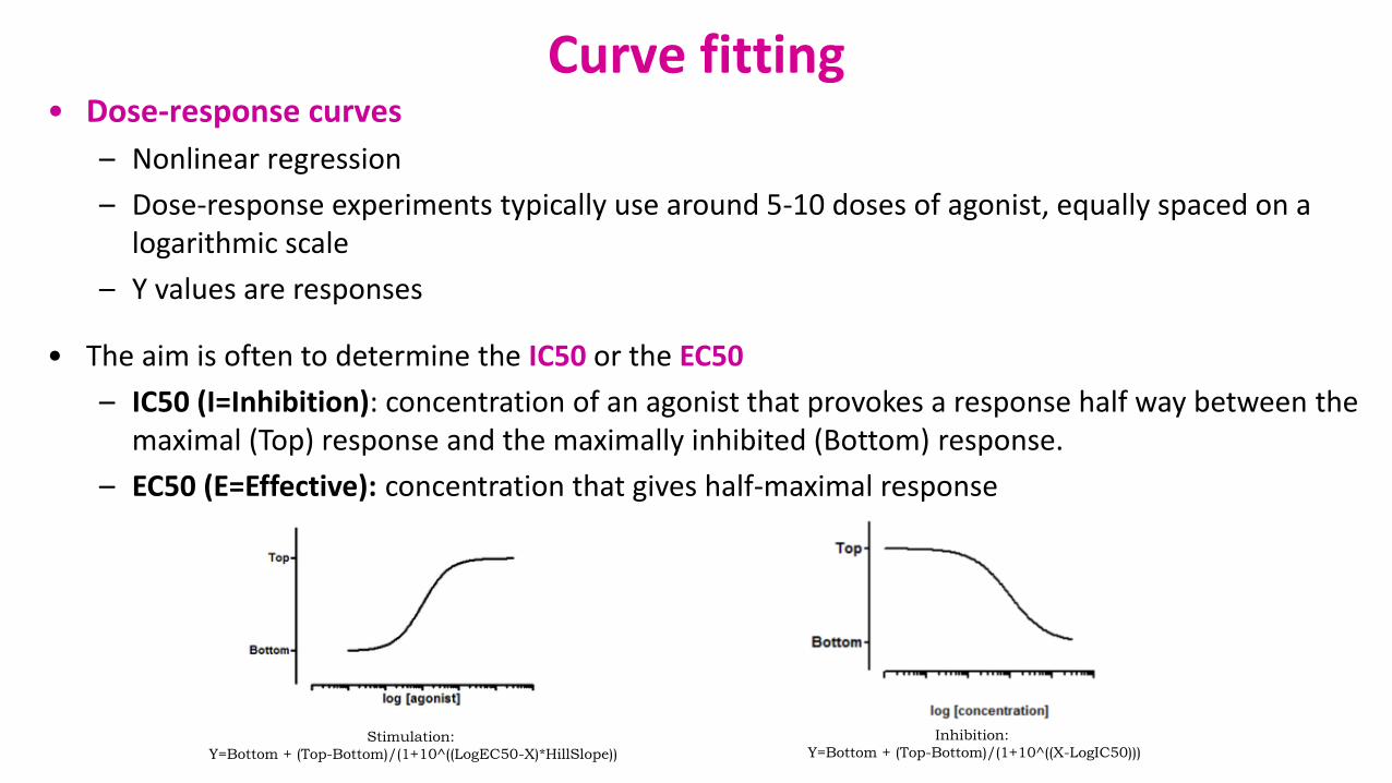
Curve fitting• Dose-response curves
– Nonlinear regression
– Dose-response experiments typically use around 5-10 doses of agonist, equally spaced on a logarithmic scale
– Y values are responses
• The aim is often to determine the IC50 or the EC50
– IC50 (I=Inhibition): concentration of an agonist that provokes a response half way between the maximal (Top) response and the maximally inhibited (Bottom) response.
– EC50 (E=Effective): concentration that gives half-maximal response
Stimulation:
Y=Bottom + (Top-Bottom)/(1+10^((LogEC50-X)*HillSlope))
Inhibition:
Y=Bottom + (Top-Bottom)/(1+10^((X-LogIC50)))
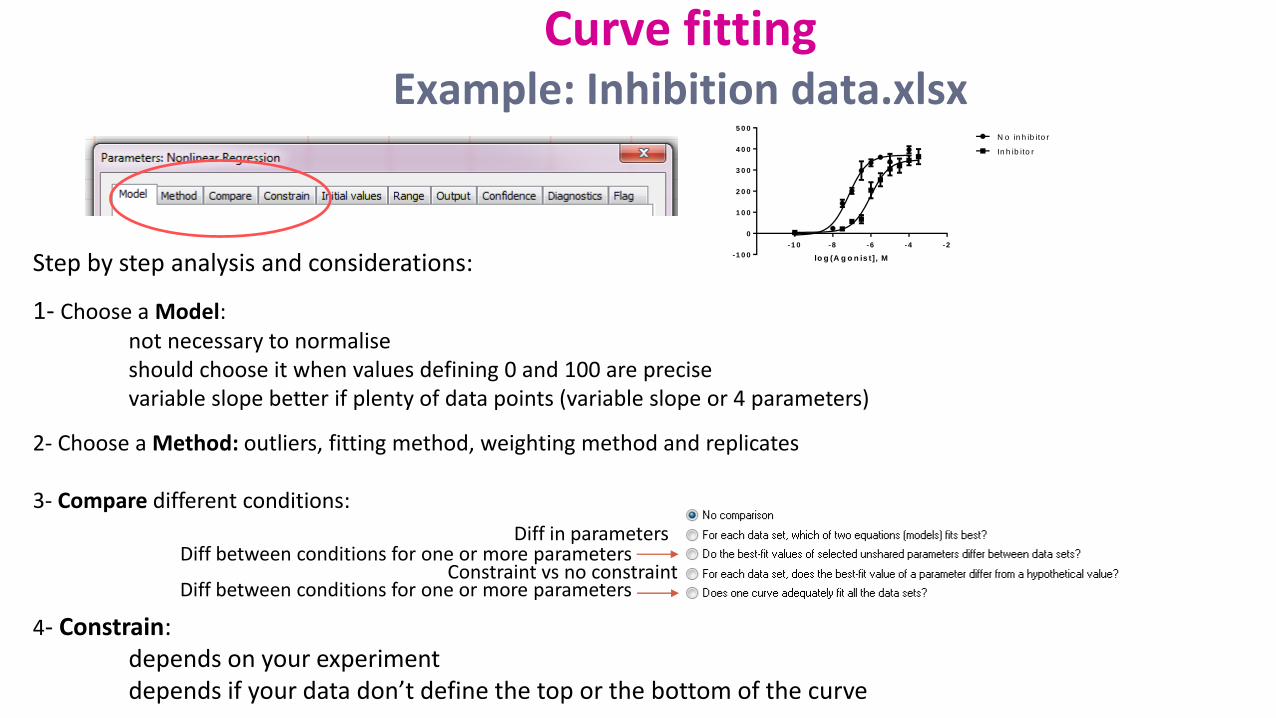
Step by step analysis and considerations:
1- Choose a Model:not necessary to normaliseshould choose it when values defining 0 and 100 are precisevariable slope better if plenty of data points (variable slope or 4 parameters)
2- Choose a Method: outliers, fitting method, weighting method and replicates
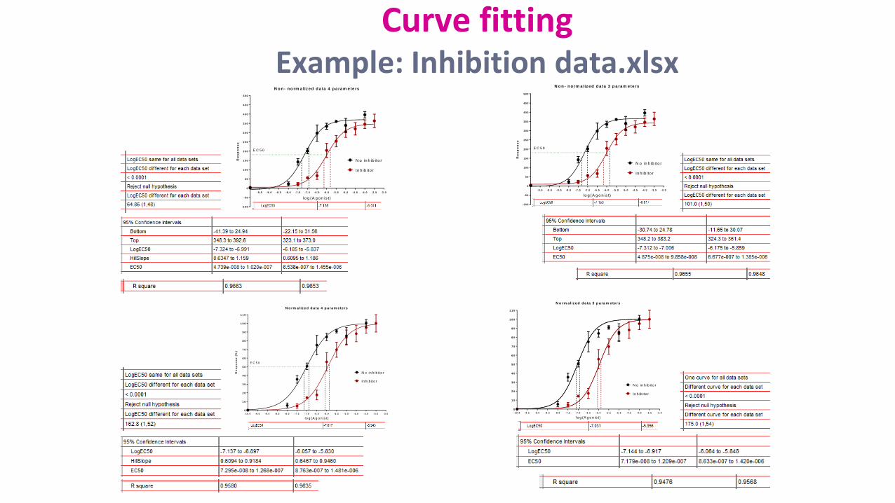
3- Compare different conditions:
4- Constrain:depends on your experimentdepends if your data don’t define the top or the bottom of the curve
Diff in parameters
Constraint vs no constraintDiff between conditions for one or more parameters
Diff between conditions for one or more parameters
-1 0 -8 -6 -4 -2
-1 0 0
0
1 0 0
2 0 0
3 0 0
4 0 0
5 0 0
lo g (A g o n is t], M
N o in h ib ito r
In h ib ito r
Curve fittingExample: Inhibition data.xlsx
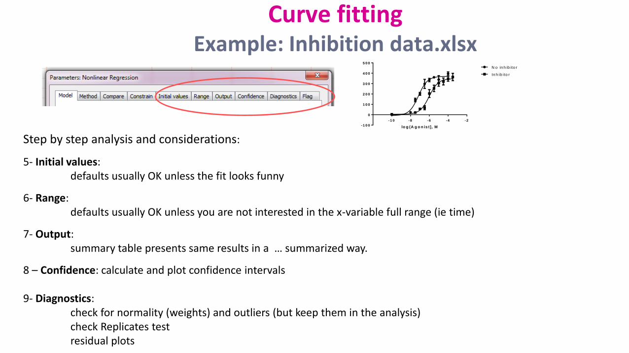
Step by step analysis and considerations:
5- Initial values:defaults usually OK unless the fit looks funny
6- Range:defaults usually OK unless you are not interested in the x-variable full range (ie time)
7- Output:summary table presents same results in a … summarized way.
8 – Confidence: calculate and plot confidence intervals
9- Diagnostics:check for normality (weights) and outliers (but keep them in the analysis) check Replicates testresidual plots
-1 0 -8 -6 -4 -2
-1 0 0
0
1 0 0
2 0 0
3 0 0
4 0 0
5 0 0
lo g (A g o n is t], M
N o in h ib ito r
In h ib ito r
Curve fittingExample: Inhibition data.xlsx
-9 .5 -9 .0 -8 .5 -8 .0 -7 .5 -7 .0 -6 .5 -6 .0 -5 .5 -5 .0 -4 .5 -4 .0 -3 .5 -3 .0
-1 0 0
-5 0
0
5 0
1 0 0
1 5 0
2 0 0
2 5 0
3 0 0
3 5 0
4 0 0
4 5 0
5 0 0
N o n - n o rm a liz e d d a ta 4 p a ra m e te rs
lo g (A g o n is t)
Re
sp
on
se
N o in h ib ito r
In h ib ito r
E C 5 0
-9 .5 -9 .0 -8 .5 -8 .0 -7 .5 -7 .0 -6 .5 -6 .0 -5 .5 -5 .0 -4 .5 -4 .0 -3 .5 -3 .0
-1 0 0
-5 0
0
5 0
1 0 0
1 5 0
2 0 0
2 5 0
3 0 0
3 5 0
4 0 0
4 5 0
5 0 0
N o n - n o rm a liz e d d a ta 3 p a ra m e te rs
lo g (A g o n is t)
Re
sp
on
se
N o in h ib ito r
In h ib ito r
E C 5 0
-1 0 .0 -9 .5 -9 .0 -8 .5 -8 .0 -7 .5 -7 .0 -6 .5 -6 .0 -5 .5 -5 .0 -4 .5 -4 .0 -3 .5 -3 .0
0
1 0
2 0
3 0
4 0
5 0
6 0
7 0
8 0
9 0
1 0 0
1 1 0
N o rm a liz e d d a ta 4 p a ra m e te rs
lo g (A g o n is t)
Re
sp
on
se
(%
)
N o in h ib ito r
In h ib ito r
E C 5 0
-1 0 .0 -9 .5 -9 .0 -8 .5 -8 .0 -7 .5 -7 .0 -6 .5 -6 .0 -5 .5 -5 .0 -4 .5 -4 .0 -3 .5 -3 .0
0
1 0
2 0
3 0
4 0
5 0
6 0
7 0
8 0
9 0
1 0 0
1 1 0
N o rm a liz e d d a ta 3 p a ra m e te rs
lo g (A g o n is t)
N o in h ib ito r
In h ib ito r
Curve fittingExample: Inhibition data.xlsx
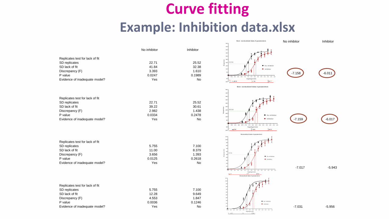
Replicates test for lack of fit
SD replicates 22.71 25.52
SD lack of fit 41.84 32.38
Discrepancy (F) 3.393 1.610
P value 0.0247 0.1989
Evidence of inadequate model? Yes No
Replicates test for lack of fit
SD replicates 22.71 25.52
SD lack of fit 39.22 30.61
Discrepancy (F) 2.982 1.438
P value 0.0334 0.2478
Evidence of inadequate model? Yes No
Replicates test for lack of fit
SD replicates 5.755 7.100
SD lack of fit 11.00 8.379
Discrepancy (F) 3.656 1.393
P value 0.0125 0.2618
Evidence of inadequate model? Yes No
Replicates test for lack of fit
SD replicates 5.755 7.100
SD lack of fit 12.28 9.649
Discrepancy (F) 4.553 1.847
P value 0.0036 0.1246
Evidence of inadequate model? Yes No
-1 0 .0 -9 .5 -9 .0 -8 .5 -8 .0 -7 .5 -7 .0 -6 .5 -6 .0 -5 .5 -5 .0 -4 .5 -4 .0 -3 .5 -3 .0
0
1 0
2 0
3 0
4 0
5 0
6 0
7 0
8 0
9 0
1 0 0
1 1 0
N o rm a liz e d d a ta 4 p a ra m e te rs
lo g (A g o n is t)
Re
sp
on
se
(%
)
N o in h ib ito r
In h ib ito r
E C 5 0
-1 0 .0 -9 .5 -9 .0 -8 .5 -8 .0 -7 .5 -7 .0 -6 .5 -6 .0 -5 .5 -5 .0 -4 .5 -4 .0 -3 .5 -3 .0
0
1 0
2 0
3 0
4 0
5 0
6 0
7 0
8 0
9 0
1 0 0
1 1 0
N o rm a liz e d d a ta 3 p a ra m e te rs
lo g (A g o n is t)
N o in h ib ito r
In h ib ito r
No inhibitor Inhibitor
-7.031 -5.956
-7.158 -6.011
-7.159 -6.017
-7.017 -5.943
No inhibitor Inhibitor
-9 .5 -9 .0 -8 .5 -8 .0 -7 .5 -7 .0 -6 .5 -6 .0 -5 .5 -5 .0 -4 .5 -4 .0 -3 .5 -3 .0
-1 0 0
-5 0
0
5 0
1 0 0
1 5 0
2 0 0
2 5 0
3 0 0
3 5 0
4 0 0
4 5 0
5 0 0
N o n - n o rm a liz e d d a ta 4 p a ra m e te rs
lo g (A g o n is t)
Re
sp
on
se
N o in h ib ito r
In h ib ito r
E C 5 0
-9 .5 -9 .0 -8 .5 -8 .0 -7 .5 -7 .0 -6 .5 -6 .0 -5 .5 -5 .0 -4 .5 -4 .0 -3 .5 -3 .0
-1 0 0
-5 0
0
5 0
1 0 0
1 5 0
2 0 0
2 5 0
3 0 0
3 5 0
4 0 0
4 5 0
5 0 0
N o n - n o rm a liz e d d a ta 3 p a ra m e te rs
lo g (A g o n is t)
Re
sp
on
se
N o in h ib ito r
In h ib ito r
E C 5 0
Curve fittingExample: Inhibition data.xlsx