Embed Size (px)
Citation preview

Introduction to Statistics
Dr Linda Morgan
Clinical Chemistry Division
School of Clinical Laboratory Sciences
Outline
• Types of data• Descriptive statistics• Estimates and confidence intervals• Hypothesis testing• Comparing groups• Relation between variables• Statistical aspects of study design• Pitfalls

Types of data
• Categorical data– Ordered categorical data
• Numerical data– Discrete– Continuous

Descriptive statisticsCategorical variables
• Graphical representation – bar diagram
• Numbers and proportions in each category
smoking habit
heavy smokerlight smokerex-smokernon-smoker
Pe
rce
nt
50
40
30
20
10
0

Descriptive statisticsContinuous variables
• Distributions– Gaussian– Lognormal– Non-parametric
• Central tendency– Mean– Median
• Scatter– Standard deviation– Range– Interquartile range

Maternal age
42.5
40.0
37.5
35.0
32.5
30.0
27.5
25.0
22.5
20.0
17.5
15.0
60
50
40
30
20
10
0
Std. Dev = 4.84
Mean = 28.0
N = 223.00
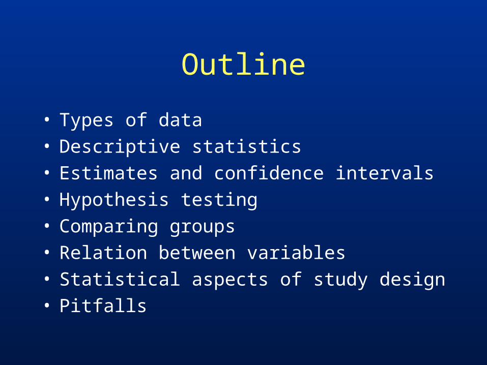
Gaussian (normal) distribution
• Central tendency
Mean = x
n
• Scatter
Variance = (x-mean)2
n –1
Standard deviation = variance
Gaussian (normal) distribution

Plasma renin concentration
36.0
34.0
32.0
30.0
28.0
26.0
24.0
22.0
20.0
18.0
16.0
14.0
12.0
10.0
8.0
6.0
4.0
2.0
20
10
0
Std. Dev = 5.36
Mean = 9.3
N = 73.00
Lognormal distribution

Log plasma renin concentration
1.501.381.251.131.00.88.75.63.50.38
30
20
10
0
Std. Dev = .21
Mean = .91
N = 73.00
Lognormal distribution

Lognormal distribution
• Mean = log x n
• Geometric mean = antilog of mean (10mean)
• Median– Rank data in order– Median = (n+1) / 2th observation

Variability
• Variance = (x-mean)2
n –1
• Standard deviation = variance
• Range
• Interquartile range
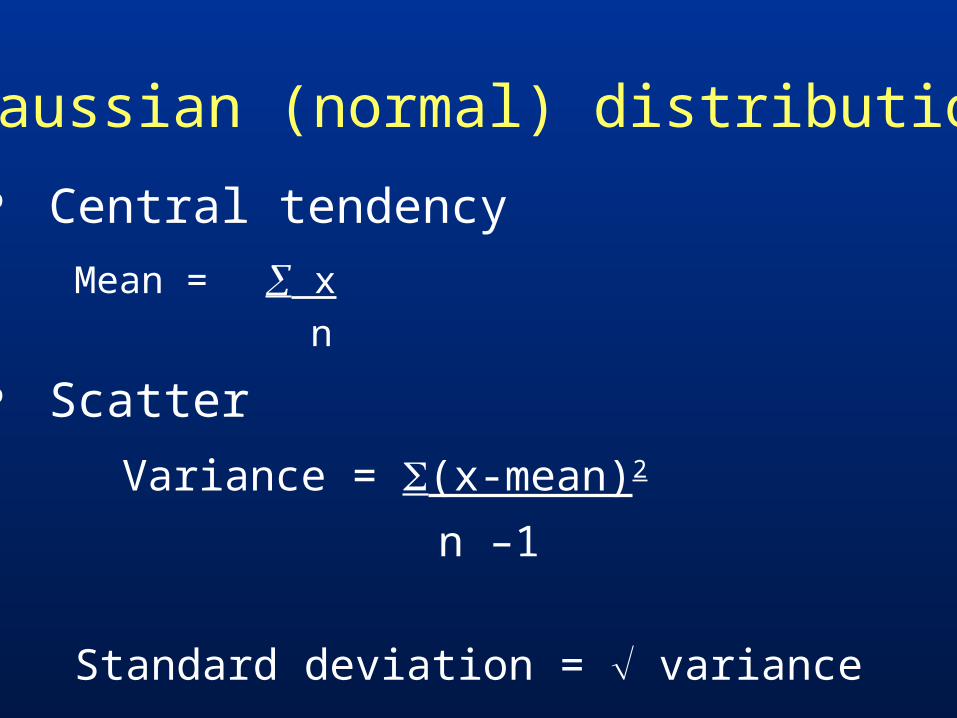
Variability of Sample Mean
• The sample mean is an estimate of the population mean
• The standard error of the mean describes the distribution of the sample mean
• Estimated SEM = SD/ n• The distribution of the sample mean is
Normal providing n is large

Standard error of the difference between two means• SEM = SD/ n• Variance of the mean = SD2/n• Variance of the difference between two
sample means
= sum of the variances of the two means= (SD2/n)1 + (SD2/n)2
• SE of difference between means
= [(SD2/n)1 + (SD2/n)2 ]

Variability of a sample proportion
• Assume Normal distribution when np and n(1-p) are > 5
• SE of a Binomial proportion =
(pq/n) where q = 1-p

Standard error of the difference between two
proportions• SE (p1 – p2 )
= [variance (p1) + variance (p2) ]
= [ (p1 q1 /n1) + (p2 q2 /n2) ]

Confidence intervals of means
• 95% ci for the mean =
Sample mean 1.96 SEM
• 95% ci for difference between 2 means =
(mean1 – mean2 ) 1.96 SE of difference

Confidence intervals of proportions
• 95% ci for proportion
= p 1.96 (pq/n)
• 95% ci for difference between two proportions
= (p1 – p2 ) 1.96 x SE (p1 – p2 )

Hypothesis testing
• The null hypothesis
• The alternative hypothesis
• What is a P value?

Comparing 2 groups of continuous data
• Normal distribution:
paired or unpaired t test
• Non-Normal distribution:
transform data
OR
Mann-Whitney-Wilcoxon test

Paired t test
We wish to compare the fasting blood cholesterol levels in 10 subjects before and after treatment with a new drug.
What is the null hypothesis?

Paired t testSubject Fasting cholesterol DNumber Predrug Postdrug01 6.7 4.4 2.302 7.8 7.0 0.803 8.1 6.0 2.104 5.5 5.8 -0.305 8.6 9.0 -0.406 6.7 6.1 0.607 7.1 7.3 -0.208 9.9 9.9 009 8.2 6.3 1.910 6.5 7.1 -0.6

Paired t test
• Calculate the mean and SEM of D
• The null hypothesis is that D = 0
• The test statistic t =
mean(d) – 0
SEM (d)

Paired t test
• Mean = 0.62• SEM = 0.351• t = 1.766• Degrees of freedom = n - 1 = 9• From tables of t,
2-tailed probability (P) is between 0.1 and 0.2• How would you interpret this?

Comparing 2 groups of categorical data
• In a study of the effect of smoking on the risk of developing ischaemic heart disease, 250 men with IHD and 250 age-matched healthy controls were asked about their current smoking habits.
• What is the null hypothesis?

Results
• 70 of the 250 patients were smokers
• 30 of the healthy controls were smokers
Smoker Non-smoker
Total
IHD 70 180 250
Control 30 220 250
Total 100 400 500

Smoker Non-smoker Total
IHD 70
50
180
200
250
Control 30
50
220
200
250
Total 100 400 500
Calculate expected values, E, for each cell
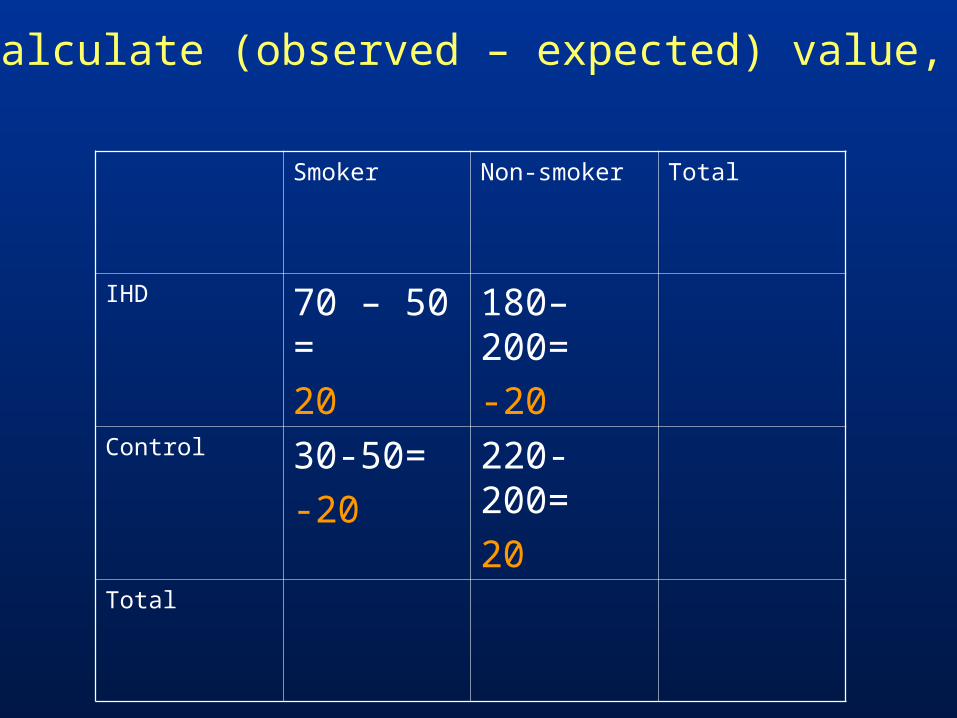
Calculate (observed – expected) value, D
Smoker Non-smoker Total
IHD 70 – 50 =
20
180–200=
-20
Control 30-50=
-20
220-200=
20
Total

Calculate D2/E
Smoker Non-smoker Total
IHD 400/50=
8
400/200=
2
Control 400/50=
8
400/200=
2
Total

Calculate the sum of D2/E
8 + 8 + 2 + 2 = 20
This is the test statistic, chi squaredCompare with tables of chi squared with (r-1)(c-1) degrees of freedom In this case, chi squared with 1 df has a P value of < 0.001
How do you interpret this?

Statistical analysis using computer software
SPSS as an example

Planning
• Experimental design
• Suitable controls
• Database design

Statistical power
• The power of a study to detect an effect depends on:– The size of the effect– The sample size
• The probability of failing to detect an effect where one exists is called
• The power of a study is 100(1-)%• Wide confidence intervals indicate low
statistical power
Statistical power
• The necessary sample size to detect the effect of interest should be calculated in advance
• Pilot data are usually required for these calculations

Statistical power - example
• 30% of the population are carriers of a genetic variant. You wish to test whether this variant increases the risk of Alzheimers Disease.
• For P < 0.05, and 80% power, number of controls and cases required:
Control carriers Case carriers Sample size 30% 50% 10030% 40% 35030% 35% 1400

Multiple testingNumber of Probability of Tests false positive
1 0.052 0.103 0.144 0.195 0.2310 0.4020 0.64
Bonferroni correction: Divide 0.05 by the number of tests to provide the required P value for hypothesis testing at the conventional level of statistical significance

Data trawling
• Decide in advance which statistical tests are to be performed
• Post hoc testing of subgroups should be viewed with caution
• Multiple correlations should be avoided

HELP!
• “In house” support
• Cripps Computing Centre
• Trent Institute for Health Service Research
• Practical Statistics for Medical Research
Douglas G Altman