Introduction to StatisticsIntroduction to Statistics

CorrelationCorrelationChapter 15Chapter 15

April 23-28, 2009April 23-28, 2009Classes #27-28Classes #27-28

CorrelationCorrelation

A statistical technique that is used to A statistical technique that is used to measure and describe a relationship measure and describe a relationship between two variablesbetween two variables– For example: For example:

GPA and TD’s scoredGPA and TD’s scored

Statistics exam scores and amount of time spent Statistics exam scores and amount of time spent studyingstudying

NotationNotation

A correlation requires two scores for each A correlation requires two scores for each individual individual – One score from each of the two variablesOne score from each of the two variables– They are normally identified as X and YThey are normally identified as X and Y

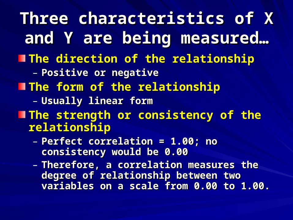
Three characteristics of X and Y Three characteristics of X and Y are being measured…are being measured…

The direction of the relationshipThe direction of the relationship– Positive or negativePositive or negative

The form of the relationshipThe form of the relationship– Usually linear formUsually linear form

The strength or consistency of the The strength or consistency of the relationshiprelationship– Perfect correlation = 1.00; no consistency would Perfect correlation = 1.00; no consistency would

be 0.00be 0.00– Therefore, a correlation measures the degree of Therefore, a correlation measures the degree of

relationship between two variables on a scale relationship between two variables on a scale from 0.00 to 1.00.from 0.00 to 1.00.

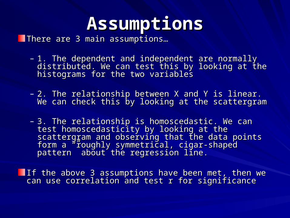
AssumptionsAssumptionsThere are 3 main assumptions…There are 3 main assumptions…

– 1. The dependent and independent are normally 1. The dependent and independent are normally distributed. We can test this by looking at the histograms distributed. We can test this by looking at the histograms for the two variablesfor the two variables

– 2. The relationship between X and Y is linear. We can 2. The relationship between X and Y is linear. We can check this by looking at the scattergramcheck this by looking at the scattergram

– 3. The relationship is homoscedastic. We can test 3. The relationship is homoscedastic. We can test homoscedasticity by looking at the scattergram and homoscedasticity by looking at the scattergram and observing that the data points form a “roughly symmetrical, observing that the data points form a “roughly symmetrical, cigar-shaped pattern” about the regression line.cigar-shaped pattern” about the regression line.

If the above 3 assumptions have been met, then we can use If the above 3 assumptions have been met, then we can use correlation and test r for significancecorrelation and test r for significance

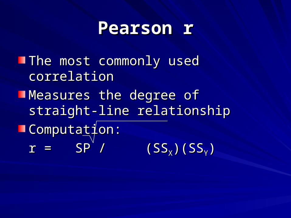
Pearson rPearson r

The most commonly used correlationThe most commonly used correlation

Measures the degree of straight-line Measures the degree of straight-line relationshiprelationship

Computation:Computation:

r = SP / (SSr = SP / (SSXX)(SS)(SSYY))

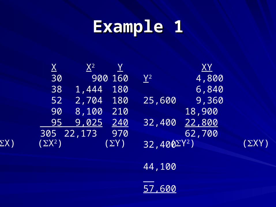
Example 1Example 1

X 30 38 52 90 95305

Y160180180210240970

X2

900 1,444 2,704 8,100 9,025 22,173

Y2

25,600 32,400 32,400 44,100 57,600 192,100

XY 4,800 6,840 9,36018,90022,80062,700

(X) (X2) (Y) (Y2) (XY)

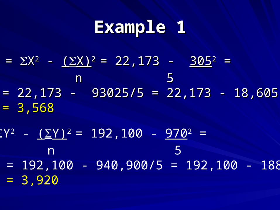
Example 1Example 1

SSSSX X = = XX22 - - ((X)X)2 2 = 22,173 - = 22,173 - 30530522 = =

nn 5 5= 22,173 - 93025/5 = 22,173 - 18,605= 22,173 - 93025/5 = 22,173 - 18,605= 3,568= 3,568

SSY = Y2 - (Y)2 = 192,100 - 9702 = n 5

= 192,100 - 940,900/5 = 192,100 - 188,180 = 3,920

Example 1Example 1

SP = SP = XY - XY - ((X)(X)(Y)Y) = =

nn

62,700 - 62,700 - (305)(970)(305)(970)

55

= 62,700 - 295,850/5 = 62,700 - 59,170= 62,700 - 295,850/5 = 62,700 - 59,170

= 3,530= 3,530

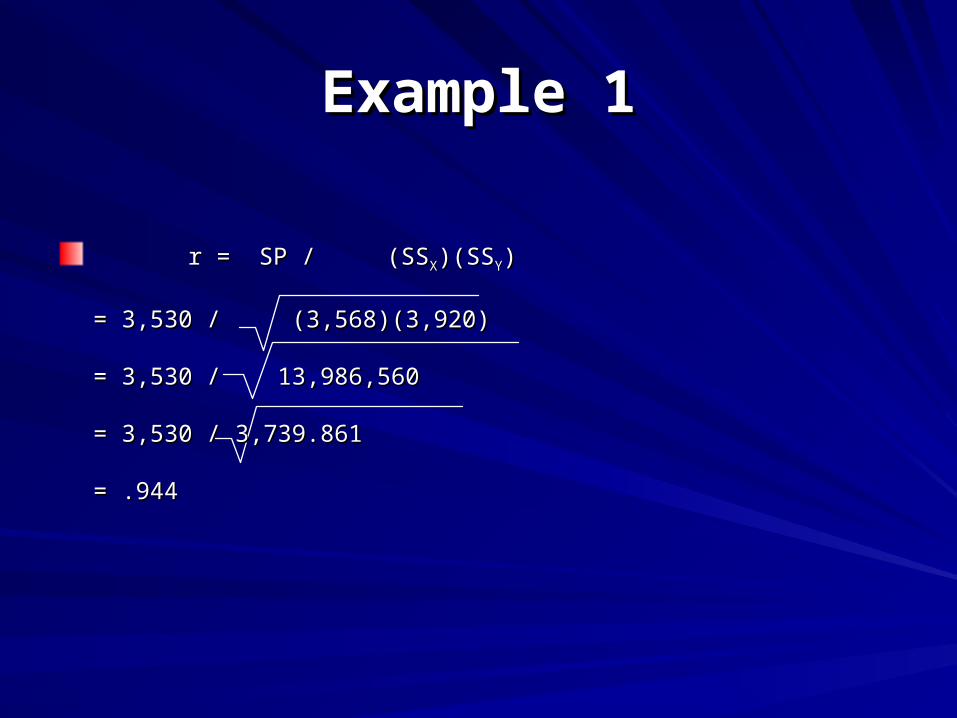
Example 1Example 1

r = SP / (SSr = SP / (SSXX)(SS)(SSYY))

= 3,530 / (3,568)(3,920)= 3,530 / (3,568)(3,920)

= 3,530 / 13,986,560= 3,530 / 13,986,560

= 3,530 / 3,739.861= 3,530 / 3,739.861

= .944= .944

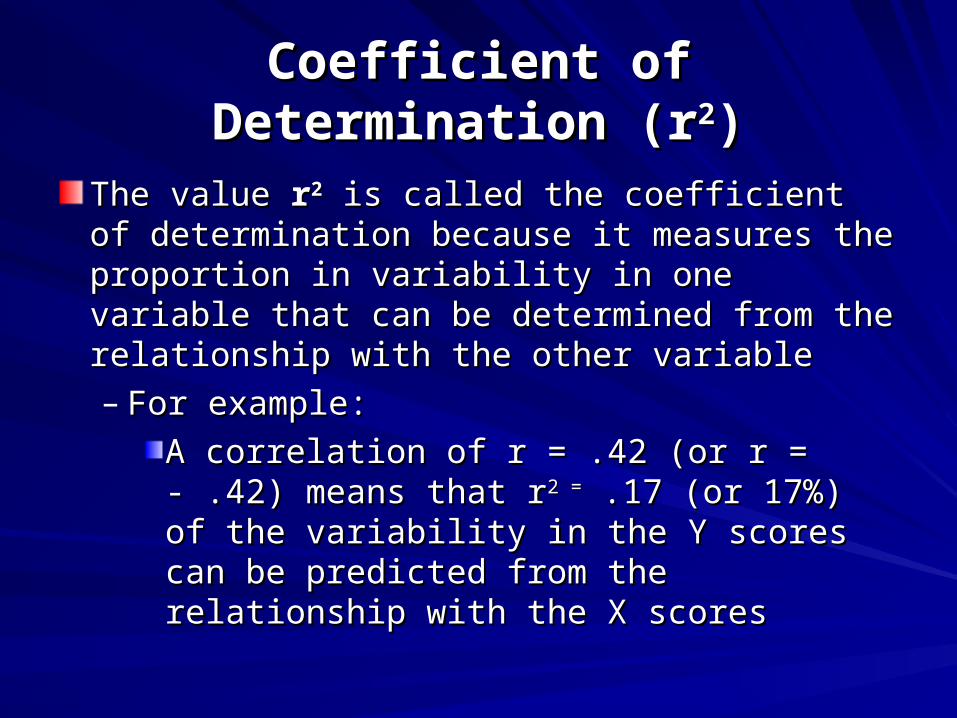
Coefficient of Determination (rCoefficient of Determination (r22))

The value The value rr22 is called the coefficient of is called the coefficient of determination because it measures the determination because it measures the proportion in variability in one variable that can proportion in variability in one variable that can be determined from the relationship with the be determined from the relationship with the other variableother variable– For example:For example:

A correlation of r = .42 (or r = - .42) means A correlation of r = .42 (or r = - .42) means that rthat r2 =2 = .17 (or 17%) of the variability in the .17 (or 17%) of the variability in the Y scores can be predicted from the Y scores can be predicted from the relationship with the X scoresrelationship with the X scores

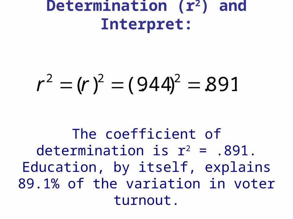
Coefficient of Determination (r2) and Interpret:

The coefficient of determination is r2 = .891. Education, by itself, explains

89.1% of the variation in voter turnout.

891.)944(.)( 222 rr

Example 2Example 2

A researcher predicts that there is a high A researcher predicts that there is a high correlation between years of education and voter correlation between years of education and voter turnoutturnout– She chooses Alamosa, Boston, Chicago, Detroit, and She chooses Alamosa, Boston, Chicago, Detroit, and

NYC to test her theoryNYC to test her theory

Example 2Example 2

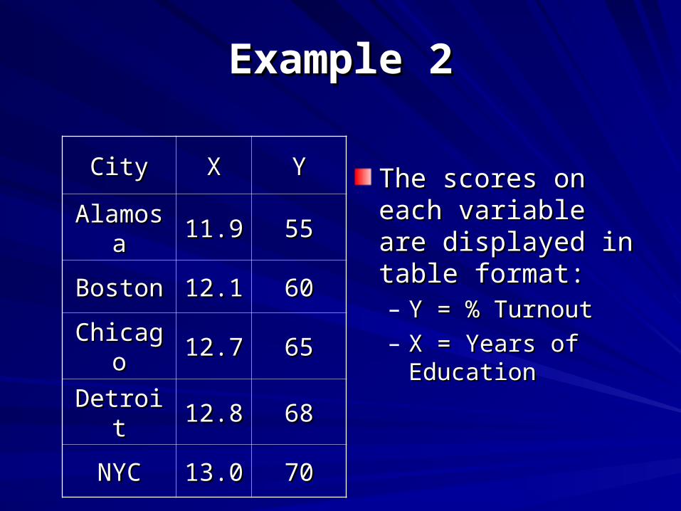
The scores on each The scores on each variable are displayed variable are displayed in table format:in table format:– Y = % TurnoutY = % Turnout– X = Years of X = Years of

EducationEducation

CityCity XX YY

AlamosaAlamosa 11.911.9 5555

BostonBoston 12.112.1 6060

ChicagoChicago 12.712.7 6565

DetroitDetroit 12.812.8 6868

NYCNYC 13.013.0 7070

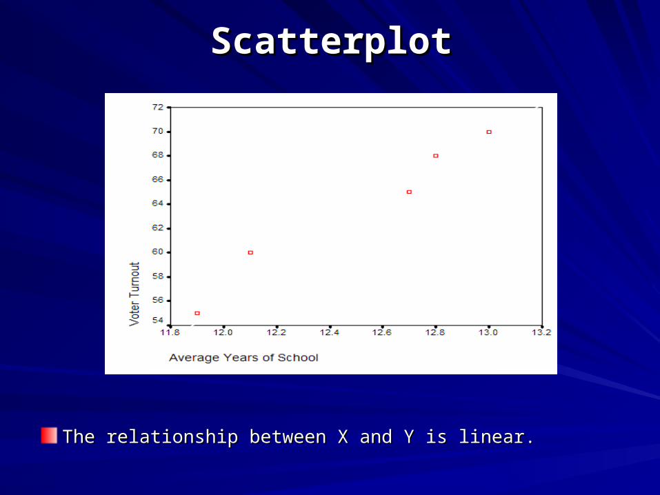
ScatterplotScatterplot

The relationship between X and Y is linear. The relationship between X and Y is linear.

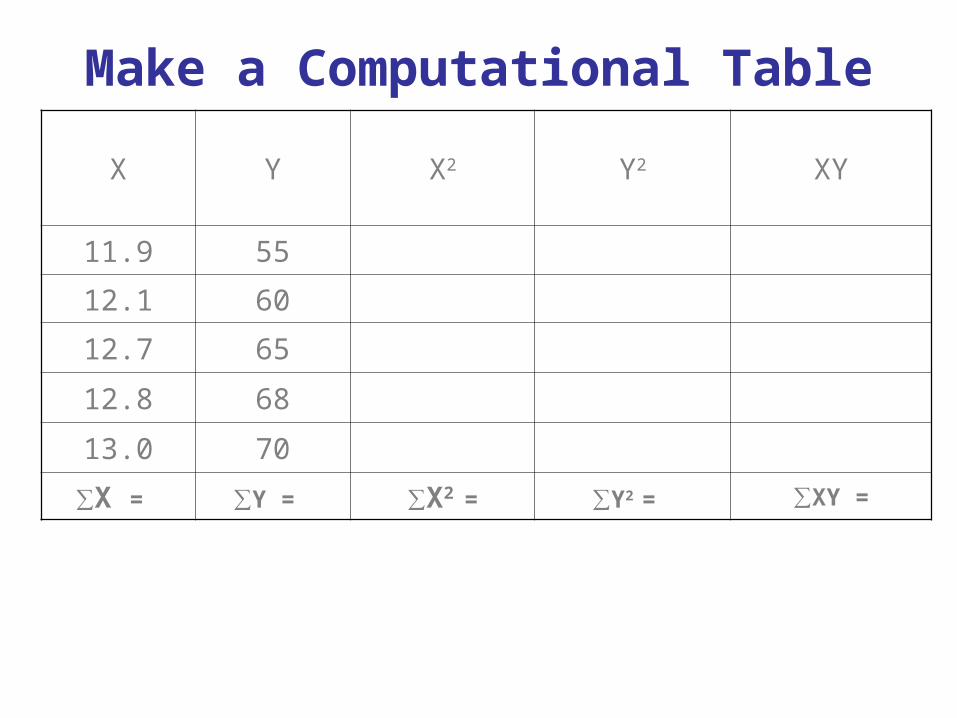
Make a Computational Table

X Y X2 Y2 XY

11.9 55

12.1 60

12.7 65

12.8 68

13.0 70

∑X = ∑Y = ∑X2 = ∑Y2 = ∑XY =

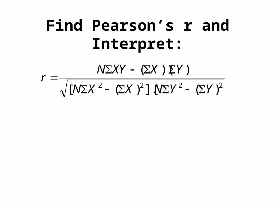
Find Pearson’s r and Interpret:

2222 )(][)([

))((

YYNXXN

YXXYNr

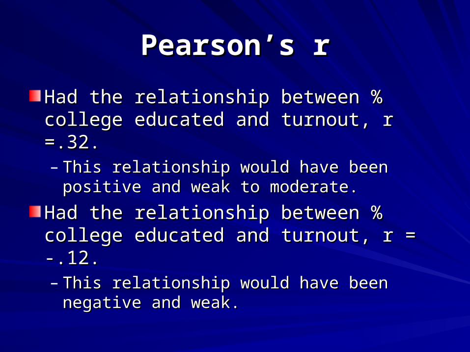
Pearson’s rPearson’s r

Had the relationship between % college Had the relationship between % college educated and turnout, r =.32.educated and turnout, r =.32.– This relationship would have been positive This relationship would have been positive

and weak to moderate.and weak to moderate.

Had the relationship between % college Had the relationship between % college educated and turnout, r = -.12.educated and turnout, r = -.12.– This relationship would have been negative This relationship would have been negative

and weak.and weak.

Find the Coefficient of Determination (r2) and Interpret:

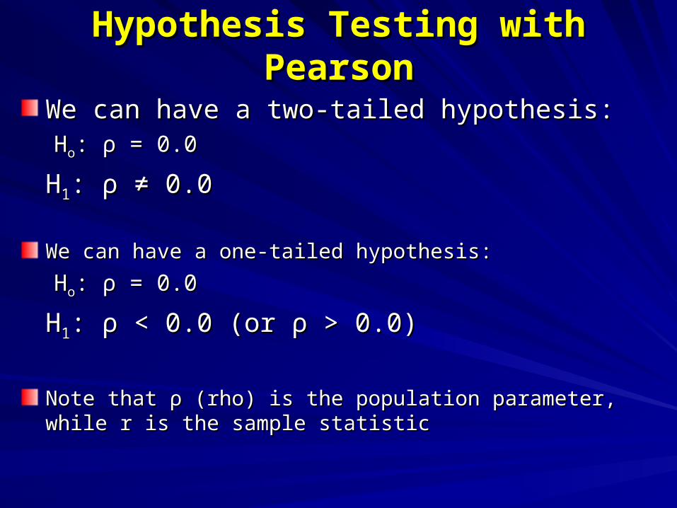
Hypothesis Testing with PearsonHypothesis Testing with Pearson

We can have a two-tailed hypothesis:We can have a two-tailed hypothesis:HHoo: : ρρ = 0.0 = 0.0

HH11: : ρρ ≠ 0.0 ≠ 0.0

We can have a one-tailed hypothesis:We can have a one-tailed hypothesis:

HHoo: : ρρ = 0.0 = 0.0

HH11: : ρρ < 0.0 (or < 0.0 (or ρρ > 0.0) > 0.0)

Note that Note that ρρ (rho) is the population parameter, while r is the (rho) is the population parameter, while r is the sample statisticsample statistic

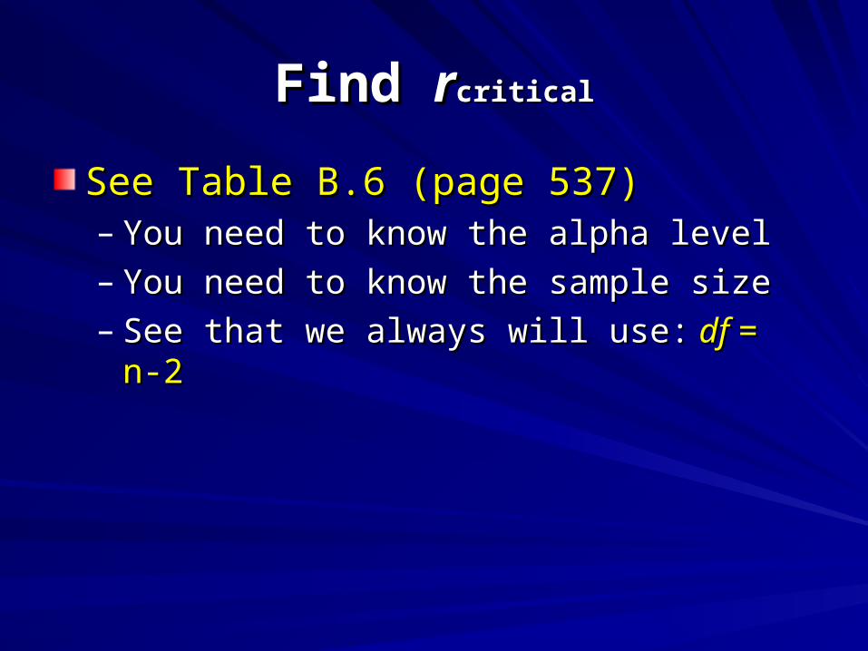
Find Find rrcriticalcritical

See Table B.6 (page 537)See Table B.6 (page 537)– You need to know the alpha levelYou need to know the alpha level– You need to know the sample sizeYou need to know the sample size– See that we always will use:See that we always will use: df df = n-2= n-2

Find Find rrcalculatedcalculated

See previous slides for formulasSee previous slides for formulas

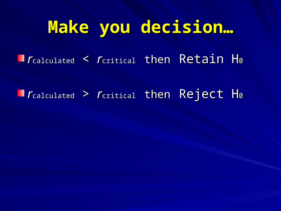
Make you decision…Make you decision…

rrcalculatedcalculated < < rrcritical critical thenthen Retain HRetain H00

rrcalculatedcalculated > > rrcritical critical thenthen Reject HReject H00

Always include a brief summary Always include a brief summary of your results:of your results:

Was it positive or negative?Was it positive or negative?

Was it significant ?Was it significant ?

Explain the correlationExplain the correlation

Explain the variationExplain the variation– Coefficient of Determination (rCoefficient of Determination (r22))

CreditsCredits

http://campus.houghton.edu/orgs/psychology/stat15b.ppt#267,2,Reviewhttp://campus.houghton.edu/orgs/psychology/stat15b.ppt#267,2,Review

http://publish.uwo.ca/~pakvis/Interval.ppt#276,17,Practical Example using http://publish.uwo.ca/~pakvis/Interval.ppt#276,17,Practical Example using Healey P. 418 Problem 15.1Healey P. 418 Problem 15.1