Embed Size (px)
Citation preview
SAS/STAT® 13.1 User’s GuideIntroduction to StatisticalModeling with SAS/STATSoftware

This document is an individual chapter from SAS/STAT® 13.1 User’s Guide.
The correct bibliographic citation for the complete manual is as follows: SAS Institute Inc. 2013. SAS/STAT® 13.1 User’s Guide.Cary, NC: SAS Institute Inc.
Copyright © 2013, SAS Institute Inc., Cary, NC, USA
All rights reserved. Produced in the United States of America.
For a hard-copy book: No part of this publication may be reproduced, stored in a retrieval system, or transmitted, in any form or byany means, electronic, mechanical, photocopying, or otherwise, without the prior written permission of the publisher, SAS InstituteInc.
For a web download or e-book: Your use of this publication shall be governed by the terms established by the vendor at the timeyou acquire this publication.
The scanning, uploading, and distribution of this book via the Internet or any other means without the permission of the publisher isillegal and punishable by law. Please purchase only authorized electronic editions and do not participate in or encourage electronicpiracy of copyrighted materials. Your support of others’ rights is appreciated.
U.S. Government License Rights; Restricted Rights: The Software and its documentation is commercial computer softwaredeveloped at private expense and is provided with RESTRICTED RIGHTS to the United States Government. Use, duplication ordisclosure of the Software by the United States Government is subject to the license terms of this Agreement pursuant to, asapplicable, FAR 12.212, DFAR 227.7202-1(a), DFAR 227.7202-3(a) and DFAR 227.7202-4 and, to the extent required under U.S.federal law, the minimum restricted rights as set out in FAR 52.227-19 (DEC 2007). If FAR 52.227-19 is applicable, this provisionserves as notice under clause (c) thereof and no other notice is required to be affixed to the Software or documentation. TheGovernment’s rights in Software and documentation shall be only those set forth in this Agreement.
SAS Institute Inc., SAS Campus Drive, Cary, North Carolina 27513-2414.
December 2013
SAS provides a complete selection of books and electronic products to help customers use SAS® software to its fullest potential. Formore information about our offerings, visit support.sas.com/bookstore or call 1-800-727-3228.
SAS® and all other SAS Institute Inc. product or service names are registered trademarks or trademarks of SAS Institute Inc. in theUSA and other countries. ® indicates USA registration.
Other brand and product names are trademarks of their respective companies.

SAS and all other SAS Institute Inc. product or service names are registered trademarks or trademarks of SAS Institute Inc. in the USA and other countries. ® indicates USA registration. Other brand and product names are trademarks of their respective companies. © 2013 SAS Institute Inc. All rights reserved. S107969US.0613
Discover all that you need on your journey to knowledge and empowerment.
support.sas.com/bookstorefor additional books and resources.
Gain Greater Insight into Your SAS® Software with SAS Books.

Chapter 3
Introduction to Statistical Modeling withSAS/STAT Software
ContentsOverview: Statistical Modeling . . . . . . . . . . . . . . . . . . . . . . . . . . . . . . . . . 24
Statistical Models . . . . . . . . . . . . . . . . . . . . . . . . . . . . . . . . . . . . 24Classes of Statistical Models . . . . . . . . . . . . . . . . . . . . . . . . . . . . . . . 27
Linear and Nonlinear Models . . . . . . . . . . . . . . . . . . . . . . . . . . 27Regression Models and Models with Classification Effects . . . . . . . . . . 28Univariate and Multivariate Models . . . . . . . . . . . . . . . . . . . . . . 30Fixed, Random, and Mixed Models . . . . . . . . . . . . . . . . . . . . . . 31Generalized Linear Models . . . . . . . . . . . . . . . . . . . . . . . . . . . 33Latent Variable Models . . . . . . . . . . . . . . . . . . . . . . . . . . . . . 33Bayesian Models . . . . . . . . . . . . . . . . . . . . . . . . . . . . . . . . 36
Classical Estimation Principles . . . . . . . . . . . . . . . . . . . . . . . . . . . . . 37Least Squares . . . . . . . . . . . . . . . . . . . . . . . . . . . . . . . . . . 37Likelihood . . . . . . . . . . . . . . . . . . . . . . . . . . . . . . . . . . . 39Inference Principles for Survey Data . . . . . . . . . . . . . . . . . . . . . . 42
Statistical Background . . . . . . . . . . . . . . . . . . . . . . . . . . . . . . . . . . . . . 43Hypothesis Testing and Power . . . . . . . . . . . . . . . . . . . . . . . . . . . . . . 43Important Linear Algebra Concepts . . . . . . . . . . . . . . . . . . . . . . . . . . . 44Expectations of Random Variables and Vectors . . . . . . . . . . . . . . . . . . . . . 51Mean Squared Error . . . . . . . . . . . . . . . . . . . . . . . . . . . . . . . . . . . 53Linear Model Theory . . . . . . . . . . . . . . . . . . . . . . . . . . . . . . . . . . 55
Finding the Least Squares Estimators . . . . . . . . . . . . . . . . . . . . . 55Analysis of Variance . . . . . . . . . . . . . . . . . . . . . . . . . . . . . . 57Estimating the Error Variance . . . . . . . . . . . . . . . . . . . . . . . . . 58Maximum Likelihood Estimation . . . . . . . . . . . . . . . . . . . . . . . 58Estimable Functions . . . . . . . . . . . . . . . . . . . . . . . . . . . . . . 59Test of Hypotheses . . . . . . . . . . . . . . . . . . . . . . . . . . . . . . . 59Residual Analysis . . . . . . . . . . . . . . . . . . . . . . . . . . . . . . . . 62Sweep Operator . . . . . . . . . . . . . . . . . . . . . . . . . . . . . . . . . 64
References . . . . . . . . . . . . . . . . . . . . . . . . . . . . . . . . . . . . . . . . . . . 65
24 F Chapter 3: Introduction to Statistical Modeling with SAS/STAT Software
Overview: Statistical ModelingThere are more than 70 procedures in SAS/STAT software, and the majority of them are dedicated to solvingproblems in statistical modeling. The goal of this chapter is to provide a roadmap to statistical models and tomodeling tasks, enabling you to make informed choices about the appropriate modeling context and tool. Thischapter also introduces important terminology, notation, and concepts used throughout this documentation.Subsequent introductory chapters discuss model families and related procedures.
It is difficult to capture the complexity of statistical models in a simple scheme, so the classification usedhere is necessarily incomplete. It is most practical to classify models in terms of simple criteria, such as thepresence of random effects, the presence of nonlinearity, characteristics of the data, and so on. That is theapproach used here. After a brief introduction to statistical modeling in general terms, the chapter describes anumber of model classifications and relates them to modeling tools in SAS/STAT software.
Statistical Models
Deterministic and Stochastic Models
Purely mathematical models, in which the relationships between inputs and outputs are captured entirelyin deterministic fashion, can be important theoretical tools but are impractical for describing observational,experimental, or survey data. For such phenomena, researchers usually allow the model to draw on stochasticas well as deterministic elements. When the uncertainty of realizations leads to the inclusion of randomcomponents, the resulting models are called stochastic models. A statistical model, finally, is a stochasticmodel that contains parameters, which are unknown constants that need to be estimated based on assumptionsabout the model and the observed data.
There are many reasons why statistical models are preferred over deterministic models. For example:
• Randomness is often introduced into a system in order to achieve a certain balance or representativeness.For example, random assignment of treatments to experimental units allows unbiased inferences abouttreatment effects. As another example, selecting individuals for a survey sample by random mechanismsensures a representative sample.
• Even if a deterministic model can be formulated for the phenomenon under study, a stochastic modelcan provide a more parsimonious and more easily comprehended description. For example, it ispossible in principle to capture the result of a coin toss with a deterministic model, taking into accountthe properties of the coin, the method of tossing, conditions of the medium through which the cointravels and of the surface on which it lands, and so on. A very complex model is required to describethe simple outcome—heads or tails. Alternatively, you can describe the outcome quite simply as theresult of a stochastic process, a Bernoulli variable that results in heads with a certain probability.
• It is often sufficient to describe the average behavior of a process, rather than each particular realization.For example, a regression model might be developed to relate plant growth to nutrient availability.The explicit aim of the model might be to describe how the average growth changes with nutrientavailability, not to predict the growth of an individual plant. The support for the notion of averaging ina model lies in the nature of expected values, describing typical behavior in the presence of randomness.This, in turn, requires that the model contain stochastic components.
Statistical Models F 25
The defining characteristic of statistical models is their dependence on parameters and the incorporation ofstochastic terms. The properties of the model and the properties of quantities derived from it must be studiedin a long-run, average sense through expectations, variances, and covariances. The fact that the parameters ofthe model must be estimated from the data introduces a stochastic element in applying a statistical model:because the model is not deterministic but includes randomness, parameters and related quantities derivedfrom the model are likewise random. The properties of parameter estimators can often be described onlyin an asymptotic sense, imagining that some aspect of the data increases without bound (for example, thenumber of observations or the number of groups).
The process of estimating the parameters in a statistical model based on your data is called fitting the model.For many classes of statistical models there are a number of procedures in SAS/STAT software that canperform the fitting. In many cases, different procedures solve identical estimation problems—that is, theirparameter estimates are identical. In some cases, the same model parameters are estimated by differentstatistical principles, such as least squares versus maximum likelihood estimation. Parameter estimatesobtained by different methods typically have different statistical properties—distribution, variance, bias, andso on. The choice between competing estimation principles is often made on the basis of properties of theestimators. Distinguishing properties might include (but are not necessarily limited to) computational ease,interpretive ease, bias, variance, mean squared error, and consistency.
Model-Based and Design-Based Randomness
A statistical model is a description of the data-generating mechanism, not a description of the specific data towhich it is applied. The aim of a model is to capture those aspects of a phenomenon that are relevant to inquiryand to explain how the data could have come about as a realization of a random experiment. These relevantaspects might include the genesis of the randomness and the stochastic effects in the phenomenon understudy. Different schools of thought can lead to different model formulations, different analytic strategies,and different results. Coarsely, you can distinguish between a viewpoint of innate randomness and one ofinduced randomness. This distinction leads to model-based and design-based inference approaches.
In a design-based inference framework, the random variation in the observed data is induced by randomselection or random assignment. Consider the case of a survey sample from a finite population of sizeN; suppose that FN D fyi W i 2 UN g denotes the finite set of possible values and UN is the index setUN D f1; 2; : : : ; N g. Then a sample S, a subset of UN , is selected by probability rules. The realizationof the random experiment is the selection of a particular set S; the associated values selected from FN areconsidered fixed. If properties of a design-based sampling estimator are evaluated, such as bias, variance, andmean squared error, they are evaluated with respect to the distribution induced by the sampling mechanism.
Design-based approaches also play an important role in the analysis of data from controlled experiments byrandomization tests. Suppose that k treatments are to be assigned to kr homogeneous experimental units. Ifyou form k sets of r units with equal probability, and you assign the jth treatment to the tth set, a completelyrandomized experimental design (CRD) results. A design-based view treats the potential response of aparticular treatment for a particular experimental unit as a constant. The stochastic nature of the error-controldesign is induced by randomly selecting one of the potential responses.
Statistical models are often used in the design-based framework. In a survey sample the model is used tomotivate the choice of the finite population parameters and their sample-based estimators. In an experimentaldesign, an assumption of additivity of the contributions from treatments, experimental units, observationalerrors, and experimental errors leads to a linear statistical model. The approach to statistical inferencewhere statistical models are used to construct estimators and their properties are evaluated with respect to
26 F Chapter 3: Introduction to Statistical Modeling with SAS/STAT Software
the distribution induced by the sample selection mechanism is known as model-assisted inference (Särndal,Swensson, and Wretman 1992).
In a purely model-based framework, the only source of random variation for inference comes from the un-known variation in the responses. Finite population values are thought of as a realization of a superpopulationmodel that describes random variables Y1; Y2; � � � . The observed values y1; y2; � � � are realizations of theserandom variables. A model-based framework does not imply that there is only one source of random variationin the data. For example, mixed models might contain random terms that represent selection of effects fromhierarchical (super-) populations at different granularity. The analysis takes into account the hierarchicalstructure of the random variation, but it continues to be model based.
A design-based approach is implicit in SAS/STAT procedures whose name commences with SURVEY, suchas the SURVEYFREQ, SURVEYMEANS, SURVEYREG, SURVEYLOGISTIC, and SURVEYPHREGprocedures. Inferential approaches are model based in other SAS/STAT procedures. For more informationabout analyzing survey data with SAS/STAT software, see Chapter 14, “Introduction to Survey Procedures.”
Model Specification
If the model is accepted as a description of the data-generating mechanism, then its parameters are estimatedusing the data at hand. Once the parameter estimates are available, you can apply the model to answerquestions of interest about the study population. In other words, the model becomes the lens through whichyou view the problem itself, in order to ask and answer questions of interest. For example, you might use theestimated model to derive new predictions or forecasts, to test hypotheses, to derive confidence intervals, andso on.
Obviously, the model must be “correct” to the extent that it sufficiently describes the data-generatingmechanism. Model selection, diagnosis, and discrimination are important steps in the model-building process.This is typically an iterative process, starting with an initial model and refining it. The first important stepis thus to formulate your knowledge about the data-generating process and to express the real observedphenomenon in terms of a statistical model. A statistical model describes the distributional properties of oneor more variables, the response variables. The extent of the required distributional specification depends onthe model, estimation technique, and inferential goals. This description often takes the simple form of amodel with additive error structure:
response = mean + error
In mathematical notation this simple model equation becomes
Y D f .x1; � � � ; xkIˇ1; � � � ; ˇp/C �
In this equation Y is the response variable, often also called the dependent variable or the outcome variable.The terms x1; � � � ; xk denote the values of k regressor variables, often termed the covariates or the “indepen-dent” variables. The terms ˇ1; � � � ; ˇp denote parameters of the model, unknown constants that are to beestimated. The term � denotes the random disturbance of the model; it is also called the residual term or theerror term of the model.
In this simple model formulation, stochastic properties are usually associated only with the � term. Thecovariates x1; � � � ; xk are usually known values, not subject to random variation. Even if the covariates aremeasured with error, so that their values are in principle random, they are considered fixed in most models fitby SAS/STAT software. In other words, stochastic properties under the model are derived conditional on the
Classes of Statistical Models F 27
xs. If � is the only stochastic term in the model, and if the errors have a mean of zero, then the function f .�/is the mean function of the statistical model. More formally,
EŒY � D f .x1; � � � ; xkIˇ1; � � � ; ˇp/
where EŒ�� denotes the expectation operator.
In many applications, a simple model formulation is inadequate. It might be necessary to specify not only thestochastic properties of a single error term, but also how model errors associated with different observationsrelate to each other. A simple additive error model is typically inappropriate to describe the data-generatingmechanism if the errors do not have zero mean or if the variance of observations depends on their means.For example, if Y is a Bernoulli random variable that takes on the values 0 and 1 only, a regression modelwith additive error is not meaningful. Models for such data require more elaborate formulations involvingprobability distributions.
Classes of Statistical Models
Linear and Nonlinear Models
A statistical estimation problem is nonlinear if the estimating equations—the equations whose solutionyields the parameter estimates—depend on the parameters in a nonlinear fashion. Such estimation problemstypically have no closed-form solution and must be solved by iterative, numerical techniques.
Nonlinearity in the mean function is often used to distinguish between linear and nonlinear models. A modelhas a nonlinear mean function if the derivative of the mean function with respect to the parameters dependson at least one other parameter. Consider, for example, the following models that relate a response variable Yto a single regressor variable x:
EŒY jx� D ˇ0 C ˇ1x
EŒY jx� D ˇ0 C ˇ1x C ˇ2x2
EŒY jx� D ˇ C x=˛
In these expressions, EŒY jx� denotes the expected value of the response variable Y at the fixed value ofx. (The conditioning on x simply indicates that the predictor variables are assumed to be non-random.Conditioning is often omitted for brevity in this and subsequent chapters.)
The first model in the previous list is a simple linear regression (SLR) model. It is linear in the parameters ˇ0and ˇ1 since the model derivatives do not depend on unknowns:
@
ˇ0.ˇ0 C ˇ1x/ D 1
@
ˇ1.ˇ0 C ˇ1x/ D x
28 F Chapter 3: Introduction to Statistical Modeling with SAS/STAT Software
The model is also linear in its relationship with x (a straight line). The second model is also linear in theparameters, since
@
ˇ0
�ˇ0 C ˇ1x C ˇ2x
2�D 1
@
ˇ1
�ˇ0 C ˇ1x C ˇ2x
2�D x
@
ˇ2
�ˇ0 C ˇ1x C ˇ2x
2�D x2
However, this second model is curvilinear, since it exhibits a curved relationship when plotted against x. Thethird model, finally, is a nonlinear model since
@
ˇ.ˇ C x=˛/ D 1
@
˛.ˇ C x=˛/ D �
x
˛2
The second of these derivatives depends on a parameter ˛. A model is nonlinear if it is not linear in at leastone parameter. Only the third model is a nonlinear model. A graph of EŒY � versus the regressor variable thusdoes not indicate whether a model is nonlinear. A curvilinear relationship in this graph can be achieved by amodel that is linear in the parameters.
Nonlinear mean functions lead to nonlinear estimation. It is important to note, however, that nonlinearestimation arises also because of the estimation principle or because the model structure contains nonlinearityin other parts, such as the covariance structure. For example, fitting a simple linear regression model byminimizing the sum of the absolute residuals leads to a nonlinear estimation problem despite the fact that themean function is linear.
Regression Models and Models with Classification Effects
A linear regression model in the broad sense has the form
Y D Xˇ C �
where Y is the vector of response values, X is the matrix of regressor effects, ˇ is the vector of regressionparameters, and � is the vector of errors or residuals. A regression model in the narrow sense—as comparedto a classification model—is a linear model in which all regressor effects are continuous variables. In otherwords, each effect in the model contributes a single column to the X matrix and a single parameter to theoverall model. For example, a regression of subjects’ weight (Y) on the regressors age (x1) and body massindex (bmi, x2) is a regression model in this narrow sense. In symbolic notation you can write this regressionmodel as
weight = age + bmi + error
This symbolic notation expands into the statistical model
Yi D ˇ0 C ˇ1xi1 C ˇ2xi2 C �i
Classes of Statistical Models F 29
Single parameters are used to model the effects of age .ˇ1/ and bmi .ˇ2/, respectively.
A classification effect, on the other hand, is associated with possibly more than one column of the X matrix.Classification with respect to a variable is the process by which each observation is associated with one of klevels; the process of determining these k levels is referred to as levelization of the variable. Classificationvariables are used in models to identify experimental conditions, group membership, treatments, and soon. The actual values of the classification variable are not important, and the variable can be a numeric ora character variable. What is important is the association of discrete values or levels of the classificationvariable with groups of observations. For example, in the previous illustration, if the regression also takes intoaccount the subjects’ gender, this can be incorporated in the model with a two-level classification variable.Suppose that the values of the gender variable are coded as ‘F’ and ‘M’, respectively. In symbolic notationthe model
weight = age + bmi + gender + error
expands into the statistical model
Yi D ˇ0 C ˇ1xi1 C ˇ2xi2 C �1I.gender D 0F0/C �2I.gender D 0M0/C �i
where I(gender=‘F’) is the indicator function that returns 1 if the value of the gender variable is ‘F’ and0 otherwise. Parameters �1 and �2 are associated with the gender classification effect. This form ofparameterizing the gender effect in the model is only one of several different methods of incorporatingthe levels of a classification variable in the model. This form, the so-called singular parameterization, isthe most general approach, and it is used in the GLM, MIXED, and GLIMMIX procedures. Alternatively,classification effects with various forms of nonsingular parameterizations are available in such proceduresas GENMOD and LOGISTIC. See the documentation for the individual SAS/STAT procedures on theirrespective facilities for parameterizing classification variables and the section “Parameterization of ModelEffects” on page 387 in Chapter 19, “Shared Concepts and Topics,” for general details.
Models that contain only classification effects are often identified with analysis of variance (ANOVA) models,because ANOVA methods are frequently used in their analysis. This is particularly true for experimental datawhere the model effects comprise effects of the treatment and error-control design. However, classificationeffects appear more widely than in models to which analysis of variance methods are applied. For example,many mixed models, where parameters are estimated by restricted maximum likelihood, consist entirely ofclassification effects but do not permit the sum of squares decomposition typical for ANOVA techniques.
Many models contain both continuous and classification effects. For example, a continuous-by-classeffect consists of at least one continuous variable and at least one classification variable. Such effects areconvenient, for example, to vary slopes in a regression model by the levels of a classification variable. Also,recent enhancements to linear modeling syntax in some SAS/STAT procedures (including GLIMMIX andGLMSELECT) enable you to construct sets of columns in X matrices from a single continuous variable. Anexample is modeling with splines where the values of a continuous variable x are expanded into a spline basisthat occupies multiple columns in the X matrix. For purposes of the analysis you can treat these columns as asingle unit or as individual, unrelated columns. For more details, see the section “EFFECT Statement” onpage 397 in Chapter 19, “Shared Concepts and Topics.”
30 F Chapter 3: Introduction to Statistical Modeling with SAS/STAT Software
Univariate and Multivariate Models
A multivariate statistical model is a model in which multiple response variables are modeled jointly. Suppose,for example, that your data consist of heights .hi / and weights .wi / of children, collected over several years.ti /. The following separate regressions represent two univariate models:
wi D ˇw0 C ˇw1ti C �wi
hi D ˇh0 C ˇh1ti C �hi
In the univariate setting, no information about the children’s heights “flows” to the model about their weightsand vice versa. In a multivariate setting, the heights and weights would be modeled jointly. For example:
Yi D�wihi
�D Xˇ C
��wi�hi
�D Xˇ C �i
�i �
�0;��21 �12�12 �22
��The vectors Yi and �i collect the responses and errors for the two observation that belong to the same subject.The errors from the same child now have the correlation
CorrŒ�wi ; �hi � D�12q�21 �
22
and it is through this correlation that information about heights “flows” to the weights and vice versa. Thissimple example shows only one approach to modeling multivariate data, through the use of covariancestructures. Other techniques involve seemingly unrelated regressions, systems of linear equations, and so on.
Multivariate data can be coarsely classified into three types. The response vectors of homogeneous mul-tivariate data consist of observations of the same attribute. Such data are common in repeated measuresexperiments and longitudinal studies, where the same attribute is measured repeatedly over time. Homo-geneous multivariate data also arise in spatial statistics where a set of geostatistical data is the incompleteobservation of a single realization of a random experiment that generates a two-dimensional surface. Onehundred measurements of soil electrical conductivity collected in a forest stand compose a single observationof a 100-dimensional homogeneous multivariate vector. Heterogeneous multivariate observations arisewhen the responses that are modeled jointly refer to different attributes, such as in the previous example ofchildren’s weights and heights. There are two important subtypes of heterogeneous multivariate data. Inhomocatanomic multivariate data the observations come from the same distributional family. For example,the weights and heights might both be assumed to be normally distributed. With heterocatanomic multivari-ate data the observations can come from different distributional families. The following are examples ofheterocatanomic multivariate data:
• For each patient you observe blood pressure (a continuous outcome), the number of prior episodes ofan illness (a count variable), and whether the patient has a history of diabetes in the family (a binaryoutcome). A multivariate model that models the three attributes jointly might assume a lognormaldistribution for the blood pressure measurements, a Poisson distribution for the count variable and aBernoulli distribution for the family history.
• In a study of HIV/AIDS survival, you model jointly a patient’s CD4 cell count over time—itself ahomogeneous multivariate outcome—and the survival of the patient (event-time data).
Classes of Statistical Models F 31
Fixed, Random, and Mixed Models
Each term in a statistical model represents either a fixed effect or a random effect. Models in which all effectsare fixed are called fixed-effects models. Similarly, models in which all effects are random—apart frompossibly an overall intercept term—are called random-effects models. Mixed models, then, are those modelsthat have fixed-effects and random-effects terms. In matrix notation, the linear fixed, linear random, andlinear mixed model are represented by the following model equations, respectively:
Y D Xˇ C �
Y D Z C �Y D Xˇ C Z C �
In these expressions, X and Z are design or regressor matrices associated with the fixed and random effects,respectively. The vector ˇ is a vector of fixed-effects parameters, and the vector represents the randomeffects. The mixed modeling procedures in SAS/STAT software assume that the random effects follow anormal distribution with variance-covariance matrix G and, in most cases, that the random effects have meanzero.
Random effects are often associated with classification effects, but this is not necessary. As an exampleof random regression effects, you might want to model the slopes in a growth model as consisting of twocomponents: an overall (fixed-effects) slope that represents the slope of the average individual, and individual-specific random deviations from the overall slope. The X and Z matrix would then have column entries forthe regressor variable associated with the slope. You are modeling fixed and randomly varying regressioncoefficients.
Having random effects in your model has a number of important consequences:
• Some observations are no longer uncorrelated but instead have a covariance that depends on thevariance of the random effects.
• You can and should distinguish between the inference spaces; inferences can be drawn in a broad,intermediate, and narrow inference space. In the narrow inference space, conclusions are drawn aboutthe particular values of the random effects selected in the study. The broad inference space appliesif inferences are drawn with respect to all possible levels of the random effects. The intermediateinference space can be applied for effects consisting of more than one random term, when inferencesare broad with respect to some factors and narrow with respect to others. In fixed-effects models, thereis no corresponding concept to the broad and intermediate inference spaces.
• Depending on the structure of G and VarŒ�� and also subject to the balance in your data, there mightbe no closed-form solution for the parameter estimates. Although the model is linear in ˇ, iterativeestimation methods might be required to estimate all parameters of the model.
• Certain concepts, such as least squares means and Type III estimable functions, are meaningful onlyfor fixed effects.
• By using random effects, you are modeling variation through variance. Variation in data simply impliesthat things are not equal. Variance, on the other hand, describes a feature of a random variable. Randomeffects in your model are random variables: they model variation through variance.
It is important to properly determine the nature of the model effects as fixed or random. An effect is eitherfixed or random by its very nature; it is improper to consider it fixed in one analysis and random in another
32 F Chapter 3: Introduction to Statistical Modeling with SAS/STAT Software
depending on what type of results you want to produce. If, for example, a treatment effect is random andyou are interested in comparing treatment means, and only the levels selected in the study are of interest,then it is not appropriate to model the treatment effect as fixed so that you can draw on least squares meananalysis. The appropriate strategy is to model the treatment effect as random and to compare the solutions forthe treatment effects in the narrow inference space.
In determining whether an effect is fixed or random, it is helpful to inquire about the genesis of the effect. Ifthe levels of an effect are randomly sampled, then the effect is a random effect. The following are examples:
• In a large clinical trial, drugs A, B, and C are applied to patients in various clinical centers. If theclinical centers are selected at random from a population of possible clinics, their effect on the responseis modeled with a random effect.
• In repeated measures experiments with people or animals as subjects, subjects are declared to berandom because they are selected from the larger population to which you want to generalize.
• Fertilizers could be applied at a number of levels. Three levels are randomly selected for an experimentto represent the population of possible levels. The fertilizer effects are random effects.
Quite often it is not possible to select effects at random, or it is not known how the values in the data becamepart of the study. For example, suppose you are presented with a data set consisting of student scores in threeschool districts, with four to ten schools in each district and two to three classrooms in each school. How doyou decide which effects are fixed and which are random? As another example, in an agricultural experimentconducted in successive years at two locations, how do you decide whether location and year effects arefixed or random? In these situations, the fixed or random nature of the effect might be debatable, bearing outthe adage that “one modeler’s fixed effect is another modeler’s random effect.” However, this fact does notconstitute license to treat as random those effects that are clearly fixed, or vice versa.
When an effect cannot be randomized or it is not known whether its levels have been randomly selected, itcan be a random effect if its impact on the outcome variable is of a stochastic nature—that is, if it is therealization of a random process. Again, this line of thinking relates to the genesis of the effect. A randomyear, location, or school district effect is a placeholder for different environments that cannot be selectedat random but whose effects are the cumulative result of many individual random processes. Note that thisargument does not imply that effects are random because the experimenter does not know much about them.The key notion is that effects represent something, whether or not that something is known to the modeler.Broadening the inference space beyond the observed levels is thus possible, although you might not be ableto articulate what the realizations of the random effects represent.
A consequence of having random effects in your model is that some observations are no longer uncorrelatedbut instead have a covariance that depends on the variance of the random effect. In fact, in some modelingapplications random effects might be used not only to model heterogeneity in the parameters of a model, butalso to induce correlations among observations. The typical assumption about random effects in SAS/STATsoftware is that the effects are normally distributed.
For more information about mixed modeling tools in SAS/STAT software, see Chapter 6, “Introduction toMixed Modeling Procedures.”
Classes of Statistical Models F 33
Generalized Linear Models
A class of models that has gained increasing importance in the past several decades is the class of generalizedlinear models. The theory of generalized linear models originated with Nelder and Wedderburn (1972);Wedderburn (1974), and was subsequently made popular in the monograph by McCullagh and Nelder (1989).This class of models extends the theory and methods of linear models to data with nonnormal responses.Before this theory was developed, modeling of nonnormal data typically relied on transformations of the data,and the transformations were chosen to improve symmetry, homogeneity of variance, or normality. Suchtransformations have to be performed with care because they also have implications for the error structure ofthe model, Also, back-transforming estimates or predicted values can introduce bias.
Generalized linear models also apply a transformation, known as the link function, but it is applied to adeterministic component, the mean of the data. Furthermore, generalized linear models take the distributionof the data into account, rather than assuming that a transformation of the data leads to normally distributeddata to which standard linear modeling techniques can be applied.
To put this generalization in place requires a slightly more sophisticated model setup than that required forlinear models for normal data:
• The systematic component is a linear predictor similar to that in linear models, � D x0ˇ. The linearpredictor is a linear function in the parameters. In contrast to the linear model, � does not represent themean function of the data.
• The link function g. � / relates the linear predictor to the mean, g.�/ D �. The link function is amonotonic, invertible function. The mean can thus be expressed as the inversely linked linear predictor,� D g�1.�/. For example, a common link function for binary and binomial data is the logit link,g.t/ D logft=.1 � t /g. The mean function of a generalized linear model with logit link and a singleregressor can thus be written as
log�
�
1 � �
�D ˇ0 C ˇ1x
� D1
1C expf�ˇ0 � ˇ1xg
This is known as a logistic regression model.
• The random component of a generalized linear model is the distribution of the data, assumed to bea member of the exponential family of distributions. Discrete members of this family include theBernoulli (binary), binomial, Poisson, geometric, and negative binomial (for a given value of the scaleparameter) distribution. Continuous members include the normal (Gaussian), beta, gamma, inverseGaussian, and exponential distribution.
The standard linear model with normally distributed error is a special case of a generalized linear model; thelink function is the identity function and the distribution is normal.
Latent Variable Models
Latent variable modeling involves variables that are not observed directly in your research. It has a relativelylong history, dating back from the measure of general intelligence by common factor analysis (Spearman1904) to the emergence of modern-day structural equation modeling (Jöreskog 1973; Keesling 1972; Wiley1973).
34 F Chapter 3: Introduction to Statistical Modeling with SAS/STAT Software
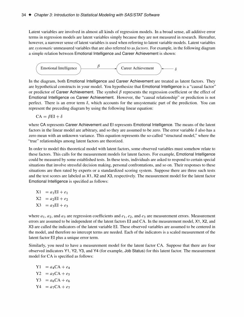
Latent variables are involved in almost all kinds of regression models. In a broad sense, all additive errorterms in regression models are latent variables simply because they are not measured in research. Hereafter,however, a narrower sense of latent variables is used when referring to latent variable models. Latent variablesare systematic unmeasured variables that are also referred to as factors. For example, in the following diagrama simple relation between Emotional Intelligence and Career Achievement is shown:
Emotional Intelligence Career Achievementˇı
In the diagram, both Emotional Intelligence and Career Achievement are treated as latent factors. Theyare hypothetical constructs in your model. You hypothesize that Emotional Intelligence is a “causal factor”or predictor of Career Achievement. The symbol ˇ represents the regression coefficient or the effect ofEmotional Intelligence on Career Achievement. However, the “causal relationship” or prediction is notperfect. There is an error term ı, which accounts for the unsystematic part of the prediction. You canrepresent the preceding diagram by using the following linear equation:
CA D ˇEIC ı
where CA represents Career Achievement and EI represents Emotional Intelligence. The means of the latentfactors in the linear model are arbitrary, and so they are assumed to be zero. The error variable ı also has azero mean with an unknown variance. This equation represents the so-called “structural model,” where the“true” relationships among latent factors are theorized.
In order to model this theoretical model with latent factors, some observed variables must somehow relate tothese factors. This calls for the measurement models for latent factors. For example, Emotional Intelligencecould be measured by some established tests. In these tests, individuals are asked to respond to certain specialsituations that involve stressful decision making, personal confrontations, and so on. Their responses to thesesituations are then rated by experts or a standardized scoring system. Suppose there are three such testsand the test scores are labeled as X1, X2 and X3, respectively. The measurement model for the latent factorEmotional Intelligence is specified as follows:
X1 D a1EIC e1X2 D a2EIC e2X3 D a3EIC e3
where a1, a2, and a3 are regression coefficients and e1, e2, and e3 are measurement errors. Measurementerrors are assumed to be independent of the latent factors EI and CA. In the measurement model, X1, X2, andX3 are called the indicators of the latent variable EI. These observed variables are assumed to be centered inthe model, and therefore no intercept terms are needed. Each of the indicators is a scaled measurement of thelatent factor EI plus a unique error term.
Similarly, you need to have a measurement model for the latent factor CA. Suppose that there are fourobserved indicators Y1, Y2, Y3, and Y4 (for example, Job Status) for this latent factor. The measurementmodel for CA is specified as follows:
Y1 D a4CAC e4Y2 D a5CAC e5Y3 D a6CAC e6Y4 D a7CAC e7
Classes of Statistical Models F 35
where a4, a5, a6, and a7 are regression coefficients and e4, e5, e6, and e7 are error terms. Again, the errorterms are assumed to be independent of the latent variables EI and CA, and Y1, Y2, Y3, and Y4 are centeredin the equations.
Given the data for the measured variables, you analyze the structural and measurement models simultaneouslyby the structural equation modeling techniques. In other words, estimation of ˇ, a1–a7, and other parametersin the model are carried out simultaneously in the modeling.
Modeling involving the use of latent factors is quite common in social and behavioral sciences, personalityassessment, and marketing research. Hypothetical constructs, although not observable, are very important inbuilding theories in these areas.
Another use of latent factors in modeling is to “purify” the predictors in regression analysis. A commonassumption in linear regression models is that predictors are measured without errors. That is, in the followinglinear equation x is assumed to have been measured without errors:
y D ˛ C ˇx C �
However, if x has been contaminated with measurement errors that cannot be ignored, the estimate of ˇmight be biased severely so that the true relationship between x and y would be masked.
A measurement model for x provides a solution to such a problem. Let Fx be a “purified” version of x. Thatis, Fx is the “true” measure of x without measurement errors, as described in the following equation:
x D Fx C ı
where ı represents a random measurement error term. Now, the linear relationship of interest is specified inthe following new linear regression equation:
y D ˛ C ˇFx C �
In this equation, Fx , which is now free from measurement errors, replaces x in the original equation. Withmeasurement errors taken into account in the simultaneous fitting of the measurement and the new regressionequations, estimation of ˇ is unbiased; hence it reflects the true relationship much better.
Certainly, introducing latent factors in models is not a “free lunch.” You must pay attention to the identificationissues induced by the latent variable methodology. That is, in order to estimate the parameters in structuralequation models with latent variables, you must set some identification constraints in these models. Thereare some established rules or conventions that would lead to proper model identification and estimation. SeeChapter 17, “Introduction to Structural Equation Modeling with Latent Variables,” for examples and generaldetails.
In addition, because of the nature of latent variables, estimation in structural equation modeling with latentvariables does not follow the same form as that of linear regression analysis. Instead of defining the estimatorsin terms of the data matrices, most estimation methods in structural equation modeling use the fitting of thefirst- and second- order moments. Hence, estimation principles described in the section “Classical EstimationPrinciples” on page 37 do not apply to structural equation modeling. However, you can see the section“Estimation Criteria” on page 1459 in Chapter 29, “The CALIS Procedure,” for details about estimation instructural equation modeling with latent variables.
36 F Chapter 3: Introduction to Statistical Modeling with SAS/STAT Software
Bayesian Models
Statistical models based on the classical (or frequentist) paradigm treat the parameters of the model as fixed,unknown constants. They are not random variables, and the notion of probability is derived in an objectivesense as a limiting relative frequency. The Bayesian paradigm takes a different approach. Model parametersare random variables, and the probability of an event is defined in a subjective sense as the degree to whichyou believe that the event is true. This fundamental difference in philosophy leads to profound differencesin the statistical content of estimation and inference. In the frequentist framework, you use the data to bestestimate the unknown value of a parameter; you are trying to pinpoint a value in the parameter space as wellas possible. In the Bayesian framework, you use the data to update your beliefs about the behavior of theparameter to assess its distributional properties as well as possible.
Suppose you are interested in estimating � from data Y D ŒY1; � � � ; Yn� by using a statistical model describedby a density p.yj�/. Bayesian philosophy states that � cannot be determined exactly, and uncertainty aboutthe parameter is expressed through probability statements and distributions. You can say, for example, that �follows a normal distribution with mean 0 and variance 1, if you believe that this distribution best describesthe uncertainty associated with the parameter.
The following steps describe the essential elements of Bayesian inference:
1. A probability distribution for � is formulated as �.�/, which is known as the prior distribution, orjust the prior. The prior distribution expresses your beliefs, for example, on the mean, the spread, theskewness, and so forth, about the parameter prior to examining the data.
2. Given the observed data Y, you choose a statistical model p.yj�/ to describe the distribution of Ygiven � .
3. You update your beliefs about � by combining information from the prior distribution and the datathrough the calculation of the posterior distribution, p.� jy/.
The third step is carried out by using Bayes’ theorem, from which this branch of statistical philosophy derivesits name. The theorem enables you to combine the prior distribution and the model in the following way:
p.� jy/ Dp.�; y/p.y/
Dp.yj�/�.�/
p.y/D
p.yj�/�.�/Rp.yj�/�.�/d�
The quantity p.y/ DRp.yj�/�.�/ d� is the normalizing constant of the posterior distribution. It is also the
marginal distribution of Y, and it is sometimes called the marginal distribution of the data.
The likelihood function of � is any function proportional to p.yj�/—that is, L.�/ / p.yj�/. Another wayof writing Bayes’ theorem is
p.� jy/ DL.�/�.�/RL.�/�.�/ d�
The marginal distribution p.y/ is an integral; therefore, provided that it is finite, the particular value of theintegral does not yield any additional information about the posterior distribution. Hence, p.� jy/ can bewritten up to an arbitrary constant, presented here in proportional form, as
p.� jy/ / L.�/�.�/
Classical Estimation Principles F 37
Bayes’ theorem instructs you how to update existing knowledge with new information. You start from a priorbelief �.�/, and, after learning information from data y, you change or update the belief on � and obtainp.� jy/. These are the essential elements of the Bayesian approach to data analysis.
In theory, Bayesian methods offer a very simple alternative to statistical inference—all inferences followfrom the posterior distribution p.� jy/. However, in practice, only the most elementary problems enable youto obtain the posterior distribution analytically. Most Bayesian analyses require sophisticated computations,including the use of simulation methods. You generate samples from the posterior distribution and use thesesamples to estimate the quantities of interest.
Both Bayesian and classical analysis methods have their advantages and disadvantages. Your choice ofmethod might depend on the goals of your data analysis. If prior information is available, such as in the formof expert opinion or historical knowledge, and you want to incorporate this information into the analysis,then you might consider Bayesian methods. In addition, if you want to communicate your findings in termsof probability notions that can be more easily understood by nonstatisticians, Bayesian methods might beappropriate. The Bayesian paradigm can provide a framework for answering specific scientific questionsthat a single point estimate cannot sufficiently address. On the other hand, if you are interested in estimatingparameters and in formulating inferences based on the properties of the parameter estimators, then there is noneed to use Bayesian analysis. When the sample size is large, Bayesian inference often provides results forparametric models that are very similar to the results produced by classical, frequentist methods.
For more information, see Chapter 7, “Introduction to Bayesian Analysis Procedures.”
Classical Estimation PrinciplesAn estimation principle captures the set of rules and procedures by which parameter estimates are derived.When an estimation principle “meets” a statistical model, the result is an estimation problem, the solution ofwhich are the parameter estimates. For example, if you apply the estimation principle of least squares to theSLR model Yi D ˇ0 C ˇ1xi C �i , the estimation problem is to find those values b0 and b1 that minimize
nXiD1
.yi � ˇ0 � ˇ1xi /2
The solutions are the least squares estimators.
The two most important classes of estimation principles in statistical modeling are the least squares principleand the likelihood principle. All principles have in common that they provide a metric by which you measurethe distance between the data and the model. They differ in the nature of the metric; least squares relies on ageometric measure of distance, while likelihood inference is based on a distance that measures plausability.
Least Squares
The idea of the ordinary least squares (OLS) principle is to choose parameter estimates that minimize thesquared distance between the data and the model. In terms of the general, additive model,
Yi D f .xi1; � � � ; xikIˇ1; � � � ; ˇp/C �i
the OLS principle minimizes
SSE DnXiD1
�yi � f .xi1; � � � ; xikIˇ1; � � � ; ˇp/
�2
38 F Chapter 3: Introduction to Statistical Modeling with SAS/STAT Software
The least squares principle is sometimes called “nonparametric” in the sense that it does not require thedistributional specification of the response or the error term, but it might be better termed “distributionallyagnostic.” In an additive-error model it is only required that the model errors have zero mean. For example,the specification
Yi D ˇ0 C ˇ1xi C �i
EŒ�i � D 0
is sufficient to derive ordinary least squares (OLS) estimators for ˇ0 and ˇ1 and to study a number of theirproperties. It is easy to show that the OLS estimators in this SLR model are
b1 D
nXiD1
�Yi � Y
� nXiD1
.xi � x/
!. nXiD1
.xi � x/2
b0 D Y � b1x
Based on the assumption of a zero mean of the model errors, you can show that these estimators are unbiased,EŒb1� D ˇ1, EŒb0� D ˇ0. However, without further assumptions about the distribution of the �i , you cannotderive the variability of the least squares estimators or perform statistical inferences such as hypothesis testsor confidence intervals. In addition, depending on the distribution of the �i , other forms of least squaresestimation can be more efficient than OLS estimation.
The conditions for which ordinary least squares estimation is efficient are zero mean, homoscedastic,uncorrelated model errors. Mathematically,
EŒ�i � D 0
VarŒ�i � D �2
CovŒ�i ; �j � D 0 if i 6D j
The second and third assumption are met if the errors have an iid distribution—that is, if they are independentand identically distributed. Note, however, that the notion of stochastic independence is stronger than that ofabsence of correlation. Only if the data are normally distributed does the latter implies the former.
The various other forms of the least squares principle are motivated by different extensions of these assump-tions in order to find more efficient estimators.
Weighted Least SquaresThe objective function in weighted least squares (WLS) estimation is
SSEw DnXiD1
wi�Yi � f .xi1; � � � ; xikIˇ1; � � � ; ˇp/
�2where wi is a weight associated with the ith observation. A situation where WLS estimation is appropriate iswhen the errors are uncorrelated but not homoscedastic. If the weights for the observations are proportionalto the reciprocals of the error variances, VarŒ�i � D �2=wi , then the weighted least squares estimates are bestlinear unbiased estimators (BLUE). Suppose that the weights wi are collected in the diagonal matrix W andthat the mean function has the form of a linear model. The weighted sum of squares criterion then can bewritten as
SSEw D .Y � Xˇ/0W .Y � Xˇ/
Classical Estimation Principles F 39
which gives rise to the weighted normal equations
.X0WX/ˇ D X0WY
The resulting WLS estimator of ˇ is
bw D
�X0WX
��X0WY
Iteratively Reweighted Least SquaresIf the weights in a least squares problem depend on the parameters, then a change in the parameters alsochanges the weight structure of the model. Iteratively reweighted least squares (IRLS) estimation is aniterative technique that solves a series of weighted least squares problems, where the weights are recomputedbetween iterations. IRLS estimation can be used, for example, to derive maximum likelihood estimates ingeneralized linear models.
Generalized Least SquaresThe previously discussed least squares methods have in common that the observations are assumed to beuncorrelated—that is, CovŒ�i ; �j � D 0, whenever i 6D j . The weighted least squares estimation problem isa special case of a more general least squares problem, where the model errors have a general covariancematrix, VarŒ�� D †. Suppose again that the mean function is linear, so that the model becomes
Y D Xˇ C � � � .0;†/
The generalized least squares (GLS) principle is to minimize the generalized error sum of squares
SSEg D .Y � Xˇ/0†�1 .Y � Xˇ/
This leads to the generalized normal equations
.X0†�1X/ˇ D X0†�1Y
and the GLS estimator
bg D
�X0†�1X
��X0†�1Y
Obviously, WLS estimation is a special case of GLS estimation, where † D �2W�1—that is, the model is
Y D Xˇ C � � ��0; �2W�1
�Likelihood
There are several forms of likelihood estimation and a large number of offshoot principles derived fromit, such as pseudo-likelihood, quasi-likelihood, composite likelihood, etc. The basic likelihood principle ismaximum likelihood, which asks to estimate the model parameters by those quantities that maximize thelikelihood function of the data. The likelihood function is the joint distribution of the data, but in contrastto a probability mass or density function, it is thought of as a function of the parameters, given the data.The heuristic appeal of the maximum likelihood estimates (MLE) is that these are the values that make theobserved data “most likely.” Especially for discrete response data, the value of the likelihood function is theordinate of a probability mass function, even if the likelihood is not a probability function. Since a statistical
40 F Chapter 3: Introduction to Statistical Modeling with SAS/STAT Software
model is thought of as a representation of the data-generating mechanism, what could be more preferable asparameter estimates than those values that make it most likely that the data at hand will be observed?
Maximum likelihood estimates, if they exist, have appealing statistical properties. Under fairly mildconditions, they are best-asymptotic-normal (BAN) estimates—that is, their asymptotic distribution is normal,and no other estimator has a smaller asymptotic variance. However, their statistical behavior in finite samplesis often difficult to establish, and you have to appeal to the asymptotic results that hold as the sample size tendsto infinity. For example, maximum likelihood estimates are often biased estimates and the bias disappears asthe sample size grows. A famous example is random sampling from a normal distribution. The correspondingstatistical model is
Yi D �C �i
�i � iidN.0; �2/
where the symbol � is read as “is distributed as” and iid is read as “independent and identically distributed.”Under the normality assumption, the density function of yi is
f .yi I�; �2/ D
1p2��2
exp��1
2
�yi � ��
�2�and the likelihood for a random sample of size n is
L.�; �2I y/ DnYiD1
1p2��2
exp��1
2
�yi � ��
�2�
Maximizing the likelihood function L.�; �2I y/ is equivalent to maximizing the log-likelihood functionlogL D l.�; �2I y/,
l.�; �2I y/ DnXiD1
�1
2
�logf2�g C
.yi � �/2
�2C logf�2g
�
D �1
2
n logf2�g C n logf�2g C
nXiD1
.yi � �/2 =�2
!
The maximum likelihood estimators of � and �2 are thus
b� D 1
n
nXiD1
Yi D Y b�2 D 1
n
nXiD1
.Yi �b�/2The MLE of the mean � is the sample mean, and it is an unbiased estimator of �. However, the MLE of thevariance �2 is not an unbiased estimator. It has bias
E�b�2 � �2� D �1
n�2
As the sample size n increases, the bias vanishes.
For certain classes of models, special forms of likelihood estimation have been developed to maintain theappeal of likelihood-based statistical inference and to address specific properties that are believed to beshortcomings:
Classical Estimation Principles F 41
• The bias in maximum likelihood parameter estimators of variances and covariances has led to thedevelopment of restricted (or residual) maximum likelihood (REML) estimators that play an importantrole in mixed models.
• Quasi-likelihood methods do not require that the joint distribution of the data be specified. Thesemethods derive estimators based on only the first two moments (mean and variance) of the jointdistributions and play an important role in the analysis of correlated data.
• The idea of composite likelihood is applied in situations where the likelihood of the vector of responsesis intractable but the likelihood of components or functions of the full-data likelihood are tractable.For example, instead of the likelihood of Y, you might consider the likelihood of pairwise differencesYi � Yj .
• The pseudo-likelihood concept is also applied when the likelihood function is intractable, but thelikelihood of a related, simpler model is available. An important difference between quasi-likelihoodand pseudo-likelihood techniques is that the latter make distributional assumptions to obtain a likelihoodfunction in the pseudo-model. Quasi-likelihood methods do not specify the distributional family.
• The penalized likelihood principle is applied when additional constraints and conditions need to beimposed on the parameter estimates or the resulting model fit. For example, you might augment thelikelihood with conditions that govern the smoothness of the predictions or that prevent overfitting ofthe model.
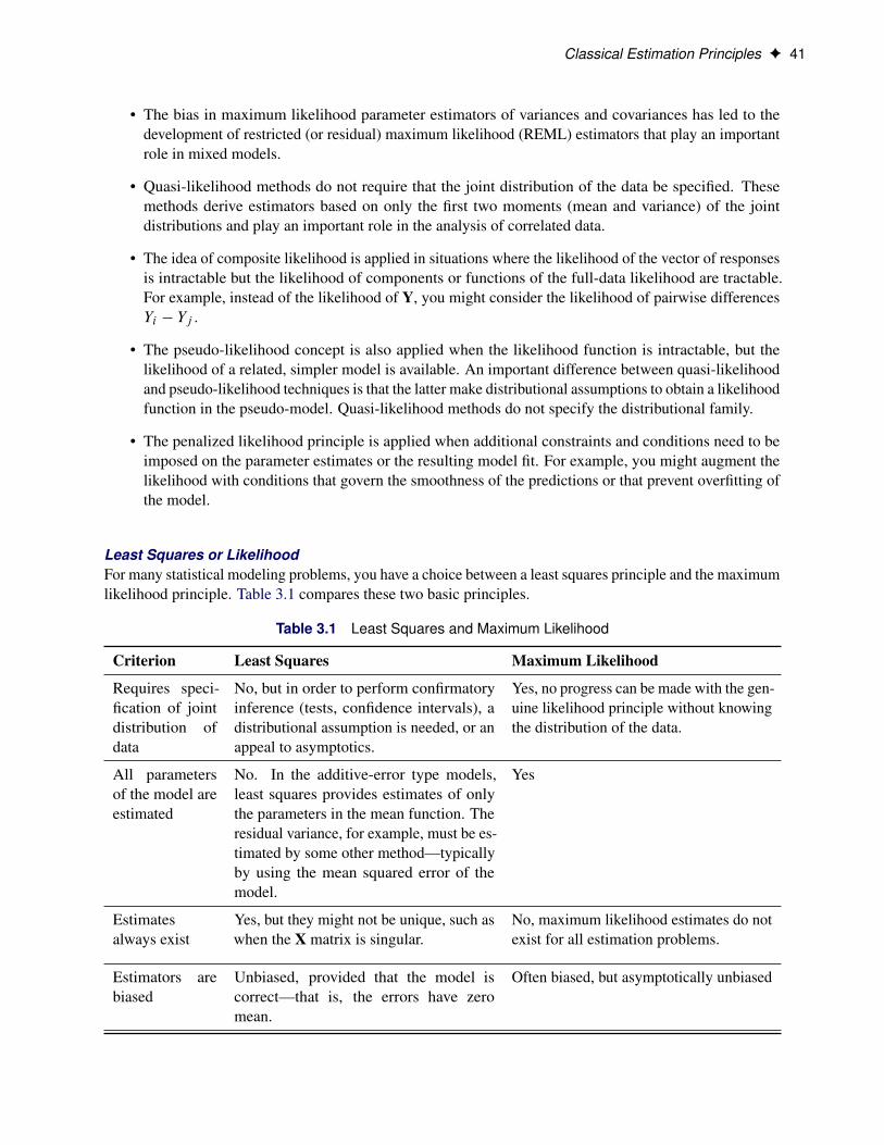
Least Squares or LikelihoodFor many statistical modeling problems, you have a choice between a least squares principle and the maximumlikelihood principle. Table 3.1 compares these two basic principles.
Table 3.1 Least Squares and Maximum Likelihood
Criterion Least Squares Maximum Likelihood
Requires speci-fication of jointdistribution ofdata
No, but in order to perform confirmatoryinference (tests, confidence intervals), adistributional assumption is needed, or anappeal to asymptotics.
Yes, no progress can be made with the gen-uine likelihood principle without knowingthe distribution of the data.
All parametersof the model areestimated
No. In the additive-error type models,least squares provides estimates of onlythe parameters in the mean function. Theresidual variance, for example, must be es-timated by some other method—typicallyby using the mean squared error of themodel.
Yes
Estimatesalways exist
Yes, but they might not be unique, such aswhen the X matrix is singular.
No, maximum likelihood estimates do notexist for all estimation problems.
Estimators arebiased
Unbiased, provided that the model iscorrect—that is, the errors have zeromean.
Often biased, but asymptotically unbiased
42 F Chapter 3: Introduction to Statistical Modeling with SAS/STAT Software
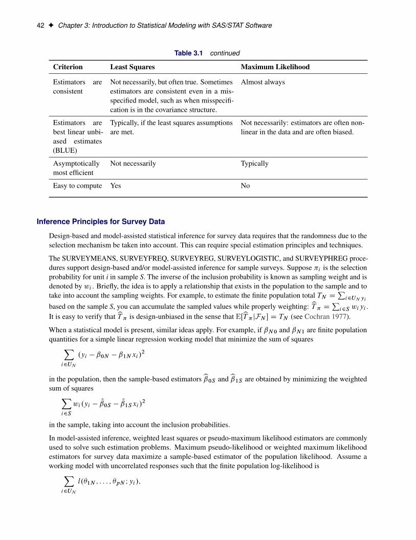
Table 3.1 continued
Criterion Least Squares Maximum Likelihood
Estimators areconsistent
Not necessarily, but often true. Sometimesestimators are consistent even in a mis-specified model, such as when misspecifi-cation is in the covariance structure.
Almost always
Estimators arebest linear unbi-ased estimates(BLUE)
Typically, if the least squares assumptionsare met.
Not necessarily: estimators are often non-linear in the data and are often biased.
Asymptoticallymost efficient
Not necessarily Typically
Easy to compute Yes No
Inference Principles for Survey Data
Design-based and model-assisted statistical inference for survey data requires that the randomness due to theselection mechanism be taken into account. This can require special estimation principles and techniques.
The SURVEYMEANS, SURVEYFREQ, SURVEYREG, SURVEYLOGISTIC, and SURVEYPHREG proce-dures support design-based and/or model-assisted inference for sample surveys. Suppose �i is the selectionprobability for unit i in sample S. The inverse of the inclusion probability is known as sampling weight and isdenoted by wi . Briefly, the idea is to apply a relationship that exists in the population to the sample and totake into account the sampling weights. For example, to estimate the finite population total TN D
Pi2UNyi
based on the sample S, you can accumulate the sampled values while properly weighting: bT � DPi2S wiyi .It is easy to verify that bT � is design-unbiased in the sense that EŒbT � jFN � D TN (see Cochran 1977).
When a statistical model is present, similar ideas apply. For example, if ˇN0 and ˇN1 are finite populationquantities for a simple linear regression working model that minimize the sum of squaresX
i2UN
.yi � ˇ0N � ˇ1Nxi /2
in the population, then the sample-based estimators b0S and b1S are obtained by minimizing the weightedsum of squaresX
i2S
wi .yi � O0S � O1Sxi /2
in the sample, taking into account the inclusion probabilities.
In model-assisted inference, weighted least squares or pseudo-maximum likelihood estimators are commonlyused to solve such estimation problems. Maximum pseudo-likelihood or weighted maximum likelihoodestimators for survey data maximize a sample-based estimator of the population likelihood. Assume aworking model with uncorrelated responses such that the finite population log-likelihood isX
i2UN
l.�1N ; : : : ; �pN Iyi /;
Statistical Background F 43
where �1N ; : : : ; �pN are finite population quantities. For independent sampling, one possible sample-basedestimator of the population log likelihood isX
i2S
wi l.�1N ; : : : ; �pN Iyi /
Sample-based estimatorsb�1S ; : : : ;b�pS are obtained by maximizing this expression.
Design-based and model-based statistical analysis might employ the same statistical model (for example, alinear regression) and the same estimation principle (for example, weighted least squares), and arrive at thesame estimates. The design-based estimation of the precision of the estimators differs from the model-basedestimation, however. For complex surveys, design-based variance estimates are in general different from theirmodel-based counterpart. The SAS/STAT procedures for survey data (SURVEYMEANS, SURVEYFREQ,SURVEYREG, SURVEYLOGISTIC, and SURVEYPHREG procedures) compute design-based varianceestimates for complex survey data. See the section “Variance Estimation” on page 251, in Chapter 14,“Introduction to Survey Procedures,” for details about design-based variance estimation.
Statistical Background
Hypothesis Testing and PowerIn statistical hypothesis testing, you typically express the belief that some effect exists in a population byspecifying an alternative hypothesis H1. You state a null hypothesis H0 as the assertion that the effect doesnot exist and attempt to gather evidence to reject H0 in favor of H1. Evidence is gathered in the form ofsample data, and a statistical test is used to assess H0. If H0 is rejected but there really is no effect, this iscalled a Type I error. The probability of a Type I error is usually designated “alpha” or ˛, and statistical testsare designed to ensure that ˛ is suitably small (for example, less than 0.05).
If there is an effect in the population but H0 is not rejected in the statistical test, then a Type II error has beencommitted. The probability of a Type II error is usually designated “beta” or ˇ. The probability 1 � ˇ ofavoiding a Type II error—that is, correctly rejecting H0 and achieving statistical significance, is called thepower of the test.
An important goal in study planning is to ensure an acceptably high level of power. Sample size plays aprominent role in power computations because the focus is often on determining a sufficient sample size toachieve a certain power, or assessing the power for a range of different sample sizes.
There are several tools available in SAS/STAT software for power and sample size analysis. PROC POWERcovers a variety of analyses such as t tests, equivalence tests, confidence intervals, binomial proportions,multiple regression, one-way ANOVA, survival analysis, logistic regression, and the Wilcoxon rank-sumtest. PROC GLMPOWER supports more complex linear models. The Power and Sample Size applicationprovides a user interface and implements many of the analyses supported in the procedures.
44 F Chapter 3: Introduction to Statistical Modeling with SAS/STAT Software
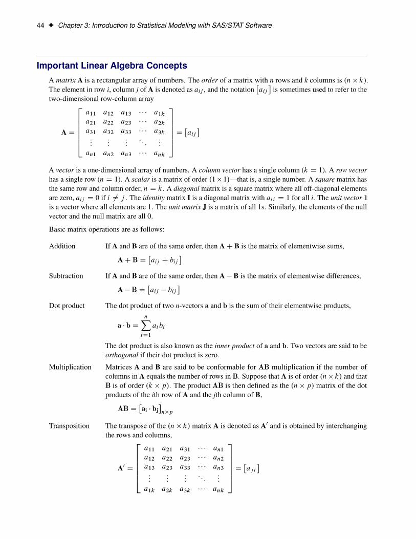
Important Linear Algebra ConceptsA matrix A is a rectangular array of numbers. The order of a matrix with n rows and k columns is .n � k/.The element in row i, column j of A is denoted as aij , and the notation
�aij�
is sometimes used to refer to thetwo-dimensional row-column array
A D
2666664a11 a12 a13 � � � a1ka21 a22 a23 � � � a2ka31 a32 a33 � � � a3k:::
::::::
: : ::::
an1 an2 an3 � � � ank
3777775 D�aij�
A vector is a one-dimensional array of numbers. A column vector has a single column (k D 1). A row vectorhas a single row (n D 1). A scalar is a matrix of order .1� 1/—that is, a single number. A square matrix hasthe same row and column order, n D k. A diagonal matrix is a square matrix where all off-diagonal elementsare zero, aij D 0 if i 6D j . The identity matrix I is a diagonal matrix with ai i D 1 for all i. The unit vector 1is a vector where all elements are 1. The unit matrix J is a matrix of all 1s. Similarly, the elements of the nullvector and the null matrix are all 0.
Basic matrix operations are as follows:
Addition If A and B are of the same order, then AC B is the matrix of elementwise sums,
AC B D�aij C bij
�Subtraction If A and B are of the same order, then A � B is the matrix of elementwise differences,
A � B D�aij � bij
�Dot product The dot product of two n-vectors a and b is the sum of their elementwise products,
a � b DnXiD1
aibi
The dot product is also known as the inner product of a and b. Two vectors are said to beorthogonal if their dot product is zero.
Multiplication Matrices A and B are said to be conformable for AB multiplication if the number ofcolumns in A equals the number of rows in B. Suppose that A is of order .n� k/ and thatB is of order .k � p/. The product AB is then defined as the .n � p/ matrix of the dotproducts of the ith row of A and the jth column of B,
AB D�ai � bj
�n�p
Transposition The transpose of the .n � k/ matrix A is denoted as A0 and is obtained by interchangingthe rows and columns,
A0 D
2666664a11 a21 a31 � � � an1a12 a22 a23 � � � an2a13 a23 a33 � � � an3:::
::::::
: : ::::
a1k a2k a3k � � � ank
3777775 D�aj i�
Important Linear Algebra Concepts F 45
A symmetric matrix is equal to its transpose, A D A0. The inner product of two .n � 1/column vectors a and b is a � b D a0b.
Matrix Inversion
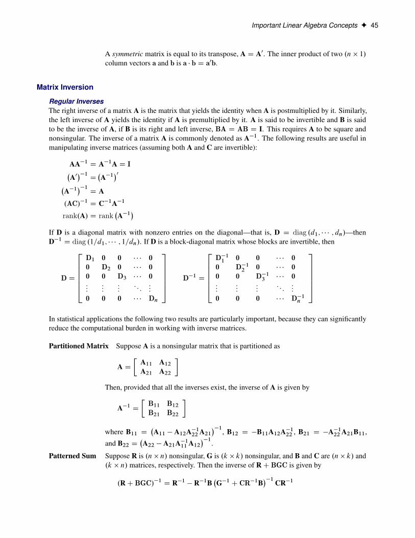
Regular InversesThe right inverse of a matrix A is the matrix that yields the identity when A is postmultiplied by it. Similarly,the left inverse of A yields the identity if A is premultiplied by it. A is said to be invertible and B is saidto be the inverse of A, if B is its right and left inverse, BA D AB D I. This requires A to be square andnonsingular. The inverse of a matrix A is commonly denoted as A�1. The following results are useful inmanipulating inverse matrices (assuming both A and C are invertible):
AA�1 D A�1A D I�A0��1D�A�1
�0�A�1
��1D A
.AC/�1 D C�1A�1
rank.A/ D rank�A�1
�If D is a diagonal matrix with nonzero entries on the diagonal—that is, D D diag .d1; � � � ; dn/—thenD�1 D diag .1=d1; � � � ; 1=dn/. If D is a block-diagonal matrix whose blocks are invertible, then
D D
2666664D1 0 0 � � � 00 D2 0 � � � 00 0 D3 � � � 0:::
::::::
: : ::::
0 0 0 � � � Dn
3777775 D�1 D
2666664D�11 0 0 � � � 00 D�12 0 � � � 00 0 D�13 � � � 0:::
::::::
: : ::::
0 0 0 � � � D�1n
3777775In statistical applications the following two results are particularly important, because they can significantlyreduce the computational burden in working with inverse matrices.
Partitioned Matrix Suppose A is a nonsingular matrix that is partitioned as
A D�
A11 A12A21 A22
�Then, provided that all the inverses exist, the inverse of A is given by
A�1 D�
B11 B12B21 B22
�where B11 D
�A11 � A12A�122A21
��1, B12 D �B11A12A�122 , B21 D �A�122A21B11,
and B22 D�A22 � A21A�111A12
��1.
Patterned Sum Suppose R is .n� n/ nonsingular, G is .k � k/ nonsingular, and B and C are .n� k/ and.k � n/ matrices, respectively. Then the inverse of RC BGC is given by
.RC BGC/�1 D R�1 � R�1B�G�1 C CR�1B
��1 CR�1
46 F Chapter 3: Introduction to Statistical Modeling with SAS/STAT Software
This formula is particularly useful if k << n and R has a simple form that is easy toinvert. This case arises, for example, in mixed models where R might be a diagonal orblock-diagonal matrix, and B D C0.Another situation where this formula plays a critical role is in the computation of regressiondiagnostics, such as in determining the effect of removing an observation from the analysis.Suppose that A D X0X represents the crossproduct matrix in the linear model EŒY� D Xˇ.If x0i is the ith row of the X matrix, then .X0X � xix0i / is the crossproduct matrix in thesame model with the ith observation removed. Identifying B D �xi , C D x0i , and G D Iin the preceding inversion formula, you can obtain the expression for the inverse of thecrossproduct matrix:
�X0X � xix0i
��1D X0XC
�X0X
��1 xix0i�X0X
��11 � x0i
�X0X
��1 xi
This expression for the inverse of the reduced data crossproduct matrix enables you tocompute “leave-one-out” deletion diagnostics in linear models without refitting the model.
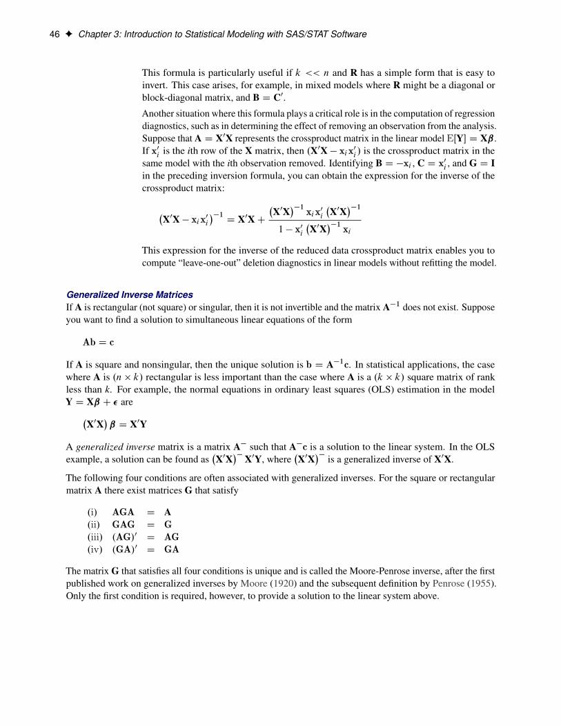
Generalized Inverse MatricesIf A is rectangular (not square) or singular, then it is not invertible and the matrix A�1 does not exist. Supposeyou want to find a solution to simultaneous linear equations of the form
Ab D c
If A is square and nonsingular, then the unique solution is b D A�1c. In statistical applications, the casewhere A is .n � k/ rectangular is less important than the case where A is a .k � k/ square matrix of rankless than k. For example, the normal equations in ordinary least squares (OLS) estimation in the modelY D Xˇ C � are�
X0X�ˇ D X0Y
A generalized inverse matrix is a matrix A� such that A�c is a solution to the linear system. In the OLSexample, a solution can be found as
�X0X
��X0Y, where�X0X
�� is a generalized inverse of X0X.
The following four conditions are often associated with generalized inverses. For the square or rectangularmatrix A there exist matrices G that satisfy
.i/ AGA D A
.ii/ GAG D G
.iii/ .AG/0 D AG
.iv/ .GA/0 D GA
The matrix G that satisfies all four conditions is unique and is called the Moore-Penrose inverse, after the firstpublished work on generalized inverses by Moore (1920) and the subsequent definition by Penrose (1955).Only the first condition is required, however, to provide a solution to the linear system above.
Important Linear Algebra Concepts F 47
Pringle and Rayner (1971) introduced a numbering system to distinguish between different types of general-ized inverses. A matrix that satisfies only condition (i) is a g1-inverse. The g2-inverse satisfies conditions (i)and (ii). It is also called a reflexive generalized inverse. Matrices satisfying conditions (i)–(iii) or conditions(i), (ii), and (iv) are g3-inverses. Note that a matrix that satisfies the first three conditions is a right generalizedinverse, and a matrix that satisfies conditions (i), (ii), and (iv) is a left generalized inverse. For example, ifB is .n � k/ of rank k, then
�B0B
��1 B0 is a left generalized inverse of B. The notation g4-inverse for theMoore-Penrose inverse, satisfying conditions (i)–(iv), is often used by extension, but note that Pringle andRayner (1971) do not use it; rather, they call such a matrix “the” generalized inverse.
If the .n � k/ matrix X is rank-deficient—that is, rank.X/ < minfn; kg—then the system of equations�X0X
�ˇ D X0Y
does not have a unique solution. A particular solution depends on the choice of the generalized inverse.However, some aspects of the statistical inference are invariant to the choice of the generalized inverse. IfG is a generalized inverse of X0X, then XGX0 is invariant to the choice of G. This result comes into play,for example, when you are computing predictions in an OLS model with a rank-deficient X matrix, since itimplies that the predicted values
XbD X�X0X
��X0y
are invariant to the choice of�X0X
��.
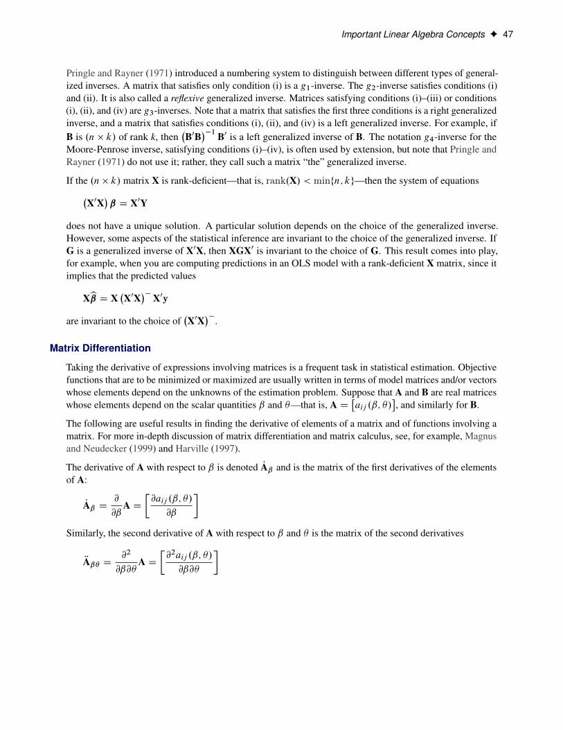
Matrix Differentiation
Taking the derivative of expressions involving matrices is a frequent task in statistical estimation. Objectivefunctions that are to be minimized or maximized are usually written in terms of model matrices and/or vectorswhose elements depend on the unknowns of the estimation problem. Suppose that A and B are real matriceswhose elements depend on the scalar quantities ˇ and �—that is, A D
�aij .ˇ; �/
�, and similarly for B.
The following are useful results in finding the derivative of elements of a matrix and of functions involving amatrix. For more in-depth discussion of matrix differentiation and matrix calculus, see, for example, Magnusand Neudecker (1999) and Harville (1997).
The derivative of A with respect to ˇ is denoted PAˇ and is the matrix of the first derivatives of the elementsof A:
PAˇ D@
@ˇA D
�@aij .ˇ; �/
@ˇ
�Similarly, the second derivative of A with respect to ˇ and � is the matrix of the second derivatives
RAˇ� D@2
@ˇ@�A D
�@2aij .ˇ; �/
@ˇ@�
�
48 F Chapter 3: Introduction to Statistical Modeling with SAS/STAT Software
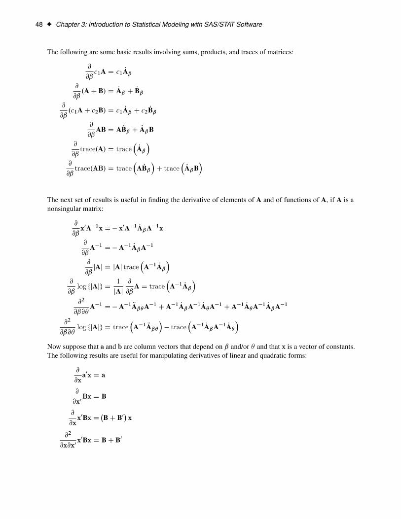
The following are some basic results involving sums, products, and traces of matrices:
@
@ˇc1A D c1 PAˇ
@
@ˇ.AC B/ D PAˇ C PBˇ
@
@ˇ.c1AC c2B/ D c1 PAˇ C c2 PBˇ
@
@ˇAB D A PBˇ C PAˇB
@
@ˇtrace.A/ D trace
�PAˇ�
@
@ˇtrace.AB/ D trace
�A PBˇ
�C trace
�PAˇB
�
The next set of results is useful in finding the derivative of elements of A and of functions of A, if A is anonsingular matrix:
@
@ˇx0A�1x D� x0A�1 PAˇA�1x
@
@ˇA�1 D� A�1 PAˇA�1
@
@ˇjAj D jAj trace
�A�1 PAˇ
�@
@ˇlog fjAjg D
1
jAj@
@ˇA D trace
�A�1 PAˇ
�@2
@ˇ@�A�1 D� A�1 RAˇ�A�1 C A�1 PAˇA�1 PA�A�1 C A�1 PA�A�1 PAˇA�1
@2
@ˇ@�log fjAjg D trace
�A�1 RAˇ�
�� trace
�A�1 PAˇA�1 PA�
�Now suppose that a and b are column vectors that depend on ˇ and/or � and that x is a vector of constants.The following results are useful for manipulating derivatives of linear and quadratic forms:
@
@xa0x D a
@
@x0Bx D B
@
@xx0Bx D
�BC B0
�x
@2
@x@x0x0Bx D BC B0
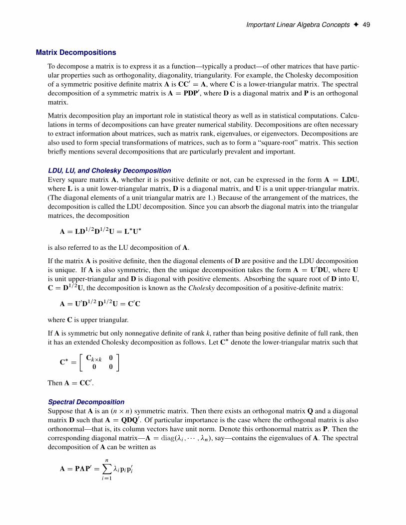
Important Linear Algebra Concepts F 49
Matrix Decompositions
To decompose a matrix is to express it as a function—typically a product—of other matrices that have partic-ular properties such as orthogonality, diagonality, triangularity. For example, the Cholesky decompositionof a symmetric positive definite matrix A is CC0 D A, where C is a lower-triangular matrix. The spectraldecomposition of a symmetric matrix is A D PDP0, where D is a diagonal matrix and P is an orthogonalmatrix.
Matrix decomposition play an important role in statistical theory as well as in statistical computations. Calcu-lations in terms of decompositions can have greater numerical stability. Decompositions are often necessaryto extract information about matrices, such as matrix rank, eigenvalues, or eigenvectors. Decompositions arealso used to form special transformations of matrices, such as to form a “square-root” matrix. This sectionbriefly mentions several decompositions that are particularly prevalent and important.
LDU, LU, and Cholesky DecompositionEvery square matrix A, whether it is positive definite or not, can be expressed in the form A D LDU,where L is a unit lower-triangular matrix, D is a diagonal matrix, and U is a unit upper-triangular matrix.(The diagonal elements of a unit triangular matrix are 1.) Because of the arrangement of the matrices, thedecomposition is called the LDU decomposition. Since you can absorb the diagonal matrix into the triangularmatrices, the decomposition
A D LD1=2D1=2U D L�U�
is also referred to as the LU decomposition of A.
If the matrix A is positive definite, then the diagonal elements of D are positive and the LDU decompositionis unique. If A is also symmetric, then the unique decomposition takes the form A D U0DU, where Uis unit upper-triangular and D is diagonal with positive elements. Absorbing the square root of D into U,C D D1=2U, the decomposition is known as the Cholesky decomposition of a positive-definite matrix:
A D U0D1=2 D1=2U D C0C
where C is upper triangular.
If A is symmetric but only nonnegative definite of rank k, rather than being positive definite of full rank, thenit has an extended Cholesky decomposition as follows. Let C� denote the lower-triangular matrix such that
C� D�
Ck�k 00 0
�Then A D CC0.
Spectral DecompositionSuppose that A is an .n � n/ symmetric matrix. Then there exists an orthogonal matrix Q and a diagonalmatrix D such that A D QDQ0. Of particular importance is the case where the orthogonal matrix is alsoorthonormal—that is, its column vectors have unit norm. Denote this orthonormal matrix as P. Then thecorresponding diagonal matrix—ƒ D diag.�i ; � � � ; �n/, say—contains the eigenvalues of A. The spectraldecomposition of A can be written as
A D PƒP0 DnXiD1
�ipip0i
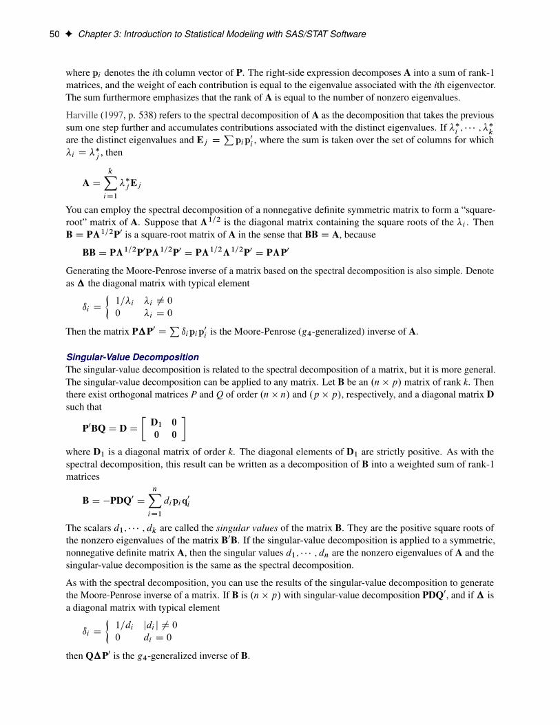
50 F Chapter 3: Introduction to Statistical Modeling with SAS/STAT Software
where pi denotes the ith column vector of P. The right-side expression decomposes A into a sum of rank-1matrices, and the weight of each contribution is equal to the eigenvalue associated with the ith eigenvector.The sum furthermore emphasizes that the rank of A is equal to the number of nonzero eigenvalues.
Harville (1997, p. 538) refers to the spectral decomposition of A as the decomposition that takes the previoussum one step further and accumulates contributions associated with the distinct eigenvalues. If ��i ; � � � ; �
�k
are the distinct eigenvalues and Ej DP
pip0i , where the sum is taken over the set of columns for which�i D �
�j , then
A DkXiD1
��jEj
You can employ the spectral decomposition of a nonnegative definite symmetric matrix to form a “square-root” matrix of A. Suppose that ƒ1=2 is the diagonal matrix containing the square roots of the �i . ThenB D Pƒ1=2P0 is a square-root matrix of A in the sense that BB D A, because
BB D Pƒ1=2P0Pƒ1=2P0 D Pƒ1=2ƒ1=2P0 D PƒP0
Generating the Moore-Penrose inverse of a matrix based on the spectral decomposition is also simple. Denoteas� the diagonal matrix with typical element
ıi D
�1=�i �i 6D 0
0 �i D 0
Then the matrix P�P0 DPıipip0i is the Moore-Penrose (g4-generalized) inverse of A.
Singular-Value DecompositionThe singular-value decomposition is related to the spectral decomposition of a matrix, but it is more general.The singular-value decomposition can be applied to any matrix. Let B be an .n � p/ matrix of rank k. Thenthere exist orthogonal matrices P and Q of order .n � n/ and .p � p/, respectively, and a diagonal matrix Dsuch that
P0BQ D D D�
D1 00 0
�where D1 is a diagonal matrix of order k. The diagonal elements of D1 are strictly positive. As with thespectral decomposition, this result can be written as a decomposition of B into a weighted sum of rank-1matrices
B D �PDQ0 DnXiD1
dipiq0i
The scalars d1; � � � ; dk are called the singular values of the matrix B. They are the positive square roots ofthe nonzero eigenvalues of the matrix B0B. If the singular-value decomposition is applied to a symmetric,nonnegative definite matrix A, then the singular values d1; � � � ; dn are the nonzero eigenvalues of A and thesingular-value decomposition is the same as the spectral decomposition.
As with the spectral decomposition, you can use the results of the singular-value decomposition to generatethe Moore-Penrose inverse of a matrix. If B is .n � p/ with singular-value decomposition PDQ0, and if� isa diagonal matrix with typical element
ıi D
�1=di jdi j 6D 0
0 di D 0
then Q�P0 is the g4-generalized inverse of B.
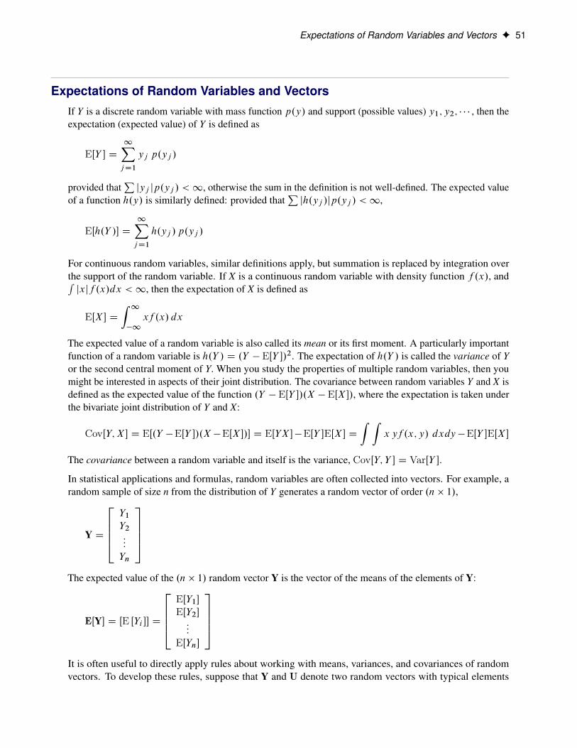
Expectations of Random Variables and Vectors F 51
Expectations of Random Variables and VectorsIf Y is a discrete random variable with mass function p.y/ and support (possible values) y1; y2; � � � , then theexpectation (expected value) of Y is defined as
EŒY � D1XjD1
yj p.yj /
provided thatPjyj jp.yj / <1, otherwise the sum in the definition is not well-defined. The expected value
of a function h.y/ is similarly defined: provided thatPjh.yj /jp.yj / <1,
EŒh.Y /� D1XjD1
h.yj / p.yj /
For continuous random variables, similar definitions apply, but summation is replaced by integration overthe support of the random variable. If X is a continuous random variable with density function f .x/, andRjxjf .x/dx <1, then the expectation of X is defined as
EŒX� DZ 1�1
xf .x/ dx
The expected value of a random variable is also called its mean or its first moment. A particularly importantfunction of a random variable is h.Y / D .Y � EŒY �/2. The expectation of h.Y / is called the variance of Yor the second central moment of Y. When you study the properties of multiple random variables, then youmight be interested in aspects of their joint distribution. The covariance between random variables Y and X isdefined as the expected value of the function .Y � EŒY �/.X � EŒX�/, where the expectation is taken underthe bivariate joint distribution of Y and X:
CovŒY; X� D EŒ.Y �EŒY �/.X �EŒX�/� D EŒYX��EŒY �EŒX� DZ Z
x yf .x; y/ dxdy�EŒY �EŒX�
The covariance between a random variable and itself is the variance, CovŒY; Y � D VarŒY �.
In statistical applications and formulas, random variables are often collected into vectors. For example, arandom sample of size n from the distribution of Y generates a random vector of order .n � 1/,
Y D
26664Y1Y2:::
Yn
37775The expected value of the .n � 1/ random vector Y is the vector of the means of the elements of Y:
EŒY� D ŒE ŒYi �� D
26664EŒY1�EŒY2�:::
EŒYn�
37775It is often useful to directly apply rules about working with means, variances, and covariances of randomvectors. To develop these rules, suppose that Y and U denote two random vectors with typical elements
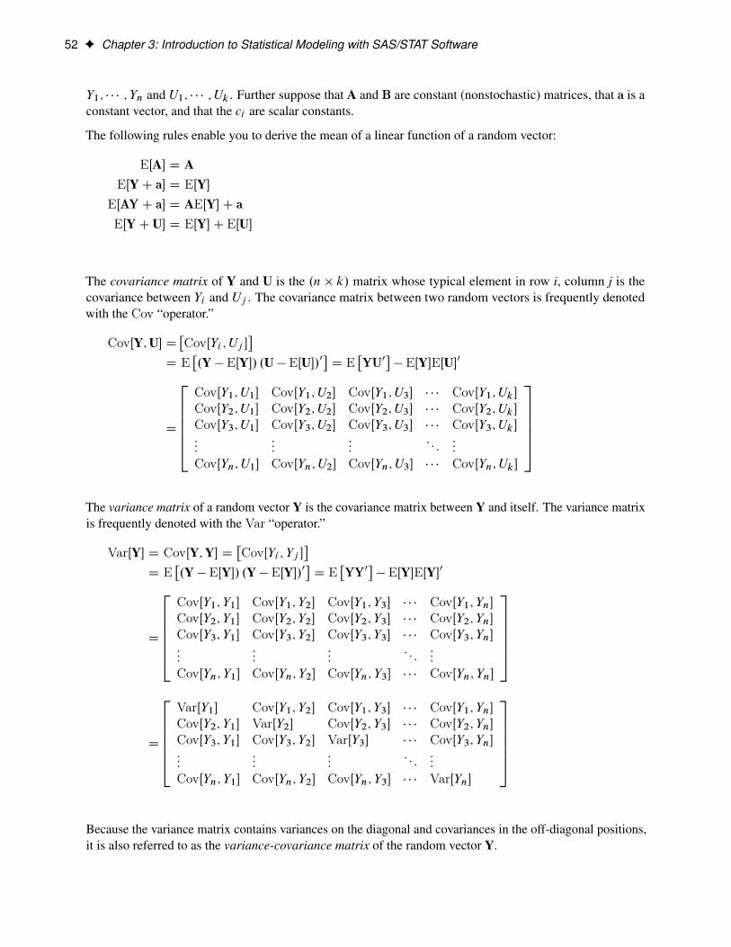
52 F Chapter 3: Introduction to Statistical Modeling with SAS/STAT Software
Y1; � � � ; Yn and U1; � � � ; Uk . Further suppose that A and B are constant (nonstochastic) matrices, that a is aconstant vector, and that the ci are scalar constants.
The following rules enable you to derive the mean of a linear function of a random vector:
EŒA� D AEŒYC a� D EŒY�
EŒAYC a� D AEŒY�C aEŒYC U� D EŒY�C EŒU�
The covariance matrix of Y and U is the .n � k/ matrix whose typical element in row i, column j is thecovariance between Yi and Uj . The covariance matrix between two random vectors is frequently denotedwith the Cov “operator.”
CovŒY;U� D�CovŒYi ; Uj �
�D E
�.Y � EŒY�/ .U � EŒU�/0
�D E
�YU0
�� EŒY�EŒU�0
D
2666664CovŒY1; U1� CovŒY1; U2� CovŒY1; U3� � � � CovŒY1; Uk�CovŒY2; U1� CovŒY2; U2� CovŒY2; U3� � � � CovŒY2; Uk�CovŒY3; U1� CovŒY3; U2� CovŒY3; U3� � � � CovŒY3; Uk�:::
::::::
: : ::::
CovŒYn; U1� CovŒYn; U2� CovŒYn; U3� � � � CovŒYn; Uk�
3777775
The variance matrix of a random vector Y is the covariance matrix between Y and itself. The variance matrixis frequently denoted with the Var “operator.”
VarŒY� D CovŒY;Y� D�CovŒYi ; Yj �
�D E
�.Y � EŒY�/ .Y � EŒY�/0
�D E
�YY0
�� EŒY�EŒY�0
D
2666664CovŒY1; Y1� CovŒY1; Y2� CovŒY1; Y3� � � � CovŒY1; Yn�CovŒY2; Y1� CovŒY2; Y2� CovŒY2; Y3� � � � CovŒY2; Yn�CovŒY3; Y1� CovŒY3; Y2� CovŒY3; Y3� � � � CovŒY3; Yn�:::
::::::
: : ::::
CovŒYn; Y1� CovŒYn; Y2� CovŒYn; Y3� � � � CovŒYn; Yn�
3777775
D
2666664VarŒY1� CovŒY1; Y2� CovŒY1; Y3� � � � CovŒY1; Yn�CovŒY2; Y1� VarŒY2� CovŒY2; Y3� � � � CovŒY2; Yn�CovŒY3; Y1� CovŒY3; Y2� VarŒY3� � � � CovŒY3; Yn�:::
::::::
: : ::::
CovŒYn; Y1� CovŒYn; Y2� CovŒYn; Y3� � � � VarŒYn�
3777775
Because the variance matrix contains variances on the diagonal and covariances in the off-diagonal positions,it is also referred to as the variance-covariance matrix of the random vector Y.
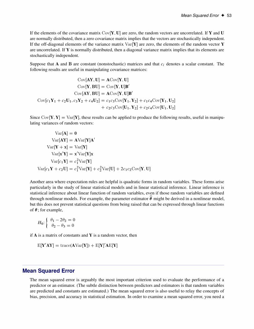
Mean Squared Error F 53
If the elements of the covariance matrix CovŒY;U� are zero, the random vectors are uncorrelated. If Y and Uare normally distributed, then a zero covariance matrix implies that the vectors are stochastically independent.If the off-diagonal elements of the variance matrix VarŒY� are zero, the elements of the random vector Yare uncorrelated. If Y is normally distributed, then a diagonal variance matrix implies that its elements arestochastically independent.
Suppose that A and B are constant (nonstochastic) matrices and that ci denotes a scalar constant. Thefollowing results are useful in manipulating covariance matrices:
CovŒAY;U� D ACovŒY;U�CovŒY;BU� D CovŒY;U�B0
CovŒAY;BU� D ACovŒY;U�B0
CovŒc1Y1 C c2U1; c3Y2 C c4U2� D c1c3CovŒY1;Y2�C c1c4CovŒY1;U2�C c2c3CovŒU1;Y2�C c2c4CovŒU1;U2�
Since CovŒY;Y� D VarŒY�, these results can be applied to produce the following results, useful in manipu-lating variances of random vectors:
VarŒA� D 0VarŒAY� D AVarŒY�A0
VarŒYC x� D VarŒY�VarŒx0Y� D x0VarŒY�x
VarŒc1Y� D c21VarŒY�
VarŒc1YC c2U� D c21VarŒY�C c22VarŒU�C 2c1c2CovŒY;U�
Another area where expectation rules are helpful is quadratic forms in random variables. These forms ariseparticularly in the study of linear statistical models and in linear statistical inference. Linear inference isstatistical inference about linear function of random variables, even if those random variables are definedthrough nonlinear models. For example, the parameter estimatorb� might be derived in a nonlinear model,but this does not prevent statistical questions from being raised that can be expressed through linear functionsof �; for example,
H0W
��1 � 2�2 D 0
�2 � �3 D 0
if A is a matrix of constants and Y is a random vector, then
EŒY0AY� D trace.AVarŒY�/C EŒY�0AEŒY�
Mean Squared ErrorThe mean squared error is arguably the most important criterion used to evaluate the performance of apredictor or an estimator. (The subtle distinction between predictors and estimators is that random variablesare predicted and constants are estimated.) The mean squared error is also useful to relay the concepts ofbias, precision, and accuracy in statistical estimation. In order to examine a mean squared error, you need a
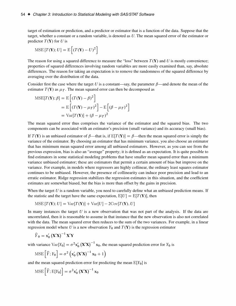
54 F Chapter 3: Introduction to Statistical Modeling with SAS/STAT Software
target of estimation or prediction, and a predictor or estimator that is a function of the data. Suppose that thetarget, whether a constant or a random variable, is denoted as U. The mean squared error of the estimator orpredictor T .Y/ for U is
MSE ŒT .Y/IU � D Eh.T .Y/ � U/2
iThe reason for using a squared difference to measure the “loss” between T .Y/ and U is mostly convenience;properties of squared differences involving random variables are more easily examined than, say, absolutedifferences. The reason for taking an expectation is to remove the randomness of the squared difference byaveraging over the distribution of the data.
Consider first the case where the target U is a constant—say, the parameter ˇ—and denote the mean of theestimator T .Y/ as �T . The mean squared error can then be decomposed as
MSEŒT .Y/Iˇ� D Eh.T .Y/ � ˇ/2
iD E
h.T .Y/ � �T /2
i� E
h.ˇ � �T /
2i
D VarŒT .Y/�C .ˇ � �T /2
The mean squared error thus comprises the variance of the estimator and the squared bias. The twocomponents can be associated with an estimator’s precision (small variance) and its accuracy (small bias).
If T .Y/ is an unbiased estimator of ˇ—that is, if EŒT .Y/� D ˇ—then the mean squared error is simply thevariance of the estimator. By choosing an estimator that has minimum variance, you also choose an estimatorthat has minimum mean squared error among all unbiased estimators. However, as you can see from theprevious expression, bias is also an “average” property; it is defined as an expectation. It is quite possible tofind estimators in some statistical modeling problems that have smaller mean squared error than a minimumvariance unbiased estimator; these are estimators that permit a certain amount of bias but improve on thevariance. For example, in models where regressors are highly collinear, the ordinary least squares estimatorcontinues to be unbiased. However, the presence of collinearity can induce poor precision and lead to anerratic estimator. Ridge regression stabilizes the regression estimates in this situation, and the coefficientestimates are somewhat biased, but the bias is more than offset by the gains in precision.
When the target U is a random variable, you need to carefully define what an unbiased prediction means. Ifthe statistic and the target have the same expectation, EŒU � D EŒT .Y/�, then
MSE ŒT .Y/IU � D VarŒT .Y/�CVarŒU � � 2CovŒT .Y/; U �
In many instances the target U is a new observation that was not part of the analysis. If the data areuncorrelated, then it is reasonable to assume in that instance that the new observation is also not correlatedwith the data. The mean squared error then reduces to the sum of the two variances. For example, in a linearregression model where U is a new observation Y0 and T .Y/ is the regression estimatorbY 0 D x00
�X0X
��1 X0Y
with variance VarŒY0� D �2x00�X0X
��1 x0, the mean squared prediction error for Y0 is
MSEhbY IY0i D �2 �x00 �X0X��1 x0 C 1
�and the mean squared prediction error for predicting the mean EŒY0� is
MSEhbY IEŒY0�i D �2x00 �X0X��1 x0
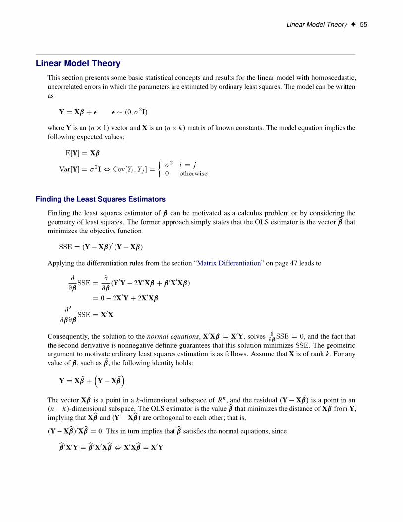
Linear Model Theory F 55
Linear Model TheoryThis section presents some basic statistical concepts and results for the linear model with homoscedastic,uncorrelated errors in which the parameters are estimated by ordinary least squares. The model can be writtenas
Y D Xˇ C � � � .0; �2I/
where Y is an .n � 1/ vector and X is an .n � k/ matrix of known constants. The model equation implies thefollowing expected values:
EŒY� D Xˇ
VarŒY� D �2I, CovŒYi ; Yj � D��2 i D j
0 otherwise
Finding the Least Squares Estimators
Finding the least squares estimator of ˇ can be motivated as a calculus problem or by considering thegeometry of least squares. The former approach simply states that the OLS estimator is the vector b thatminimizes the objective function
SSE D .Y � Xˇ/0 .Y � Xˇ/
Applying the differentiation rules from the section “Matrix Differentiation” on page 47 leads to
@
@ˇSSE D
@
@ˇ.Y0Y � 2Y0Xˇ C ˇ0X0Xˇ/
D 0 � 2X0YC 2X0Xˇ@2
@ˇ@ˇSSE D X0X
Consequently, the solution to the normal equations, X0Xˇ D X0Y, solves @@ˇ
SSE D 0, and the fact thatthe second derivative is nonnegative definite guarantees that this solution minimizes SSE. The geometricargument to motivate ordinary least squares estimation is as follows. Assume that X is of rank k. For anyvalue of ˇ, such as Q, the following identity holds:
Y D X Q C�
Y � X Q�
The vector X Q is a point in a k-dimensional subspace of Rn, and the residual .Y � X Q/ is a point in an.n � k/-dimensional subspace. The OLS estimator is the value b that minimizes the distance of X Q from Y,implying that Xb and .Y � Xb/ are orthogonal to each other; that is,
.Y � Xb/0XbD 0. This in turn implies that b satisfies the normal equations, since
b0X0Y D b0X0Xb, X0XbD X0Y
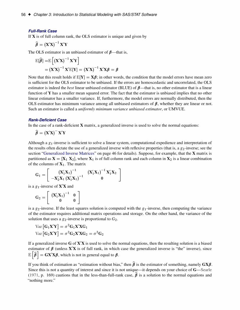
56 F Chapter 3: Introduction to Statistical Modeling with SAS/STAT Software
Full-Rank CaseIf X is of full column rank, the OLS estimator is unique and given bybD �X0X��1 X0Y
The OLS estimator is an unbiased estimator of ˇ—that is,
EŒb� DEh�
X0X��1 X0Y
iD�X0X
��1 X0EŒY� D�X0X
��1 X0Xˇ D ˇ
Note that this result holds if EŒY� D Xˇ; in other words, the condition that the model errors have mean zerois sufficient for the OLS estimator to be unbiased. If the errors are homoscedastic and uncorrelated, the OLSestimator is indeed the best linear unbiased estimator (BLUE) of ˇ—that is, no other estimator that is a linearfunction of Y has a smaller mean squared error. The fact that the estimator is unbiased implies that no otherlinear estimator has a smaller variance. If, furthermore, the model errors are normally distributed, then theOLS estimator has minimum variance among all unbiased estimators of ˇ, whether they are linear or not.Such an estimator is called a uniformly minimum variance unbiased estimator, or UMVUE.
Rank-Deficient CaseIn the case of a rank-deficient X matrix, a generalized inverse is used to solve the normal equations:bD �X0X��X0Y
Although a g1-inverse is sufficient to solve a linear system, computational expedience and interpretation ofthe results often dictate the use of a generalized inverse with reflexive properties (that is, a g2-inverse; see thesection “Generalized Inverse Matrices” on page 46 for details). Suppose, for example, that the X matrix ispartitioned as X D ŒX1 X2�, where X1 is of full column rank and each column in X2 is a linear combinationof the columns of X1. The matrix
G1 D
" �X01X1
��1 �X01X1
��1 X01X2�X02X1
�X01X1
��1 0
#is a g1-inverse of X0X and
G2 D
" �X01X1
��1 00 0
#is a g2-inverse. If the least squares solution is computed with the g1-inverse, then computing the varianceof the estimator requires additional matrix operations and storage. On the other hand, the variance of thesolution that uses a g2-inverse is proportional to G2.
Var�G1X0Y
�D �2G1X0XG1
Var�G2X0Y
�D �2G2X0XG2 D �2G2
If a generalized inverse G of X0X is used to solve the normal equations, then the resulting solution is a biasedestimator of ˇ (unless X0X is of full rank, in which case the generalized inverse is “the” inverse), sinceEhbi D GX0Xˇ, which is not in general equal to ˇ.
If you think of estimation as “estimation without bias,” then b is the estimator of something, namely GXˇ.Since this is not a quantity of interest and since it is not unique—it depends on your choice of G—Searle(1971, p. 169) cautions that in the less-than-full-rank case, b is a solution to the normal equations and“nothing more.”
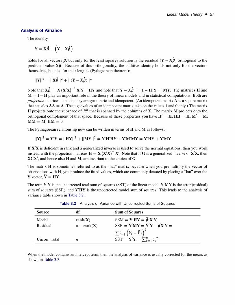
Linear Model Theory F 57
Analysis of Variance
The identity
Y D X Q C�
Y � X Q�
holds for all vectors Q, but only for the least squares solution is the residual .Y � Xb/ orthogonal to thepredicted value Xb. Because of this orthogonality, the additive identity holds not only for the vectorsthemselves, but also for their lengths (Pythagorean theorem):
jjYjj2 D jjXbjj2 C jj.Y � Xb/jj2Note that Xb D X
�X0X
��1 X0Y = HY and note that Y � Xb D .I � H/Y D MY. The matrices H andM D I �H play an important role in the theory of linear models and in statistical computations. Both areprojection matrices—that is, they are symmetric and idempotent. (An idempotent matrix A is a square matrixthat satisfies AA D A. The eigenvalues of an idempotent matrix take on the values 1 and 0 only.) The matrixH projects onto the subspace of Rn that is spanned by the columns of X. The matrix M projects onto theorthogonal complement of that space. Because of these properties you have H0 D H, HH D H, M0 D M,MM DM, HM D 0.
The Pythagorean relationship now can be written in terms of H and M as follows:
jjYjj2 D Y0Y D jjHYjj2 C jjMYjj2 D Y0H0HYC Y0M0MY D Y0HYC Y0MY
If X0X is deficient in rank and a generalized inverse is used to solve the normal equations, then you workinstead with the projection matrices H D X
�X0X
��X0. Note that if G is a generalized inverse of X0X, thenXGX0, and hence also H and M, are invariant to the choice of G.
The matrix H is sometimes referred to as the “hat” matrix because when you premultiply the vector ofobservations with H, you produce the fitted values, which are commonly denoted by placing a “hat” over theY vector, bY D HY.
The term Y0Y is the uncorrected total sum of squares (SST) of the linear model, Y0MY is the error (residual)sum of squares (SSR), and Y0HY is the uncorrected model sum of squares. This leads to the analysis ofvariance table shown in Table 3.2.
Table 3.2 Analysis of Variance with Uncorrected Sums of Squares
Source df Sum of Squares
Model rank.X/ SSM D Y0HY D b0X0YResidual n � rank.X/ SSR D Y0MY D Y0Y � bX0Y DPn
iD1
�Yi � bY i�2
Uncorr. Total n SST D Y0Y DPniD1 Y
2i
When the model contains an intercept term, then the analysis of variance is usually corrected for the mean, asshown in Table 3.3.
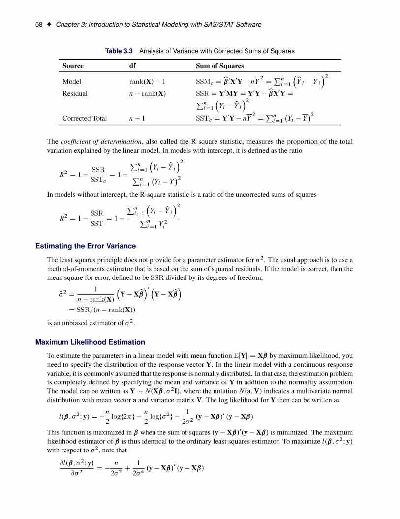
58 F Chapter 3: Introduction to Statistical Modeling with SAS/STAT Software
Table 3.3 Analysis of Variance with Corrected Sums of Squares
Source df Sum of Squares
Model rank.X/ � 1 SSMc Db0X0Y � nY 2 DPn
iD1
�bY i � Y i�2Residual n � rank.X/ SSR D Y0MY D Y0Y � bX0Y DPn
iD1
�Yi � bY i�2
Corrected Total n � 1 SSTc D Y0Y � nY 2 DPniD1
�Yi � Y
�2The coefficient of determination, also called the R-square statistic, measures the proportion of the totalvariation explained by the linear model. In models with intercept, it is defined as the ratio
R2 D 1 �SSRSSTc
D 1 �
PniD1
�Yi � bY i�2Pn
iD1
�Yi � Y
�2In models without intercept, the R-square statistic is a ratio of the uncorrected sums of squares
R2 D 1 �SSRSST
D 1 �
PniD1
�Yi � bY i�2PniD1 Y
2i
Estimating the Error Variance
The least squares principle does not provide for a parameter estimator for �2. The usual approach is to use amethod-of-moments estimator that is based on the sum of squared residuals. If the model is correct, then themean square for error, defined to be SSR divided by its degrees of freedom,
b�2 D 1
n � rank.X/
�Y � Xb�0 �Y � Xb�
D SSR=.n � rank.X//
is an unbiased estimator of �2.
Maximum Likelihood Estimation
To estimate the parameters in a linear model with mean function EŒY� D Xˇ by maximum likelihood, youneed to specify the distribution of the response vector Y. In the linear model with a continuous responsevariable, it is commonly assumed that the response is normally distributed. In that case, the estimation problemis completely defined by specifying the mean and variance of Y in addition to the normality assumption.The model can be written as Y � N.Xˇ; �2I/, where the notation N.a;V/ indicates a multivariate normaldistribution with mean vector a and variance matrix V. The log likelihood for Y then can be written as
l.ˇ; �2I y/ D �n
2logf2�g �
n
2logf�2g �
1
2�2.y � Xˇ/0 .y � Xˇ/
This function is maximized in ˇ when the sum of squares .y � Xˇ/0.y � Xˇ/ is minimized. The maximumlikelihood estimator of ˇ is thus identical to the ordinary least squares estimator. To maximize l.ˇ; �2I y/with respect to �2, note that
@l.ˇ; �2I y/@�2
D �n
2�2C
1
2�4.y � Xˇ/0 .y � Xˇ/
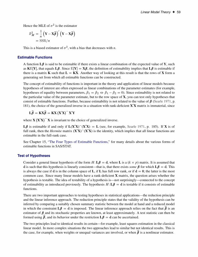
Linear Model Theory F 59
Hence the MLE of �2 is the estimator
b�2M D 1
n
�Y � Xb�0 �Y � Xb�
D SSR=n
This is a biased estimator of �2, with a bias that decreases with n.
Estimable Functions
A function Lˇ is said to be estimable if there exists a linear combination of the expected value of Y, suchas KEŒY�, that equals Lˇ. Since EŒY� D Xˇ, the definition of estimability implies that Lˇ is estimable ifthere is a matrix K such that L D KX. Another way of looking at this result is that the rows of X form agenerating set from which all estimable functions can be constructed.
The concept of estimability of functions is important in the theory and application of linear models becausehypotheses of interest are often expressed as linear combinations of the parameter estimates (for example,hypotheses of equality between parameters, ˇ1 D ˇ2, ˇ1 � ˇ2 D 0). Since estimability is not related tothe particular value of the parameter estimate, but to the row space of X, you can test only hypotheses thatconsist of estimable functions. Further, because estimability is not related to the value of ˇ (Searle 1971, p.181), the choice of the generalized inverse in a situation with rank-deficient X0X matrix is immaterial, since
LbD KXbD KX�X0X
��X0Y
where X�X0X
��X is invariant to the choice of generalized inverse.
Lˇ is estimable if and only if L.X0X/�.X0X/ D L (see, for example, Searle 1971, p. 185). If X is offull rank, then the Hermite matrix .X0X/�.X0X/ is the identity, which implies that all linear functions areestimable in the full-rank case.
See Chapter 15, “The Four Types of Estimable Functions,” for many details about the various forms ofestimable functions in SAS/STAT.
Test of Hypotheses
Consider a general linear hypothesis of the form H WLˇ D d, where L is a .k � p/ matrix. It is assumed thatd is such that this hypothesis is linearly consistent—that is, that there exists some ˇ for which Lˇ D d. Thisis always the case if d is in the column space of L, if L has full row rank, or if d D 0; the latter is the mostcommon case. Since many linear models have a rank-deficient X matrix, the question arises whether thehypothesis is testable. The idea of testability of a hypothesis is—not surprisingly—connected to the conceptof estimability as introduced previously. The hypothesis H WLˇ D d is testable if it consists of estimablefunctions.
There are two important approaches to testing hypotheses in statistical applications—the reduction principleand the linear inference approach. The reduction principle states that the validity of the hypothesis can beinferred by comparing a suitably chosen summary statistic between the model at hand and a reduced modelin which the constraint Lˇ D d is imposed. The linear inference approach relies on the fact that b is anestimator of ˇ and its stochastic properties are known, at least approximately. A test statistic can then beformed using b, and its behavior under the restriction Lˇ D d can be ascertained.
The two principles lead to identical results in certain—for example, least squares estimation in the classicallinear model. In more complex situations the two approaches lead to similar but not identical results. This isthe case, for example, when weights or unequal variances are involved, or when b is a nonlinear estimator.
60 F Chapter 3: Introduction to Statistical Modeling with SAS/STAT Software
Reduction TestsThe two main reduction principles are the sum of squares reduction test and the likelihood ratio test. The teststatistic in the former is proportional to the difference of the residual sum of squares between the reducedmodel and the full model. The test statistic in the likelihood ratio test is proportional to the difference ofthe log likelihoods between the full and reduced models. To fix these ideas, suppose that you are fitting themodel Y D Xˇ C �, where � � N.0; �2I/. Suppose that SSR denotes the residual sum of squares in thismodel and that SSRH is the residual sum of squares in the model for which Lˇ D d holds. Then under thehypothesis the ratio
.SSRH � SSR/=�2
follows a chi-square distribution with degrees of freedom equal to the rank of L. Maybe surprisingly, theresidual sum of squares in the full model is distributed independently of this quantity, so that under thehypothesis,
F D.SSRH � SSR/=rank.L/
SSR=.n � rank.X//
follows an F distribution with rank.L/ numerator and n � rank.X/ denominator degrees of freedom. Notethat the quantity in the denominator of the F statistic is a particular estimator of �2—namely, the unbiasedmoment-based estimator that is customarily associated with least squares estimation. It is also the restrictedmaximum likelihood estimator of �2 if Y is normally distributed.
In the case of the likelihood ratio test, suppose that l.b;b�2I y/ denotes the log likelihood evaluated at the MLestimators. Also suppose that l.bH ;b�2H I y/ denotes the log likelihood in the model for which Lˇ D d holds.Then under the hypothesis the statistic
� D 2�l.b;b�2I y/ � l.bH ;b�2H I y/�
follows approximately a chi-square distribution with degrees of freedom equal to the rank of L. In the case ofa normally distributed response, the log-likelihood function can be profiled with respect to ˇ. The resultingprofile log likelihood is
l.b�2I y/ D �n2
logf2�g �n
2
�logfb�2g�
and the likelihood ratio test statistic becomes
� D n�log
˚b�2H � log˚b�2� D n .log fSSRH g � log fSSRg/ D n .log fSSRH=SSRg/
The preceding expressions show that, in the case of normally distributed data, both reduction principles leadto simple functions of the residual sums of squares in two models. As Pawitan (2001, p. 151) puts it, thereis, however, an important difference not in the computations but in the statistical content. The least squaresprinciple, where sum of squares reduction tests are widely used, does not require a distributional specification.Assumptions about the distribution of the data are added to provide a framework for confirmatory inferences,such as the testing of hypotheses. This framework stems directly from the assumption about the data’sdistribution, or from the sampling distribution of the least squares estimators. The likelihood principle, onthe other hand, requires a distributional specification at the outset. Inference about the parameters is implicitin the model; it is the result of further computations following the estimation of the parameters. In the leastsquares framework, inference about the parameters is the result of further assumptions.
Linear Model Theory F 61
Linear InferenceThe principle of linear inference is to formulate a test statistic for H WLˇ D d that builds on the linearity ofthe hypothesis about ˇ. For many models that have linear components, the estimator Lb is also linear in Y.It is then simple to establish the distributional properties of Lb based on the distributional assumptions aboutY or based on large-sample arguments. For example, bmight be a nonlinear estimator, but it is known toasymptotically follow a normal distribution; this is the case in many nonlinear and generalized linear models.
If the sampling distribution or the asymptotic distribution of b is normal, then one can easily derive quadraticforms with known distributional properties. For example, if the random vector U is distributed as N.�;†/,then U0AU follows a chi-square distribution with rank.A/ degrees of freedom and noncentrality parameter1=2�0A�, provided that A†A† D A†.
In the classical linear model, suppose that X is deficient in rank and that bD �X0X��X0Y is a solution tothe normal equations. Then, if the errors are normally distributed,
b � N ��X0X
��X0Xˇ; �2�X0X
��X0X�X0X
���Because H WLˇ D d is testable, Lˇ is estimable, and thus L.X0X/�X0X D L, as established in the previoussection. Hence,
Lb � N �Lˇ; �2L
�X0X
�� L0�
The conditions for a chi-square distribution of the quadratic form
.Lb� d/0�L.X0X/�L0
��.Lb� d/
are thus met, provided that
.L.X0X/�L0/�L.X0X/�L0.L.X0X/�L0/�L.X0X/�L0 D .L.X0X/�L0/�L.X0X/�L0
This condition is obviously met if L.X0X/�L0 is of full rank. The condition is also met if L.X0X/�L0� is areflexive inverse (a g2-inverse) of L.X0X/�L.
The test statistic to test the linear hypothesis H WLˇ D d is thus
F D.Lb� d/0
�L.X0X/�L0
��.Lb� d/=rank.L/
SSR=.n � rank.X//
and it follows an F distribution with rank.L/ numerator and n � rank.X/ denominator degrees of freedomunder the hypothesis.
This test statistic looks very similar to the F statistic for the sum of squares reduction test. This is no accident.If the model is linear and parameters are estimated by ordinary least squares, then you can show that thequadratic form .Lb� d/0
�L.X0X/�L0
��.Lb� d/ equals the differences in the residual sum of squares,
SSRH � SSR, where SSRH is obtained as the residual sum of squares from OLS estimation in a model thatsatisfies Lˇ D d. However, this correspondence between the two test formulations does not apply whena different estimation principle is used. For example, assume that � � N.0;V/ and that ˇ is estimated bygeneralized least squares:
bg D
�X0V�1X
��X0V�1Y
The construction of L matrices associated with hypotheses in SAS/STAT software is frequently based onthe properties of the X matrix, not of X0V�X. In other words, the construction of the L matrix is governed
62 F Chapter 3: Introduction to Statistical Modeling with SAS/STAT Software
only by the design. A sum of squares reduction test for H WLˇ D 0 that uses the generalized residual sum ofsquares .Y � bg/0V�1.Y � bg/ is not identical to a linear hypothesis test with the statistic
F � Db0gL0
�L�X0V�1X
�� L0�� Lbg
rank.L/
Furthermore, V is usually unknown and must be estimated as well. The estimate for V depends on themodel, and imposing a constraint on the model would change the estimate. The asymptotic distribution of thestatistic F � is a chi-square distribution. However, in practical applications the F distribution with rank.L/numerator and � denominator degrees of freedom is often used because it provides a better approximation tothe sampling distribution of F � in finite samples. The computation of the denominator degrees of freedom�, however, is a matter of considerable discussion. A number of methods have been proposed and areimplemented in various forms in SAS/STAT (see, for example, the degrees-of-freedom methods in theMIXED and GLIMMIX procedures).
Residual Analysis
The model errors � D Y�Xˇ are unobservable. Yet important features of the statistical model are connectedto them, such as the distribution of the data, the correlation among observations, and the constancy ofvariance. It is customary to diagnose and investigate features of the model errors through the fitted residualsb� D Y �bY D Y �HY DMY. These residuals are projections of the data onto the null space of X and arealso referred to as the “raw” residuals to contrast them with other forms of residuals that are transformationsofb�. For the classical linear model, the statistical properties ofb� are affected by the features of that projectionand can be summarized as follows:
EŒb�� D 0
VarŒb�� D �2Mrank.M/ D n � rank.X/
Furthermore, if � � N.0; �2I/, thenb� � N.0; �2M/.
Because M D I �H, and the “hat” matrix H satisfies @bY=@Y, the hat matrix is also the leverage matrix ofthe model. If hi i denotes the ith diagonal element of H (the leverage of observation i), then the leveragesare bounded in a model with intercept, 1=n � hi i � 1. Consequently, the variance of a raw residual is lessthan that of an observation: VarŒb�i � D �2.1 � hi i / < �2. In applications where the variability of the data isestimated from fitted residuals, the estimate is invariably biased low. An example is the computation of anempirical semivariogram based on fitted (detrended) residuals.
More important, the diagonal entries of H are not necessarily identical; the residuals are heteroscedastic. The“hat” matrix is also not a diagonal matrix; the residuals are correlated. In summary, the only property that thefitted residualsb� share with the model errors is a zero mean. It is thus commonplace to use transformationsof the fitted residuals for diagnostic purposes.
Raw and Studentized ResidualsA standardized residual is a raw residual that is divided by its standard deviation:
b��i D Yi � bY iqVarŒYi � bY i � D
b�ip�2.1 � hi i /
Linear Model Theory F 63
Because �2 is unknown, residual standardization is usually not practical. A studentized residual is a rawresidual that is divided by its estimated standard deviation. If the estimate of the standard deviation is basedon the same data that were used in fitting the model, the residual is also called an internally studentizedresidual:
b�is D Yi � bY iqbVarŒYi � bY i � D
b�ipb�2.1 � hi i /If the estimate of the residual’s variance does not involve the ith observation, it is called an externallystudentized residual. Suppose thatb�2
�i denotes the estimate of the residual variance obtained without the ithobservation; then the externally studentized residual is
b�ir D b�iqb�2�i .1 � hi i /
Scaled ResidualsA scaled residual is simply a raw residual divided by a scalar quantity that is not an estimate of the varianceof the residual. For example, residuals divided by the standard deviation of the response variable are scaledand referred to as Pearson or Pearson-type residuals:
b�ic D Yi � bY iqbVarŒYi �
In generalized linear models, where the variance of an observation is a function of the mean � and possiblyof an extra scale parameter, VarŒY � D a.�/�, the Pearson residual is
b�iP D Yi �b�ipa.b�/
because the sum of the squared Pearson residuals equals the Pearson X2 statistic:
X2 D
nXiD1
b�2iPWhen the scale parameter � participates in the scaling, the residual is also referred to as a Pearson-typeresidual:
b�iP D Yi �b�ipa.b�/�
Other ResidualsYou might encounter other residuals in SAS/STAT software. A “leave-one-out” residual is the differencebetween the observed value and the residual obtained from fitting a model in which the observation inquestion did not participate. If bY i is the predicted value of the ith observation and bY i;�i is the predictedvalue if Yi is removed from the analysis, then the “leave-one-out” residual is
b�i;�i D Yi � bY i;�i
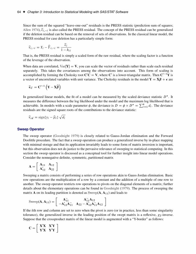
64 F Chapter 3: Introduction to Statistical Modeling with SAS/STAT Software
Since the sum of the squared “leave-one-out” residuals is the PRESS statistic (prediction sum of squares;Allen 1974),b�i;�i is also called the PRESS residual. The concept of the PRESS residual can be generalizedif the deletion residual can be based on the removal of sets of observations. In the classical linear model, thePRESS residual for case deletion has a particularly simple form:
b�i;�i D Yi � bY i;�i D b�i1 � hi i
That is, the PRESS residual is simply a scaled form of the raw residual, where the scaling factor is a functionof the leverage of the observation.
When data are correlated, VarŒY� D V, you can scale the vector of residuals rather than scale each residualseparately. This takes the covariances among the observations into account. This form of scaling isaccomplished by forming the Cholesky root C0C D V, where C0 is a lower-triangular matrix. Then C0�1Y isa vector of uncorrelated variables with unit variance. The Cholesky residuals in the model Y D Xˇ C � are
b�C D C0�1�
Y � Xb�In generalized linear models, the fit of a model can be measured by the scaled deviance statistic D�. Itmeasures the difference between the log likelihood under the model and the maximum log likelihood that isachievable. In models with a scale parameter �, the deviance is D D � �D� D
PniD1 di . The deviance
residuals are the signed square roots of the contributions to the deviance statistic:
b�id D signfyi �b�igpdiSweep Operator
The sweep operator (Goodnight 1979) is closely related to Gauss-Jordan elimination and the ForwardDoolittle procedure. The fact that a sweep operation can produce a generalized inverse by in-place mappingwith minimal storage and that its application invariably leads to some form of matrix inversion is important,but this observation does not do justice to the pervasive relevance of sweeping to statistical computing. In thissection the sweep operator is discussed as a conceptual tool for further insight into linear model operations.Consider the nonnegative definite, symmetric, partitioned matrix
A D�
A11 A12A012 A22
�Sweeping a matrix consists of performing a series of row operations akin to Gauss-Jordan elimination. Basicrow operations are the multiplication of a row by a constant and the addition of a multiple of one row toanother. The sweep operator restricts row operations to pivots on the diagonal elements of a matrix; furtherdetails about the elementary operations can be found in Goodnight (1979). The process of sweeping thematrix A on its leading partition is denoted as Sweep.A;A11/ and leads to
Sweep.A;A11/ D�
A�11 A�11A12�A012A�11 A22 � A012A�11A12
�If the kth row and column are set to zero when the pivot is zero (or in practice, less than some singularitytolerance), the generalized inverse in the leading position of the swept matrix is a reflexive, g2-inverse.Suppose that the crossproduct matrix of the linear model is augmented with a “Y-border” as follows:
C D�
X0X X0YY0X Y0Y
�
References F 65
Then the result of sweeping on the rows of X is
Sweep.C;X/ D� �
X0X�� �
X0X��X0Y
�Y0X�X0X
�� Y0Y � Y0X�X0X
��X0Y
�
D
" �X0X
�� b�b Y0MY
#D
" �X0X
�� b�b SSR
#The “Y-border” has been transformed into the least squares solution and the residual sum of squares.
Partial sweeps are common in model selection. Suppose that the X matrix is partitioned as ŒX1 X2�, andconsider the augmented crossproduct matrix
C D
24 X01X1 X01X2 X01YX02X1 X02X2 X02YY0X1 Y0X2 Y0Y
35Sweeping on the X1 partition yields
Sweep.C;X1/ D
24 �X01X1
�� �X01X1
��X01X2�X01X1
��X01Y�X02X1
�X01X1
�� X02M1X2 X02M1YY0X1
�X01X1
�� Y0M1X2 Y0M1Y
35where M1 D I � X1
�X01X1
��X01. The entries in the first row of this partition are the generalized inverseof X0X, the coefficients for regressing X2 on X1, and the coefficients for regressing Y on X1. The diagonalentries X02M1X2 and Y0M1Y are the sum of squares and crossproduct matrices for regressing X2 on X1and for regressing Y on X1, respectively. As you continue to sweep the matrix, the last cell in the partitioncontains the residual sum of square of a model in which Y is regressed on all columns swept up to that point.
The sweep operator is not only useful to conceptualize the computation of least squares solutions, Type I andType II sums of squares, and generalized inverses. It can also be used to obtain other statistical information.For example, adding the logarithms of the pivots of the rows that are swept yields the log determinant of thematrix.
References
Allen, D. M. (1974), “The Relationship between Variable Selection and Data Augmentation and a Method ofPrediction,” Technometrics, 16, 125–127.
Cochran, W. G. (1977), Sampling Techniques, 3rd Edition, New York: John Wiley & Sons.
Goodnight, J. H. (1979), “A Tutorial on the Sweep Operator,” American Statistician, 33, 149–158.
Harville, D. A. (1997), Matrix Algebra from a Statistician’s Perspective, New York: Springer-Verlag.
Hastie, T. J., Tibshirani, R. J., and Friedman, J. H. (2001), The Elements of Statistical Learning, New York:Springer-Verlag.
Jöreskog, K. G. (1973), “A General Method for Estimating a Linear Structural Equation System,” in A. S.Goldberger and O. D. Duncan, eds., Structural Equation Models in the Social Sciences, New York:Academic Press.
66 F Chapter 3: Introduction to Statistical Modeling with SAS/STAT Software
Keesling, J. W. (1972), Maximum Likelihood Approaches to Causal Analysis, Ph.D. diss., University ofChicago.
Magnus, J. R. and Neudecker, H. (1999), Matrix Differential Calculus with Applications in Statistics andEconometrics, New York: John Wiley & Sons.
McCullagh, P. and Nelder, J. A. (1989), Generalized Linear Models, 2nd Edition, London: Chapman & Hall.
Moore, E. H. (1920), “On the Reciprocal of the General Algebraic Matrix,” Bulletin of the AmericanMathematical Society, 26, 394–395.
Nelder, J. A. and Wedderburn, R. W. M. (1972), “Generalized Linear Models,” Journal of the Royal StatisticalSociety, Series A, 135, 370–384.
Pawitan, Y. (2001), In All Likelihood: Statistical Modelling and Inference Using Likelihood, Oxford:Clarendon Press.
Penrose, R. A. (1955), “A Generalized Inverse for Matrices,” Proceedings of the Cambridge PhilosophicalSociety, 51, 406–413.
Pringle, R. M. and Rayner, A. A. (1971), Generalized Inverse Matrices with Applications to Statistics, NewYork: Hafner Publishing.
Särndal, C. E., Swensson, B., and Wretman, J. (1992), Model Assisted Survey Sampling, New York: Springer-Verlag.
Searle, S. R. (1971), Linear Models, New York: John Wiley & Sons.
Spearman, C. (1904), “General Intelligence Objectively Determined and Measured,” American Journal ofPsychology, 15, 201–293.
Wedderburn, R. W. M. (1974), “Quasi-likelihood Functions, Generalized Linear Models, and the Gauss-Newton Method,” Biometrika, 61, 439–447.
Wiley, D. E. (1973), “The Identification Problem for Structural Equation Models with Unmeasured Variables,”in A. S. Goldberger and O. D. Duncan, eds., Structural Equation Models in the Social Sciences, New York:Academic Press.

Index
analysis of variancecorrected total sum of squares (Introduction to
Modeling), 57geometry (Introduction to Modeling), 57model (Introduction to Modeling), 29sum of squares (Introduction to Modeling), 29uncorrected total sum of squares (Introduction to
Modeling), 57
Bayesian modelsIntroduction to Modeling, 36
classification effectIntroduction to Modeling, 29
coefficient of determinationdefinition (Introduction to Modeling), 58
covariancematrix, definition (Introduction to Modeling), 52of random variables (Introduction to Modeling),
51
estimabilitydefinition (Introduction to Modeling), 59
estimable functiondefinition (Introduction to Modeling), 59
estimating equationsIntroduction to Modeling, 27
expected valuedefinition (Introduction to Modeling), 51of vector (Introduction to Modeling), 51
exponential familyIntroduction to Modeling, 33
functionestimable, definition (Introduction to Modeling),
59
generalized linear modelIntroduction to Modeling, 33, 61, 63, 64
heteroscedasticityIntroduction to Modeling, 62
homoscedasticityIntroduction to Modeling, 55
hypothesis testingIntroduction to Modeling, 59
indepdendentrandom variables (Introduction to Modeling), 53
inference
design-based (Introduction to Modeling), 25model-based (Introduction to Modeling), 25
Introduction to Modelingadditive error, 27analysis of variance, 29, 57augmented crossproduct matrix, 65Bayesian models, 36Cholesky decomposition, 49, 64Cholesky residual, 64classification effect, 29coefficient of determination, 58column space, 59covariance, 51covariance matrix, 52crossproduct matrix, 65curvilinear models, 28deletion residual, 64dependent variable, 26deviance residual, 64diagonal matrix, 44, 62effect genesis, 32estimable, 59estimating equations, 27expectation operator, 27expected value, 51expected value of vector, 51exponential family, 33externally studentized residual, 63fitted residual, 62fixed effect, 31fixed-effects model, 31g1-inverse, 47g2-inverse, 47, 61, 64generalized inverse, 46, 59, 65generalized least squares, 39, 61generalized linear model, 33, 61, 63, 64hat matrix, 57, 62heterocatanomic data, 30heterogeneous multivariate data, 30heteroscedasticity, 62homocatanomic data, 30homogeneous multivariate data, 30homoscedasticity, 55hypothesis testing, 59idempotent matrix, 57independent random variables, 53independent variable, 26inner product of vectors, 45

internally studentized residual, 63inverse of matrix, 45inverse of partitioned matrix, 45inverse of patterned sum of matrices, 45inverse, generalized, 46, 59, 65iteratively reweighted least squares, 39latent variable models, 33LDU decomposition, 49least squares, 37leave-one-out residual, 63levelization, 29leverage, 62, 64likelihood, 39likelihood ratio test, 60linear hypothesis, 59linear inference, 59, 61linear model theory, 55linear regression, 28link function, 33LU decomposition, 49matrix addition, 44matrix decomposition, Cholesky, 49, 64matrix decomposition, LDU, 49matrix decomposition, LU, 49matrix decomposition, singular-value, 50matrix decomposition, spectral, 49matrix decompositions, 49matrix differentiation, 47matrix dot product, 44matrix inverse, 45matrix inverse, g1, 47matrix inverse, g2, 47, 61, 64matrix inverse, Moore-Penrose, 46, 50matrix inverse, partitioned, 45matrix inverse, patterned sum, 45matrix inverse, reflexive, 47, 61, 64matrix multiplication, 44matrix order, 44matrix partition, 64matrix subtraction, 44matrix transposition, 44matrix, column space, 59matrix, diagonal, 44, 62matrix, idempotent, 57matrix, projection, 57matrix, rank deficient, 59matrix, square, 44matrix, sweeping, 64mean function, 27mean squared error, 53model fitting, 25model-based v. design-based, 25Moore-Penrose inverse, 46, 50multivariate model, 30
nonlinear model, 27, 61outcome variable, 26parameter, 24Pearson-type residual, 63power, 43PRESS statistic, 64projected residual, 62projection matrix, 57pseudo-likelihood, 39quadratic forms, 53quasi-likelihood, 39R-square, 58random effect, 31random-effects model, 31rank deficient matrix, 59raw residual, 62reduction principle, testing, 59reflexive inverse, 47, 61, 64residual analysis, 62residual, Cholesky, 64residual, deletion, 64residual, deviance, 64residual, externally studentized, 63residual, fitted, 62residual, internally studentized, 63residual, leave-one-out, 63residual, Pearson-type, 63residual, PRESS, 64residual, projected, 62residual, raw, 62residual, scaled, 63residual, standardized, 62residual, studentized, 63response variable, 26sample size, 43scaled residual, 63singular-value decomposition, 50spectral decomposition, 49square matrix, 44standardized residual, 62statistical model, 24stochastic model, 24studentized residual, 63sum of squares reduction test, 60, 61sweep, elementary operations, 64sweep, log determinant, 65sweep, operator, 64sweep, pivots, 64testable hypothesis, 59, 61testing hypotheses, 59uncorrelated random variables, 53univariate model, 30variance, 51variance matrix, 52

variance-covariance matrix, 52weighted least squares, 38
latent variable modelsIntroduction to Modeling, 33
least squaresdefinition (Introduction to Modeling), 37generalized (Introduction to Modeling), 39, 61iteratively reweighted (Introduction to Modeling),
39weighted (Introduction to Modeling), 38
likelihoodfunction (Introduction to Modeling), 40Introduction to Modeling, 39
likelihood ratio testIntroduction to Modeling, 60
linear hypothesisconsistency (Introduction to Modeling), 59definition (Introduction to Modeling), 59Introduction to Modeling, 59linear inference principle (Introduction to
Modeling), 59, 61reduction principle (Introduction to Modeling), 59testable (Introduction to Modeling), 59, 61testing (Introduction to Modeling), 59testing, linear inference (Introduction to
Modeling), 59, 61testing, reduction principle (Introduction to
Modeling), 59linear model theory
Introduction to Modeling, 55linear regression
Introduction to Modeling, 28link function
Introduction to Modeling, 33
matrixaddition (Introduction to Modeling), 44Choleksy decomposition (Introduction to
Modeling), 49, 64column space (Introduction to Modeling), 59crossproduct (Introduction to Modeling), 65crossproduct, augmented (Introduction to
Modeling), 65decomposition, Cholesky (Introduction to
Modeling), 49, 64decomposition, LDU (Introduction to Modeling),
49decomposition, LU (Introduction to Modeling),
49decomposition, singular-value (Introduction to
Modeling), 50decomposition, spectral (Introduction to
Modeling), 49
decompositions (Introduction to Modeling), 49determinant, by sweeping (Introduction to
Modeling), 65diagonal (Introduction to Modeling), 44, 62differentiation (Introduction to Modeling), 47dot product (Introduction to Modeling), 44g1-inverse (Introduction to Modeling), 47g2-inverse (Introduction to Modeling), 47, 61, 64generalized inverse (Introduction to Modeling),
46, 59, 65hat (Introduction to Modeling), 57, 62idempotent (Introduction to Modeling), 57inner product (Introduction to Modeling), 45inverse (Introduction to Modeling), 45inverse, g1 (Introduction to Modeling), 47inverse, g2 (Introduction to Modeling), 47, 61, 64inverse, generalized (Introduction to Modeling),
46, 59, 65inverse, Moore-Penrose (Introduction to
Modeling), 46, 50inverse, partitioned (Introduction to Modeling),
45inverse, patterned (Introduction to Modeling), 45inverse, reflexive (Introduction to Modeling), 47,
61, 64LDU decomposition (Introduction to Modeling),
49leverage (Introduction to Modeling), 62LU decomposition (Introduction to Modeling), 49Moore-Penrose inverse (Introduction to
Modeling), 46, 50multiplication (Introduction to Modeling), 44order (Introduction to Modeling), 44partition (Introduction to Modeling), 64projection (Introduction to Modeling), 57rank deficient (Introduction to Modeling), 59reflexive inverse (Introduction to Modeling), 47,
61, 64singular-value decomposition (Introduction to
Modeling), 50spectral decomposition (Introduction to
Modeling), 49square (Introduction to Modeling), 44subtraction (Introduction to Modeling), 44sweep (Introduction to Modeling), 64transposition (Introduction to Modeling), 44
mean functionlinear (Introduction to Modeling), 27nonlinear (Introduction to Modeling), 27
mean squared errorIntroduction to Modeling, 53
multivariate dataheterocatanomic (Introduction to Modeling), 30heterogeneous (Introduction to Modeling), 30

homocatanomic (Introduction to Modeling), 30homogeneous (Introduction to Modeling), 30
nonlinear modelIntroduction to Modeling, 27
parameterdefinition (Introduction to Modeling), 24
powerIntroduction to Modeling, 43
quadratic formsIntroduction to Modeling, 53
R-squaredefinition (Introduction to Modeling), 58
residualsCholesky (Introduction to Modeling), 64deletion (Introduction to Modeling), 64deviance (Introduction to Modeling), 64externally studentized (Introduction to Modeling),
63fitted (Introduction to Modeling), 62internally studentized (Introduction to Modeling),
63leave-one-out (Introduction to Modeling), 63Pearson-type (Introduction to Modeling), 63PRESS (Introduction to Modeling), 64projected, (Introduction to Modeling), 62raw (Introduction to Modeling), 62scaled (Introduction to Modeling), 63standardized (Introduction to Modeling), 62studentized (Introduction to Modeling), 63studentized, external (Introduction to Modeling),
63studentized, internal (Introduction to Modeling),
63
sample sizeIntroduction to Modeling, 43
statistical modeldefinition (Introduction to Modeling), 24
stochastic modeldefinition (Introduction to Modeling), 24
sum of squarescorrected total (Introduction to Modeling), 57uncorrected total (Introduction to Modeling), 57
sum of squares reduction testIntroduction to Modeling, 60, 61
Sweep operatorand generalized inverse (Introduction to
Modeling), 64and log determinant (Introduction to Modeling),
65
elementary operations (Introduction to Modeling),64
Gauss-Jordan elimination (Introduction toModeling), 64
pivots (Introduction to Modeling), 64row operations (Introduction to Modeling), 64
testable hypothesisIntroduction to Modeling, 59, 61
testing hypothesesIntroduction to Modeling, 59
uncorrelatedrandom variables (Introduction to Modeling), 53
variancematrix, definition (Introduction to Modeling), 52of random variable (Introduction to Modeling), 51
variance-covariance matrixdefinition (Introduction to Modeling), 52