Introduction to Matlab – Simulink

& their application in

Control Systems ENTC 462 - Spring 2007

Introduction

Simulink (Simulation and Link) is an extension of MATLAB by Mathworks Inc. It works with MATLAB to offer modeling, simulating, and analyzing of dynamical systems under a graphical user interface (GUI) environment. The construction of a model is simplified with click-and-drag mouse operations. Simulink includes a comprehensive block library of toolboxes for both linear and nonlinear analyses. Models are hierarchical, which allow using both top-down and bottom-up approaches. As Simulink is an integral part of MATLAB, it is easy to switch back and forth during the analysis process and thus, the user may take full advantage of features offered in both environments. This tutorial presents the basic features of Simulink and is focused on control systems.

Getting Started

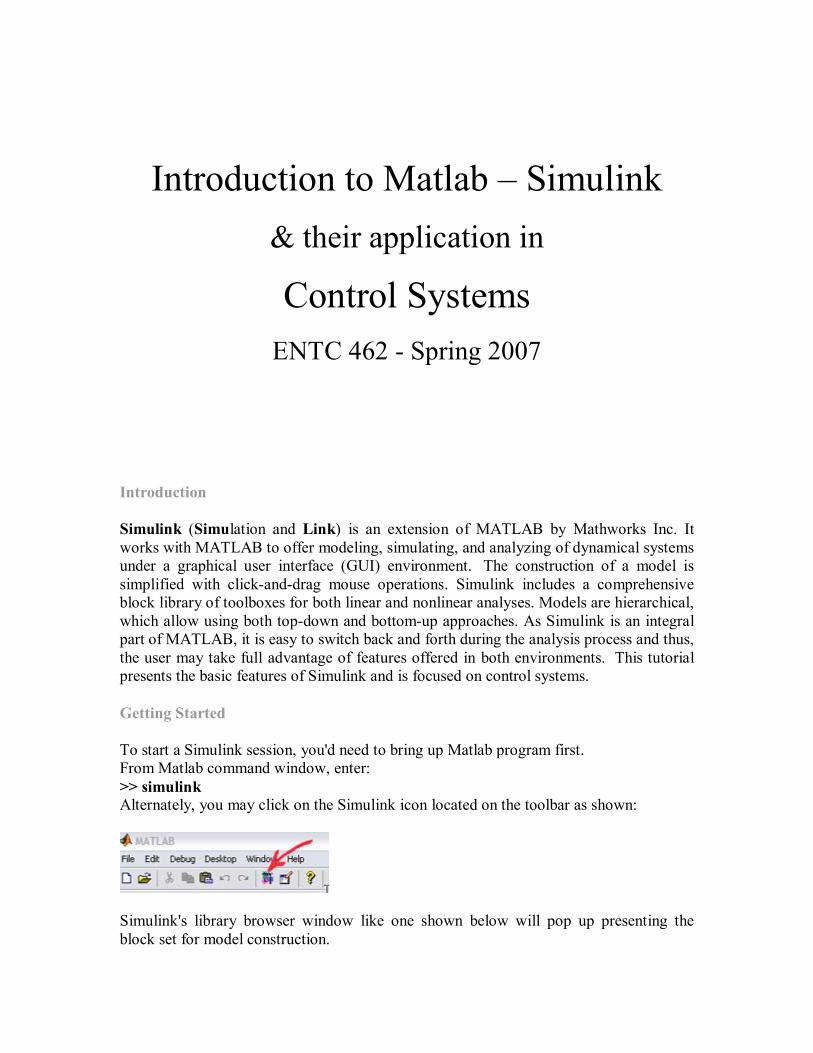
To start a Simulink session, you'd need to bring up Matlab program first. From Matlab command window, enter: >> simulink Alternately, you may click on the Simulink icon located on the toolbar as shown:

Simulink's library browser window like one shown below will pop up presenting the block set for model construction.

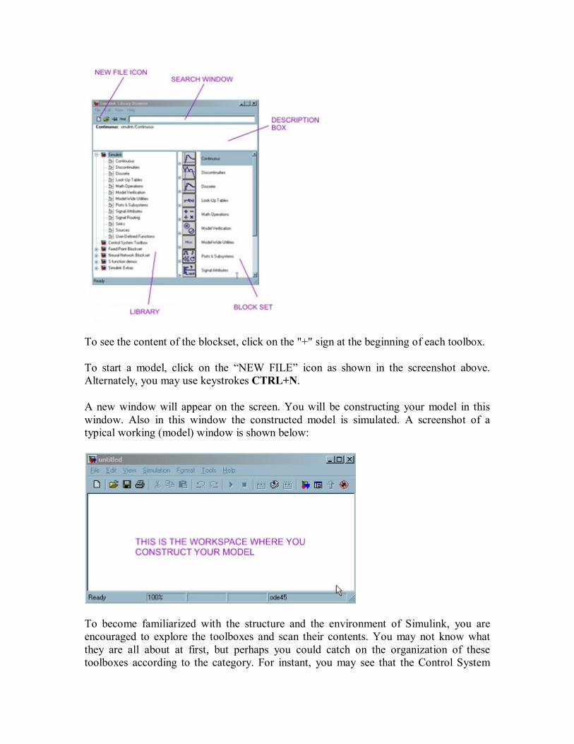
To see the content of the blockset, click on the "+" sign at the beginning of each toolbox.

To start a model, click on the “NEW FILE” icon as shown in the screenshot above. Alternately, you may use keystrokes CTRL+N.

A new window will appear on the screen. You will be constructing your model in this window. Also in this window the constructed model is simulated. A screenshot of a typical working (model) window is shown below:

To become familiarized with the structure and the environment of Simulink, you are encouraged to explore the toolboxes and scan their contents. You may not know what they are all about at first, but perhaps you could catch on the organization of these toolboxes according to the category. For instant, you may see that the Control System

toolbox consists of the Linear Time Invariant (LTI) system library and the MATLAB functions can be found under Function and Tables of the Simulink main toolbox. A good way to learn Simulink (or any computer program in general) is to practice and explore. Making mistakes is part of the learning curve. So, fear not you should be!

A simple model is used here to introduce some basic features of Simulink. Please follow the steps below to construct a simple model.

STEP 1: CREATING BLOCKS.

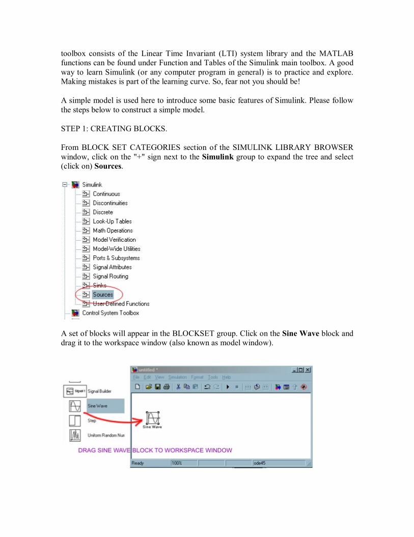
From BLOCK SET CATEGORIES section of the SIMULINK LIBRARY BROWSER window, click on the "+" sign next to the Simulink group to expand the tree and select (click on) Sources.

A set of blocks will appear in the BLOCKSET group. Click on the Sine Wave block and drag it to the workspace window (also known as model window).

Now you have established a source of your model.

NOTE: It is advisable that you save your model at some point early on so that if your PC crashes you wouldn't loose too much time reconstructing your model.

Save this model under the filename: "simexample1". To save a model, you may click on

the floppy diskette icon . or from FILE menu, select Save or CTRL+S. All Simulink model file will have an extension ".mdl". Simulink recognizes file with .mdl extension as a simulation model (similar to how MATLAB recognizes files with the extension .m as an MFile).

Continue to build your model by adding more components (or blocks) to your model window. We'll continue to add a Scope from Sinks library, an Integrator block from Continuous library, and a Mux block from Signal Routing library.

NOTE: If you wish to locate a block knowing its name, you may enter the name in the SEARCH WINDOW (at Find prompt) and Simulink will bring up the specified block.

To move the blocks around, simply click on it and drag it to a desired location.

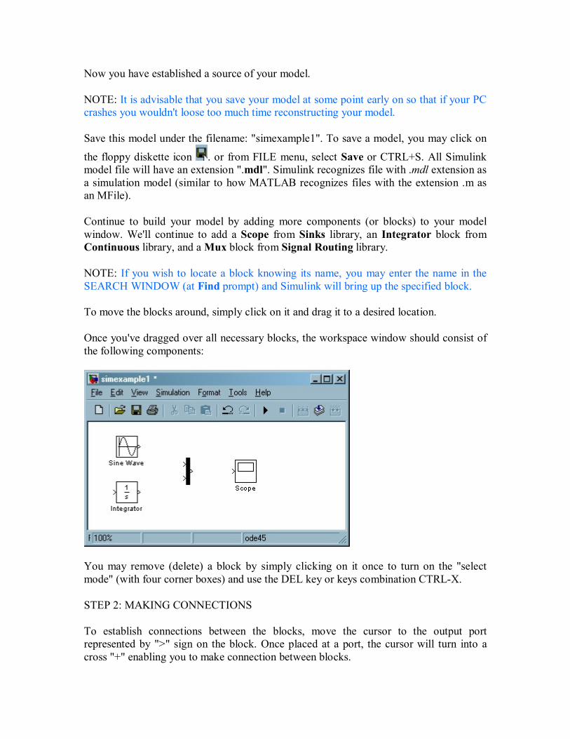
Once you've dragged over all necessary blocks, the workspace window should consist of the following components:

You may remove (delete) a block by simply clicking on it once to turn on the "select mode" (with four corner boxes) and use the DEL key or keys combination CTRL-X.

STEP 2: MAKING CONNECTIONS

To establish connections between the blocks, move the cursor to the output port represented by ">" sign on the block. Once placed at a port, the cursor will turn into a cross "+" enabling you to make connection between blocks.

To make a connection: left-click while holding down the control key (on your keyboard) and drag from source port to a destination port.

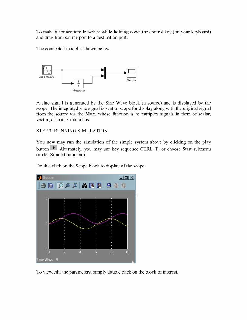
The connected model is shown below.

A sine signal is generated by the Sine Wave block (a source) and is displayed by the scope. The integrated sine signal is sent to scope for display along with the original signal from the source via the Mux, whose function is to mutiplex signals in form of scalar, vector, or matrix into a bus.

STEP 3: RUNNING SIMULATION

You now may run the simulation of the simple system above by clicking on the play button . Alternately, you may use key sequence CTRL+T, or choose Start submenu (under Simulation menu).

Double click on the Scope block to display of the scope.

To view/edit the parameters, simply double click on the block of interest.

Simulation of an Equation

In this example we will use Simulink to model an equation. Let's consider

(1)

where the displacement x is a function of time t, frequency w, phase angle phi, and amplitude A. In this example the values for these parameters are set as follows:

frequency=5 rad/sec; phase=pi/2;A=2.

where the displacement x is a function of time t, frequency w, phase angle phi, and amplitude A. In this example the values for these parameters are set as follows: frequency=5 rad/sec; phase=pi/2;A=2.

1. From Simulink library drag the following blocks to the Model Window

Blocks to be dragged to the model window

Where located in Simulink library browser

Ramp Sources Constant Sources

Gain Math Operation Sum Math Operation

Product Math Operation Trigonometry Function Math Operation

Scope Sinks Mux Signal Routing

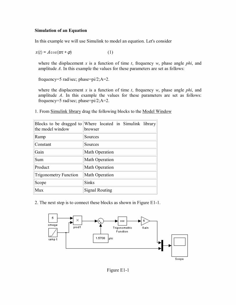
2. The next step is to connect these blocks as shown in Figure E1-1.

Figure E1-1

Double click on the blocks and enter the appropriate values as prompted by the pop-up dialog windows. Note that the cosine function can be selected from the pull-down menu in the pop-up window. In the arrangement shown above, the input signal (a ramp function) is to be displayed along with the output (displacement) via the use of the mux tool as demonstrated earlier in this tutorial. To view the plots, double click on the scope. 3. Make sure all blocks are connected correctly then run the simulation (CTRL+T). You

may need to select the Autoscale button on the scope display window to obtain a better display of the plots.

You may find the sinusoidal plots to be a bit "jaggy". You may want to improve the resolution of the displayed plot by redefining the Max Step Side value ("auto" is set a default value) in Simulation Parameters window (with keystrokes CTRL+E in the model window). Just for fun, you may want to experiment with different choice of solver. ODE45 is a default choice. You are encouraged to learn more about the solver methods by checking out the help files in Matlab command window. For instance, help ODE45 for parameters in non-stiff differential equations.

This example has demonstrated the use of Simulink with built-in mathematical functions and other supporting toolboxes to simulate an equation.

Mass-Spring-Dashpot System Simulation

Mass-Spring-Dashpot System Simulation

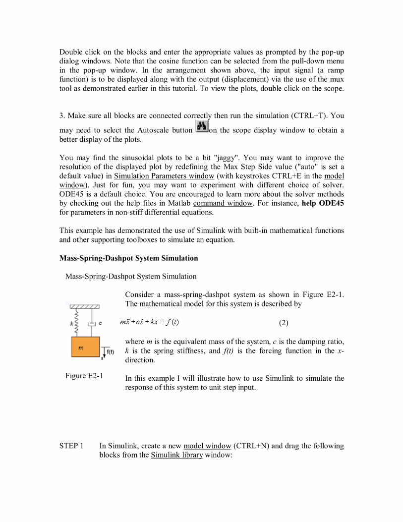
Figure E2-1

Consider a mass-spring-dashpot system as shown in Figure E2-1. The mathematical model for this system is described by

(2)

where m is the equivalent mass of the system, c is the damping ratio, k is the spring stiffness, and f(t) is the forcing function in the x-direction.

In this example I will illustrate how to use Simulink to simulate the response of this system to unit step input.

STEP 1 In Simulink, create a new model window (CTRL+N) and drag the following blocks from the Simulink library window:

Blocks to be dragged to the model window

Where located in Simulink library browser

Step Sources

Gain Math Operation Sum Math Operation

Integrator Continuous Scope Sinks

To Workspace Sinks

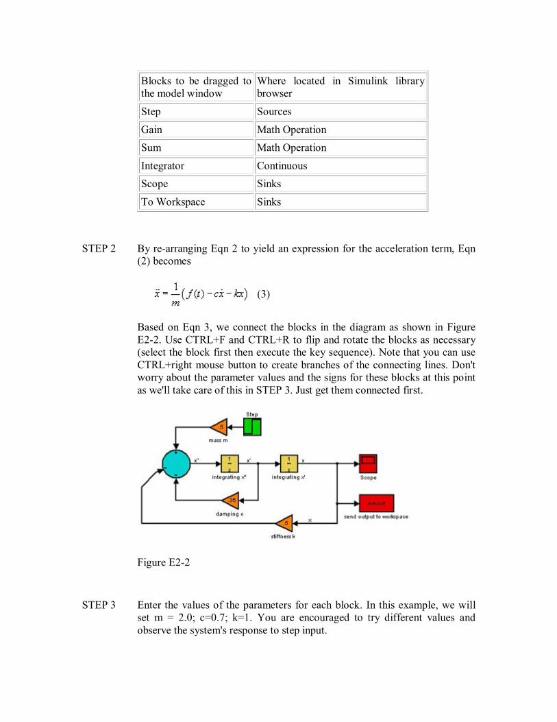
STEP 2 By re-arranging Eqn 2 to yield an expression for the acceleration term, Eqn

(2) becomes

(3)

Based on Eqn 3, we connect the blocks in the diagram as shown in Figure E2-2. Use CTRL+F and CTRL+R to flip and rotate the blocks as necessary (select the block first then execute the key sequence). Note that you can use CTRL+right mouse button to create branches of the connecting lines. Don't worry about the parameter values and the signs for these blocks at this point as we'll take care of this in STEP 3. Just get them connected first.

Figure E2-2

STEP 3 Enter the values of the parameters for each block. In this example, we will

set m = 2.0; c=0.7; k=1. You are encouraged to try different values and observe the system's response to step input.

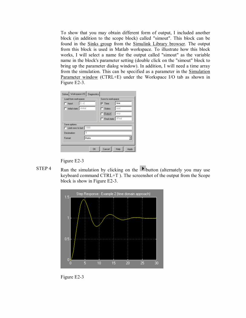
To show that you may obtain different form of output, I included another block (in addition to the scope block) called "simout". This block can be found in the Sinks group from the Simulink Library browser. The output from this block is used in Matlab workspace. To illustrate how this block works, I will select a name for the output called "simout" as the variable name in the block's parameter setting (double click on the "simout" block to bring up the parameter dialog window). In addition, I will need a time array from the simulation. This can be specified as a parameter in the Simulation Parameter window (CTRL+E) under the Workspace I/O tab as shown in Figure E2-3.

Figure E2-3 STEP 4 Run the simulation by clicking on the button (alternately you may use

keyboard command CTRL+T ). The screenshot of the output from the Scope block is show in Figure E2-3.

Figure E2-3

That's it! You have successfully modeled and simulated a second-order under-damped dynamic system. To exam different responses, feel free to change different values for m, c, and k in the gain blocks.

To see how you can use the output from the "simout" block (by the way, you may name the block whatever you wish), go to Matlab Command window and type

>> who

You should receive an echo from Matlab listing the following variables: "simout" and "time" (and perhaps others variables in the current workspace memory).

Now, you may create a plot of the system response identical to that shown in the Scope output. The command for creating this plot is:

>>plot(time,simout);grid

Note that the output format used in the example above is matrix type. The output sent to workspace can be used for further analysis and storage in ascii format. Output to workspace allows more options in plot presentation and further data analysis as the arrays are in ascii format.

The same system in transfer function

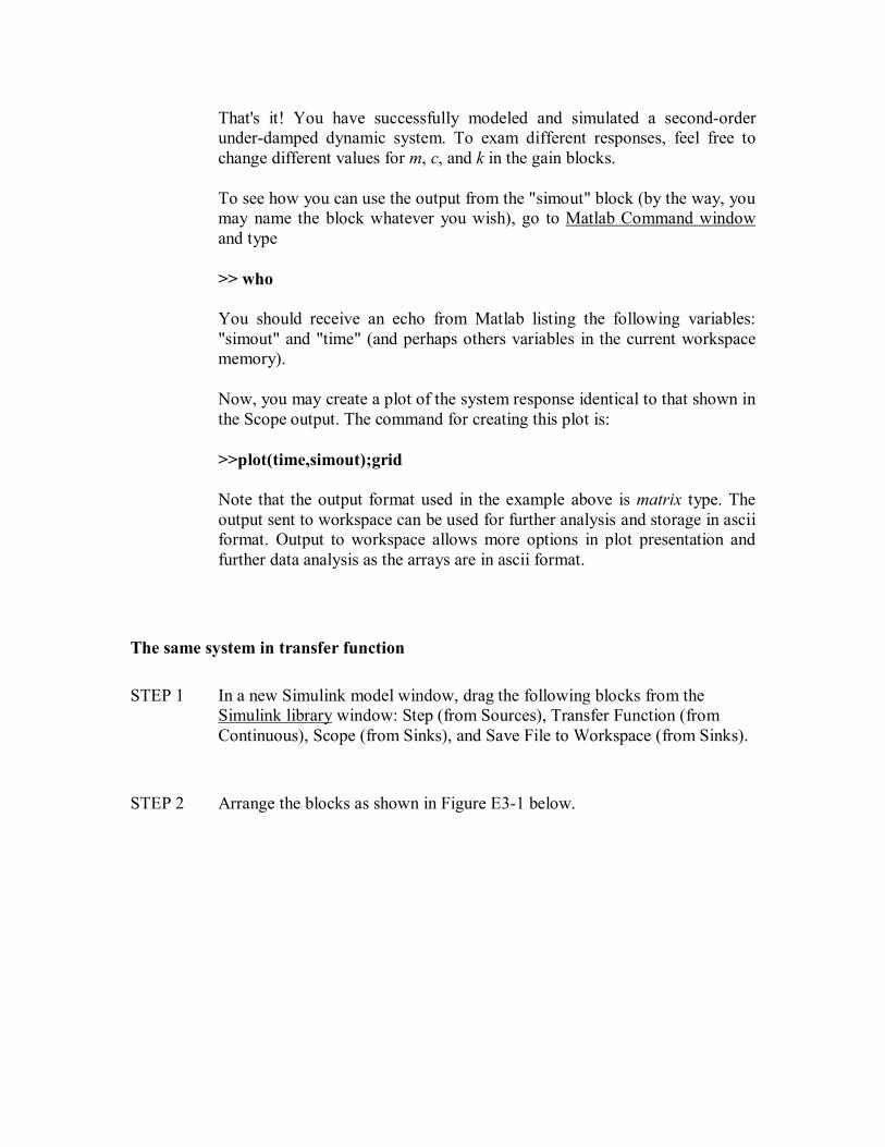
STEP 1 In a new Simulink model window, drag the following blocks from the Simulink library window: Step (from Sources), Transfer Function (from Continuous), Scope (from Sinks), and Save File to Workspace (from Sinks).

STEP 2 Arrange the blocks as shown in Figure E3-1 below.

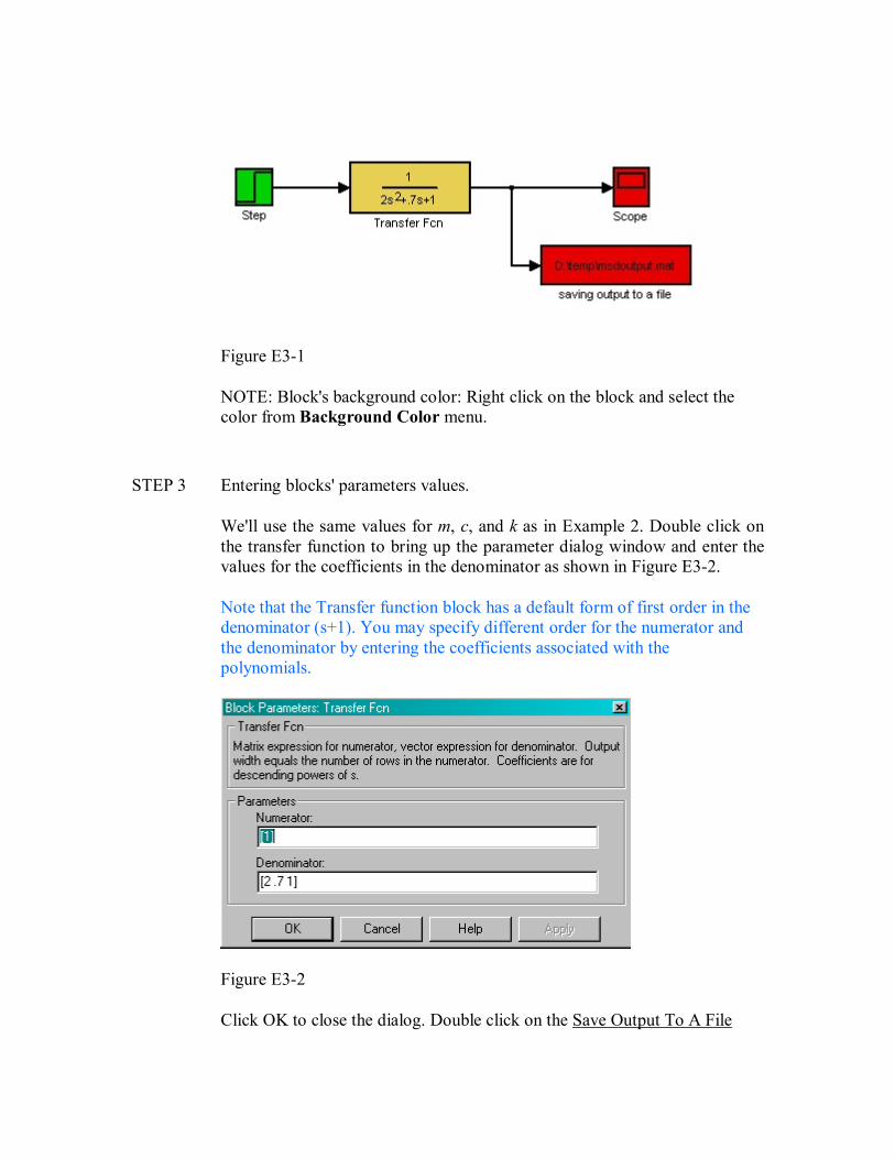
Figure E3-1

NOTE: Block's background color: Right click on the block and select the color from Background Color menu.

STEP 3 Entering blocks' parameters values.

We'll use the same values for m, c, and k as in Example 2. Double click on the transfer function to bring up the parameter dialog window and enter the values for the coefficients in the denominator as shown in Figure E3-2.

Note that the Transfer function block has a default form of first order in the denominator (s+1). You may specify different order for the numerator and the denominator by entering the coefficients associated with the polynomials.

Figure E3-2

Click OK to close the dialog. Double click on the Save Output To A File

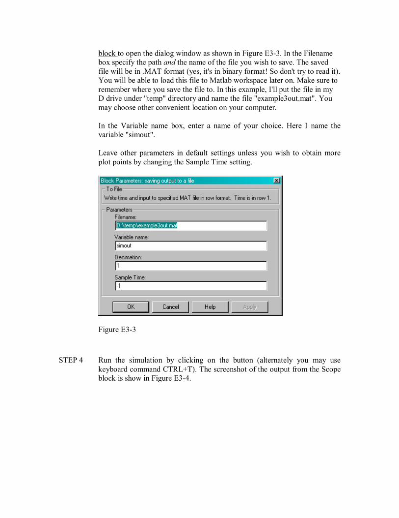
block to open the dialog window as shown in Figure E3-3. In the Filename box specify the path and the name of the file you wish to save. The saved file will be in .MAT format (yes, it's in binary format! So don't try to read it). You will be able to load this file to Matlab workspace later on. Make sure to remember where you save the file to. In this example, I'll put the file in my D drive under "temp" directory and name the file "example3out.mat". You may choose other convenient location on your computer.

In the Variable name box, enter a name of your choice. Here I name the variable "simout".

Leave other parameters in default settings unless you wish to obtain more plot points by changing the Sample Time setting.

Figure E3-3

STEP 4 Run the simulation by clicking on the button (alternately you may use

keyboard command CTRL+T). The screenshot of the output from the Scope block is show in Figure E3-4.

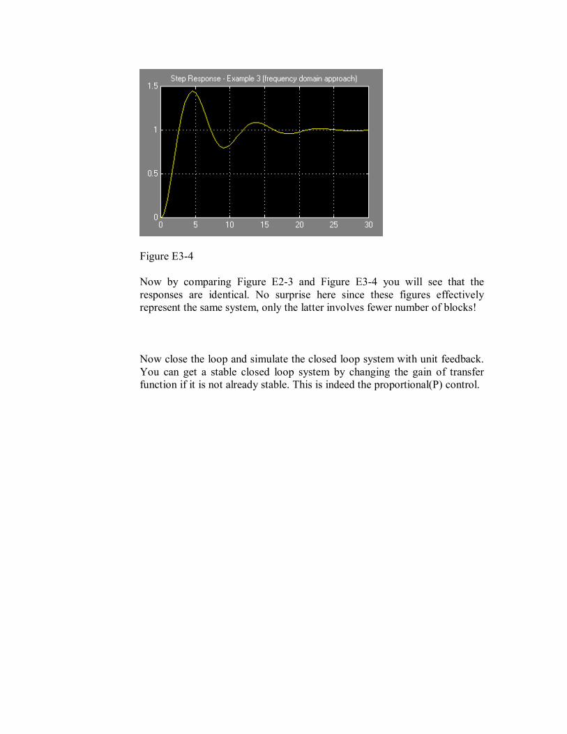
Figure E3-4

Now by comparing Figure E2-3 and Figure E3-4 you will see that the responses are identical. No surprise here since these figures effectively represent the same system, only the latter involves fewer number of blocks!

Now close the loop and simulate the closed loop system with unit feedback. You can get a stable closed loop system by changing the gain of transfer function if it is not already stable. This is indeed the proportional(P) control.