Introduction to Semidefinite Programming (SDP)

Robert M. Freund and Brian Anthony with assistance from David Craft

May 4-6, 2004

∑

∑

∑

1 Outline Slide 1

• Alternate View of Linear Programming

• Facts about Symmetric and Semidefinite Matrices

• SDP

• SDP Duality

• Examples of SDP

– Combinatorial Optimization: MAXCUT

– Convex Optimization: Quadratic Constraints, Eigenvalue Problems, log det(X) problems

• Interior-Point Methods for SDP

• Application: Truss Vibration Dynamics via SDP

2 Linear Programming

2.1 Alternative Perspective Slide 2

LP : minimize c · x

s.t. ai · x = bi, i = 1, . . . , m

n x ∈ +.

n“c · x” means the linear function “

j=1 cjxj”

n+ := x ∈ n | x ≥ 0 is the nonnegative orthant. n+ is a convex cone.

K is convex cone if x, w ∈ K and α, β ≥ 0 ⇒ αx + βw ∈ K. Slide 3

LP : minimize c · x

s.t. ai · x = bi, i = 1, . . . , m

n x ∈ +.

“Minimize the linear function c · x, subject to the condition that x must solve m given nequations ai · x = bi, i = 1, . . . , m, and that x must lie in the convex cone K = +.”

2.1.1 LP Dual Problem Slide 4

m

LD : maximize yibi

i=1 m

s.t. yiai + s = c i=1

n s ∈ +.

1

∑ ∑ ( )

∑

For feasible solutions x of LP and (y, s) of LD, the duality gap is simply

m m

c · x − yibi = c − yiai · x = s · x ≥ 0 i=1 i=1

Slide 5 ∗ ∗ ∗ If LP and LD are feasible, then there exists x and (y , s ) feasible for the primal and

dual, respectively, for which

m

∗ ∗ ∗ ∗ c · x − yi bi = s · x = 0 i=1

3 Facts about the Semidefinite Cone Slide 6

If X is an n × n matrix, then X is a symmetric positive semidefinite (SPSD) matrix if X = XT and

v T Xv ≥ 0 for any v ∈ n

If X is an n × n matrix, then X is a symmetric positive definite (SPD) matrix if X = XT and

v T Xv > 0 for any v ∈ n , v = 0

4 Facts about the Semidefinite Cone Slide 7

Sn denotes the set of symmetric n × n matrices Sn

+ denotes the set of (SPSD) n × n matrices. Sn

++ denotes the set of (SPD) n × n matrices. Let X, Y ∈ Sn . Slide 8 “X 0” denotes that X is SPSD “X Y ” denotes that X − Y 0 “X 0” to denote that X is SPD, etc. Remark: Sn = X ∈ Sn | X 0 is a convex cone. +

5 Facts about Eigenvalues and Eigenvectors Slide 9

If M is a square n × n matrix, then λ is an eigenvalue of M with corresponding eigenvector q if

Mq = λq and q = 0 .

Let λ1, λ2, . . . , λn enumerate the eigenvalues of M .

6 Facts about Eigenvalues and Eigenvectors Slide 10

2 nThe corresponding eigenvectors q 1 , q , . . . , q of M can be chosen so that they are orthonormal, namely (

i )T ( ) (

i )T ( )

jq q = 0 for i = j, and q q i = 1

2

[ ]

[ ]

∏

( )

Define: 2 nQ := q 1 q · · · q

Then Q is an orthonormal matrix:

QT −1Q = I, equivalently QT = Q

Slide 11 λ1, λ2, . . . , λn are the eigenvalues of M 1 2 n q , q , . . . , q are the corresponding orthonormal eigenvectors of M

2 nQ := q 1 q · · · q

QT Q = I, equivalently QT = Q−1

Define D: 0

λ1 0 0 λ2

D := . . . .

0 λn

Property: M = QDQT . Slide 12 The decomposition of M into M = QDQT is called its eigendecomposition.

7 Facts about Symmetric Matrices Slide 13

• If X ∈ Sn, then X = QDQT for some orthonormal matrix Q and some diagonalmatrix D. The columns of Q form a set of n orthogonal eigenvectors of X,whose eigenvalues are the corresponding entries of the diagonal matrix D.

• X 0 if and only if X = QDQT where the eigenvalues (i.e., the diagonal entriesof D) are all nonnegative.

• X 0 if and only if X = QDQT where the eigenvalues (i.e., the diagonal entriesof D) are all positive.

Slide 14

• If M is symmetric, then n

det(M) = λj

j=1

Slide 15

• Consider the matrix M defined as follows:

P v M = T v d

,

where P 0, v is a vector, and d is a scalar. Then M 0 if and only ifd − v T P−1v ≥ 0.

• For a given column vector a, the matrix X := aa T is SPSD, i.e., X = aa T 0.

• If M 0, then there is a matrix N for which M = NT N . To see this, simplytake N = D QT .

3

12

∑ ∑

( ) ( ) ( )

( )

8 SDP

8.1 Semidefinite Programming

8.1.1 Think about X Slide 16

Let X ∈ Sn . Think of X as:

• a matrix

• an array of n 2 components of the form (x11, . . . , xnn )

• an object (a vector) in the space Sn .

All three different equivalent ways of looking at X will be useful.

8.1.2 Linear Function of X Slide 17

Let X ∈ Sn . What will a linear function of X look like?If C(X) is a linear function of X, then C(X) can be written as C • X, where

n n

C • X := CijXij . i=1 j=1

There is no loss of generality in assuming that the matrix C is also symmetric.

8.1.3 Definition of SDP Slide 18

SDP : minimize C • X

s.t. Ai • X = bi , i = 1, . . . , m,

X 0,

“X 0” is the same as “X ∈ Sn ” +

The data for SDP consists of the symmetric matrix C (which is the data for the objective function) and the m symmetric matrices A1, . . . , Am, and the m−vector b, which form the m linear equations.

8.1.4 Example Slide 19 ( ) 1 2 31 0 1 0 2 8

11A1 = 0 3 7 , A2 = 2 6 0 , b = , and C = 2 9 0 ,

191 7 5 8 0 4 3 0 7

The variable X will be the 3 × 3 symmetric matrix:

x11 x12 x13

X = x21 x22 x23 , x31 x32 x33

4

( )

( )

∑

∑

∑

SDP : minimize x11 + 4x12 + 6x13 + 9x22 + 0x23 + 7x33 s.t. x11 + 0x12 + 2x13 + 3x22 + 14x23 + 5x33 = 11

0x11 + 4x12 + 16x13 + 6x22 + 0x23 + 4x33 = 19

x11 x12 x13 X = x21 x22 x23 0.

x31 x32 x33 Slide 20

SDP : minimize x11 + 4x12 + 6x13 + 9x22 + 0x23 + 7x33

s.t. x11 + 0x12 + 2x13 + 3x22 + 14x23 + 5x33 = 11 0x11 + 4x12 + 16x13 + 6x22 + 0x23 + 4x33 = 19

x11 x12 x13

X = x21 x22 x23 0. x31 x32 x33

It may be helpful to think of “X 0” as stating that each of the n eigenvalues of X must be nonnegative.

8.1.5 LP ⊂ SDP Slide 21

LP : minimize c · x s.t. ai · x = bi, i = 1, . . . , m

nx ∈ .+

Define: ai1 0 . . . 0 c1 0 . . . 0 0 ai2 . . . 0 0 c2 . . . 0

. . . .Ai = . . , i = 1, . . . , m, and C = . . . . . . . . . . . . . . . . . . . 0 0 . . . ain 0 0 . . . cn

SDP : minimize C • X s.t. Ai • X = bi , i = 1, . . . , m,

Xij = 0, i = 1, . . . , n, j = i + 1, . . . , n, x1 0 . . . 0 0 x2 . . . 0

X = . . . . 0, . . . . . . . . 0 0 . . . xn

9 SDP Duality Slide 22

m

SDD : maximize yibi

i=1

m

s.t. yiAi + S = C i=1

S 0.

Notice m

S = C − yiAi 0 i=1

5

∑

∑

( ) ( ) ( )

( ) ( ) ( )

( ) ( ) ( )

( )

∑

∑

10 SDP Duality Slide 23

and so equivalently: m

SDD : maximize yibi

i=1

m

s.t. C − yiAi 0 i=1

10.1 Example Slide 24

1 0 1 0 2 8 ( ) 1 2 3 11

A1 = 0 3 7 , A2 = 2 6 0 , b = , and C = 2 9 0 ,19

1 7 5 8 0 4 3 0 7

SDD : maximize 11y1 + 19y2

1 0 1 0 2 8 1 2 3 s.t. y1 0 3 7 + y2 2 6 0 + S = 2 9 0

1 7 5 8 0 4 3 0 7

S 0 Slide 25

SDD : maximize 11y1 + 19y2

1 0 1 0 2 8 1 2 3 s.t. y1 0 3 7 + y2 2 6 0 + S = 2 9 0

1 7 5 8 0 4 3 0 7

S 0

is the same as: SDD : maximize 11y1 + 19y2

s.t. 1 − 1y1 − 0y2 2 − 0y1 − 2y2 3 − 1y1 − 8y2

2 − 0y1 − 2y2 9 − 3y1 − 6y2 0 − 7y1 − 0y2 0. 3 − 1y1 − 8y2 0 − 7y1 − 0y2 7 − 5y1 − 4y2

10.2 Weak Duality Slide 26

Weak Duality Theorem: Given a feasible solution X of SDP and a feasible solution (y, S) of SDD, the duality gap is

m

C • X − yibi = S • X ≥ 0 . i=1

If m

C • X − yibi = 0 , i=1

then X and (y, S) are each optimal solutions to SDP and SDD, respectively, and furthermore, SX = 0.

6

∑ ∑

∑ ∑

10.3 Strong Duality Slide 27 ∗ ∗ Strong Duality Theorem: Let z and zD denote the optimal objective function

values of SDP and SDD, respectively. Suppose that there exists a feasible solution ˆ ˆ y, S) of SDD

P

X of SDP such that X 0, and that there exists a feasible solution (ˆsuch that S 0. Then both SDP and SDD attain their optimal values, and

∗ ∗ zP = zD .

11 Some Important Weaknesses of SDP Slide 28

• There may be a finite or infinite duality gap.

• The primal and/or dual may or may not attain their optima.

• Both programs will attain their common optimal value if both programs havefeasible solutions that are SPD.

• There is no finite algorithm for solving SDP .

• There is a simplex algorithm, but it is not a finite algorithm. There is no directanalog of a “basic feasible solution” for SDP .

12 SDP in Combinatorial Optimization

12.0.1 The MAX CUT Problem Slide 29

G is an undirected graph with nodes N = 1, . . . , n and edge set E.Let wij = wji be the weight on edge (i, j), for (i, j) ∈ E.We assume that wij ≥ 0 for all (i, j) ∈ E.The MAX CUT problem is to determine a subset S of the nodes N for which the

¯sum of the weights of the edges that cross from S to its complement S is maximized (S := N \ S).

12.0.2 Formulations Slide 30

The MAX CUT problem is to determine a subset S of the nodes N for which the sum ¯of the weights wij of the edges that cross from S to its complement S is maximized

(S := N \ S).Let xj = 1 for j ∈ S and xj = −1 for j ∈ S.

n n 1MAXCUT : maximizex 4

wij(1 − xixj)i=1 j=1

s.t. xj ∈ −1, 1, j = 1, . . . , n. Slide 31

n n

MAXCUT : maximizex 1 wij(1 − xixj)4

i=1 j=1

s.t. xj ∈ −1, 1, j = 1, . . . , n.

7

∑ ∑

∑ ∑

∑ ∑

∑ ∑

∑ ∑

Let Y = xx T .

Then Yij = xixj i = 1, . . . , n, j = 1, . . . , n.

Slide 32 Also let W be the matrix whose (i, j)th element is wij for i = 1, . . . , n and j = 1, . . . , n. Then

n n 1MAXCUT : maximizeY,x 4

wij − W • Yi=1 j=1

s.t. xj ∈ −1, 1, j = 1, . . . , n

Y = xx T . Slide 33

n n 1MAXCUT : maximizeY,x 4

wij − W • Yi=1 j=1

s.t. xj ∈ −1, 1, j = 1, . . . , n

Y = xx T . Slide 34

The first set of constraints are equivalent to Yjj = 1, j = 1, . . . , n.

n n 1MAXCUT : maximizeY,x 4

wij − W • Y i=1 j=1

s.t. Yjj = 1, j = 1, . . . , n

Y = xx T . Slide 35

n n 1MAXCUT : maximizeY,x 4

wij − W • Y i=1 j=1

s.t. Yjj = 1, j = 1, . . . , n

Y = xx T .

Notice that the matrix Y = xx T is a rank-1 SPSD matrix. Slide 36 We relax this condition by removing the rank-1 restriction:

n n

RELAX : maximizeY 1 wij − W • Y4

i=1 j=1

s.t. Yjj = 1, j = 1, . . . , n

Y 0.

It is therefore easy to see that RELAX provides an upper bound on MAXCUT, i.e.,

8

∑ ∑

( )

MAXCUT ≤ RELAX.

Slide 37

n n

RELAX : maximizeY 1 wij − W • Y4

i=1 j=1

s.t. Yjj = 1, j = 1, . . . , n

Y 0.

As it turns out, one can also prove without too much effort that:

0.87856 RELAX ≤ MAXCUT ≤ RELAX.

Slide 38 This is an impressive result, in that it states that the value of the semidefinite relaxation is guaranteed to be no more than 12.2% higher than the value of NP -hard problem MAX CUT.

13 SDP for Convex QCQP Slide 39

A convex quadratically constrained quadratic program (QCQP) is a problem of the form:

TQCQP : minimize x T Q0x + q0 x + c0

xTs.t. x Qix + qi

T x + ci ≤ 0 , i = 1, . . . , m,

where the Q0 0 and Qi 0, i = 1, . . . , m. This is the same as:

QCQP : minimize θx, θ

T Ts.t. x Q0x + q0 x + c0 − θ ≤ 0

T x Qix + qiT x + ci ≤ 0 , i = 1, . . . , m.

Slide 40

QCQP : minimize θx, θ

T Ts.t. x Q0x + q0 x + c0 − θ ≤ 0

T x Qix + qiT x + ci ≤ 0 , i = 1, . . . , m.

Factor each Qi into Qi = Mi

T Mi

and note the equivalence:

I Mix T

x T MiT − ci − qi

T x 0 ⇐⇒ x Qix + qi

T x + ci ≤ 0.

Slide 41

9

( )

( )

( )

( ) ( )

( )

( )

QCQP : minimize θx, θ

Ts.t. xT Q0x + q0 x + c0 − θ ≤ 0

TxT Qix + qi x + ci ≤ 0 , i = 1, . . . , m.

Re-write QCQP as:

QCQP : minimize θ x, θ

I M0x s.t. TxT MT −c0 − q0 x + θ

0 0

I Mix xT MT −ci − qi

T x 0 , i = 1, . . . , m.

i

14 SDP for SOCP

14.1 Second-Order Cone Optimization Slide 42

Second-order cone optimization:

SOCP : minx c T x

s.t. Ax = b

‖Qix + di‖ ≤ giT x + hi , i = 1, . . . , k .

√ Recall ‖v‖ := vT v Slide 43

SOCP : minx cT x

s.t. Ax = b

‖Qix + di‖ ≤ giT x + hi , i = 1, . . . , k .

Property: ( ) x + h)I (Qx + d)‖Qx + d‖ ≤ g T x + h ⇐⇒ (gT

T(Qx + d)T g x + h 0 .

This property is a direct consequence of the fact that

M = P T

v 0 ⇐⇒ d − v T P−1 v ≥ 0 . v d

Slide 44

SOCP : minx cT x

s.t. Ax = b

‖Qix + di‖ ≤ giT x + hi , i = 1, . . . , k .

Re-write as:

10

( )

∑

∑

SDPSOCP : minx cT x

s.t. Ax = b

(giT x + hi)I (Qix + di)

(Qix + di)T gi

T x + hi 0 , i = 1, . . . , k .

15 Eigenvalue Optimization Slide 45

We are given symmetric matrices B and Ai, i = 1, . . . , k Choose weights w1, . . . , wk to create a new matrix S:

k

S := B − wiAi . i=1

There might be restrictions on the weights Gw ≤ d.The typical goal is for S is to have some nice property such as:

• λmin(S) is maximized

• λmax(S) is minimized

• λmax(S) − λmin(S) is minimized

15.1 SomeUseful Relationships Slide 46

Property: M tI if and only if λmin(M) ≥ t.

Proof: M = QDQT . Define

TR = M − tI = QDQT − tI = Q(D − tI)Q .

M tI ⇐⇒ R 0 ⇐⇒ D − tI 0 ⇐⇒ λmin(M) ≥ t .

q.e.d.

Property: M tI if and only if λmax(M) ≤ t.

15.2 Design Problem Slide 47

Consider the design problem:

EOP : minimize λmax(S) − λmin(S) w, S

k

s.t. S = B − wiAi

i=1

Gw ≤ d .

Slide 48

11

∑

∑

∑ ∏ ( )

∑ ∏ ( )

( ) ( )

∑

EOP : minimize λmax(S) − λmin(S) w, S

k

s.t. S = B − wiAi

i=1

Gw ≤ d .

This is equivalent to:

EOP : minimize µ − λw, S, µ, λ

k

s.t. S = B − wiAi

i=1

Gw ≤ d λI S µI.

16 The Logarithmic Barrier Function for SPD

Matrices Slide 49

Let X 0, equivalently X ∈ Sn +.

X will have n nonnegative eigenvalues, say λ1(X), . . . , λn(X) ≥ 0 (possibly counting multiplicities).

∂Sn = X ∈ Sn | λj(X) ≥ 0, j = 1, . . . , n, +

and λj(X) = 0 for some j ∈ 1, . . . , n. Slide 50

∂Sn = X ∈ Sn | λj(X) ≥ 0, j = 1, . . . , n, +

and λj(X) = 0 for some j ∈ 1, . . . , n. A natural barrier function is:

n n

B(X) := − ln(λi(X)) = − ln λi(X) = − ln(det(X)). j=1 j=1

This function is called the log-determinant function or the logarithmic barrier function for the semidefinite cone. Slide 51

n n

B(X) := − ln(λi(X)) = − ln λi(X) = − ln(det(X)). j=1 j=1

¯Quadratic Taylor expansion at X = X:

1 ¯α2 X− 12 D X− 1

2 • X− 12 D X− 1

2 . ¯ ¯X + αD) ≈ B(X) + αX−1¯B( • D + 2

B(X) has the same remarkable properties in the context of interior-point methods for n

SDP as the barrier function − j=1

ln(xj) does in the context of linear optimization.

12

∑

∏

∑

∏

∑

∑

∑

17 The SDP Analytic Center Problem Slide 52

Given a system:

m

yiAi C ,

i=1

y, S) of: the analytic center is the solution (ˆ ˆ

n

(ACP:) maximizey,S λi(S) i=1

m s.t.

i=1 yiAi + S = C

S 0 . Slide 53

n

(ACP:) maximizey,S λi(S) i=1

m s.t.

i=1 yiAi + S = C

S 0 .

This is the same as:

(ACP:) minimizey,S − ln det(S)

m s.t.

i=1 yiAi + S = C

S 0 . Slide 54

(ACP:) minimizey,S − ln det(S)

m s.t.

i=1 yiAi + S = C

S 0 .

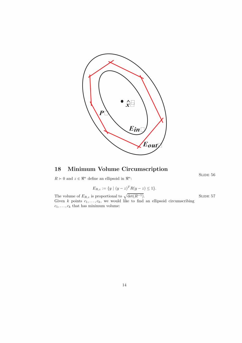
Let (y, S) be the analytic center. There are easy-to-construct ellipsoids EIN and EOUT, both centered at y and where EOUT is a scaled version of EIN with scale factor n, with the property that:

EIN ⊂ P ⊂ EOUT

Slide 55

13

√

x P

Eout

Ein

18 Minimum Volume Circumscription Slide 56

R 0 and z ∈ n define an ellipsoid in n:

ER,z := y | (y − z)T R(y − z) ≤ 1. The volume of ER,z is proportional to det(R−1). Slide 57 Given k points c1, . . . , ck, we would like to find an ellipsoid circumscribing c1, . . . , ck that has minimum volume:

14

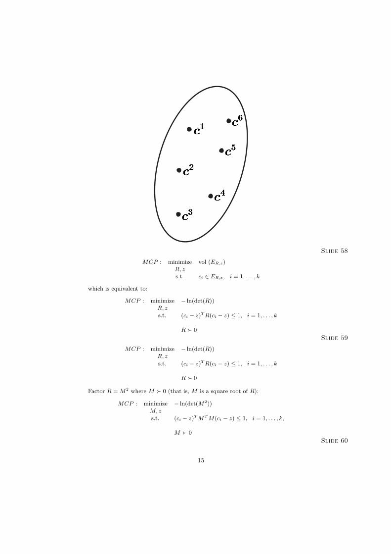
Slide 58

MCP : minimize vol (ER,z ) R, z s.t. ci ∈ ER,z , i = 1, . . . , k

which is equivalent to:

MCP : minimize − ln(det(R)) R, z s.t. (ci − z)T R(ci − z) ≤ 1, i = 1, . . . , k

R 0 Slide 59

MCP : minimize − ln(det(R)) R, z s.t. (ci − z)T R(ci − z) ≤ 1, i = 1, . . . , k

R 0

Factor R = M2 where M 0 (that is, M is a square root of R):

MCP : minimize − ln(det(M2)) M, z s.t. (ci − z)T MT M(ci − z) ≤ 1, i = 1, . . . , k,

M 0 Slide 60

15

( )

( )

( )

( )

( )

I

MCP : minimize − ln(det(M2))M, zs.t. (ci − z)T MT M(ci − z) ≤ 1, i = 1, . . . , k,

M 0.

Notice the equivalence:

Mci − Mz (Mci − Mz)T 1

0 ⇐⇒ (ci − z)T MT M(ci − z) ≤ 1

Re-write MCP :

MCP : minimize − 2 ln(det(M))M, z

I Mci − Mz s.t.

(Mci − Mz)T 1 0, i = 1, . . . , k,

M 0. Slide 61

MCP : minimize − 2 ln(det(M))M, z

I Mci − Mz s.t.

(Mci − Mz)T 1 0, i = 1, . . . , k,

M 0.

Substitute y = Mz:

MCP : minimize − 2 ln(det(M))M, y

I Mci − ys.t.

(Mci − y)T 1 0, i = 1, . . . , k,

M 0. Slide 62

MCP : minimize −2 ln(det(M))M, y

I Mci − ys.t.

(Mci − y)T 1 0, i = 1, . . . , k,

M 0.

This problem is very easy to solve.Recover the original solution R, z by computing:

R = M2 and z = M−1 y.

19 SDP in Control Theory Slide 63

A variety of control and system problems can be cast and solved as instances of SDP . This topic is beyond the scope of this lecturer’s expertise.

16

∑

∑

∑

∑ ∏ ( )

∑

20 Interior-p oint Methods for SDP

20.1 Primal and Dual SDP Slide 64

SDP : minimize C • X s.t. Ai • X = bi , i = 1, . . . , m,

X 0

and m

SDD : maximize yibi

i=1 m

s.t. yiAi + S = C i=1

S 0 .

If X and (y, S) are feasible for the primal and the dual, the duality gap is:

m

C • X − yibi = S • X ≥ 0 .

i=1

Also, S • X = 0 ⇐⇒ SX = 0 .

Slide 65

n n

B(X) = − ln(λi(X)) = − ln λi(X) = − ln(det(X)) .

j=1 j=1

Consider:

BSDP (µ) : minimize C • X − µ ln(det(X))

s.t. Ai • X = bi , i = 1, . . . , m,

X 0.

Let fµ(X) denote the objective function of BSDP (µ). Then:

−∇ fµ(X) = C − µX−1

Slide 66

BSDP (µ) : minimize C • X − µ ln(det(X))

s.t. Ai • X = bi , i = 1, . . . , m,

X 0.

∇ fµ(X) = C − µX−1

Karush-Kuhn-Tucker conditions for BSDP (µ) are: Ai • X = bi , i = 1, . . . , m, X 0, m C − µX−1 = yiAi.

i=1 Slide 67

17

∑

∑

∑ ∑ ∑ ∑

∑

Ai • X = bi , i = 1, . . . , m, X 0,

m C − µX−1 = ∑

yiAi. i=1

Define S = µX−1 ,

which implies XS = µI ,

and rewrite KKT conditions as: Slide 68 Ai • X = bi , i = 1, . . . , m, X 0 m

yiAi + S = C

i=1 XS = µI.

Slide 69 Ai • X = bi , i = 1, . . . , m, X 0 m

yiAi + S = C

i=1 XS = µI.

If (X, y, S) is a solution of this system, then X is feasible for SDP , (y, S) is feasible for SDD, and the resulting duality gap is

n n n n

S • X = SijXij = (SX)jj = (µI)jj = nµ. i=1 j=1 j=1 j=1

Slide 70 Ai • X = bi , i = 1, . . . , m, X 0 m

yiAi + S = C

i=1 XS = µI.

If (X, y, S) is a solution of this system, then X is feasible for SDP , (y, S) is feasible for SDD, the duality gap is

S • X = nµ. Slide 71

This suggests that we try solving BSDP (µ) for a variety of values of µ as µ → 0. Interior-point methods for SDP are very similar to those for linear optimization, in that they use Newton’s method to solve the KKT system as µ → 0.

21 Website for SDP Slide 72

A good website for semidefinite programming is:

http://www-user.tu-chemnitz.de/ helmberg/semidef.html.

18

22 Optimization of Truss Vibration

22.1 Motivation Slide 73

• The design and analysis of trusses are found in a wide variety of scientific ap-plications including engineering mechanics, structural engineering, MEMS, andbiomedical engineering.

• As finite approximations to solid structures, a truss is the fundamental conceptof Finite Element Analysis.

• The truss problem also arises quite obviously and naturally in the design ofscaffolding-based structures such as bridges, the Eiffel tower, and the skeletonsfor tall buildings.

Slide 74

• Using semidefinite programming (SDP) and the interior-point software SDPT3,we will explore an elegant and powerful technique for optimizing truss vibrationdynamics.

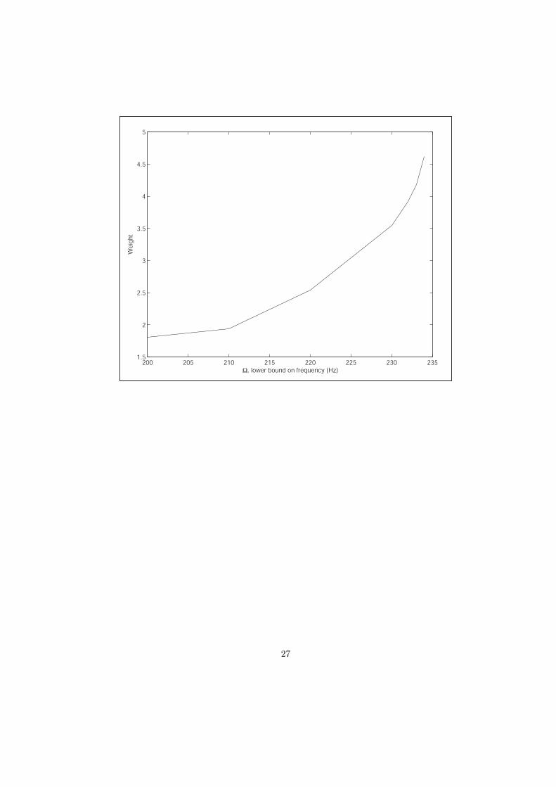
• The problem we consider here is designing a truss such that the lowest frequency¯Ω at which it vibrates is above a given lower bound Ω.

• November 7, 1940, Tacoma Narrows Bridge in Tacoma, Washington

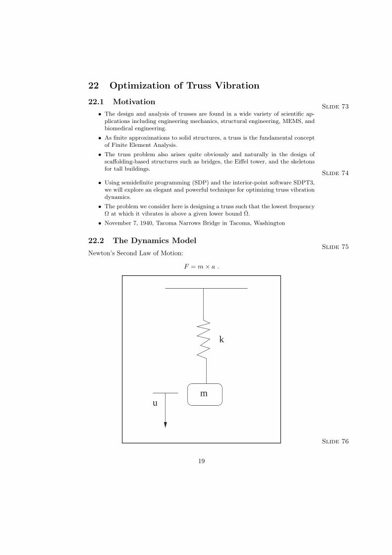
22.2 The Dynamics Model Slide 75

Newton’s Second Law of Motion:

F = m × a .

u m

k

Slide 76

19

√

√

√

√

u m

k

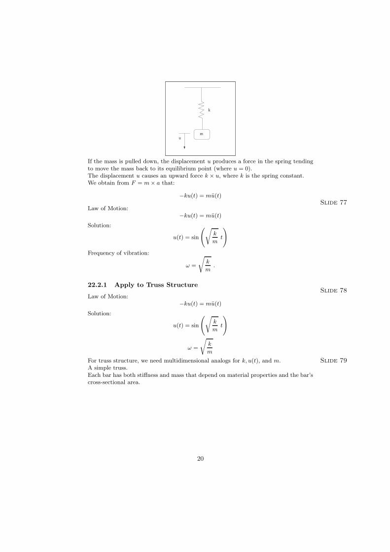
If the mass is pulled down, the displacement u produces a force in the spring tendingto move the mass back to its equilibrium point (where u = 0). The displacement u causes an upward force k × u, where k is the spring constant.We obtain from F = m × a that:

−ku(t) = mu(t) Slide 77

Law of Motion: −ku(t) = mu(t)

Solution: ( ) k

u(t) = sin t m

Frequency of vibration:

k ω = .

m

22.2.1 Apply to Truss Structure Slide 78

Law of Motion: −ku(t) = mu(t)

Solution: ( ) k

u(t) = sin t m

k ω =

m

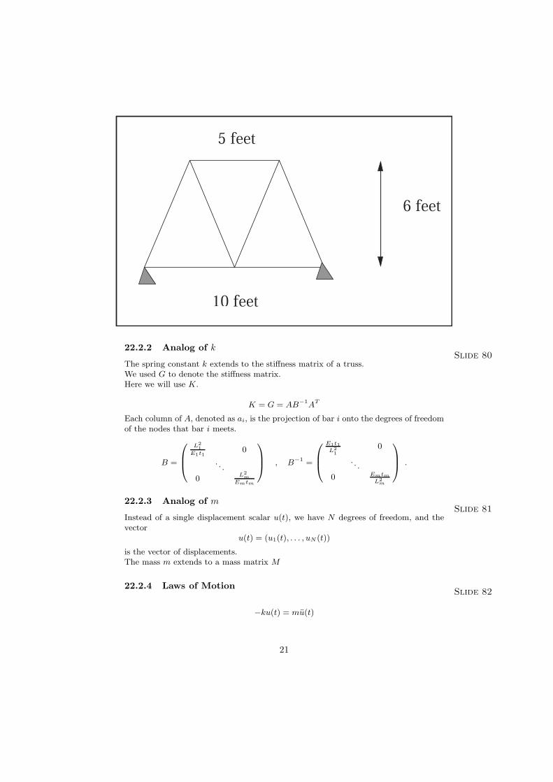
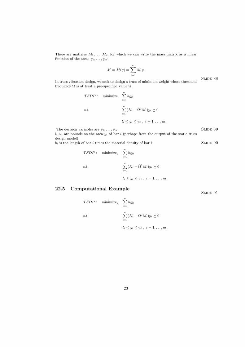
For truss structure, we need multidimensional analogs for k, u(t), and m. Slide 79 A simple truss. Each bar has both stiffness and mass that depend on material properties and the bar’s cross-sectional area.

20

5 feet

6 feet

10 feet

22.2.2 Analog of k Slide 80

The spring constant k extends to the stiffness matrix of a truss.We used G to denote the stiffness matrix.Here we will use K.

TK = G = AB−1A

Each column of A, denoted as ai, is the projection of bar i onto the degrees of freedom of the nodes that bar i meets. 2 E1t1L1 0 L2 0

E1t1 1

B = . . , B−1 = . . . .. 2L

0 m 0 Emtm

Emtm L2 m

22.2.3 Analog of m Slide 81

Instead of a single displacement scalar u(t), we have N degrees of freedom, and the vector

u(t) = (u1(t), . . . , uN (t))

is the vector of displacements.The mass m extends to a mass matrix M

22.2.4 Laws of Motion Slide 82

−ku(t) = mu(t)¨

21

∑ ∑

[

becomes: − Ku(t) = Mu(t)

Both K and M are SPD matrices, and are easily computed once the truss geometry and the nodal constraints are specified. Slide 83

− Ku(t) = Mu(t)

The truss structure vibration involves sine functions with frequencies √

ωi = λi

where λ1, . . . , λN

are the eigenvalues of M−1K

The threshold frequency Ω of the truss is the lowest frequency ωi, i = 1, . . . , N , or equivalently, the square root of the smallest eigenvalue of M−1K. Slide 84

− Ku(t) = Mu(t)

The threshold frequency Ω of the truss is the square root of the smallest eigenvalue of M−1K. Lower bound constraint on the threshold frequency

¯Ω ≥ Ω

Property: ¯ ¯Ω ≥ Ω ⇐⇒ K − Ω2M 0 .

22.3 Truss Vibration Design Slide 85

We wrote the stiffness matrix as a linear function of the volumes ti of the bars i:

m ∑ EiK = ti

L2 (ai)(ai)

T , i

i=1

Li is the length of bar i Ei is the Young’s modulus of bar i ti is the volume of bar i.

22.4 Truss Vibration Design Slide 86

tiHere we use yi to represent the area of bar i (yi = Li

)

m [ m

K = K(y) = Ei

(ai)(ai)T ]

yi = Kiyi Li

i=1 i=1

where

Ki =Ei

(ai)(ai)T ]

, i = 1, . . . , m Li Slide 87

22

∑

∑

∑

∑

∑

∑

∑

There are matrices M1, . . . , Mm for which we can write the mass matrix as a linear function of the areas y1, . . . , ym:

m

M = M(y) = Miyi

i=1

Slide 88 In truss vibration design, we seek to design a truss of minimum weight whose threshold

¯frequency Ω is at least a pre-specified value Ω.

m

TSDP : minimize biyii=1

m ¯s.t. (Ki − Ω2Mi)yi 0

i=1

li ≤ yi ≤ ui , i = 1, . . . , m .

The decision variables are y1, . . . , ym Slide 89 li, ui are bounds on the area yi of bar i (perhaps from the output of the static truss design model) bi is the length of bar i times the material density of bar i Slide 90

m

TSDP : minimizey biyii=1

m ¯s.t. (Ki − Ω2Mi)yi 0

i=1

li ≤ yi ≤ ui , i = 1, . . . , m .

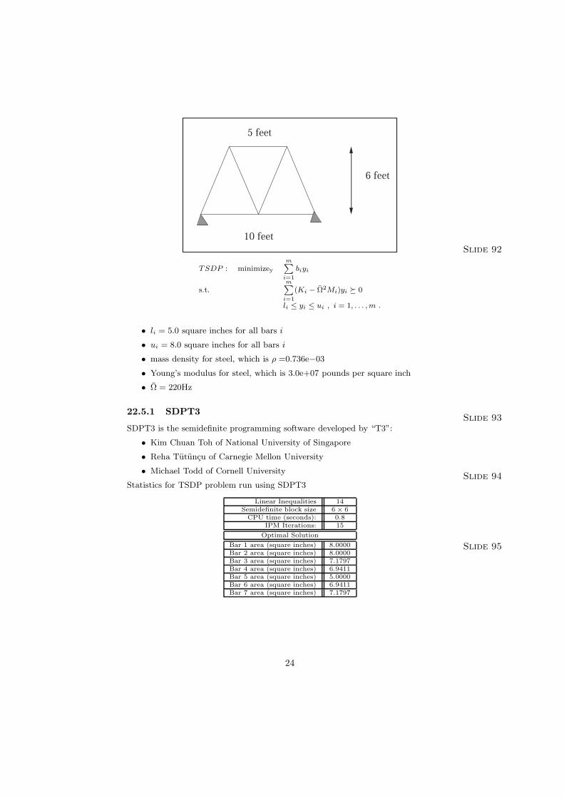
22.5 Computational Example Slide 91

m

TSDP : minimizey biyii=1

m

Ω2Mi)yi 0 i=1

s.t. (Ki − ¯

li ≤ yi ≤ ui , i = 1, . . . , m .

23

∑

∑

5 feet

6 feet

10 feet Slide 92

m

TSDP : minimizey biyii=1m

Ω2Mi)yi 0 i=1

li ≤ yi ≤ ui , i = 1, . . . , m .

s.t. (Ki − ¯

• li = 5.0 square inches for all bars i

• ui = 8.0 square inches for all bars i

• mass density for steel, which is ρ =0.736e−03

• Young’s modulus for steel, which is 3.0e+07 pounds per square inch

¯• Ω = 220Hz

22.5.1 SDPT3 Slide 93

SDPT3 is the semidefinite programming software developed by “T3”:

• Kim Chuan Toh of National University of Singapore

ut¨• Reha T¨ uncu of Carnegie Mellon University

• Michael Todd of Cornell University

Statistics for TSDP problem run using SDPT3

Linear Inequalities Semidefinite block size

CPU time (seconds): IPM Iterations:

Slide 94

14 6 × 6 0.815

Optimal Solution

Bar 1 area (square inches) 8.0000 Bar 2 area (square inches) 8.0000 Bar 3 area (square inches) 7.1797 Bar 4 area (square inches) 6.9411 Bar 5 area (square inches) 5.0000 Bar 6 area (square inches) 6.9411 Bar 7 area (square inches) 7.1797

24

Slide 95

5 feet

6 feet

10 feet

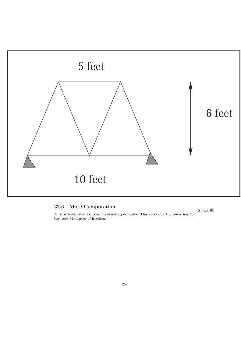
22.6 More Computation Slide 96

A truss tower used for computational experiments. This version of the tower has 40 bars and 32 degrees of freedom.

25

60 40 20 0 20 40 60 0

10

20

30

40

50

60

70

80

90

100 tower

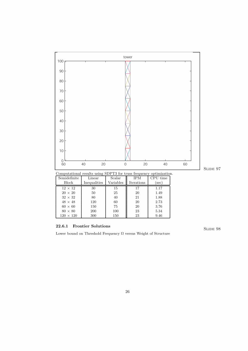
Slide 97 Computational results using SDPT3 for truss frequency optimization.

12 × 12 30 15 17 1.17 20 × 20 50 25 20 1.49 32 × 32 80 40 21 1.88 48 × 48 120 60 20 2.73 60 × 60 150 75 20 3.76 80 × 80 200 100 23 5.34

120 × 120 300 150 23 9.46

Semidefinite Linear Scalar IPM CPU time Block Inequalities Variables Iterations (sec)

22.6.1 Frontier Solutions Slide 98

Lower bound on Threshold Frequency Ω versus Weight of Structure

26

200 205 210 215 220 225 230 235 1.5

2

2.5

3

3.5

4

4.5

5

Ω, lower bound on frequency (Hz)

Wei

ght

27