Embed Size (px)
Citation preview
Introduction to Real Analysis
Mijia Lai
updated on June 11, 2019

2

Contents
1 Preliminary 51.1 Introduction . . . . . . . . . . . . . . . . . . . . . . . . . . . . . . . . . . . . . . . . . 51.2 Cardinality . . . . . . . . . . . . . . . . . . . . . . . . . . . . . . . . . . . . . . . . . 81.3 Euclidean space . . . . . . . . . . . . . . . . . . . . . . . . . . . . . . . . . . . . . . . 9
1.3.1 Topology of the Euclidean space . . . . . . . . . . . . . . . . . . . . . . . . . 91.3.2 Baire Category theorem . . . . . . . . . . . . . . . . . . . . . . . . . . . . . . 91.3.3 Cantor set . . . . . . . . . . . . . . . . . . . . . . . . . . . . . . . . . . . . . . 10
2 Lebesgue measure 132.1 Exterior measure . . . . . . . . . . . . . . . . . . . . . . . . . . . . . . . . . . . . . . 132.2 Measure . . . . . . . . . . . . . . . . . . . . . . . . . . . . . . . . . . . . . . . . . . . 152.3 Borel sets and Measurable sets . . . . . . . . . . . . . . . . . . . . . . . . . . . . . . 182.4 Linear transformation of measurable sets . . . . . . . . . . . . . . . . . . . . . . . . . 202.5 Sets of positive measure . . . . . . . . . . . . . . . . . . . . . . . . . . . . . . . . . . 21
3 Measurable functions 233.1 Measurable functions . . . . . . . . . . . . . . . . . . . . . . . . . . . . . . . . . . . . 233.2 Simple functions . . . . . . . . . . . . . . . . . . . . . . . . . . . . . . . . . . . . . . 243.3 Littlewood’s Three principles . . . . . . . . . . . . . . . . . . . . . . . . . . . . . . . 25
4 Lebesgue’s integration theory 274.1 Integration . . . . . . . . . . . . . . . . . . . . . . . . . . . . . . . . . . . . . . . . . 274.2 Interchanging limits with integrals . . . . . . . . . . . . . . . . . . . . . . . . . . . . 314.3 Lebesgue v.s. Riemann . . . . . . . . . . . . . . . . . . . . . . . . . . . . . . . . . . . 344.4 Fubini’s Theorem . . . . . . . . . . . . . . . . . . . . . . . . . . . . . . . . . . . . . . 36
5 Differentiation 415.1 Monotone functions . . . . . . . . . . . . . . . . . . . . . . . . . . . . . . . . . . . . 415.2 Fundamental theorem of Calculus I . . . . . . . . . . . . . . . . . . . . . . . . . . . . 45
5.2.1 A detour: Bounded variation functions . . . . . . . . . . . . . . . . . . . . . . 465.3 Fundamental theorem of Calculus II . . . . . . . . . . . . . . . . . . . . . . . . . . . 485.4 Lebesgue Differentiation Theorem . . . . . . . . . . . . . . . . . . . . . . . . . . . . 50
6 Function spaces 556.1 LP spaces . . . . . . . . . . . . . . . . . . . . . . . . . . . . . . . . . . . . . . . . . . 55
6.1.1 Normed vector space . . . . . . . . . . . . . . . . . . . . . . . . . . . . . . . . 566.1.2 A detour: Convexity and Jensen’s inequality . . . . . . . . . . . . . . . . . . 576.1.3 Completeness: Banach space . . . . . . . . . . . . . . . . . . . . . . . . . . . 576.1.4 Separability . . . . . . . . . . . . . . . . . . . . . . . . . . . . . . . . . . . . . 58
6.2 Hilbert space: L2 spaces . . . . . . . . . . . . . . . . . . . . . . . . . . . . . . . . . . 59
3

4 CONTENTS
6.2.1 Inner product and Hilbert space . . . . . . . . . . . . . . . . . . . . . . . . . 596.2.2 Orthogonality, Orthonormal basis, Fourier series . . . . . . . . . . . . . . . . 606.2.3 Linear functional, Duality . . . . . . . . . . . . . . . . . . . . . . . . . . . . . 61
Chapter 1
Preliminary
1.1 Introduction
The main subject in this course is the Lebesgue’s integration theory. We have learned in Calculus thata function is Riemannian integrable if and only if the number of discontinuous points is countable.Therefore the Riemannian integral mainly works with almost continuous functions. Even thoughthe great triumph was achieved by the Riemannian integral, it still has a major defect: not workingwell with limit. Indeed, continuous functions are not closed under taking limit, i.e., the limit ofsequence of continuous functions is not necessarily continuous. Moreover, let fn be a sequence ofRiemannian integrable functions on [0, 1], which is convergent to f then
1. f may not be Riemannian integrable;
2. even f is Riemannian integrable,
limn→∞
∫ 1
0
fn(x)dx =
∫ 1
0
f(x)dx
may not hold.
We give a counter-example for item 1 in the above. We can enumerate all rational numbers in[0, 1] as {q1, q2, · · · , ...}, define
fn(x) =
{1, x = q1, q2, · · · , qn;0, else.
It follows that fn converges to the Dirichlet function D(x), which is not Riemannian integrable.
We also provide another interesting counter-example. Let fn(x) = R(x)1n where R(x) is the
Riemann function defined as follows,
R(x) =
{ 1q , x = p
q (p, q) = 1;
0, else.
It follows that the limit of fn is also the Dirichlet function.The basic idea of Riemannian integral is to divide the domain of definition into small intervals
(cubes for higher dimensions). These neighboring intervals (cubes), on the one hand, rely on theunderlining Euclidean geometry, on the other hand, put strong restrictions onto the local behavior ofintegrable functions. (cannot oscillate too much, thus leading to the continuity to some extent) Thegeometric meaning of the Riemannian integral represents the area under the curve, thus Riemann’s
5
6 CHAPTER 1. PRELIMINARY
way of integration, roughly speaking, is to approximate the area by dividing the region into verticalstrips. Lebesgue’s viewpoint is to view the region by horizontal strips. At a first glance, eachhorizontal strip may spread everywhere, however, it turns out to be a sweet surprise. As the localbehavior of the function in consideration is not so critical, and what really matters now is the setof the form {f ≥ c}, which motivates the careful definition of its measure (strictly speaking, in thisbook by measure we mean Lebesgue measure).
This viewpoint dramatically enlarges the range of integrable functions. The corresponding inte-gral theory now boils down to the definition of the measure, and the rest follows almost naturally.Another great advantage of Lebesgue’s integral theory is that it is not restricted only to the inte-gration on Euclidean space. It can equally be transplanted to any abstract measure space, yieldinggreat convenience in subject such as probability theory.
We shall see the above counter-example holds true in the sense of Lebesgue’ integration. Namely,the Dirichlet function is Lebesgue integrable and our hope that limn→∞
∫[0,1]
fn(x)dx =∫
[0,1]D(x)dx
becomes true.Vocabulary-wise, in this course we shall provide the following generalization:
length, area, volume, ... =⇒ measure
continuous functions =⇒ measurable functions
Riemannian integral =⇒ Lebesgue integral
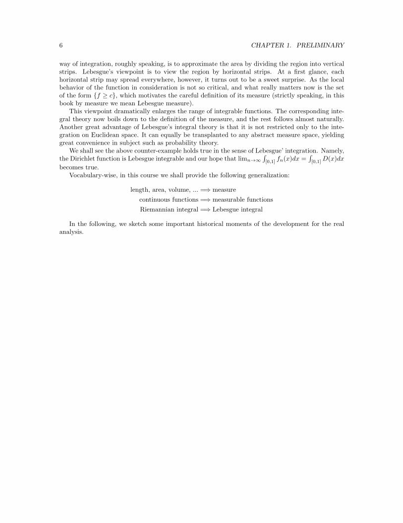
In the following, we sketch some important historical moments of the development for the realanalysis.
2
Some Historical developments of real analysis
Weierstrass’s nowhere
differentiable function
1872
Introduction of BV
functions by Jordan and
later connection with
rectifiability
Cantor set
Space filling curve by
Peano
Construction of
non-measurable sets by
Vitali
Borel’s measurable sets
Lebesgue’s theory of
measure and integration
1881
1883
1890
1898
1902
1905

8 CHAPTER 1. PRELIMINARY
1.2 Cardinality
In following sections, we establish some foundations on the set theory and the topology and geometryof the Euclidean space. We assume the reader is familiar with basic notions of sets, operationsbetween sets, etc. In this section, we address the following question: how to compare two sets withinfinite elements? This requires the concept of the cardinality of a set.
For two sets with finite number of elements, it is clear which set contains more elements. For twosets with infinite elements, which contains ’more’ elements relies on the mappings between them.
A map f : A → B is an assignment to each element of A a unique element in B. f is calledinjective, if f(x) 6= f(y), for x 6= y. f is called surjective if ∀z ∈ B, there exists x ∈ A such thatf(x) = z. A map f : A→ B is called a bijection if f is both injective and surjective. Clearly, a mapf : A→ B has a well-defined inverse, if and only if f is a bijection.
We say two sets A and B are of same cardinality if there exists a bijection f : A → B. It isdenoted by A ∼ B. Sometimes, we shall refer to the cardinal number of a set A, denoted by ¯A.
The cardinal number of natural numbers N is denoted by ℵ0. (Countable)
Example 1. Each infinite set contains a countable subset.
Example 2. Countable union of countable sets is countable.
Proof. Array this union as an infinite square, and enumerate in a zigzag way.
Example 3. All rational numbers Q is countable.
Example 4. Finite cartesian product of countable sets is countable.
Proof. Visualize this union as an infinite k dimensional cube, and enumerate in a zigzag way.
Example 5. The set of all real numbers R is not countable.
Proof. We prove (0, 1] is not countable. We accept each real number in (0, 1] has a decimal repre-sentation, which is unique if we don’t allow the appearance of all zeros after some position. That iswe write 0.25 as 0.249999999..., 1 as 0.99999...., etc.
Now suppose (0, 1] is countable, then we have an enumeration for all numbers in (0, 1], say0.a11a12a13...., 0.a21a22a23..., ... We can choose bii ∈ {0, 1, 2, ..., 9} \ aii, for each i. Let y =0.b11b22b33..., a moment of thought shows that y is indeed not in the enumeration list. A contradic-tion.
The cardinality of R is called ℵ1. The decimal representation shows that countable product offinite sets has cardinal number ℵ1.
Example 6. R, (0, 1], [0, 1], Rn all have same cardinal number ℵ1.
Theorem 1.1. There does not exist maximal cardinal number.
Proof. Given any set A, consider its power set 2A, namely the set of all subsets of A. We canshow they have different cardinality. Otherwise, there exists a bijection f : A → 2A, where f(a)corresponds to a subset of A. Define a subset of A as follows:
B = {x|x /∈ f(x)}.
Now an amusing question confronts us: is B = f(x) for some x ∈ A?This proof is reminiscent of the barber paradox, which was raised by Bertrand Russell as follows:
a barber in a town claims to be the ”one who shaves all those, and those only, who do not shavethemselves.” The question is, does the barber shave himself?
1.3. EUCLIDEAN SPACE 9
Remark 1.2 (Continuum hypothesis). Cantor in 1878 raised the following hypothesis concerning thesize of infinite sets:
There is no set whose cardinality is strictly between that of the integers and the real numbers.
Establishing its truth or falsehood is the first of Hilbert’s 23 problems presented in 1900. The readeris referred to https://en.wikipedia.org/wiki/Continuum hypothesis for a thorough introduction.
1.3 Euclidean space
1.3.1 Topology of the Euclidean space
We use Rn for n-dimensional Euclidean space. For x = (x1, · · · , xn and y = (y1, · · · , yn), the innerproduct is defined as
x · y = x1y1 + x2y2 + · · ·+ xnyn.
Norm is defined as
|x| =√x2
1 + · · ·+ x2n.
Open ball centered at x of radius r is denoted by B(x, r), i.e.,
B(x, r) = {y||y − x| < r}.
Given A ⊂ Rn, x is called an interior point of A if there exists r > 0 such that B(x, r) ⊂ A. Ais called an open set, if every point of A is an interior point.
A is bounded if there exists R > 0, such that A ⊂ B(0, R). A set is called compact if it is bothbounded and closed. A nice property of being a compact set is that any open cover has a finitesubcover.
x is called an accumulation point of A, if (B(x, r) \ {x}) ∩ A 6= ∅, for all r > 0. The union ofA with its accumulation points is called the closure of A, denoted by A. A subset B ⊂ A is calleddense in A, if B = A. A is called nowhere dense if there exists no interior point of A.
1.3.2 Baire Category theorem
Given a set X, a map d : X ×X → R+ satisfying
1. Symmetry d(x, y) = d(y, x);
2. Positivity d(x, y) ≥ 0 and = holds if and only if x = y;
3. Triangle inequality d(x, y) + d(y, z) ≥ d(x, z);
is called a metric on X. (X, d) is then called a metric space.Using metric, one can define the notion of convergence. limn→∞ xn = x if and only if limn→∞ d(xn, x) =
0. {xn} is called a Cauchy sequence, if
∀ε > 0, there exists N , such that d(xn, xm) ≤ ε,∀n,m > N.
A metric space is called complete if any Cauchy sequence is convergent in the space.The concepts of open balls, open sets, closed sets, interior points, closure, etc, all generalize to
the metric space.
Theorem 1.3 (Baire Category Theorem). A non-empty complete metric space is not a countableunion of nowhere dense sets.

10 CHAPTER 1. PRELIMINARY
Proof. Suppose not. Then assume X =⋃∞n=1Dn, where each Dn is a nowhere dense set. Clearly
X \ D1 is not empty, therefore there exists an interior point x1 and ε1 > 0 such that B(x1, ε1) ⊂X \D1. Similarly D2
c ∩B(x1, ε) is a nonempty open set, we can choose x2, ε2 such that B(x2, ε2) ⊂D2
c ∩B(x1, ε). Inductively, we get a sequence of nested balls B(xn, εn) ⊂ B(xn−1, εn−1), moreoverwe can easily arrange that limn→∞ εn = 0. Thus {xn} is a Cauchy sequences and it converges to,say x. Since X =
⋃∞n=1Dn, thus x ∈ Dk for some k. However due to the construction x ∈ B(xk, εk),
which contradicts to that B(xk, εk) ∩Dk = ∅.
Using the Baire category theorem, we get another proof that [0, 1] is uncountable.Countable intersection of open sets is called a Gδ set, countable union of closed sets is called an
Fσ set. We give a more interesting application of Baire’s category theorem.
Proposition 1.4. There does not exist a function f : R→ R which is continuous only at all rationalnumbers.
We need a lemma first.
Lemma 1.5. The points of continuity of f is a Gδ set.
Proof. Recall that f is continuous at x if and only if the oscillation ωf (x) = 0. Therefore the set ofpoints of continuity of f is
∞⋂n=1
{x|ωf (x) <1
n}.
It is easy to show that {x|ωf (x) < 1n} is open.
Proof of the Proposition. Using the above lemma, it is suffice to show that Q is not a Gδ set. Supposenot, then assume
Q =
∞⋂n=1
Gn,
where each Gn is open set. We write Q as Q = {q1, q2, · · · }, then
R =
∞⋃n=1
Gcn
∞⋃i=1
{qi}.
Gcn is closed, suppose it contains an interior point, then there exists an open interval (x, y) ⊂ Gcn.Therefore
(x, y)c ⊃ Gn ⊃ Q.
The only possible case is x = y. Hence Gcn is nowhere dense.The above expression writes R as a union of countable nowhere dense sets. This contradicts to
the Baire category theorem.
1.3.3 Cantor set
Let C0 = [0, 1] the unit closed interval. C1 = [0, 13 ] ∪ [ 2
3 , 1], the removal of the middle 13 open
interval from C0. Cn is obtained inductively by removing the middle one third open intervals ofeach connected components of Cn−1. For example, C2 = [0, 1
9 ] ∪ [ 29 ,
13 ] ∪ [ 2
3 ,79 ] ∪ [ 8
9 , 1].
C :=
∞⋂n=0
Cn
is the Cantor set.The following proposition lists several properties of the Cantor set.

1.3. EUCLIDEAN SPACE 11
Figure 1.1: Cantor set
Proposition 1.6. The Cantor set C defined as above is non-empty and satisfies the followingproperties:
• C is closed.
• C does not contain any interior point, hence it is nowhere dense.
• C is uncountable, and its cardinal number is ℵ1.
Proof. C is not empty. A moment of thought shows that the end points of those middle thirdintervals all remain in C. Since each Cn is closed, the intersection of countable closed sets is stillclosed.
Suppose x ∈ C is an interior point, then there exists δ > 0, such that (x− δ, x+ δ) ⊂ C. TakingN large enough such that 1
3N < 2δ, it follows (x − δ, x + δ) is not contained in CN , as the lengthof each connected component of CN is 1
3N . This shows that C does not have any interior points.Together with closeness of C, it follows that C is nowhere dense.
Using the decimal representation of base 3 for all real numbers in [0, 1], i.e, x =∑∞i=1
ai3i , where
ai ∈ {0, 1, 2}. Again to ensure the uniqueness, we don’t allow the situation that ai = 0 ∀i ≥ Nfor some N , unless x = 0 which corresponds to ai = 0 for all i. The removal of the middle thirdintervals prevents the appearance of 1 in this decimal representation. Therefore C ∼ {0, 2}N whichhas the cardinal number ℵ1.

12 CHAPTER 1. PRELIMINARY

Chapter 2
Lebesgue measure
In this chapter, we shall generalize ’length, area, volume, ...’ of regular regions to the measure ofarbitrary sets. There are two steps involved. The idea of the first step is to approximate a general setby familiar regular sets: open cubes. However, this approximation is more plausible from exterior ofa set, which leads to the definition of the exterior measure. The second step is the discovery that toencompass the property of the disjoint additivity, one has to disregard some sets of highly irregular(non-measurable sets). Therefore a satisfactory measure theory does not include all subsets of Rn.
2.1 Exterior measure
As said above, measure is a generalization of ’length, area, volume, ...’ . So the very first agreementis that the measure of the n-dimensional open cube C = (a1, b1) × · · · (an, bn) is its volume (b1 −a1)× · · · (bn − an), and measure of regular regions are their volume. Moreover, geometric intuitionechoes that any such generalization should inherit nice properties of volume, such as
• monotone: if A ⊂ B, then A’s measure is not greater than B’s measure;
• disjoint additivity: ∪ni=1Ai’s measure is the sum of Ai’ measure if Ai are disjoint;
• translation invariant;
• Scaling property.
We use the covering of cubes to define the measure for a general set, and we shall allow countablemany cubes for the covering.
Definition 2.1. Given E ⊂ Rn, the exterior measure of E is defined as
m∗(E) := infE⊂∪∞k=1Ik
∞∑k=1
|Ik|,
where {Ik}∞k=1 is a sequence of countable open cubes that cover E and |Ik| is the volume of Ik.
The reason we call it exterior measure rather than measure will be clear momentarily. Before thatwe shall get used to this definition by exploring several simple yet important facts and properties ofthe exterior measure.
Example 7. Let A be a set consists of countable many points, then m∗(A) = 0.
13

14 CHAPTER 2. LEBESGUE MEASURE
Proof. This proof is a common trick in real analysis, which relies on
∞∑n=1
ε
2n= ε.
Example 8. m∗(C) = 0, where C is the Cantor set.
Remark 2.2. The definition builds on the volume of n-dimensional cubes. Therefore it can’t distin-guish sets of ’lower dimension’. For example, a line segment in R2 has exterior measure (area) zero,but it certainly has length. The more intrinsic way to encode the dimension information of sets isthe notion called Hausdorff measure.
The next theorem shows that the exterior measure has all the nice properties we could expect.
Theorem 2.3. The exterior measure satisfies the following
• nonnegativity: m∗(E) ≥ 0;
• monotone: if A ⊂ B, then m∗(A) ≤ m∗(B);
• sub-additivity: m∗(∪∞k=1Ak) ≤∑∞k=1m
∗(Ak);
• translation invariant: m∗(E + {x0}) = m∗(E);
• scaling: m∗(λE) = λnm∗(E); ∀λ > 0.
Proof. We only prove the sub-additivity. The rests follow more or less directly from definition andthus are left to the reader. ∀ε > 0, there exists a covering of open cubes {Ik,i} for each Ak, suchthat
m∗(Ak) ≤∞∑i=1
|Ik,i| ≤ m∗(Ak) +ε
2i.
Clearly ∪∞i,k=1Ii,k is a countable union of open cubes that covers ∪∞k=1Ak, thus
m∗(∪∞k=1Ak) ≤∞∑k=1
∞∑i=1
|Ik,i| ≤∞∑k=1
m∗(Ak) + ε.
Since ε is arbitrary, we get the desired sub-additivity.
There is still one unsatisfied issue: the exterior measure only has subadditivity, and is lack ofadditivity for disjoint sets. That is
m∗(∪∞k=1Ak) =
∞∑k=1
m∗(Ak)
whenever Ak are disjoint. Here is an example.
Example 9. [A non-measurable set] We shall construct a set N ⊂ [0, 1]. First, we define an equivalentrelation, say x ∼ y if x− y ∈ Q. Under this equivalent relation, [0, 1] can be written as the disjointunion of different equivalent classes:
[0, 1] =⋃α∈Λ
Eα.
We pick a representative rα ∈ Eα in each equivalent class and set N := {rα}α∈Λ.
2.2. MEASURE 15
Denote all rational numbers in [−1, 1] as {q1, q2, · · · , }. We claim Nk := N + qk are disjoint.Suppose Nk ∩ Nl 6= ∅, then there exists x, y ∈ N , such that x + qk = y + ql, which means x ∼ y.This contradicts the only one pick from each equivalent class.
If Nk satisfied the disjoint additivity, we would have
m∗(
∞⋃k=1
Nk) =
∞∑k=1
m∗(Nk).
Clearly,
[0, 1] ⊂∞⋃k=1
Nk ⊂ [−1, 2],
and thus
1 ≤∞∑k=1
m∗(Nk) ≤ 3. (2.1)
In view of the translation invariant, m∗(Nk) = m∗(N),∀k. No value for m∗(N) would justify (2.1).
Remark 2.4. We shall point out, the definition of N , namely the pick of one element from eachequivalent class requires the Axiom of choice. Formally, it states that for every indexed family(Si)i∈I of nonempty sets there exists an indexed family (xi)i∈I of elements such that xi ∈ Sifor every i ∈ I. The reader is referred to https://en.wikipedia.org/wiki/Axiom of choice for moredetails.
2.2 Measure
The example 9 shows in general we do not have disjoint additivity of exterior measure for all subsetsof Rn. A remedy is to restrict our attention to those sets, for which the disjoint additivity hold.
Caratheodory made the following convenient criterion for the sets we shall be concerned with.
Definition 2.5. Let A ⊂ Rn, A is called a measurable set if
m∗(T ) = m∗(T ∩A) +m∗(T ∩Ac), ∀T ⊂ Rn. (2.2)
A useful observation is that to verify (2.2), one just needs to showm∗(T ) ≥ m∗(T∩A)+m∗(T∩Ac)Since m∗(T ) ≤ m∗(T ∩A) +m∗(T ∩Ac) always holds by the sub-additivity.
Suppose m∗(A) = 0, then m∗(T ∩ A) = 0 and m∗(T ∩ Ac) ≤ m∗(T ), we infer that all sets withzero exterior measure are measurable.
The collection of all measurable sets is denoted by M. We prove the following
Theorem 2.6. 1. ∅ ∈ M;
2. if A ∈M, then Ac ∈M;
3. if Ak ∈M for k = 1, 2, · · · , then ∪∞k=1Ak ∈M, moreover
m∗(∪∞k=1Ak) =
∞∑k=1
m∗(Ak)
whenever Ak are disjoint.

16 CHAPTER 2. LEBESGUE MEASURE
Proof. Notice (2.2) is symmetric about A and Ac, 2 of the theorem immediately follows. To show 3,we first show if A1, A2 ∈M, then A1 ∪A2 ∈M. Using A1, A2 are measurable, we have for any T ,
m∗(T ) = m∗(T ∩A1) +m∗(T ∩Ac1)
= m∗(T ∩A1 ∩A2) +m∗(T ∩A1 ∩Ac2) +m∗(T ∩Ac1 ∩A2) +m∗(T ∩Ac1 ∩Ac2).
Notice T ∩ (A1 ∪A2) = (T ∩A1 ∩A2)∪ (T ∩A1 ∩Ac2)∪ (T ∩Ac1 ∩A2), by sub-additivity, we have
m∗(T ∩ (A1 ∪A2)) ≤ m∗(T ∩A1 ∩A2) +m∗(T ∩A1 ∩Ac2) +m∗(T ∩Ac1 ∩A2),
and thus
m∗(T ) ≥ m∗(T ∩ (A1 ∪A2)) +m∗(T ∩Ac1 ∩Ac2) = m∗(T ∩ (A1 ∪A2)) +m∗(T ∩ (A1 ∪A2)c).
This implies that A1 ∪A2 ∈M.Moreover suppose A1 ∩A2 = ∅, then setting T = A1 ∪A2 in m∗(T ) = m∗(T ∩A1) +m∗(T ∩Ac1),
we get the additivity for two disjoint sets:
m∗(A1 ∪A2) = m∗(A1) +m∗(A2). (2.3)
Setting T of the form T ∩ (A1 ∪A2) we also have
m∗(T ∩ (A1 ∪A2)) = m∗(T ∩A1) +m∗(T ∩A2). (2.4)
Iterate this process finite many times together with the property 2, we infer that if A1, · · ·An ∈M, then any union or intersection among them is still measurable, and finite disjoint additivityholds, i.e.,
m∗(∪ni=1Ai) =
n∑i=1
m∗(Ai),
and
m∗(T ∩ (∪ni=1Ai)) =
n∑i=1
m∗(T ∩Ai),
whenever Ai are all disjoint.For countable union, first suppose A1, · · · , An, · · · ∈ M are all disjoint. Let S := ∪∞n=1An and
Sk = ∪kn=1An. Using Sk ∈M, we have for any T that
m∗(T ) = m∗(T ∩ Sk) +m∗(T ∩ Skc)
=
k∑n=1
m∗(T ∩An) +m∗(T ∩ Skc) ≥
k∑n=1
m∗(T ∩An) +m∗(T ∩ Sc).
Above inequality holds for all k, letting k →∞ we obtain
m∗(T ) ≥∞∑n=1
m∗(T ∩An) +m∗(T ∩ Sc) ≥ m∗(T ∩ S) +m∗(T ∩ Sc).
Hence S ∈M.Using T ∩ S in the above inequality, we get
m∗(T ∩ S) ≥∞∑n=1
m∗(T ∩An).
2.2. MEASURE 17
On the other hand, m∗(T ∩ S) ≤∑∞n=1m
∗(T ∩An) always holds by sub-additivity. Therefore
m∗(T ∩ S) =
∞∑n=1
m∗(T ∩An),
by taking T = Rn, we get the disjoint additivity.
Finally, if {An} ∈ M are not necessarily disjoint from each other, then we make the followingchange:
B1 = A1, Bk = (∪ki=1Ai) \ ((∪k−1i=1 Ai)) ∀k ≥ 2.
It follows {Bk} are disjoint and ∪∞n=1An = ∪∞k=1Bk ∈M.
From now on we shall write simply m(A) for the exterior measure of a measurable set A. Ourtask of defining the measure for suitable subsets of Rn is now completed.
We conclude this section with two useful facts about interchanging measure with limit operation.
Proposition 2.7. Let An ⊂ An+1 be a sequence of increasing measurable sets, set A = ∪nAn, then
m(A) = limn→∞
m(An).
Proof. If m(An) =∞ for some n, then the desired equality holds. Therefore we assume m(An) <∞for all n. Set B1 = A1, B2 = A2 \ A1, Bn = An \ An−1, then Bn are all disjoint. Using countabledisjoint additivity, we get
m(∪nBn) =
∞∑k=1
m(Bk).
We obtain the desired equality as ∪nBn = ∪nAn and m(An) =∑nk=1m(Bk).
For decreasing sequence, we have
Proposition 2.8. Let An ⊃ An+1 be a sequence of decreasing measurable sets, set A = ∩nAn,assume m(A1) <∞ then
m(A) = limn→∞
m(An). (2.5)
Proof. We view A1 as the ambient set and take complement with respect to A1. We then have
∅ ⊂ Ac2 ⊂ · · · ⊂ Acn · · · ,
Applying Proposition 2.7, we have
m(∪nAcn) = limn→∞
m(Acn). (2.6)
Since
m(Acn) +m(An) = m(A1) and m(∪nAcn) +m(A) = m(A1),
plugging back to (2.6), we get (2.5).
Remark 2.9. The assumption m(A1) <∞ is necessary. For example, let An = (n,∞), then ∩nAn =∅ and (2.5) fails.

18 CHAPTER 2. LEBESGUE MEASURE
2.3 Borel sets and Measurable sets
In this section, we explore some relation between measurable sets and open, closed sets. Thefirst question we should answer is whether open cubes are measurable? The answer is definitelyaffirmative:
Theorem 2.10. If G is an open set, then G is measurable.
We need two lemmas. First recall two definitions. The distance between a point and a set isdefined as
d(x,A) = infy∈A
d(x, y),
and the distance between two sets is defined as
d(A1, A2) = infx∈A1,y∈A2
d(x, y).
Lemma 2.11. Let A1, A2 be two sets with d(A1, A2) > 0, then
m∗(A1 ∪A2) = m∗(A1) +m∗(A2).
Proof. Observe first that in the definition of the exterior measure, we could require the side lengthesof all open cubes are ≤ δ for a fixed δ > 0. To prove the lemma, we just need to show m∗(A1∪A2) ≥m∗(A1) +m∗(A2). Suppose d(A1, A2) = 2δ > 0, then for any ε > 0, there exit countable open cubes{Di} of side lengthes ≤ δ covering A1 ∪A2 such that
m∗(A1 ∪A2) + ε ≥∞∑i=1
|Di|.
We can divide {Di} into two groups {D(1)j } and {D(2)
j } such that
∪∞j=1D(1)j ⊃ A1 and ∪∞j=1 D
(2)j ⊃ A2.
Since d(A1, A2) = 2δ > 0, all side lengthes ≤ δ, it follows that D(1)k ∩D
(2)l = ∅, ∀k, l. Hence
m∗(A1 ∪A2) + ε ≥∞∑i=1
|Di| =∞∑j=1
|D(1)j |+
∞∑j=1
|D(2)j | ≥ m
∗(A1) +m∗(A2).
Since ε is arbitrary, we get the desired inequality.
Lemma 2.12. [Caratheodory] Suppose G 6= Rn is an open set, E ⊂ G, let
Ek = {x ∈ E : d(x,Gc) ≥ 1
k}, k = 1, 2, · · · ,
then limk→∞
m∗(Ek) = m∗(E).
Proof. Clearly, Ek ⊂ Ek+1 ⊂ E and ∪∞k=1Ek = E, it follows that m∗(Ek) is monotone increasingand limk→∞m∗(Ek) ≤ m∗(E).
It remains to show that m∗(E) ≤ limk→∞m∗(Ek). It suffices to assume limk→∞m∗(Ek) < ∞.Let Ak = Ek \ Ek−1, then d(Ak, Ak+2) > 0. Note
m∗(E2k) ≥ m∗(∪ki=1A2i) =
k∑i=1
m∗(A2i).
2.3. BOREL SETS AND MEASURABLE SETS 19
The equality is due to Lemma 2.11. In view of the assumption limk→∞m∗(Ek) <∞,∑∞i=1m
∗(A2i)
is convergent. Similarly,∑ki=1m
∗(A2i−1) is also convergent.Since E = E2k ∪ (∪j>kA2j) ∪ (∪j>kA2j−1), by sub-additivity, we have
m∗(E) ≤ m∗(E2k) +m∗(∪j>kA2j) +m∗(∪j>kA2j−1)
≤ m∗(E2k) +∑j>k
m∗(A2j) +∑j>k
m∗(A2j−1).
Letting k →∞, we obtain that m∗(E) ≤ limk→∞m∗(E2k). This completes the proof.
Proof of Theorem 2.10. We just need to show
m∗(T ) ≥ m∗(T ∩G) +m∗(T ∩Gc), ∀T ⊂ Rn.
By Lemma 2.12, there exist sets Tk ⊂ T ∩G, such that
limk→∞
m∗(Tk) = m∗(T ∩G).
Sincem∗(T ) ≥ m∗(Tk) +m∗(T ∩Gc),
letting k →∞, we get the desired inequality.
Definition 2.13. A collection T of subsets of X satisfying
• ∅ ∈ T ;
• if A ∈ T , then Ac ∈ T ;
• if Ak ∈ T for k = 1, 2, · · · , then ∪∞k=1Ak ∈ T ;
is called a σ-algebra.
Given a collection Γ of subsets of X, the minimal σ-algebra containing Γ is called the σ-algebragenerated by Γ. In Rn, the σ-algebra generated by all open sets is called the Borel algebra, denotedby B. Its element is called a Borel set. Therefore, all closed sets, Gδ sets, Fσ sets, and their countableunions, etc, are all Borel sets.
Then a direct consequence of Theorem 2.10 is
Corollary 2.14. All Borel sets are measurable.
Finally we show up to a set of measure zero, a measurable set is either a Gδ or an Fσ set.
Proposition 2.15. Let A be a measurable set, then ∀ε > 0,
• there exists an open set G ⊃ A, such that m(G \A) < ε;
• there exists a closed set F ⊂ A, such that m(A \ F ) > ε.
Proof. First assume m(A) <∞. Then ∀ε > 0, there exists countable open cubes Di covering A suchthat
∞∑i=1
|Di| < m(A) + ε.
Let G = ∪∞i=1Di which is an open set containing A. Since A is measurable, we have
m(G \A) = m(G)−m(A) ≤∞∑i=1
|Di| −m(A) < ε.

20 CHAPTER 2. LEBESGUE MEASURE
For m(A) = ∞, we let An := A ∩ B(0, n). For fixed ε > 0 and n, there exists an open setGn ⊃ An, such that
m(Gn \An) <ε
2n.
Let G = ∪nGn, it follows that G ⊃ A is an open set and
m(G \A) ≤∞∑n=1
m(Gn \An) ≤ ε.
The second statement can be obtained dually by the De Morgan’s law.
Remark 2.16. Instead of the Caratheodory criterion, one can use the first statement of the Propo-sition to define measurable set. The reader is referred to Stein’s book for this treatment.
Proposition 2.17. Let A be a measurable set, then
• there exists a Gδ set G ⊃ A, such that m(G \A) = 0;
• there exists an Fσ set F ⊂ A, such that m(A \ F ) = 0.
Proof. By Proposition 2.15, for ε = 1n , there exists an open set Gn ⊃ A such that
m(Gn \A) <1
n.
Let G = ∩∞n=1Gn, it follows that G ⊃ A and
m(G \A) ≤ m(Gn \A) <1
n, ∀n.
Hence m(G \A) = 0. The second statement follows similarly.
2.4 Linear transformation of measurable sets
In this section, we briefly discuss how to obtain classical area formula for triangle and disk in ameasure theoretical way. What we use are the properties of measure and the transformation law ofmeasure of a set under linear transformations. The latter can be viewed as the change of variableformula in multi-variable Calculus.
Theorem 2.18. Let T : Rn → Rn be a non-singular linear transformation, then for any measurableset A,
m(T (A)) = |det(T )|m(A). (2.7)
Proof. The proof is divided into two steps.Step 1: reduction of A to unit cubeFrom Proposition 2.17, a general measurable set A differs from a Gδ set AG by a set of measurezero, and any open set is countable union of open cubes. Therefore it suffices to verify (2.7) for unitcube D0.
Step 2: decomposition of a linear transformation into following three simple transformations:
1. T (xi) = xj , T (xj) = xi, T (xk) = xk for k 6= i, j;
2. T (x1) = λx1, T (xi) = xi for i ≥ 2 and λ 6= 0;
2.5. SETS OF POSITIVE MEASURE 21
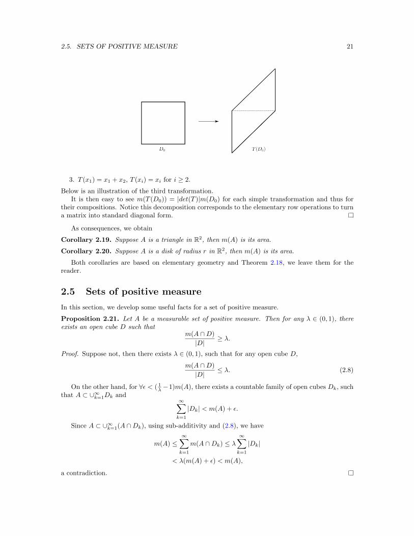
3. T (x1) = x1 + x2, T (xi) = xi for i ≥ 2.
Below is an illustration of the third transformation.It is then easy to see m(T (D0)) = |det(T )|m(D0) for each simple transformation and thus for
their compositions. Notice this decomposition corresponds to the elementary row operations to turna matrix into standard diagonal form.
As consequences, we obtain
Corollary 2.19. Suppose A is a triangle in R2, then m(A) is its area.
Corollary 2.20. Suppose A is a disk of radius r in R2, then m(A) is its area.
Both corollaries are based on elementary geometry and Theorem 2.18, we leave them for thereader.
2.5 Sets of positive measure
In this section, we develop some useful facts for a set of positive measure.
Proposition 2.21. Let A be a measurable set of positive measure. Then for any λ ∈ (0, 1), thereexists an open cube D such that
m(A ∩D)
|D|≥ λ.
Proof. Suppose not, then there exists λ ∈ (0, 1), such that for any open cube D,
m(A ∩D)
|D|≤ λ. (2.8)
On the other hand, for ∀ε < ( 1λ −1)m(A), there exists a countable family of open cubes Dk, such
that A ⊂ ∪∞k=1Dk and∞∑k=1
|Dk| < m(A) + ε.
Since A ⊂ ∪∞k=1(A ∩Dk), using sub-additivity and (2.8), we have
m(A) ≤∞∑k=1
m(A ∩Dk) ≤ λ∞∑k=1
|Dk|
< λ(m(A) + ε) < m(A),
a contradiction.
22 CHAPTER 2. LEBESGUE MEASURE
Theorem 2.22 (Steinhaus). Let A be a measurable set of positive measure. Then there exists δ > 0,such that
A−A ⊃ B(0, δ),
where A−A := {x− y|x, y ∈ A}.
Another way of saying A−A ⊃ B(0, δ) is that translating A by a vector u ∈ B(0, δ) will intersectA, i.e., a small movement of a set of positive measure will always overlap with itself. You can imaginea set of positive measure as your favorite Chinese papercut.
Figure 2.1: Chinese papercut
Proof. Using Proposition 2.21, for a fixed λ ∈ (0, 1), we could find an open cube D such that
m(A ∩D)
|D|> λ.
For simplicity, let AD = A ∩ D, we shall show the theorem holds for AD, then it holds for A aswell. Suppose AD − AD does not contain an open ball centered at 0, then for any δ, there existsv ∈ Rn, |v| < δ such that AD ∩ AD + {v} = ∅. For simplicity, let us denote AD + {v} by A′D, andD + {v} = D′.
m(D ∪D′) ≥ m(AD ∪A′D) = m(AD) +m(A′D) > 2λm(D).
We get a contradiction if δ is sufficiently small, as m(D ∪D′) is then very close to m(D).

Chapter 3
Measurable functions
3.1 Measurable functions
We consider an extended real value function f : Rn → {±∞} ∪ R. f is called finite-valued if−∞ < f(x) < ∞, ∀x. Let f be a function defined on a measurable subset E of Rn, f is called ameasurable function, if ∀a ∈ R, the set
f−1((a,∞]) := {x ∈ E|f(x) > a}
is measurable.Using some set operations, we shall see this definition has many equivalent versions;
Proposition 3.1. Suppose f is a measurable function, then the following sets are also measurable.
• {x : f(x) ≤ t}(t ∈ R);
• {x : f(x) ≥ t}(t ∈ R);
• {x : f(x) < t}(t ∈ R);
• {x : f(x) = t}(t ∈ R);
• {x : f(x) < +∞};
• {x : f(x) = +∞};
• {x : f(x) > −∞};
• {x : f(x) = −∞}.
Using definition, it is easy to verify the following:
Proposition 3.2. Let f, g be two measurable functions defined on E, then
f ± g; cf, ∀c ∈ R; f · g
are all measurable functions.
Proof. We verify according to definitions. Let Q = {qj}∞j=1, we claim
{f + g > t} = ∪∞j=1({f > qj} ∩ {g > t− qj}),
23

24 CHAPTER 3. MEASURABLE FUNCTIONS
then it follows that {f + g > t} is measurable. To show the claim, it is clear the right hand sideis contained in the left hand side. For the reverse direction, take x ∈ {f + g > t} and supposef(x) + g(x) = t+ δ. Then there exists a rational q such that
q < f(x) < q +δ
2,
from which we get g(x) > t− q. Thus x ∈ {f > q} ∩ {g > t− q} for this particular q.To show f · g is measurable, we first show f2 is measurable, then using
f · g =1
2{(f + g)2 − f2 − g2}.
For f2, clearly we have
{f2 > t} =
{{f >
√t} ∪ {f < −
√t}, t ≥ 0,
Rn, t < 0.
Then the conclusion easily follows.
Measurable functions are very friendly with limit operation.
Proposition 3.3. Let {fk(x)} be a sequence of measurable functions on E, then
• supk{fk(x)};
• infk{fk(x)};
• lim supk fk(x);
• lim infk fk(x);
are all measurable.
A direct consequence is that if the limit of a sequence of measurable function is measurable.We shall in the following often deal with statements, which hold true for all x but a set of measure
zero. In such case, we shall say a statement P (x) holds true almost everywhere, and it is abbreviatedas P (x), a.e. x. For example,
limn→∞
fn(x) = f(x), a.e.x ∈ E
means there exists a set Z ⊂ E of measure 0, such that fn(x) converges to f(x) for x ∈ E \ Z.The next proposition shows a general viewpoint in dealing with measurable functions.
Proposition 3.4. Let f(x) = g(x), a.e., suppose f(x) is a measurable function, then g(x) is also ameasurable function.
Thus altering the value of a measurable function in a set of measure zero will not affect itsmeasurability.
3.2 Simple functions
The simplest measurable functions are characteristic functions for measurable sets. More precisely,let A be a measurable set,
χA(x) =
{1, x ∈ A0, x /∈ A

3.3. LITTLEWOOD’S THREE PRINCIPLES 25
is called the characteristic function of A. A simple function is a finite sum of characteristic functions:
f =
n∑k=1
akχAk,
where ak ∈ R and {Ak} is a sequence of disjoint measurable sets.The aim of this section is to show simple functions are building blocks for all measurable functions.
It will be a very useful tool in defining integrals.
Proposition 3.5. Let f be a non-negative measurable function on Rn. Then there exists an in-creasing sequence of non-negative simple functions {fk} such that
fk ≤ fk+1∀k, and limk→∞
fk(x) = f(x),∀x.
Proof. For fixed n, we let
fn(x) =
{m−12n , if f(x) ∈ [m−1
2n , m2n ) for some m = 1, 2, · · · , n · 2n;n, if f(x) ≥ n.
Then it is routine to verify each fn is a simple function and the sequence {fn} is nondecreasingwhich converges to f .
For general measurable functions, we have
Proposition 3.6. Let f be a measurable function on Rn, then there exists a sequence of simplefunctions {fk} such that
|fk| ≤ |f | ∀k and limk→∞
fk(x) = f(x),∀x.
Proof. Let f+ = max{f, 0} and f− = −min{f, 0}. They are called the positive and the negativepart of f respectively. It is clear from the definition that both are non-negative measurable functionsand
f = f+ − f−, |f | = f+ + f−.
Applying Proposition 3.5, we have two non-negative increasing sequences of simple functions {f+n }
and {f−n }, such thatlimn→∞
f+n = f+, lim
n→∞f−n = f−.
Set fn = f+n − f−n , we then have
limn→∞
fn = f,
and|fn| = |f+
n |+ |f−n | ≤ f+ + f− = |f |.
3.3 Littlewood’s Three principles
Even though we introduce the new concepts of measurable sets and measurable functions, we shallcompare them with the more familiar analogs: open sets and continuous functions. Littlewoodsummarized the following three principles:
• every measurable set is almost an open set;
• every measurable function is almost a continuous function;
26 CHAPTER 3. MEASURABLE FUNCTIONS
• every convergent sequence is almost uniform convergent.
We have seen in Proposition 2.15, given arbitrary number ε, a measurable set differs from anopen set by a set of measure less than ε. This is the meaning of the word ’almost’ in above.
Theorem 3.7 (Egorov). Let {fk} be a sequence of measurable functions defined on A, with m(A) <∞, suppose fk → f, a.e, x ∈ A. Then for any ε > 0, there exists a closed set F such that fk convergesuniformly to f on F with m(A \ F ) < ε.
Proof. The proof relies on the measure theoretical expression of the sets where the sequence convergesand uniformly converges. Let
An,k = {x ∈ A||fn(x)− f(x)| < 1
k}.
We have that∩∞k=1(∪∞N=1 ∩n≥N An,k)
is the set where fn(x) converges to f(x). Thus
m((∩∞k=1 ∪∞N=1 ∩n≥NAn,k)c) = 0,
i.e.,m(∪∞k=1(∩∞N=1 ∪n≥N Acn,k)) = 0.
For simplicity, we denote ∪n≥NAcn,k by BN,k. It follows that m(∩∞N=1BN,k) = 0, for each fixedk. Hence for any ε, there exists j(k), such that m(Bj(k),k) < ε
2j+1 . (Notice this conclusion cruciallydepends on m(A) <∞). Let Z = ∪∞k=1Bj(k),k, then
m(Z) ≤∞∑j=1
ε
2j+1=ε
2.
We claim fn(x) converges uniformly on Zc = ∩∞k=1 ∩n≥j(k) Aj(k),k. Indeed for any ε > 0 there
exists k such that 1k < ε, and
|fn(x)− f(x)| ≤ 1
k< ε, ∀n ≥ j(k), ∀x ∈ Zc.
If we wish, we can pass from the set Zc to a closed set F as follows. Using Proposition 2.15,there exists a closed set F ⊂ Zc, such that m(Zc \ F ) < ε
2 , thus m(A \ F ) < ε and fn is uniformlyconvergent to f on F as well.
Remark 3.8. The condition m(A) < ∞ cannot be removed. For example, let fn(x) = χ(0,n)(x),n = 1, 2, · · · , then fn(x) converges to χ(0,∞). However, it is not convergent uniformly on any setwith complement being finite measure.
Theorem 3.9 (Lusin). Suppose f is measurable and finite valued on A with m(A) <∞. Then forevery ε > 0, there exists a closed set F ⊂ A with m(A \ F ) < ε such that f |F is continuous.
Proof. By Proposition 3.6, there exists a sequence of simple functions fn(x) converges to f(x) inE. For ∀ε > 0, there exists a closed set Fn such that m(A \ Fn) < ε
2n+1 , and fn|Fnis continuous.
(This is because that Fn is a finite union of disjoint closed sets, on each of which fn is constant.)Let F ′ = ∩nFn, then
m(A \ F ′) = m(∪n(A \ Fn)) ≤∞∑n=1
m(A \ Fn) =ε
2.
We have {fn} is a sequence of continuous functions on F ′ and converges to f , thus by Egorov’stheorem, there exists a closed set A with m(F ′ \ F ) < ε
2 such that {fn(x)} converges to f(x)uniformly. Hence as a uniform limit of continuous functions, f |F is continuous, and m(A \ F ) ≤m(A \ F ′) +m(F ′ \ F ) < ε.
Chapter 4
Lebesgue’s integration theory
In this chapter, we develop the Lebesgue’s integration theory. We shall see many properties arebased on properties of measurable sets. We compare the Lebesgue integral with Riemann integral.In the Lebesuge integration theory, the interchanging limit and integral signs are more friendly. Thegeometric meaning of Lebesgue integral is to calculate the volume under the graph f(x) by lookingat measures of the horizontal strips {f > t}.
4.1 Integration
We take three steps to define the Lebesgue integral. The first step is the integral for nonnegativesimple functions.
Let f be a simple function, i.e.,
f =
n∑k=1
akχAk,
where Ak are disjoint measurable sets and ak ≥ 0. Define its integration on E as∫E
f(x)dx =
n∑k=1
akm(E ∩Ak).
The second step is to define the integral for nonnegative measurable functions.
Definition 4.1. Let f be a nonnegative measurable function, then its integration on E is definedas ∫
E
f(x)dx = suph(x)
{∫E
h(x)dx|0 ≤ h(x) ≤ f(x)},
where h is a simple function.
If∫Ef(x)dx < ∞, f is said to be integrable on E. Several facts are immediate from this
definition.
• Monotone: If 0 ≤ f(x) ≤ g(x), then∫Ef(x)dx ≤
∫Eg(x)dx.
• Based on the above, we have the comparison test: let 0 ≤ f(x) ≤ g(x), suppose g(x) isintegrable on E, so is f . A particular case is that f(x) ≤ M,a.e.x ∈ E and m(E) < ∞, thenf(x) is integrable on E.
• Let f be a nonnegative measurable function such that f(x) = 0, a.e, x ∈ E, then∫Ef(x)dx = 0.
27
28 CHAPTER 4. LEBESGUE’S INTEGRATION THEORY
• Chebyshev inequality: Suppose f ≥ 0 is integrable on E, then
m({f(x) ≥ t, x ∈ E}) ≤ 1
t
∫E
f(x)dx,∀t > 0.
Indeed ∫E
f(x)dx ≥∫{f(x)≥t,x∈E}
f(x)dx ≥ t ·m({f(x) ≥ t, x ∈ E}),
and thus we get the desired inequality. Based on this, we can deduce that if f is integrable onE, then f(x) <∞, a.e.x ∈ E. Indeed {f =∞} = ∩∞n=1{f ≥ n}, thus
m({f =∞}) = limn→∞
m({f ≥ n}) = 0.
Notice we have used the fact that {f ≥ n} is a decreasing sequence and m({f ≥ 1}) <∞.
Now we reach the final step: Lebesgue’s integral for general measurable functions. Let f be ameasurable function, we can write f = f+ − f−. Notice both f+ and f− are nonnegative, we thusdefine the integral of f on E as∫
E
f(x)dx =
∫E
f+(x)dx−∫E
f−(x)dx.
If∫Ef(x)dx 6= ±∞, f is said to be an integrable function on E, denoted by f ∈ L(E). According
to this definition, f is integrable if and only if both f+ and f− are integrable. Moreover, since|f | = f+ + f−, f being integrable implies that |f | is also integrable, i.e., there is no concept ofconditional convergence in Lebesgue integration theory.
Proposition 4.2. Lebesgue integral satisfies the following properties:
1. Linear property:∫Eλf(x)dx = λ
∫Ef(x)dx;
∫Ef(x) + g(x)dx =
∫Ef(x)dx+
∫Eg(x)dx, ∀λ ∈
R, and f, g ∈ L(E).
2. Additivity of domain: Let Ek is a sequence of disjoint measurable sets, and suppose E =∪∞k=1Ek and f ∈ L(E), then ∫
E
f(x)dx =
∞∑k=1
∫Ek
f(x)dx.
3. If f(x) ∈ L(E), then
|∫E
f(x)dx| ≤∫E
|f(x)|dx.
4. Translation invariant: If f(x) ∈ L(Rn), then for any y ∈ Rn, f(x+ y) ∈ L(Rn) and∫Rn
f(x)dx =
∫Rn
f(x+ y)dx.
5. Absolutely integrable: let f ∈ L(E), then for any ε > 0, there exists δ > 0, such that for anysubset F ⊂ E with m(F ) < δ, we have ∫
F
|f(x)|dx ≤ ε.

4.1. INTEGRATION 29
Proof. Properties (1), (4) follow directly from the definition and the properties of measurable sets.We leave as exercises for the reader.
For (2), first we note the statement is equivalent to the statement that disjoint union of Ek isreplaced by any increasing sequence of Ek. We then show for any nonnegative simple function h(x)and a sequence of increasing measurable sets Ek, with ∪∞k=1Ek = E, we have that∫
E
h(x)dx = limk→∞
∫Ek
h(x)dx. (4.1)
Indeed, let h(x) =∑li=1 ciχAi
, then∫Ek
h(x)dx =
l∑i=1
cim(Ek ∩Ai).
Using Proposition 2.7, we have limk→∞m(Ek ∩Ai) = m(E ∩Ai), from which we derive (4.1).Let f be a nonnegative measurable function, then for any ε > 0, there exists a simple function h
such that ∫E
f(x)− h(x)dx ≤ ε
3.
In view of (4.1), there exists N such that∫E
h(x)dx−∫Ek
h(x)dx ≤ ε
3, ∀k ≥ N.
Therefore∫E
f(x)dx−∫Ek
f(x)dx ≤ |∫E
f(x)−h(x)dx|+|∫E
h(x)dx−∫Ek
h(x)dx|+|∫Ek
f(x)−h(x)dx| ≤ ε, ∀k ≥ N.
The general case follows from the canonical decomposition f = f+ − f−.For (3), we proceed as following
|∫E
f(x)dx| = |∫E
f+(x)− f−(x)dx| ≤ |∫E
f+(x)dx|+ |∫E
f−(x)dx|
=
∫E
|f+(x)|dx+
∫E
|f−(x)|dx =
∫E
|f(x)|dx.
For (5), we assume f ≥ 0 first. Since f ∈ L(E), for any ε > 0, there exists a simple functionh ≤ f such that
0 ≤∫E
f(x)− h(x)dx ≤ ε
2.
Since h(x) is a simple function, it is bounded, i.e., h(x) ≤M , for some M . Therefore for any subsetF ⊂ E, with m(F ) < δ = ε
2M , we have∫F
h(x)dx ≤ m(F ) ·M =ε
2.
Since ∫F
f(x)− h(x)dx ≤∫E
f(x)− h(x)dx ≤ ε
2,
thus∫Ff(x)dx ≤ ε. The general case follows from the canonical decomposition f = f+ − f−.
Finally we explore relation of integrable functions with continuous functions.
30 CHAPTER 4. LEBESGUE’S INTEGRATION THEORY
Theorem 4.3. Let f ∈ L(Rn), then for any ε > 0, there exists a continuous function g with compactsupport such that ∫
Rn
|f(x)− g(x)| < ε.
The support of a real valued function f is defined as the closure of {f 6= 0}, denoted by supp(f).
Proof. We may assume that f is nonnegative, the general case follows from applying to f+ and f−.By definition, for any ε > 0, there exists a simple function h1 such that∫
Rn
|f(x)− h1(x)|dx < ε
3.
By considering h1(x)χB(0,R) for R large enough, there exists a simple function h2 with compactsupport, such that ∫
Rn
|h1(x)− h2(x)|dx < ε
3.
Assume |h2(x)| ≤ M . Denote supp(h2) = E then by Lusin’s theorem, there exists a closed setF ⊂ E, such that h2|F is continuous and m(E \ F ) < ε
6M . We can extend h2 to a continuousfunction g on Rn which is identically 0 on Ec. Moreover we may assume |g(x)| ≤M . Thus∫
Rn
|h2(x)− g(x)|dx ≤ m(E \ F ) · 2M =ε
3.
Adding together, we have found a continuous function g(x) with compact support such that∫Rn
|f(x)− g(x)|dx ≤ ε.
Theorem 4.4. Let f ∈ Rn, then
limh→0
∫R|f(x+ h)− f(x)|dx = 0.
Proof. For any ε > 0, by Theorem 4.3, we can write
f(x) = f1(x) + f2(x),
where f1(x) is a continuous function with compact support and∫Rn |f2(x)|dx < ε
2 .Notice f1(x) is uniform continuous, thus there exists δ > 0, such that
|f1(x+ y)− f1(x)| < ε
2m(supp(f1)), ∀|y| < δ.
We thus have for |y| < δ,∫Rm
|f(x+ y)− f(x)|dx ≤∫Rn
|f1(x+ y)− f1(x)|dx+
∫Rn
|f2(x+ y)|dx+
∫Rn
|f2(x)|dx
≤ 2ε.
This finishes the proof.

4.2. INTERCHANGING LIMITS WITH INTEGRALS 31
4.2 Interchanging limits with integrals
In this section, we explore several important theorems regarding interchanging limit with Lebesgueintegral.
For any sequence of nonnegative measurable functions, we have the following
Theorem 4.5 (Monotone convergence theorem). Let 0 ≤ f1(x) ≤ f2(x) ≤ · · · ≤ fn(x) ≤ · · · be asequence of nonnegative measurable functions on E, then
limn→∞
∫E
fn(x)dx =
∫E
limn→∞
fn(x)dx.
We first prove a useful lemma.
Lemma 4.6 (Fatou’s lemma). Let fn(x) be a sequence of nonnegative measurable functions on E,then ∫
E
lim infn→∞
fn(x)dx ≤ lim infn→∞
∫E
fn(x)dx.
Proof. For simplicity, let us denote lim infn→∞ fn(x) by f(x). Set gk(x) = infn≥k fn(x), then gk(x)is a sequence of non-decreasing nonnegative measurable functions and
limk→∞
gk(x) = f(x). (4.2)
For a fixed λ ∈ (0, 1), set
Ek := {x ∈ E|gk(x) ≥ λf(x)}.
It is easy to see Ek ⊂ Ek+1 is a sequence of increasing subsets of E, and in view of (4.2), ∪∞k=1Ek = E.Noticing gk(x) ≤ fk(x), we thus have∫
E
fk(x)dx ≥∫Ek
fk(x)dx ≥∫Ek
gk(x)dx ≥∫Ek
λf(x)dx.
Using (Property (2) of Proposition 4.2)
limk→∞
∫Ek
λf(x)dx = λ
∫E
f(x)dx,
we infer that ∫E
fk(x)dx ≥ λ∫E
f(x)dx.
Since λ ∈ (0, 1) is arbitrary, we thus get∫E
f(x)dx ≤ lim infn→∞
∫E
fn(x)dx.
Remark 4.7. In general, the strict inequality in Lemma 4.6 could occur. For example, let
fn(x) =
{n, 0 ≤ x ≤ 1
n0, 1
n ≤ x ≤ 1.
Then∫
[0,1]fn(x)dx = 1, but lim infn fn(x) = 0, a.e.x ∈ [0, 1].

32 CHAPTER 4. LEBESGUE’S INTEGRATION THEORY
Proof of Theorem 4.5. Since fn(x) is monotone, its limit exists, we denote by f(x) = limn→∞ fn.Hence by Fatou’s lemma∫
E
f(x)dx =
∫E
lim infn→∞
fn(x)dx ≤ lim infn→∞
∫E
fn(x)dx.
On the other hand, since fn(x) ≤ f(x), we also have∫E
fn(x)dx ≤∫E
f(x)dx.
The conclusion follows readily.
Applying the monotone convergence theorem for the partial sum of a nonnegative function series,we easily get the following:
Corollary 4.8. Let fn(x) be a sequence of nonnegative functions on E, then∫E
∞∑n=1
fn(x)dx =
∞∑n=1
∫E
fn(x)dx.
For a sequence of general integrable functions, we have
Theorem 4.9 (Dominated convergence theorem). Let fn(x) ∈ L(E) be a sequence of integrablefunctions, suppose
• limn→∞ fn(x) = f(x), a.e.x ∈ E;
• |fn(x)| ≤ F (x), a.e.x ∈ E, with F (x) ∈ L(E).
Then
limn→∞
∫E
fn(x)dx =
∫E
f(x)dx.
Proof. Applying Fatou’s lemma to the nonnegative sequence F (x)− fn(x), we get∫E
lim infn→∞
(F − fn)dx ≤ lim infn→∞
∫E
(F − fn(x))dx.
It follows that ∫E
f(x)dx ≥ lim supn→∞
∫E
fn(x)dx.
Applying Fatou’s lemma similarly to the nonnegative sequence F (x) + fn(x), we get∫E
f(x)dx ≤ lim infn→∞
∫E
fn(x)dx.
The conclusion then follows.
As a corollary, we have
Corollary 4.10 (Bounded convergence theorem). Let fn(x) ∈ L(E) be a sequence of integrablefunctions, suppose
• limn→∞ fn(x) = f(x), a.e.x ∈ E;
• m(E) <∞;
4.2. INTERCHANGING LIMITS WITH INTEGRALS 33
• |fn(x)| ≤M,a.e.x ∈ E, for some M <∞.
Then
limn→∞
∫E
fn(x)dx =
∫E
f(x)dx.
Corollary 4.11. Let fk ∈ L(E) and suppose
∞∑k=1
∫E
|fk(x)|dx <∞.
Then∑∞k=1 fk(x) converges almost everywhere on E, and∫
E
∞∑k=1
fk(x)dx =
∞∑k=1
∫E
fk(x)dx.
Proof. Since |fk(x)| is a sequence of nonnegative functions, Corollary 4.8 applies and we have∫E
∞∑k=1
|fk(x)|dx =
∞∑k=1
∫E
|fk(x)|dx <∞.
It follows that∑∞k=1 |fk(x)| is finite almost everywhere on E. This is equivalent to that
∑∞k=1 |fk(x)|
converges almost everywhere on E, say to F (x), and∑∞k=1 fk(x) converges almost everywhere on E
to f(x). Since for the partial sum, we have
|n∑k=1
fk(x)| ≤ F (x),
which is integrable on E, thus by dominated convergence theorem, we get the conclusion.
Corollary 4.12. Let f(x, y) be defined on E × (a, b). Assume that f(·, y) is measurable for anyy ∈ (a, b) and is differentiable with respect to y. If there exists F ∈ L(E) such that
| ∂∂yf(x, y)| ≤ F (x), ∀(x, y) ∈ E × (a, b),
thend
dy
∫E
f(x, y)dx =
∫E
∂
∂yf(x, y)dx.
Proof. For fixed y ∈ (a, b), let hk be a sequence of real numbers going to 0. Set gk(x) = f(x,y+hk)−f(x,y)hk
,which is clearly measurable on E and by mean value theorem
|gk(x)| ≤ F (x),∀x ∈ E.
Hence by the dominated convergence theorem, we infer
limk→∞
∫E
gk(x)dx =
∫E
limk→∞
gk(x)dx =
∫E
∂
∂yf(x, y)dx.
Since hk is arbitrary, we obtain that∫Ef(x, y)dx is differentiable and the conclusion follows.

34 CHAPTER 4. LEBESGUE’S INTEGRATION THEORY
4.3 Lebesgue v.s. Riemann
In this section, we will prove a Riemannian integrable function on a closed interval is Lebesgueintegrable.
Firs let us recall the Riemannian integration. For simplicity, we consider the one dimensionalcase, and higher dimensional cases can be dealt with similarly. Let f be a bounded function definedon [a, b]. ∆ : a = x0 < x1 < · · · < xn = b is a division of [a, b] into subintervals. Set λ∆ =maxi |xi − xi−1| be the maximum length of subintervals. We say f is Riemannian integrable if andonly if the following limit exists
limλ∆→0
n∑i=1
f(x∗i )(xi − xi−1),
for any choice of x∗i ∈ [xi−1, xi] of the division ∆ with λ∆ → 0.∑ni=1 f(x∗i )(xi − xi−1) is called the
Riemann sum of the division with respect to the choice x∗i ∈ [xi−1, xi]. Among all kinds of Riemannsum, there are two particular ones. Let
Mi = supx∈[xi−1,xi]
f(x), mi = infx∈[xi−1,xi]
f(x),
thenn∑i=1
Mi(xi − xi−1) and
n∑i=1
mi(xi − xi−1)
are called the upper Darboux sum and the lower Darboux sum respectively. It is easy to show theyare monotone with respect to the maximum length of the division, thus
limλ∆→0
n∑i=1
Mi(xi − xi−1) and limλ∆→0
n∑i=1
mi(xi − xi−1)
both exist, which are denoted by∫ b
a
f(x)dx = limλ∆→0
n∑i=1
Mi(xi − xi−1),
and ∫ b
a
f(x)dx = limλ∆→0
n∑i=1
mi(xi − xi−1).
An immediate criterion for f being Riemannian integrable is∫ b
a
f(x)dx =
∫ b
a
f(x)dx.
The oscillation ωf (x) of f at x is defined as
ωf (x) = limr→0
supy∈(x−r,x+r)
f(y)− infy∈(x−r,x+r)
f(y).
The key connecting the Riemannian integral with the Lebesgue integral is the following
Proposition 4.13. Let f be a bounded function on [a, b], then∫[a,b]
ωf (x)dx =
∫ b
a
f(x)dx−∫ b
a
f(x)dx.
Here the left hand side is regarded as the Lebesgue integral of ωf (x).

4.3. LEBESGUE V.S. RIEMANN 35
Proof. Notice that {ωf (x) < t} is open for any t ∈ R, thus ωf (x) is a measurable function.
For a given division ∆(k) : a = x0 < x1 < · · · < xnk= b with λ∆(k) → 0, let
gk(x) = supx∈[xi−1,xi)
f(x)− infx∈[xi−1,xi)
f(x), if x ∈ [xi−1, xi).
It follows that limk→∞ gk(x) = ωf (x). Moreover, |gk(x)| ≤ supx∈[a,b] f(x) − infx∈[a,b] f(x). Henceby the dominated convergence theorem, we have
limk→∞
∫[a,b]
gk(x)dx =
∫[a,b]
ωf (x)dx.
On the other hand,∫[a,b]
gk(x)dx =
nk∑i=1
Mi(xi − xi−1)−nk∑i=1
mi(xi − xi−1),
letting k → ∞, the right hand side converges to∫ baf(x)dx −
∫ baf(x)dx, and thus we obtain the
desired equality.
Corollary 4.14. Let f be a bounded function on [a, b], f is Riemannian integrable if and only ifthe set of points of discontinuity has measure zero.
Proof. By Proposition 4.13, f is Riemannian integrable if and only if∫[a,b]
ωf (x)dx = 0.
However, ωf (x) ≥ 0 by definition. Hence ωf (x) = 0, a.e.x ∈ [a, b]. The conclusion follows since f iscontinuous at x if and only if ωf (x) = 0.
Finally, we prove the main theorem of this section.
Theorem 4.15. Let f be a Riemannian integrable function on [a, b], then f is Lebesgue integrable,and ∫ b
a
f(x)dx =
∫[a,b]
f(x)dx.
Proof. Since f is Riemannian integrable, it is continuous almost everywhere, thus f is a measurablefunction. By definition it is bounded, therefore it is Lebesgue integrable. Take any division ∆ of[a, b], say ∆ : a = x0 < x1 < · · · < xn = b, we have
n∑i=1
mi(xi − xi−1) ≤n∑i=1
∫[xi−1,xi]
f(x)dx =
∫[a,b]
f(x)dx ≤n∑i=1
Mi(xi − xi−1).
Letting λ∆ → 0, we get the desired conclusion.
Remark 4.16. Riemannian improper integral does not have direction relation with Lebesgue integral.For example, f(x) = sin x
x is integrable on (0,∞) as Riemannian improper integral, however, it isnot Lebesgue integrable on (0,∞).

36 CHAPTER 4. LEBESGUE’S INTEGRATION THEORY
4.4 Fubini’s Theorem
In this section, we prove the Fubini’s theorem. This is a very useful theorem which turns a Lebesgueintegration of f(x, y) defined on Rm = Rp × Rq 3 (x, y) into iterated integrals
∫Rp dx
∫Rq fx(y)dy.
For a fixed x or y, we define the slice of f as
fx(y) : Rq → R,
and
fy(x) : Rp → R.
The question in mind is whether∫Rm
f(x, y)dxdy =
∫Rp
dx
∫Rq
fx(y)dy =
∫Rq
dy
∫Rp
fy(x)dx? (4.3)
The starting point is that f(x, y) is a measurable function on Rm. To make sense of (5.5),one needs to verify first that slices fx(y) and fy(x) are measurable and integrable, and then theirintegrals
∫Rp fy(x)dx,
∫Rq fx(y)dy are also measurable and integrable. Fubini’s theorem asserts once
f is Lebesgue integrable on Rm, the dubious issues settle automatically.
Theorem 4.17 (Fubini). Let f ∈ L(Rm), then
1. fx(y) is integrable a.e.x ∈ Rp;
2.∫Rp fx(y)dy is integrable;
3.∫Rm f(x, y)dxdy =
∫Rp dx
∫Rq fx(y)dy.
Since x, y are symmetric, interchanging x and y, we also get∫Rm f(x, y)dxdy =
∫Rq dy
∫Rp fy(x)dx
provided f ∈ L(Rm).
Proof. Denote the set of integrable functions on Rm which satisfy 1-3 by F , we shall show allintegrable functions belong to F . This goal is achieved, as a usual scheme in this note, by firstshowing our building blocks (characteristic functions) belong to F and then proving operations suchas linear combination and limits are closed in F . We also note 1-2 are necessary conditions for 3to hold. Indeed, if f ∈ L(Rm) and 3 holds, then
∫Rq fx(y)dy is integrable on Rp, and thus is finite
almost everywhere, which implies fx(y) in integrable a.e.x ∈ Rp. So the most important propertyto check is 3.
Step 1 Linear combinations of functions in F is in F . Since we are mainly concerned withproperty 3, this follows directly from the linear property of Lebesgue integration.
Step 2 Let 0 ≤ f1 ≤ f2 ≤ · · · fn · · · be an increasing sequence of nonnegative functions in F .Suppose limn→∞ fn = f and f is integrable, then f ∈ F .
By assumption, for each i, there exists Ai ⊂ Rp of measure zero, such that fi,x(y) is integrablefor x /∈ Ai. Let A = ∪iAi, then m(A) = 0 and fi,x(y) is integrable for x /∈ A for every i. Bymonotone convergence theorem, for each fixed x /∈ A, we have
limi→∞
∫Rq
fi,x(y)dy =
∫Rq
fx(y)dy.
Appealing to the monotone convergence theorem again, we have
limi→∞
∫Rp
∫Rq
fi,x(y)dydx =
∫Rp
∫Rq
fx(y)dydx.
4.4. FUBINI’S THEOREM 37
By assumption, the term on the left hand side is∫Rn fi(x, y)dxdy, and monotone convergence theorem
once again tells
limi→∞
∫Rm
fi(x, y)dxdy =
∫Rm
f(x, y)dxdy.
Thus ∫Rm
f(x, y)dxdy =
∫Rp
∫Rq
fx(y)dydx.
Since f is integrable, it follows ∫Rq
fx(y)dy <∞, a.e.x ∈ Rp.
Above two formula justify 1-3, and thus f ∈ F .Step 3 χE ∈ F , where E is a Gδ set of finite measure. We break into several steps.
step 3.1 χE ∈ F provide E is a cube. (open, closed, half-open half closed)
step 3.2 χE ∈ F if E is an open set. Since any open set can be written as disjoint union of half-openhalf-closed cubes. Appealing to the step 2 on the monotone limits, we get desired conclusion.
step 3.3 If E is a Gδ set of finite measure, we may assume that E = ∩nGn, where each Gn is anopen set of finite measure. Then use monotone decreasing limit of step 2.
Step 4 χE ∈ F , where E is a set of measure zero. There exists a Gδ set, say G ⊃ E, andm(G) = 0. By Step 3, we have
0 = m(G) =
∫Rm
χGdxdy =
∫Rp
dx
∫Rq
χG,x(y)dy.
Since χG is nonnegative, it follows∫Rq
χG,x(y)dy = 0, a.e.x ∈ Rp.
Since 0 ≤ χE ≤ χG, we have ∫Rq
χE,x(y)dy = 0, a.e.x ∈ Rp.
Thus∫Rq χE,x(y)dy in integrable a.e.x ∈ Rp and∫
Rp
∫Rq
χE,x(y)dy = 0 =
∫Rm
χE(x, y)dxdy = m(E) = 0.
Step 5 χE ∈ F , where E is a measurable set of finite measure. Since any measurable set differsfrom a Gδ set by a set of measure zero. This step is achieved by Step 4 and Step 5.
Step 6 Any integrable functions are in F . Let f be an integrable function, then f+ and f− areboth integrable. There exist two increasing sequences of simple functions ϕn ↗ f+ and ψ ↗ f−.Each simple function belongs to F by Step 5, Step 1. Hence f± ∈ F by Step 2. Finally f ∈ F byStep 1.
An implicit fact of this theorem is that if f(x, y) is Lebesgue measurable, then fx(y) is measurablea.e.x ∈ Rp and
∫Rq fx(y)dy is measurable as a function of x ∈ Rp. When restricting to nonnegative
measurable functions, we have
Theorem 4.18 (Tonelli). Let f(x, y) be a nonnegative measurable function, then

38 CHAPTER 4. LEBESGUE’S INTEGRATION THEORY
1. fx(y) is nonnegative measurable a.e.x ∈ Rp;
2.∫Rp fx(y)dy is nonnegative measurable;
3.∫Rm f(x, y)dxdy =
∫Rp dx
∫Rq fx(y)dy.
Proof. We consider a truncation of f as follows:
fk(x, y) :=
{f(x, y), if f(x, y) < k and x2 + y2 < k2
0, else.
Clearlyfk(x, y)↗ f(x, y), fk,x(y)↗ fx(y),
and fk(x, y) is integrable. A repetition of Step 2 in the proof of Fubini theorem shows that∫Rp
∫Rq
fx(y)dydx =
∫Rm
f(x, y)dxdy.
fk,x(y) is measurable for x ∈ Eck with m(Ek) = 0. Let E = ∪∞k=1Ek, then m(E) = 0 andfx(y) = limk→∞ fk,x(y) as a limit of measurable functions for x /∈ E, thus is measurable.
Similarly, by the monotone convergence theorem,
limk→∞
∫Rq
fk,x(y)dy =
∫Rq
fx(y)dy.
Since∫Rq fk,x(y)dy is integrable, thus measurable.
∫Rq fx(y)dy as a limit of sequence of measurable
functions is also measurable.
The Tonelli theorem, in practice, is usually combined with the Fubini theorem. For example, inorder to show a particular function f is integrable on Rm and compute its integral, one can firstlook at |f |, using Tonelli theorem to turn the integral of |f | on Rm into an iterated integral, whichhopefully can be evaluated explicitly. Given that integral is finite, it implies f is integrable. Thusthe condition of Fubini theorem is satisfied, and another round the iterated integral for f is now inposition.
Finally, we use the Fubini theorem to point out a useful formula which indicates the geometricmeaning of Lebesgue integrals.
Let f be a nonnegative measurable function defined on E ⊂ Rn. Then its graph is defined asthe set
Gf := {(x, y) ∈ Rn+1|x ∈ E, y = f(x)}.
The region below the graph is thus
G := {(x, y) ∈ Rn+1|x ∈ E, 0 ≤ y ≤ f(x)}.
Proposition 4.19. Let m denote the Lebesgue measure of Rn+1, suppose f is integrable on E, then∫E
f(x)dx = m(G).
Proof. Approximating f by simple functions imply that G is a measurable set in Rn+1, thus χG(x, y)is a nonnegative measurable function. Apply Tonelli’s theorem, we get
m(G) =
∫Rn+1
χG(x, y)dxdy =
∫E
dx
∫ f(x)
0
1dy =
∫E
f(x)dx.
4.4. FUBINI’S THEOREM 39
We can also consider the other order of the iterated integration:∫Rn+1
χG(x, y)dxdy =
∫Rdy
∫Rn
χG(x, y)dx =
∫ ∞0
m({x ∈ E|f(x) ≥ y})dy.
This yields
Proposition 4.20. Let f(x) ∈ L(E), then∫E
f(x)dx =
∫ ∞0
m({x ∈ E|f(x) ≥ y})dy.
The right hand side can be viewed as evaluating the volume under the graph horizontally.

40 CHAPTER 4. LEBESGUE’S INTEGRATION THEORY
Chapter 5
Differentiation
The goal of this chapter to explore the fundamental theorem of Calculus in Lebesgue integrationtheory. The fundamental theorem of Calculus has two-fold conclusions:
• suppose f(x) is Riemannian integrable on [a, b]. Let F (x) =∫ xaf(t)dt, then F is differentiable
at x if f is continuous at x and F ′(x) = f(x).
• If F ′(x) is Riemannian integrable on [a, b], then
F (x)− F (a) =
∫ x
a
F ′(t)dt.
We are concerned with above two statements when Riemannian integrable is replaced by Lebesgueintegrable. We shall answer the following two questions in this chapter.
• given f ∈ L([a, b]), let F (x) =∫
[a,x]f(t)dt, whether F (x) is differentiable (continuous), and if
it is, does F ′(x) = f(x)?
• suppose F ′(x) is Lebesgue integrable, does F (x)− F (a) =∫ xaF ′(t)dt hold?
5.1 Monotone functions
This section is devoted to the proof of the following famous theorem of Lebesgue
Theorem 5.1 (Lebesgue). Suppose f is a monotone function defined on an open interval (a, b),then f is differentiable almost everywhere.
This is a striking and deep theorem. A basic fact about monotone function is that it has atmost countable many discontinuous points. While the differentiability property seems to come fromnowhere. The idea is to quantify the set of non-differentiable points, and use a set theoretic coveringlemma due to Vitali.
We recall first the upper derivative and the lower derivative of f at x:
Df(x) = limh→0
[sup
0<|t|≤h
f(x+ t)− f(x)
t
];
Df(x) = limh→0
[inf
0<|t|≤h
f(x+ t)− f(x)
t
].
41
42 CHAPTER 5. DIFFERENTIATION
Clearly, both Df(x) and Df(x) exit and Df(x) ≥ Df(x). It is readily seen that f is differentiableat x if and only if Df(x) = Df(x).
Thus the set of non-differentiable points of f is
E := {x ∈ (a, b)|Df(x) > Df(x)}.
A quantified version of E is that
E = ∪α>β,α,β∈QEα,β ,
where Eα,β := {x ∈ E|Df(x) > α > β > Df(x)}. In order to show f is differentiable almosteverywhere, it suffices to prove that m∗(Eα,β) = 0, for any pair of rational numbers α > β.
Now we state the Vitali covering lemma, which is of great usage.
Definition 5.2. A collection of closed intervals F is called a Vitali covering of E, if ∀ε > 0 andx ∈ E, there exists a closed interval in F of length less ε containing x.
Lemma 5.3 (Vitali covering lemma). Suppose E ⊂ R is of finite outer measure, and F is a Vitalicovering of E, then for any ε > 0, there exist finite many disjoint Ik ∈ F , k = 1, · · · , n, such that
m∗(E \ (∪nk=1Ik)) < ε and m∗((∪nk=1Ik) \ E) < ε.
Proof. Since m∗(E) <∞, there exists an open set G ⊃ E with m(G) <∞ and m∗(G \ E) < ε. Wemay assume all intervals in F are contained in G. Hence supI∈F |I| <∞.
We shall choose successively disjoint intervals from F , say I1, I2, · · · , In, if
m∗(E \ (∪nk=1Ik)) = 0,
then the job is done. Otherwise, let
δn = sup{|I||I ∈ F ,which is disjoint from I1, · · · In},
which is now a positive number, so we may choose In+1 disjoint from I1, · · · , In, with |In+1| > δn2 .
This process either stops after finite many steps (which furnishes the proof already), or iteratesto give us a countable disjoint intervals In, with
|In| >δn−1
2, ∪∞n=1In ⊂ E ⊂ G.
Therefore∞∑n=1
|In| < m∗(E) <∞,
which implies that limn→∞ δn = 0. Hence for any ε > 0, there exists N such that
∞∑n=N+1
|In| <ε
5.
Let 5I denote the dilation of I by 5 times, we claim
E ⊂ ∪Nn=1In ∪∞n=N+1 5In.
Take any x ∈ E \ (∪Nn=1In), since F is a Vitali covering of E, there exists a closed interval Ixdisjoint from I1, · · · , IN containing x. In view of limn→∞ δn = 0, Ix must intersect with Ik for somek > N . (otherwise δn ≥ |Ix|, ∀n) Let k be the smallest number such that Ix ∩ Ik 6= ∅, then we have
|Ix| ≤ δk−1, |Ik| >δk−1
2.

5.1. MONOTONE FUNCTIONS 43
A simple geometry shows that Ix ⊂ 5Ik−1. The desired claim follows.Finally,
m∗(E \ (∪Nn=1In)) ≤∞∑
n=N+1
5|In| < ε.
The second conclusion is by virtue of
m∗((∪nk=1Ik) \ E) < m∗(G \ E) < ε.
Now we present the proof of the Lebesgue theorem.
Proof. Without loss of generality, we may assume f is monotone increasing. As elucidate above, ourgoal is to show that m∗(Eα,β) = 0. By definition of Eα,β , we see
F(α) := {[a, b]|f(b)− f(a)
b− a> α},
and
F(β) := {[c, d]|f(d)− f(c)
d− c< β},
are both Vitali coverings of Eα,β . Indeed, for x ∈ F(α), and any ε > 0, by definition there exists a
closed interval of the form [x−h, x] or [x, x+h] with h < ε such that f(x+h)−f(x)h > α, or f(x)−f(x−h)
h >α. Similarly one can check it for F(β).
Since Eα,β ⊂ (a, b) is of finite outer measure, by Vitali covering lemma, ∀ε > 0, there exist finitedisjoint intervals [ai, bi] ∈ F(β), i = 1, · · · , n, such that
m∗(Eα,β \ (∪ni=1[ai, bi])) < ε and m∗((∪ni=1[ai, bi]) \ Eα,β) < ε. (5.1)
Set Ei = Eα,β ∩ [ai, bi] and apply the Vitali covering lemma to the family F(α), we get for each
i, finite many intervals [c(i)j , d
(i)j ] ∈ F(α), j = 1, · · · , ik satisfying
m∗(Ei \ (∪ikj=1[c(i)j , d
(i)j ])) < ε. (5.2)
Thus
α(d(i)j − c
(i)j ) < f(d
(i)j )− f(c
(i)j ),
and adding from j = 1 to ik, we get
α
ik∑j=1
(d(i)j − c
(i)j ) <
ik∑j=1
(f(d(i)j )− f(c
(i)j )) ≤ f(bi)− f(ai), (5.3)
where the last inequality is due to the fact that f is monotone increasing and [cj , dj ] are disjointfrom each other. By (5.2), we have
ik∑j=1
(d(i)j − c
(i)j ) > m∗(Ei)− ε.
Since [ai, bi] ∈ F(β), we proceed (5.3) as follows
α(m∗(Ei)− ε) < f(bi)− f(ai) < β(bi − ai).

44 CHAPTER 5. DIFFERENTIATION
Adding from i = 1 to n, we obtain
α(m∗ (Eα,β ∩ (∪ni=1[ai, bi]))− nε) < β
n∑i=1
(bi − ai). (5.4)
By (5.1), we havem∗(Eα,β ∩ (∪ni=1[ai, bi])) > m∗(Eα,β)− ε,
andn∑i=1
(bi − ai) ≤ (m∗(Eα,β) + ε).
Plugging these back to (5.4), we deduce that
(α− β)m∗(Eα,β) < (α(n+ 1) + β)ε.
Since ε is arbitrary, we infer m∗(Eα,β) = 0, and the proof is completed.
Corollary 5.4. Suppose f is a monotone increasing function on [a, b], then f ′ is integrable and∫[a,b]
f ′(x)dx ≤ f(b)− f(a). (5.5)
Proof. Extend f to take value f(b) on (b, b+ 1]. We let
fn = n(f(x+1
n)− f(x)), x ∈ [a, b].
It is easy to see that fn(x) is measurable. Then by Lebesgue’s theorem on the almost everywheredifferentiability of f , we have
limn→∞
fn(x) = f ′(x), a.e., x ∈ [a, b].
Thus f ′(x) is also measurable. By Fatou’s lemma, we get∫[a,b]
f ′(x)dx ≤ lim infn→∞
∫[a,b]
fn(x)dx.
Noticing ∫[a,b]
fn(x)dx = n
∫[b,b+ 1
n ]
f(x)dx− n∫
[a,a+ 1n ]
f(x)dx = f(b)− f(a),
thus we get the desired inequality.
Remark 5.5. Let f be a continuous function on [a, b], which is differentiable on (a, b), one cann’tgenerally infer that f ′(x) is integrable without the assumption of monotonicity. Here is an example
f(x) =
{x2 sin( 1
x2 ), x ∈ (0, 1]0, x = 0.
. (5.6)
Remark 5.6. The strict inequality can occur in (5.5). For example, we simply take a step function,i.e.,
f(x) =
{0, 0 ≤ x ≤ 1
21, 1
2 < x ≤ 1
A more interesting example is the Cantor function.

5.2. FUNDAMENTAL THEOREM OF CALCULUS I 45
Recall that Cantor set is resulted from [0, 1] by removing ’the middle third’ intervals consecutively.Thus ∀x ∈ C, it has a decimal representation of base 3
x = 2
∞∑i=1
ai3i, ai ∈ {0, 1}.
For each such x, define
ϕ(x) =
∞∑i=1
ai2i.
If follows that ϕ maps C onto [0, 1]. The Cantor function is define as follows
Ψ(x) = sup{ϕ(y)|y ≤ x, y ∈ C}, x ∈ [0, 1].
A moment of thought reveals that Ψ(x) satisfies
• Φ(0) = 0 and Ψ(1) = 1;
• Ψ(x) is monotone increasing;
• Ψ(x) is continuous;
• Ψ′(x) = 0 almost everywhere, since it is constant on those ’middle third’ intervals.
5.2 Fundamental theorem of Calculus I
In this section, we answer the first question of the fundamental theorem of integral Calculus: givenf ∈ L([a, b]), let F (x) =
∫[a,x]
f(t)dt, whether F ′(x) = f(x)? Since modifying the value of the
integrand on a set of measure zero does not affect the value of F (x), we can only expect F ′(x) = f(x)holds almost everywhere.
Theorem 5.7. Let f ∈ L([a, b]) and F (x) =∫
[a,x]f(t)dt, then
F ′(x) = f(x), a.e., x ∈ [a, b].
Proof. We first claim that F (x) is differentiable almost everywhere. Indeed,
F (x) =
∫[a,x]
f(t)dt =
∫[a,x]
f+(t)dt−∫
[a,x]
f−(t)dt.
It is easy to see both∫
[a,x]f+(t)dt and
∫[a,x]
f−(t)dt are monotone functions. Thus by Lebesgue’s
theorem, F is differentiable almost everywhere.
We extend f by 0 for x /∈ [a, b]. Let Fh(x) = 1h
∫[x,x+h]
f(t)dt, thus
limh→0
Fh(x) = F ′(x), a.e., x ∈ [a, b].
We next claim that
limh→0
∫[a,b]
|Fh(x)− f(x)|dx = 0. (5.7)

46 CHAPTER 5. DIFFERENTIATION
To see this, we have∫[a,b]
|Fh(x)− f(x)|dx ≤∫
(−∞,+∞)
|Fh(x)− f(x)|dx
=
∫(−∞,+∞)
| 1h
∫[x,x+h]
f(t)− f(x)dt|dx
≤∫
(−∞,+∞)
1
h
∫[x,x+h]
|f(t)− f(x)|dtdx
≤∫
(−∞,+∞)
1
h
∫[0,h]
|f(x+ t)− f(x)|dtdx
≤∫
[0,h]
1
h
∫(−∞,+∞)
|f(x+ t)− f(x)|dxdt. (5.8)
By Theorem 4.4,
limt→0
∫(−∞,+∞)
|f(x+ t)− f(x)|dx = 0.
Thus, for ε > 0, there exists δ > 0, such that∫(−∞,+∞)
|f(x+ t)− f(x)|dx < ε, ∀|t| < δ.
Therefore, for |h| < δ, we proceed (5.8) as∫[a,b]
|Fh(x)− f(x)|dx ≤∫
[0,h]
1
hεdt = ε.
The claim then follows.Finally, by Fatou’s lemma, we have∫
[a,b]
lim inf |Fh(x)− f(x)|dx ≤ lim inf
∫[a,b]
|Fh(x)− f(x)|dx = 0.
Thus ∫[a,b]
|F ′(x)− f(x)|dx = 0,
which implies F ′(x) = f(x) almost everywhere.
5.2.1 A detour: Bounded variation functions
As alluded to in the above proof, we express F (x) as the difference of two monotone functions. Inthis subsection, we take a detour to prove Jordan’s theorem which characterizes functions that aredifference of monotone functions, the functions of bounded variation.
Let f be a real-valued function defined on [a, b], let P : a = x0 < x1 < · · ·xn = b be a partition,then the variation of f with respect to P is defined as
V (f, P ) =
n∑i=1
|f(xi)− f(xi−1)|.
The total variation of f on [a, b] is defined as
TV (f) := sup{V (f, P )|P is a partition of [a, b]}.
5.2. FUNDAMENTAL THEOREM OF CALCULUS I 47
Definition 5.8. A real-valued function f defined on [a, b] is said to be bounded variation if
TV (f) <∞.
It is denoted by f ∈ BV([a, b]).
Example 10. Let f be an increasing function on [a, b], then
TV (f) = f(b)− f(a).
Example 11. Let f be a Lipschitz continuous function on [a, b], i.e., |f(x) − f(y)| ≤ L|x − y|,∀x, y ∈ [a, b]. Then f ∈ BV([a, b]).
Proof. For any partition P : a = x0 < x1 < · · ·xn = b,
V (f, P ) =
n∑i=1
|f(xi)− f(xi−1)| ≤ Ln∑i=1
|xi − xi−1| = L(b− a).
Similarly, if f is a function on [a, b] such that |f ′(x)| ≤M , then f ∈ BV([a, b]).Now we state our main theorem of this section.
Theorem 5.9 (Jordan). Let f ∈ BV([a, b]) if and only if f is the difference of two monotonefunctions.
For the proof, we need
Lemma 5.10. Let f ∈ BV([a, b]), and c ∈ (a, b), then
b∨a
(f) =
c∨a
(f) +
b∨c
(f).
Here
b∨a
(f) refers to the total variation of f on [a, b].
Proof. First, take a partition P of [a, b], say P : a = x0 < x1 < · · · < xn = b. Insert c into thispartition. More precisely, there exists i such that xi−1 ≤ c ≤ xi, and we consider Pcl : a = x0 <· · · < xi−1 ≤ c and Pcr : c ≤ xi · · · < xn = b, which form partitions of [a, c] and [c, b] respectively.Clearly
V (f, P ) ≤ V (f, Pcl) + V (f, Pcr),
by triangle inequality. Thus
V (f, P ) ≤c∨a
(f) +b∨c
(f), ∀P.
It follows that∨ba(f) ≤
∨ca(f) +
∨bc(f).
For the reversed direction, ∀ε > 0 there exists two partitions P1 and P2 of [a, c] and [c, b]respectively, such that
c∨a
(f)− ε
2≤ V (f, P1),
b∨c
(f)− ε
2≤ V (f, P2).
Let P be the partition joined by P1 and P2, thus
b∨a
(f) ≥ V (f, P ) = V (f, P1) + V (f, P2) ≥c∨a
(f) +
b∨c
(f)− ε.
Since ε is arbitrary, we get∨ba(f) ≥
∨ca(f) +
∨bc(f). This completes the proof.

48 CHAPTER 5. DIFFERENTIATION
Proof of Theorem 5.9.
• ⇒We show if f ∈ BV([a, b]), then it can be written as the difference of two monotone functions.Let
g(x) =1
2(
x∨a
(f) + (f)), h(x) =1
2(
x∨a
(f)− f(x)).
It follows that f(x) = g(x)− h(x). Now we show g(x), h(x) are monotone. Indeed, for x ≤ y,
g(y)− g(x) =1
2(
y∨a
(f)−x∨a
(f) + f(y)− f(x))
=1
2(
y∨x
(f) + f(y)− f(x)) ≥ 0.
Here we have used Lemma 5.10.
The monotonicity of h is similar.
• ⇐ Suppose f(x) = g(x)− h(x), where g(x), h(x) are two monotone functions. It is routine tocheck that BV([a, b]) is indeed a linear vector space, thus f ∈ BV([a, b]) as both g and h arebounded variation in [a, b].
5.3 Fundamental theorem of Calculus II
In this section we answer the second question of the fundamental theorem of integral calculus: when
f(b)− f(a) =
∫[a,b]
f ′(t)dt
holds provided that f ′(x) ∈ L([a, b])?Let g(x) =
∫[a,x]
f ′(t)dt, by definition
g(b)− g(a) =
∫[a,b]
f ′(t)dt.
By Theorem 5.7, we also know g′(x) = f ′(x), a.e., x ∈ [a, b].Thus the question reduces to show that g − f = constant, provided (g − f)′ = 0, a.e, x ∈ [a, b].
This is not always true. For example, the Cantor function is a nonconstant function whose derivativeis zero almost everywhere. How to exclude such examples? We introduce the concept of absolutelycontinuity. In the following lemma, we shall see this concept exactly prevents wired behavior likeCantor function to occur.
Definition 5.11. A real valued function f on [a, b] is called absolutely continuous, if ∀ε > 0,
there exists δ > 0, such that for any finite many disjoint intervals {(xi, yi)}ni=1 with
n∑i=1
(yi−xi) < δ,
there holdsn∑i=1
|f(xi)− f(yi)| < ε.
The collection of absolutely continuous functions on [a, b] is denoted by AC([a, b]).
5.3. FUNDAMENTAL THEOREM OF CALCULUS II 49
Lemma 5.12. Suppose f ′(x) = 0, a.e., x ∈ [a, b] and f is not a constant, then ∃ε > 0, such that
∀δ > 0, there exists finite many disjoint intervals (xi, yi) with
n∑i=1
(yi − xi) < δ, such that
n∑i=1
|f(xi)− f(yi)| > ε.
Proof. Without loss of generality, we may assume f(a) 6= f(b). Let A be the set where f ′(x) = 0.Thus m(A) = b − a. For a fixed λ which to be determined momentarily, we consider the family ofclosed intervals:
F := {[c, d]| |f(c)− f(d)|d− c
< λ}.
It is easy to see F forms a Vitali covering of A. Therefore, ∀δ > 0, there exists a finite many disjointintervals [ci, di] ∈ F , i = 1, · · · , n, such that
m(A \ (∪ni=1[ci, di])) < δ.
The complement of (∪ni=1[ci, di]) in (a, b) is finite many disjoint intervals, (xj , yj), j = 1, · · · , k. Wehave
|f(b)− f(a)| ≤k∑j=1
|f(xj)− f(yj)|+n∑i=1
|f(ci)− f(di)|
≤k∑j=1
|f(xj)− f(yj)|+ λ
n∑i=1
|ci − di| <k∑j=1
|f(xj)− f(yj)|+ λ(b− a).
If we choose λ = |f(a)−f(b)|2(b−a) , it follows
k∑j=1
|f(xj)− f(yj)| >|f(a)− f(b)|
2:= ε,
with∑kj=1 |xj − yj | = m(A \ (∪ni=1[ci, di])) < δ.
It immediately follows
Theorem 5.13. If f is absolutely continuous on [a, b] and f ′(x) = 0, a.e., x ∈ [a, b], then f =constant.
Theorem 5.14. If f ∈ AC([a, b]) then f ∈ BV([a, b]).
Proof. Since f is absolutely continuous, for ε = 1, there exists δ > 0, such that for any finite many
disjoint intervals {(xi, yi)}ni=1 with
n∑i=1
(yi − xi) < δ, we have
n∑i=1
|f(xi)− f(yi)| < 1. (5.9)
We take a partition of P : a = z0 < z1 < · · · < zn = b, such that the length of each subinterval isless than δ. It follows from (5.9) that
zi∨zi−1
(f) < 1, i = 1, · · · , n.

50 CHAPTER 5. DIFFERENTIATION
Notice n depends on δ but is finite anyway. By lemma 5.10, we have
TV (f) =
z1∨a
(f) + · · ·+b∨
zn−1
(f) < n.
Theorem 5.15. Suppose f(x) is differentiable almost everywhere on [a, b] and f ′(x) ∈ L([a, b]),then
f(x) = f(a) +
∫[a,x]
f ′(t)dt
if and only if f(x) is absolutely continuous.
Proof.
• ⇒ If f(x) = f(a) +∫
[a,x]f ′(t)dt, we shall show f is absolutely continuous. This follows from
the absolutely continuous property of Lebesgue integral. More precisely, ∀ε > 0, there existsδ > 0, such that for any F ⊂ [a, b] with m(F ) < δ, we have∫
F
|f ′(x)|dx < ε.
Thus for any finite many disjoint intervals (xi, yi), i = 1, · · · , n, with
n∑i=1
(yi−xi) < δ, we have
n∑i=1
|f(xi)− f(yi)| =∫∪n
i=1[xi,yi]
|f ′(x)|dx < ε,
by virtue of m(∪ni=1[xi, yi]) =∑ni=1(yi − xi) < δ. Thus f is absolutely continuous.
• ⇐ If f is absolutely continuous, by Theorem 5.14, f is bounded variation. In particular, fis differentiable almost everywhere. Let g(x) =
∫[a,x]
f ′(t)dt, by the same argument as above,
we know g(x) is absolutely continuous. Moreover g′(x) = f ′(x), a.e, x ∈ [a, b]. It follows fromTheorem 5.13 that f − g = constant. Therefore
f(x) = f(a) +
∫[a,x]
f ′(t)dt.
5.4 Lebesgue Differentiation Theorem
In this section, we discuss the Lebesgue Differentiation Theorem in general dimension. The basictool is the Hardy-Littlewood maximal function. Let f ∈ L(Rn), the Hardy-Littlewood maximalfunction of f is defined as
Mf(x) = supr>0
1
vol(Br(x))
∫Br(x)
|f(y)|dy.
The basic properties of Mf are

5.4. LEBESGUE DIFFERENTIATION THEOREM 51
Proposition 5.16. Let f ∈ L(Rn), then
• M(f) is measurable;
• M(f)(x) <∞, a.e.x;
• Weak L1 inequality:
m({x ∈ Rn|M(f)(x) > α}) ≤ 3n
α
∫Rn
|f(x)|dx, ∀α > 0.
The technical part is the weak L1 inequality. We need the following covering lemma.
Lemma 5.17. Let {Bri(xi)}i∈I be a collection of finite many balls. Then there exists a disjointsub-collection J ⊂ I, {Brj (xj)}j∈J such that
∪j∈JB3rj (xj) ⊃ ∪i∈IBri(xi).
Proof. This is also a version of Vitali covering lemma and the proof is similar. First choose a ball oflargest radius, say Br1(x1). We then throw away all balls that intersect with Br1(x1). Pick a ballof largest radius among the remaining balls, say Br2(x2). Throw away all balls that intersect withBr2(x2). Iterate this process until there is no ball left. What we picked out is the desired collection,as enlarging each’s radius by 3 times would contain those balls thrown away.
Proof of Proposition 5.16. We only prove the third property and leave the first two to the reader.Let
Eα = {x ∈ Rn|M(f)(x) > α}.
Take a compact subset K of Eα, ∀x ∈ K, there exists a ball Brx(x) such that
1
vol(Brx(x))
∫Brx (x)
|f(y)|dy > α,
or equivalently
vol(Brx(x)) ≤ 1
α
∫Brx (x)
|f(y)|dy. (5.10)
Since K is a compact, there exists a finite collection of balls Bri(xi), i ∈ I covering K. By the abovelemma, there exists a sub-collection Brj (xj), j ∈ J such that
∪j∈JB3rj (xj) ⊃ ∪i∈IBri(xi).

52 CHAPTER 5. DIFFERENTIATION
Thus
m(K) ≤∑i∈I
vol(Bri(xi)) ≤∑j∈J
vol(B3rj (xj))
= 3n∑j∈J
vol(Brj (xj))
≤ 3n
α
∑j∈J
∫Brj
(xj)
|f(y)|dy
≤ 3n
α
∫Rn
|f(y)|dy.
Here we have used (5.10) in the second to the last inequality. Notice Eα is an open subset, we canapproximate it by a sequence of compact sets. Thus
m({M(f)(x) > α}) ≤ 3n
α
∫Rn
|f(x)|dx.
Definition 5.18. x is called a Lebesgue point of f ∈ L(Rn), if
limr→0
1
vol(Br(x))
∫Br(x)
|f(y)− f(x)|dy = 0.
Theorem 5.19 (Lebesgue differentiation theorem). Let f ∈ L(Rn), then
limr→0
1
vol(Br(x))
∫Br(x)
|f(y)− f(x)|dy = 0, a.e., x ∈ Rn.
Proof. Let
Tr(f)(x) :=1
vol(Br(x))
∫Br(x)
|f(y)− f(x)|dy,
andT (f)(x) := lim sup
r→0Tr(f)(x).
We shall show that m({T (f)(x) > α}) = 0, for any α > 0. To this end, we recall from Theorem4.3 that ∀ε > 0, there exists a continuous function g with compact support such that∫
Rn
|f(x)− g(x)|dx < ε.
Since g is continuous, it is easy to see that T (g)(x) ≡ 0.Since
Tr(f − g)(x) =1
vol(Br(x))
∫Br(x)
|f(y)− g(y)− (f(x)− g(y))|dy
≤ 1
vol(Br(x))
∫Br(x)
|f(y)− g(y)|dy + |f(x)− g(x)|,
taking lim supr→0 both sides and using T (g)(x) ≡ 0, we obtain
T (f)(x) ≤ lim supr→0
1
vol(Br(x))
∫Br(x)
|f(y)− g(y)|dy + |f(x)− g(x)|.
5.4. LEBESGUE DIFFERENTIATION THEOREM 53
Notice
{T (f)(x) > 2α} ⊂ {lim supr→0
1
vol(Br(x))
∫Br(x)
|f(y)− g(y)|dy > α} ∪ {|f(x)− g(x)| > α}.
For the first term on the right hand side, we note that
{lim supr→0
1
vol(Br(x))
∫Br(x)
|f(y)− g(y)|dy > α} ⊂ {M(f − g)(x) > α},
therefore by the weak L1 inequality, it follows that
m({lim supr→0
1
vol(Br(x))
∫Br(x)
|f(y)− g(y)|dy > α}) ≤ m({M(f − g)(x) > α}) ≤ 3nε
α.
For the second term, we use the Chebyshev’s inequality to get
m({|f(x)− g(x)| > α}) ≤ ε
α.
Thus
m({T (f)(x) > 2α}) ≤ (3n + 1)ε
α.
Since ε is arbitrary, we get desired conclusion.
We state two immediate corollaries:
Corollary 5.20. If f ∈ L(Rn), then
limr→0
1
vol(Br(x))
∫Br(x)
f(y)dy = f(x), a.e., x ∈ Rn.
Applying this to the characteristic function of a measurable set E, we get
Corollary 5.21. Let E be a measurable set in Rn, then
limr→0
m(Br(x) ∩ E)
m(Br(x))= 1, a.e., x ∈ E.
One can compare this with Proposition 2.21.

54 CHAPTER 5. DIFFERENTIATION

Chapter 6
Function spaces
We begin in this section the study of Lp space, which was first introduced by F. Riesz around1910 not long after the mature of Lebesgue theory of integration. Such spaces consist of Lebesgueintegrable functions of various kind. The new point of view is to study functions sharing certaincommon properties as a metric space or an inner product space. This conceptual breakthrough leadsto the abstract notion of Banach space and Hilbert space. The study of functions on such spaces(functionals) gives birth to ’functional analysis’. Function spaces also set the ground for the studyof partial differential equation.
6.1 LP spaces
Let E ⊂ Rn be a measurable set. Denote
||f ||p := (
∫E
|f |pdx)1p .
The collection of all measurable functions on E, such that ||f ||p <∞ is denoted by Lp(E). We shallidentify f and g provided
f(x) = g(x), a.e, x ∈ E.
A measurable function f is called essentially bounded if there exists M ≥ 0 such that
|f(x)| ≤M, a.e.x ∈ E.
Define
||f ||∞ = inf{M ||f(x)| ≤M,a.e, x ∈ E}
The space of all measurable functions f such that ||f ||∞ <∞ is denoted by L∞(E).
A simple fact is that if m(E) <∞, then
limp→∞
||f ||p = ||f ||∞.
Proposition 6.1. Let f, g ∈ Lp(E) (0 < p ≤ ∞) then f ± g ∈ Lp(E) and λf ∈ Lp(E), ∀λ ∈ R.
This proposition shows Lp is a vector space. In the following, we shall restrict our attention to1 ≤ p ≤ ∞.
55
56 CHAPTER 6. FUNCTION SPACES
6.1.1 Normed vector space
Definition 6.2. Let X be a vector space over R, a real valued function on X || · || is called a normif for f, g ∈ X and λ ∈ R
• Triangle inequality: ||f + g|| ≤ ||f ||+ ||g||;
• Positive homogeneity: ||λf || = |λ|||f ||;
• Nonnegativity: ||f || ≥ 0, = if and only if f = 0.
A vector space equipped with a norm is called a normed vector space.
Example 12. It is easy to show that L1(E) and L∞(E) is a normed vector space with the norm|| · ||1, || · ||∞.
Theorem 6.3. || · ||p defines a norm on Lp(E).
The key is to prove || · ||p satisfies the triangle inequality. It relies on two important inequalities,Holder inequality and Minkowski inequality.
Proposition 6.4 (Holder inequality). Let p ∈ (1,∞) and q satisfies 1p + 1
q = 1 (q is usually called
the conjugate exponent of p). Suppose f ∈ Lp(E) and g ∈ Lq(E), then
||f · g||1 ≤ ||f ||p||g||q.
Proof. We use Young’s inequality:
a1p · b
1q ≤ a
p+b
q, ∀a, b ≥ 0.
Letting a = |f |p||f ||pp and b = |g|q
||g||qq , and integrating over E, we get the desired inequality.
In Young’s inequality the equality holds if and only if a = b, which implies equality holds in
Holder inequality if and only if |f |p
||f ||pp = |g|q||g||qq , a.e., x ∈ E.
Notice the Holder inequality is trivially true in the case p = 1, q =∞.
Proposition 6.5 (Minkowski inequality). Let 1 ≤ p ≤ ∞, suppose f, g ∈ Lp(E), then
||f + g||p ≤ ||f ||p + ||g||p.
Proof. The cases p = 1 and p =∞ are easy and left to the reader. For p ∈ (1,∞), we have∫E
|f + g|pdx =
∫E
|f + g|p−1|f + g|dx
≤∫E
|f + g|p−1|f |dx∫E
|f + g|p−1|g|dx
≤ (
∫E
|f + g|pdx)p−1p (
∫E
|f |pdx)1p + (
∫E
|f + g|pdx)p−1p (
∫E
|g|pdx)1p .
Dividing both sides by (∫E|f+g|pdx)
p−1p (if it is 0, the inequality is trivially true) we get the desired
inequality.

6.1. LP SPACES 57
6.1.2 A detour: Convexity and Jensen’s inequality
Before we move on to more abstract treatment, we present one more useful functional inequality:the Jensen’s inequality. The core is about the convexity.
Definition 6.6. f : (a, b) → R is called a (strictly) convex function, provided ∀x1, x2 ∈ (a, b andt ∈ [0, 1], there holds
f(tx1 + (1− t)x2)(<) ≤ tf(x1) + (1− t)f(x2). (6.1)
Geometrically, the graph of a convex function lies below the secant between any of its two points.A useful criterion for convexity is that if f is second order differentiable, then f is convex if andonly if f ′′ ≥ 0.
For example, Young’s inequality follows directly from the convexity of f(x) = ex by settingx1 = ln a, x2 = ln b, t = 1
p in(6.1).
Proposition 6.7 (Jensen’s inequality). Let f ∈ L(E) whose range is in (a, b) and ϕ : (a, b)→ R isa convex function. Then
ϕ(1
m(E)
∫E
f(x)dx) ≤ 1
m(E)
∫E
ϕ(f(x))dx.
Proof. Let t = 1m(E)
∫Ef(x)dx. Clearly t ∈ (a, b) in view of the range of f . Since ϕ is convex, there
exists β such that
ϕ(y)− ϕ(t) ≥ β(y − t), ∀y ∈ (a, b). (6.2)
The existence of such β is left as an exercise. In the case ϕ is differentiable, one can indeed show β hasto equal to ϕ′(t). Setting y = f(x) in (6.2) and integrate over E, we get the desired inequality.
6.1.3 Completeness: Banach space
First let us recall the definition of a metric space.
Definition 6.8. Let X be a space, d : X ×X → R is called a metric of X, if
• nonnegativity: d(x, y) ≥ 0, = holds if and only if x = y;
• symmetric: d(x, y) = d(y, x);
• triangle inequality: d(x, y) ≤ d(x, z) + d(z, y).
Given a normed vector space (X, || · ||), let
d(f, g) := ||f − g||, ∀f, g ∈ X.
It is easy to show that d defines a metric on X.A sequence {xn} in X is called Cauchy, if ∀ε > 0, there exists N , such that
d(xn, xm) ≤ ε, ∀n,m ≥ N.
A metric space X is called complete if any Cauchy sequence converges in X. A complete normedvector space is called a Banach space.
The main goal of this subsection is to prove
Theorem 6.9 (Riesz-Fischer). Lp(E) is a Banach space for each p ∈ [1,∞].

58 CHAPTER 6. FUNCTION SPACES
Proof. Case 1. p <∞. Let {fn} be a Cauchy sequence in Lp(E), we need to show it converges tosome f ∈ Lp(E). Since {fn} is Cauchy, there exists a subsequence fnk
, such that
||fnk− fnk−1
||p ≤1
2k, k = 2, · · · (6.3)
Let f = fn1 +∑∞i=2(fni − fni−1). Since fnk
= fn1 +∑ki=2(fni − fni−1), it follows from (6.3) and
Minkowski inequality that ||fk||p ≤ ||f1||p+1, ∀k. Thus by Fatou’s lemma applying to |fk|p, we find||f ||p <∞, which implies
∑∞i=2(fni
− fni−1) is absolutely convergent almost everywhere to f .
Having found a pointwise limit f ∈ Lp(E) for the subsequence {fnk}, we now show the whole
sequence converges to f in Lp norm. To this end, using {fn} is Cauchy, for any ε > 0, there existsN such that ∀n,m > N ,
||fn − fm||p < ε.
By Fatou’s lemma,∫E
|f − fm|pdx ≤ lim infk→∞
∫E
|fnk− fm|pdx ≤ εp, if nk,m > N.
Thus limm→∞ ||f − fm||p = 0.Case 2. p =∞. The argument is simpler. First we choose a subsequence fnk
, such that
||fnk− fnk−1
||∞ ≤1
2k, k = 2, · · · (6.4)
It follows that fn1+∑∞i=2(fni
− fni−1) converges absolutely almost everywhere to f , which lies in
L∞(E). The original sequence {fn} also converges to f in L∞.
The above proof also contains an interesting fact which we state separately
Theorem 6.10. Suppose {fn} is a Cauchy sequence in Lp(E), (p ∈ [1,∞]), then it contains asubsequence converges pointwise almost everywhere to f(x) ∈ Lp(E).
6.1.4 Separability
A subset Y in a metric space X is called dense, if for any ε > 0, and f ∈ X, there exists g ∈ Ysuch that
d(f, g) < ε.
A normed vector space is called separable if it contains s countable dense subset.
Theorem 6.11. Lp(Rn) is separable. (1 ≤ p ≤ ∞)
Proof. The point here is to find a countable dense subset. ∀f ∈ Lp(Rn) and ε > 0, we can first finda simple function ϕ, such that
||f − ϕ||p <ε
2.
To approximate ϕ, we use simple functions with rational coefficients supported on dyadic cubes,which consist of countable many elements. Suppose ϕ =
∑ni=1 aiχEi
(x). We can write Ei = ∪∞j=1Iij ,
as a union of countable many dyadic cubes and set
ψ =
n∑i=1
ri(
Ki∑j=1
χIij (x)).
It is easy to see that ||ϕ − ψ||p < ε2 if ri is sufficiently close to ai and Ki sufficiently large. Thus
||f − ψ||p < ε.

6.2. HILBERT SPACE: L2 SPACES 59
It is also useful to point out another dense subset of Lp(Rn): C0(Rn) the continuous functionswith compact support.
Theorem 6.12. Let f ∈ Lp(Rn), then ∀ε > 0, there exists a continuous function g with compactsupport, such that
||f − g||p < ε.
6.2 Hilbert space: L2 spaces
6.2.1 Inner product and Hilbert space
Definition 6.13. Let V be a vector space (over R). 〈·, ·〉 : V ×V → R is called an inner product,if it satisfies:
• positivity: 〈x, x〉 ≥ 0, and equality holds if and only if x = 0;
• symmetry: 〈x, y〉 = 〈y, x〉;
• bi-linearity: 〈αx1 + βx2, y〉 = α〈x1, y〉+ β〈x2, y〉, ∀α, β ∈ R.
A vector space equipped with an inner product is called an inner product space.
The most familiar one is the Euclidean space Rn with its standard inner product:
〈x, y〉 = x1y1 + · · ·+ xnyn.
An inner product on V naturally gives rise to a norm:
||x|| :=√〈x, x〉, ∀x ∈ V.
An inner product space is called a Hilbert space if its associated normed vector space is complete.
Example 13. There is a natural inner product structure on L2(E). ∀f, g ∈ L2(E), we define
〈f, g〉 =
∫E
f(x) · g(x)dx.
The induced norm is exactly || · ||2.
Example 14. l2(N), the square summable sequences
l2(N) := {(a0, a1, · · · , )|∞∑i=0
a2i <∞},
with inner product given by
〈(a0, a1, · · · ), (b0, b1, · · · )〉 =
∞∑i=0
aibi.
The right hand side converges due to the Cauchy-Schwartz inequality, which indeed holds in anyinner product space.
Proposition 6.14 (Cauchy-Schwartz inequality). Let (V, 〈·, ·〉) be an inner product space, then∀x, y ∈ V ,
(〈x, y〉)2 ≤ 〈x, x〉 · 〈y, y〉.
Proof. Notice〈x+ ty, x+ ty〉 ≥ 0 ∀t.
Expressing this as a quadratic function of t, then using discriminant.

60 CHAPTER 6. FUNCTION SPACES
6.2.2 Orthogonality, Orthonormal basis, Fourier series
There is a rich geometric content inherited from the inner product. Let H be a Hilbert space, if〈f, g〉 = 0, we call f is orthogonal to g, denoted by f⊥g.
Proposition 6.15 (Pythagorean theorem). Let f, g ∈ H and f⊥g, then ||f + g|| = ||f ||+ ||g||.
Definition 6.16. A finite or countably subset {e1, e2, · · · } of a Hilbert space H is called orthonor-mal if
〈ei, ej〉 =
{1, i = j0, i 6= j.
Proposition 6.17. The following properties of an orthonormal set {ei}∞i=1 are equivalent.
1. Finite linear combinations of elements in {ei} are dense in H.
2. If f ∈ H, and f⊥ei, ∀i, then f = 0.
3. Let ai = 〈f, ei〉, SN (f) =∑Ni=1 aiei, then limN→∞ ||SN (f)− f || = 0.
4. (Parseval’s identity) ||f ||2 =∑∞i=1 |ai|2.
Proof. • (1) =⇒ (2). Suppose there exists gn, each as a finite linear combination of {ei} suchthat limn→∞ ||gn − f || = 0. By assumption 〈f, ei〉 = 0, ∀i, it follows that 〈f, gn〉 = 0, ∀n.Hence by Cauchy Schwartz inequality,
||f ||2 = 〈f, f − gn〉 ≤ ||f ||||f − gn||.
Letting n→∞, we have ||f || = 0, and thus f = 0.
• (2) =⇒ (3). Let ai = 〈f, ei〉, SN (f) =∑Ni=1 aiei. Notice that f − SN (f)⊥SN (f), thus
||f ||2 = ||f − SN (f)||2 + ||SN (f)||2 = ||f − SN (f)||2 +
N∑i=1
a2i . (6.5)
It follows that∞∑i=1
a2i < ||f ||2 <∞,
which is called the Bessel’s inequality. Notice for N ≤M ,
||SN (f)− SM (f)|| =M∑
i=N+1
a2i .
The convergence of∑∞i=1 a
2i thus implies SN (f) is a Cauchy sequence in H. By completeness
of Hilbert space, there exists g ∈ H such that limN→∞ ||SN (f) − g|| = 0. Now for each fixedj,
〈f − SN (f), ej〉 = 0, ∀N > j
it follows that (continuity)〈f − g, ej〉 = 0, ∀j.
Therefore by assumption, we have f = g and thus finish the proof.
• (3) =⇒ (4). Suppose limN→∞ ||SN (f) − f || = 0, then letting N → ∞ in (6.5), we get thedesired equality
||f ||2 =
∞∑i=1
|ai|2.

6.2. HILBERT SPACE: L2 SPACES 61
• (4) =⇒ (1). If ||f ||2 =∑∞i=1 |ai|2 holds, in light of (6.5), it follows limN→∞ ||SN (f)− f || = 0,
therefore f can be approximated by finite linear combination SN (f).
An orthonormal set satisfies one of the above four properties is called an orthonormal basis.
Theorem 6.18. Any separable Hilbert space has an orthonormal basis.
[Sketch of the proof] By separable assumption, we can take a countable set {ai} which is densein H. We then extract a linearly independent subset, and perform the standard Gram-Schmidtprocess.
An example of an orthonarmal basis for a Hilbert space is the Fourier series theory of L2([−π, π]).More precisely, we consider all square integrable functions on [−π, π], with the inner product
〈f, g〉 =1
2π
∫[−π,π]
f(x) · g(x)dx.
{√
2 sin(nx),√
2 cos(nx)}∞n=1 is an orthonormal basis.
6.2.3 Linear functional, Duality
By a closed subspace of H, we mean a subspace in the sense of vector space which is closed underthe metric topology induced by the inner product. Denote by x⊥ the set of all y ∈ H, such thatx⊥y. It can be shown that x⊥ is a closed subspace of H. Let
K⊥ =⋂x∈M
x⊥.
K⊥ is an intersection of closed subspace, and thus a closed subspace of H as well.
Theorem 6.19. Let K be a closed subspace of H.
• ∀f ∈ H has a unique decomposition
f = P (f) +Q(f),
where P (f) ∈M and Q(f) ∈M⊥.
• P (f) and Q(f) are nearest point to f in K and K⊥ respectively.
• ||f ||2 = ||P (f)||2 + ||Q(f)||2.
Proof. ConsiderD(g) := ||f − g||2, g ∈ K.
Let D0 = infg∈K D(g). Then there exists a sequence gi ∈ K such that
||f − gi||2 → D0. (6.6)
We claim gi is a Cauchy sequence. Recall so called parallelogram law:
||x− y||2 + ||x+ y||2 = 2(||x||2 + ||y||2).
Letting x = f−gi2 and y =
f−gj2 , we get
1
4||gi − gj ||2 =
1
2(||f − gi||2 + ||f − gj ||2)− ||f − gi + gi
2|| ≤ 1
2(||f − gi||2 + ||f − gj ||2)−D0.
(6.7)
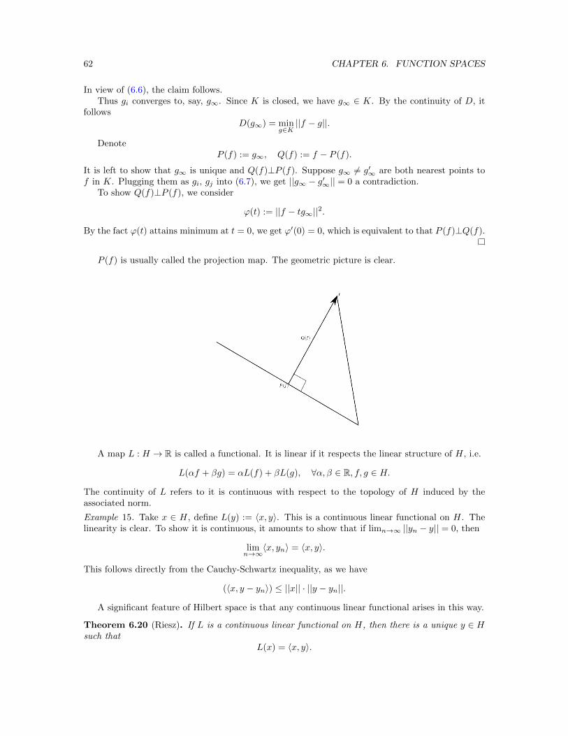
62 CHAPTER 6. FUNCTION SPACES
In view of (6.6), the claim follows.Thus gi converges to, say, g∞. Since K is closed, we have g∞ ∈ K. By the continuity of D, it
followsD(g∞) = min
g∈K||f − g||.
DenoteP (f) := g∞, Q(f) := f − P (f).
It is left to show that g∞ is unique and Q(f)⊥P (f). Suppose g∞ 6= g′∞ are both nearest points tof in K. Plugging them as gi, gj into (6.7), we get ||g∞ − g′∞|| = 0 a contradiction.
To show Q(f)⊥P (f), we consider
ϕ(t) := ||f − tg∞||2.
By the fact ϕ(t) attains minimum at t = 0, we get ϕ′(0) = 0, which is equivalent to that P (f)⊥Q(f).
P (f) is usually called the projection map. The geometric picture is clear.
A map L : H → R is called a functional. It is linear if it respects the linear structure of H, i.e.
L(αf + βg) = αL(f) + βL(g), ∀α, β ∈ R, f, g ∈ H.
The continuity of L refers to it is continuous with respect to the topology of H induced by theassociated norm.
Example 15. Take x ∈ H, define L(y) := 〈x, y〉. This is a continuous linear functional on H. Thelinearity is clear. To show it is continuous, it amounts to show that if limn→∞ ||yn − y|| = 0, then
limn→∞
〈x, yn〉 = 〈x, y〉.
This follows directly from the Cauchy-Schwartz inequality, as we have
(〈x, y − yn〉) ≤ ||x|| · ||y − yn||.
A significant feature of Hilbert space is that any continuous linear functional arises in this way.
Theorem 6.20 (Riesz). If L is a continuous linear functional on H, then there is a unique y ∈ Hsuch that
L(x) = 〈x, y〉.

6.2. HILBERT SPACE: L2 SPACES 63
Proof. If L(x) ≡ 0, then y = 0 furnishes the requirement. Otherwise, let
K = {x : L(x) = 0}.
Linearity of L implies K is a subspace and continuity shows that K is closed. Hence there existsz ∈ K⊥, with ||z|| = 1. Put
u = L(x)z − L(z)x.
Direct computation shows that L(u) = 0, thus u⊥z. We get
L(x) = L(x)||z||2 = L(z)〈x, z〉, ∀x ∈ H.
Set y = L(z)z, we get the desired y, such that
L(x) = 〈x, y〉.
Uniqueness of such y is easy. Suppose there are y and y′ such that
〈x, y〉 = 〈x, y′〉, ∀x ∈ H.
Therefore 〈x, y − y′〉 = 0, ∀x. Set x = y − y′, it follows that y = y′.

64 CHAPTER 6. FUNCTION SPACES
���PPP
dÐv´2019cSGÆÏ¢C¼ê�§ùÂ"�²��§7kéõ)Ø$�êÆ�Ø"3da��þÓƧ¦��/»ú7«0®²�·�Ø�?�"��§ùÂ�Äåé�§Ý5gü Ó1§¦�´�u�Æ�MIÂ�ÇÚ¥I�ÆEâ�Æ
�����Ç" k��ÆÏ·�Ó�?�¢C¼ê§�±²~�6�§SNÚ�Æ%�"¦����ÆngÚ�{�·éõéu"Ó�¦�)�ØN§ �ÆÏe5Ò/¤�°SN���*�ùÂ"²~k<`/¢C¼êÆ�H0§·�@´�óufhÆ)"ª,§ÐÆöN´��«°|
�E��~/òÑ0§�ù/�Ä�0¤Ø:´m"¦���3 L²nØuС��«���²§·�I[±/�ÿb��%Øy0�° §÷XÿÝ!�ÿ¼ê!È©!�©ù�Ì�c?"�Xn)��\§ �ÒúúÑ�§ýnªòwy"ùL§�ù7&�§��¥y3·�¡c�´V��È©nØù�4w�õ"±c3ÆÏ(å�§�h�Äoó��§�²���dÚ¤e¡��f"y�¹e5§Æ
Öö�W"
��ܺI+ä§�ê�\σ�ê¯pϦZzݧüN��ÚFatou��찪إ§�È��A�??�ε��<9-§y�©Û©þ´
65
![Side-Channel Analysis of Weierstrass and Koblitz Curve ... · Side-Channel Analysis of Weierstrass and Koblitz Curve ... (e.g., power consumption [27], ... modern smartphone processors](https://img.pdfslide.us/doc/110x75/5b14d71a7f8b9a8f548c4f03/side-channel-analysis-of-weierstrass-and-koblitz-curve-side-channel-analysis.jpg)


![Approximation results regarding the multiple-output ... · class of continuous functions, using the Stone-Weierstrass theorem (cf. [27]). Also via the Stone-Weierstrass theorem, [28]](https://img.pdfslide.us/doc/110x75/5f18768c209d69574d6fe9a6/approximation-results-regarding-the-multiple-output-class-of-continuous-functions.jpg)