Introduction to R

Lecturer: Zhao Jianhua

Department of StatisticsYunnan University of Finance and Economics

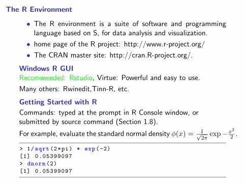
Outline

Introduction to R1.2 The R Environment1.3 Getting Started with R1.4 Using the R Online Help System1.5 Functions1.6 Arrays, Data Frames, and Lists1.7 Workspace and Files1.8 Using Scripts1.9 Using Packages1.10 Graphics

The R Environment

• The R environment is a suite of software and programminglanguage based on S, for data analysis and visualization.

• home page of the R project: http://www.r-project.org/

• The CRAN master site: http://cran.R-project.org/.

Windows R GUIRecommended: Rstudio, Virtue: Powerful and easy to use.

Many others: Rwinedit,Tinn-R, etc.

Getting Started with R

Commands: typed at the prompt in R Console window, orsubmitted by source command (Section 1.8).

For example, evaluate the standard normal density φ(x) = 1√2π

exp−x2

2 .

> 1/sqrt(2*pi) * exp(-2)

[1] 0.05399097

> dnorm (2)

[1] 0.05399097

Getting Started with R

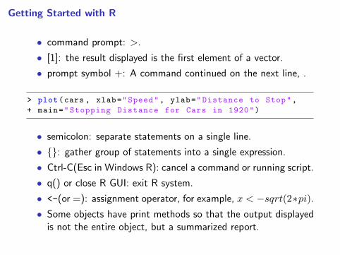
• command prompt: >.

• [1]: the result displayed is the first element of a vector.

• prompt symbol +: A command continued on the next line, .

> plot(cars , xlab="Speed", ylab="Distance to Stop",

+ main="Stopping Distance for Cars in 1920")

• semicolon: separate statements on a single line.

• {}: gather group of statements into a single expression.

• Ctrl-C(Esc in Windows R): cancel a command or running script.

• q() or close R GUI: exit R system.

• <-(or =): assignment operator, for example, x < −sqrt(2∗pi).• Some objects have print methods so that the output displayed

is not the entire object, but a summarized report.

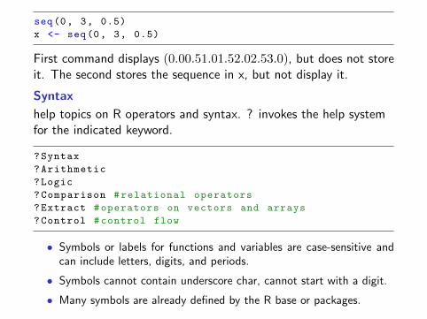
seq(0, 3, 0.5)

x <- seq(0, 3, 0.5)

First command displays (0.00.51.01.52.02.53.0), but does not storeit. The second stores the sequence in x, but not display it.

Syntax

help topics on R operators and syntax. ? invokes the help systemfor the indicated keyword.

?Syntax

?Arithmetic

?Logic

?Comparison #relational operators

?Extract #operators on vectors and arrays

?Control #control flow

• Symbols or labels for functions and variables are case-sensitive andcan include letters, digits, and periods.

• Symbols cannot contain underscore char, cannot start with a digit.

• Many symbols are already defined by the R base or packages.

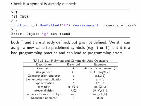
Check if a symbol is already defined:

> T

[1] TRUE

> t

function (x) UseMethod("t") <environment: namespace:base >

> g

Error: Object "g" not found

both T and t are already defined, but g is not defined. We still canassign a new value to predefined symbols (e.g. t or T), but it is abad programming practice and can lead to programming errors.

TABLE 1.1: R Syntax and Commonly Used OperatorsDescription R symbol ExampleComment # #this is a comment}

Assignment <- x <- log2(2)

Concatenation operator c c(3,2,2)Elementwise multiplication * a * b

Exponentiation ^ 2^1.5

x mod y x %% y 25 %% 3

Integer division %/% 25 %\/% 3

Sequence from a to b by h seq seq(a,b,h)Sequence operator : 0:20

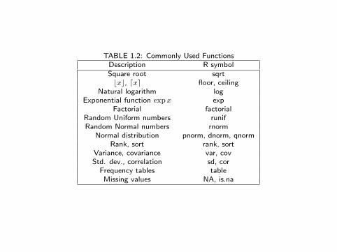
TABLE 1.2: Commonly Used FunctionsDescription R symbolSquare root sqrtbxc, dxe floor, ceiling

Natural logarithm logExponential function expx exp

Factorial factorialRandom Uniform numbers runifRandom Normal numbers rnorm

Normal distribution pnorm, dnorm, qnormRank, sort rank, sort

Variance, covariance var, covStd. dev., correlation sd, cor

Frequency tables tableMissing values NA, is.na

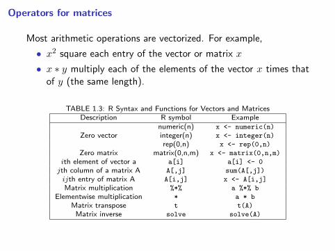
Operators for matrices

Most arithmetic operations are vectorized. For example,

• x2 square each entry of the vector or matrix x

• x ∗ y multiply each of the elements of the vector x times thatof y (the same length).

TABLE 1.3: R Syntax and Functions for Vectors and MatricesDescription R symbol Example

Zero vectornumeric(n) x <- numeric(n)

integer(n) x <- integer(n)

rep(0,n) x <- rep(0,n)

Zero matrix matrix(0,n,m) x <- matrix(0,n,m)

ith element of vector a a[i] a[i] <- 0

jth column of a matrix A A[,j] sum(A[,j])

ijth entry of matrix A A[i,j] x <- A[i,j]

Matrix multiplication %*% a %*% b

Elementwise multiplication * a * b

Matrix transpose t t(A)

Matrix inverse solve solve(A)

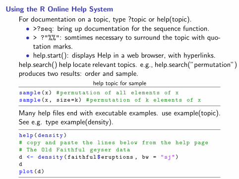
Using the R Online Help System

For documentation on a topic, type ?topic or help(topic).

• >?seq: bring up documentation for the sequence function.• > ?"%%": somtimes necessary to surround the topic with quo-

tation marks.• help.start(): displays Help in a web browser, with hyperlinks.

help.search() help locate relevant topics. e.g., help.search(”permutation”)produces two results: order and sample.

help topic for sample

sample(x) #permutation of all elements of x

sample(x, size=k) #permutation of k elements of x

Many help files end with executable examples. use example(topic).See e.g. type example(density).

help(density)

# copy and paste the lines below from the help page

# The Old Faithful geyser data

d <- density(faithful$eruptions , bw = "sj")

d

plot(d)

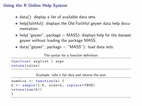
Using the R Online Help System

• data(): display a list of available data sets.

• help(faithful): displays the Old Faithful geyser data help docu-mentation

• help(“geyser”, package = MASS): displays help for the datasetgeyser without loading the package MASS.

• data(“geyser”, package = ”MASS”): load data sets.

The syntax for a function definition:

function( arglist ) expr

return(value)

Example: rolls n fair dice and returns the sum

sumdice <- function(n) {

k <- sample (1:6, size=n, replace=TRUE)

return(sum(k))

}

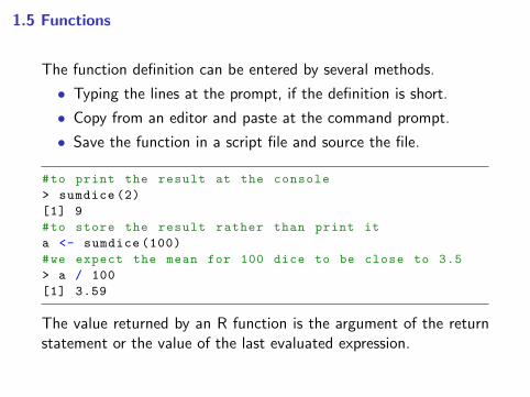
1.5 Functions

The function definition can be entered by several methods.

• Typing the lines at the prompt, if the definition is short.

• Copy from an editor and paste at the command prompt.

• Save the function in a script file and source the file.

#to print the result at the console

> sumdice (2)

[1] 9

#to store the result rather than print it

a <- sumdice (100)

#we expect the mean for 100 dice to be close to 3.5

> a / 100

[1] 3.59

The value returned by an R function is the argument of the returnstatement or the value of the last evaluated expression.

The sumdice function could be written as

sumdice <- function(n)

sum(sample (1:6, size=n, replace=TRUE))

Functions can have default argument values, e.g., sumdice can begeneralized to roll s-sided dice, but keep the default as 6-sided.

sumdice <- function(n, sides = 6) {

if (sides < 1) return (0)

k <- sample (1:sides , size=n, replace=TRUE)

return(sum(k))

}

> sumdice (5) #default 6 sides

[1] 12

> sumdice(n=5, sides =4) #4 sides

[1] 14

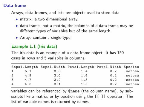
Data frame

Arrays, data frames, and lists are objects used to store data

• matrix: a two dimensional array.

• data frame: not a matrix, the columns of a data frame may bedifferent types of variables but of the same length.

• Array: contain a single type.

Example 1.1 (Iris data)

The iris data is an example of a data frame object. It has 150cases in rows and 5 variables in columns.

Sepal.Length Sepal.Width Petal.Length Petal.Width Species

1 5.1 3.5 1.4 0.2 setosa

2 4.9 3.0 1.4 0.2 setosa

3 4.7 3.2 1.3 0.2 setosa

4 4.6 3.1 1.5 0.2 setosa

variables can be referenced by $name (the column name), by sub-scripts like a matrix, or by position using the [[ ]] operator. Thelist of variable names is returned by names.

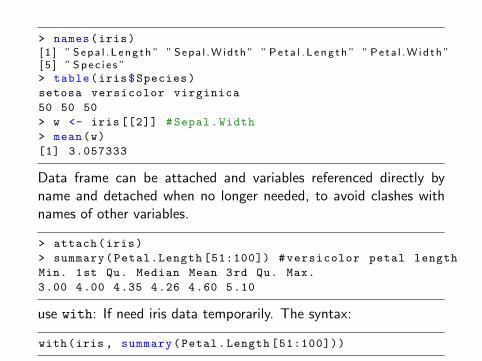
> names(iris)[ 1 ] ” S e p a l . L e n g t h ” ” S e p a l . W i d t h ” ” P e t a l . L e n g t h ” ” P e t a l . W i d t h ”[ 5 ] ” S p e c i e s ”

> table(iris$Species)setosa versicolor virginica

50 50 50

> w <- iris [[2]] #Sepal.Width

> mean(w)

[1] 3.057333

Data frame can be attached and variables referenced directly byname and detached when no longer needed, to avoid clashes withnames of other variables.

> attach(iris)

> summary(Petal.Length [51:100]) #versicolor petal length

Min. 1st Qu. Median Mean 3rd Qu. Max.

3.00 4.00 4.35 4.26 4.60 5.10

use with: If need iris data temporarily. The syntax:

with(iris , summary(Petal.Length [51:100]))

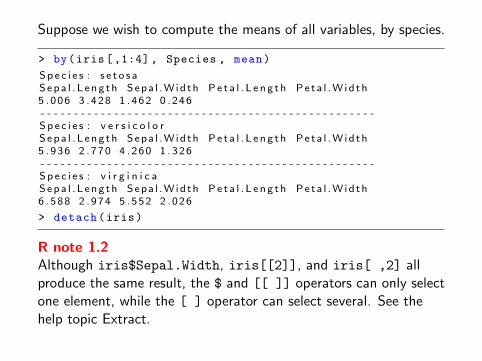
Suppose we wish to compute the means of all variables, by species.

> by(iris[,1:4], Species , mean)

S p e c i e s : s e t o s aS e p a l . L e n g t h S e p a l . W i d t h P e t a l . L e n g t h P e t a l . W i d t h5 . 0 0 6 3 . 4 2 8 1 . 4 6 2 0 . 2 4 6- - - - - - - - - - - - - - - - - - - - - - - - - - - - - - - - - - - - - - - - - - - - - - - - - -S p e c i e s : v e r s i c o l o rS e p a l . L e n g t h S e p a l . W i d t h P e t a l . L e n g t h P e t a l . W i d t h5 . 9 3 6 2 . 7 7 0 4 . 2 6 0 1 . 3 2 6- - - - - - - - - - - - - - - - - - - - - - - - - - - - - - - - - - - - - - - - - - - - - - - - - -S p e c i e s : v i r g i n i c aS e p a l . L e n g t h S e p a l . W i d t h P e t a l . L e n g t h P e t a l . W i d t h6 . 5 8 8 2 . 9 7 4 5 . 5 5 2 2 . 0 2 6

> detach(iris)

R note 1.2Although iris$Sepal.Width, iris[[2]], and iris[ ,2] allproduce the same result, the $ and [[ ]] operators can only selectone element, while the [ ] operator can select several. See thehelp topic Extract.

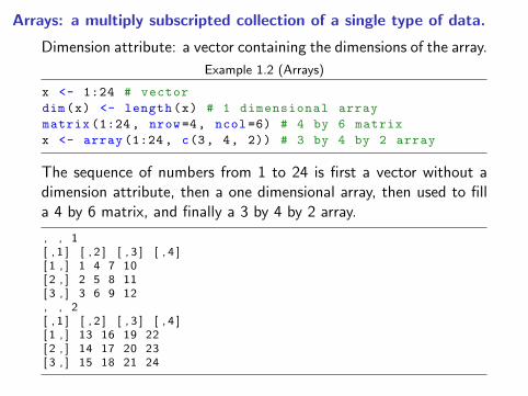
Arrays: a multiply subscripted collection of a single type of data.

Dimension attribute: a vector containing the dimensions of the array.

Example 1.2 (Arrays)

x <- 1:24 # vector

dim(x) <- length(x) # 1 dimensional array

matrix (1:24, nrow=4, ncol =6) # 4 by 6 matrix

x <- array (1:24 , c(3, 4, 2)) # 3 by 4 by 2 array

The sequence of numbers from 1 to 24 is first a vector without adimension attribute, then a one dimensional array, then used to filla 4 by 6 matrix, and finally a 3 by 4 by 2 array.

, , 1[ , 1 ] [ , 2 ] [ , 3 ] [ , 4 ][ 1 , ] 1 4 7 10[ 2 , ] 2 5 8 11[ 3 , ] 3 6 9 12, , 2[ , 1 ] [ , 2 ] [ , 3 ] [ , 4 ][ 1 , ] 13 16 19 22[ 2 , ] 14 17 20 23[ 3 , ] 15 18 21 24

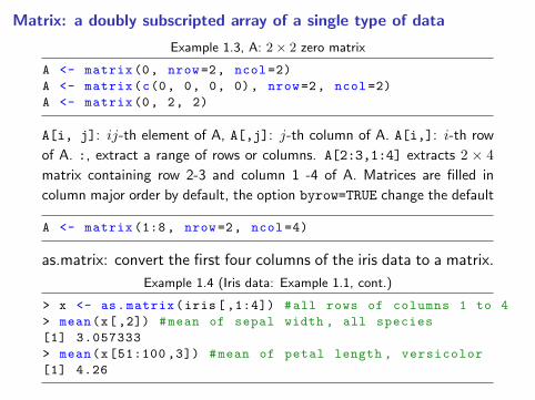
Matrix: a doubly subscripted array of a single type of data

Example 1.3, A: 2× 2 zero matrix

A <- matrix(0, nrow=2, ncol =2)

A <- matrix(c(0, 0, 0, 0), nrow=2, ncol =2)

A <- matrix(0, 2, 2)

A[i, j]: ij-th element of A, A[,j]: j-th column of A. A[i,]: i-th row

of A. :, extract a range of rows or columns. A[2:3,1:4] extracts 2 × 4

matrix containing row 2-3 and column 1 -4 of A. Matrices are filled in

column major order by default, the option byrow=TRUE change the default

A <- matrix (1:8, nrow=2, ncol =4)

as.matrix: convert the first four columns of the iris data to a matrix.

Example 1.4 (Iris data: Example 1.1, cont.)

> x <- as.matrix(iris [ ,1:4]) #all rows of columns 1 to 4

> mean(x[,2]) #mean of sepal width , all species

[1] 3.057333

> mean(x[51:100 ,3]) #mean of petal length , versicolor

[1] 4.26

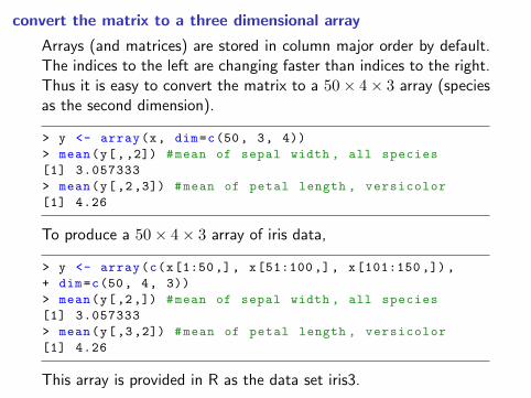
convert the matrix to a three dimensional array

Arrays (and matrices) are stored in column major order by default.The indices to the left are changing faster than indices to the right.Thus it is easy to convert the matrix to a 50× 4× 3 array (speciesas the second dimension).

> y <- array(x, dim=c(50, 3, 4))

> mean(y[,,2]) #mean of sepal width , all species

[1] 3.057333

> mean(y[,2,3]) #mean of petal length , versicolor

[1] 4.26

To produce a 50× 4× 3 array of iris data,

> y <- array(c(x[1:50,], x[51:100 ,] , x[101:150 ,]) ,

+ dim=c(50, 4, 3))

> mean(y[,2,]) #mean of sepal width , all species

[1] 3.057333

> mean(y[,3,2]) #mean of petal length , versicolor

[1] 4.26

This array is provided in R as the data set iris3.

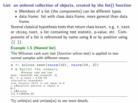
List: an ordered collection of objects, created by the list() function

• Members of a list (the components) can be different types.• data frame: list with class data.frame, more general than data

frame.

Several classical hypothesis tests that return class htest. e.g. t.testor chisq.test, a list containing test statistic, p-value, etc. Com-ponents of a list is referenced by name using $ or by position using[[ ]].

Example 1.5 (Named list)

The Wilcoxon rank sum test (function wilcox.test) is applied to twonormal samples with different means.

w <- wilcox.test(rnorm (10), rnorm(10, 2))

> w #print the summaryWilcoxon rank sum t e s t

data : rnorm ( 1 0 ) and rnorm ( 1 0 , 2)W = 2 , p - v a l u e = 4 .33e -05a l t e r n a t i v e h y p o t h e s i s :t r u e l o c a t i o n s h i f t i s not e q u a l to 0> w $ s t a t i s t i c #s t o r e d i n o b j e c t wW 2> w$p . v a l u e[ 1 ] 4 .330035e -05

Try unlist(w) and unclass(w) to see more details.

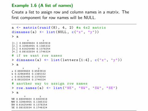
Example 1.6 (A list of names)

Create a list to assign row and column names in a matrix. Thefirst component for row names will be NULL.

a <- matrix(runif(8), 4, 2) #a 4x2 matrix

dimnames(a) <- list(NULL , c("x", "y"))

> ax y

[ 1 , ] 0 .88009604 0 .6583918[ 2 , ] 0 .32964955 0 .1385332[ 3 , ] 0 .61625490 0 .1378254[ 4 , ] 0 .08102034 0 .1746324

# if we want row names

> dimnames(a) <- list(letters [1:4], c("x", "y"))

> ax y

a 0 .88009604 0 .6583918b 0 .32964955 0 .1385332c 0 .61625490 0 .1378254d 0 .08102034 0 .1746324

# another way to assign row names

> row.names(a) <- list("NE", "NW", "SW", "SE")

> ax y

NE 0 .88009604 0 .6583918NW 0 .32964955 0 .1385332SW 0 .61625490 0 .1378254SE 0 .08102034 0 .1746324

Workspace and Files

The workspace in R contains data and other objects. User definedobjects created in a session will persist until R is closed. If theworkspace is saved before quitting R, the objects created during thesession will be saved.

• ls: display the names of objects in the current workspace.• rm or remove: remove objects from the workspace.• rm(list = ls()): remove the entire list of objects.

Recommend to check what is stored in the workspace, and removeunneeded objects.

• bad practice: save functions in the workspace• better idea: save functions in scripts and data in files. Their

collections can be documented in packages (Section 1.8-1.9).

The Working Directory

Create a folder or directory with a short path name to store yourscripts and data sets.

• getwd and setwd: get or set the current working directory.

• setwd(”/Rfiles”): set the working directory to /Rfiles

Reading Data from External Files

• scan: read univariate data from an external file.

• read.tablemany options to support different file formats

Download data at http://www.stat.ncsu.edu/sas/sicl/data/.

forearm <- scan("/Rfiles/forearm.dat") #a vector

x <- read.table("/Rfiles/irises.dat") #a data frame

> dim(x)

[1] 50 12

#get the fourth variable in the data frame

x <- read.table("/Rfiles/irises.dat")[[4]] #a vector

#read and coerce to matrix

x <- as.matrix(read.table("/Rfiles/irises.dat"))

read.table contains documentation for read.csv and read.delim, forreading comma-separated-values (.csv) files and text files with otherdelimiters. See Appendix B.3.4 for an example with .csv format.

R note 1.3By default, read.table will convert character variables to factors.Set as.is = TRUE to prevent this conversion.

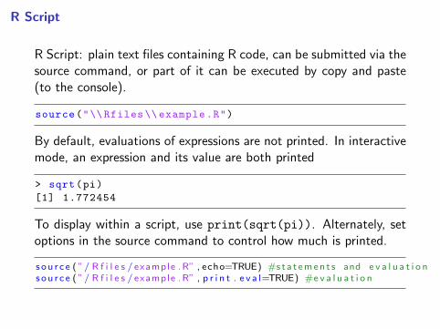
R Script

R Script: plain text files containing R code, can be submitted via thesource command, or part of it can be executed by copy and paste(to the console).

source("\\ Rfiles \\ example.R")

By default, evaluations of expressions are not printed. In interactivemode, an expression and its value are both printed

> sqrt(pi)

[1] 1.772454

To display within a script, use print(sqrt(pi)). Alternately, setoptions in the source command to control how much is printed.

s o u r c e ( ”/ R f i l e s / example . R” , echo=TRUE) #s t a t e m e n t s and e v a l u a t i o ns o u r c e ( ”/ R f i l e s / example . R” , p r i n t . e v a l=TRUE) #e v a l u a t i o n

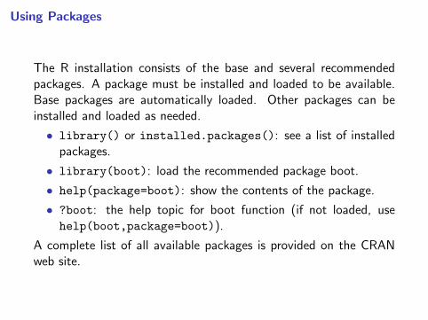
Using Packages

The R installation consists of the base and several recommendedpackages. A package must be installed and loaded to be available.Base packages are automatically loaded. Other packages can beinstalled and loaded as needed.

• library() or installed.packages(): see a list of installedpackages.

• library(boot): load the recommended package boot.

• help(package=boot): show the contents of the package.

• ?boot: the help topic for boot function (if not loaded, usehelp(boot,package=boot)).

A complete list of all available packages is provided on the CRANweb site.

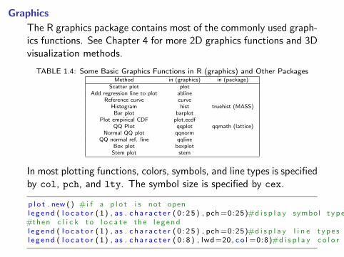
Graphics

The R graphics package contains most of the commonly used graph-ics functions. See Chapter 4 for more 2D graphics functions and 3Dvisualization methods.

TABLE 1.4: Some Basic Graphics Functions in R (graphics) and Other PackagesMethod in (graphics) in (package)

Scatter plot plotAdd regression line to plot abline

Reference curve curveHistogram hist truehist (MASS)Bar plot barplot

Plot empirical CDF plot.ecdfQQ Plot qqplot qqmath (lattice)

Normal QQ plot qqnormQQ normal ref. line qqline

Box plot boxplotStem plot stem

In most plotting functions, colors, symbols, and line types is specifiedby col, pch, and lty. The symbol size is specified by cex.

p l o t . new ( ) #i f a p l o t i s not openl e g e n d ( l o c a t o r ( 1 ) , as . c h a r a c t e r ( 0 : 2 5 ) , pch =0:25)#d i s p l a y symbol t y p e s

#then c l i c k to l o c a t e t h e l e g e n dl e g e n d ( l o c a t o r ( 1 ) , as . c h a r a c t e r ( 0 : 2 5 ) , pch =0:25)#d i s p l a y l i n e t y p e sl e g e n d ( l o c a t o r ( 1 ) , as . c h a r a c t e r ( 0 : 8 ) , lwd =20, c o l =0:8)#d i s p l a y c o l o r t y p e s

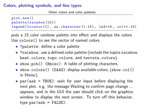
Colors, plotting symbols, and line types

Other colors and color palettes

plot.new()

palette(rainbow (15))

legend(locator (1), as.character (1:15) , lwd=15, col =1:15)

puts a 15 color rainbow palette into effect and displays the colors.Use colors() to see the vector of named colors.

• ?palette: define a color palette

• ?rainbow: use a defined color palette (include the topics rainbow,heat.colors, topo.colors, and terrain.colors).

• show.pch() (Hmisc): A table of plotting characters.

• show.colors() (DAAG): display available colors, (show.col()in Hmisc).

• par(ask = TRUE): wait for user input before displaying thenext plot. e.g. the message Waiting to confirm page change ...appears, and in the GUI the user should click on the graphicswindow to display the next screen. To turn off this behavior,type par(ask = FALSE).