Embed Size (px)
Citation preview
Introduction to R
Ariel M. Aloe1
June 6th, 2017
1The majority of these materials had been developed by “Brandon LeBeau”for his “PSQF:6250 Computer Packages for Statistical Analysis” class. All errorsare my own.
Outline
I Section I . . . Basic RI Section II . . . GraphicsI Section III . . . R ScriptI Section IV . . . Data ImportI Section V . . . Data Munging with RI Section VI . . . Joining DataI Section VII . . . Data RestructuringI Section VIII . . . Factor Variables in R

Section 1
Basic R
Background
I In an attempt to get you “doing things” in R quickly, I’veomitted a lot of discussion surrounding internal R workings.
I R is an object oriented language, this is much different thanmany other software languages.
I Within the R environment:I Everything that exist is an objectI Everything that happens is a functional callI Possible to interface with other software
I But lets start simple

R works as a calculatorR can be used as a calculator to do any type of addition,subtraction, multiplication, or division (among other things).
1 + 2 - 3
## [1] 0
5 * 7
## [1] 35
2/1
## [1] 2
sqrt(4)
## [1] 2
2^2
## [1] 4
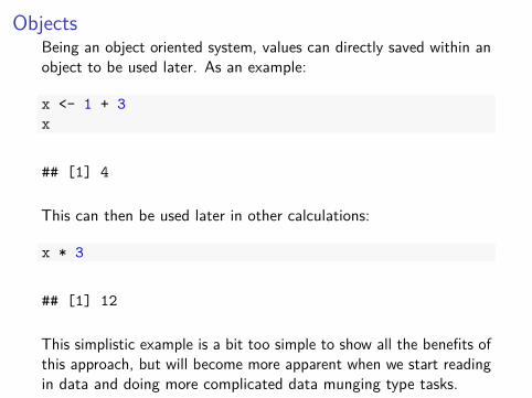
ObjectsBeing an object oriented system, values can directly saved within anobject to be used later. As an example:
x <- 1 + 3x
## [1] 4
This can then be used later in other calculations:
x * 3
## [1] 12
This simplistic example is a bit too simple to show all the benefits ofthis approach, but will become more apparent when we start readingin data and doing more complicated data munging type tasks.
Naming conventions
I This is a topic in which you will not get a single answer, butrather a different answer for everyone you ask.
I I prefer something called snake_case using underscores toseparate words in an object.
I Others use titleCase as a way to distinguish words others yetuse period.to.separate words in object names.
I The most important thing is to be consistent. Pick aconvention that works for you and stick with it through out.Avoiding this Mixed.TypeOf_conventions at all costs.
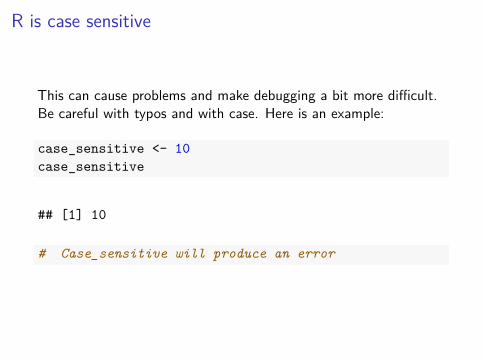
R is case sensitive
This can cause problems and make debugging a bit more difficult.Be careful with typos and with case. Here is an example:
case_sensitive <- 10case_sensitive
## [1] 10
# Case_sensitive will produce an error

FunctionsI A function consists of at least two parts, the function name
and the arguments as follows:I function_name(arg1 = num, arg2 = num).
I The arguments are always inside of parentheses, take on somevalue, and are always named. To call a function, use thefunction_name followed by parentheses with the argumentsinside the parentheses.
I For example, using the rnorm function to generate values froma random normal distribution:
set.seed(1)rnorm(n = 10, mean = 0, sd = 1)
## [1] -0.6264538 0.1836433 -0.8356286 1.5952808 0.3295078 -0.8204684## [7] 0.4874291 0.7383247 0.5757814 -0.3053884
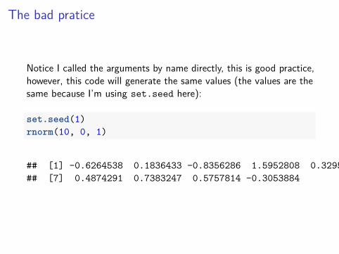
The bad pratice
Notice I called the arguments by name directly, this is good practice,however, this code will generate the same values (the values are thesame because I’m using set.seed here):
set.seed(1)rnorm(10, 0, 1)
## [1] -0.6264538 0.1836433 -0.8356286 1.5952808 0.3295078 -0.8204684## [7] 0.4874291 0.7383247 0.5757814 -0.3053884
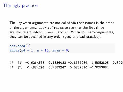
The ugly practice
The key when arguments are not called via their names is the orderof the arguments. Look at ?rnorm to see that the first threearguments are indeed n, mean, and sd. When you name arguments,they can be specified in any order (generally bad practice).
set.seed(1)rnorm(sd = 1, n = 10, mean = 0)
## [1] -0.6264538 0.1836433 -0.8356286 1.5952808 0.3295078 -0.8204684## [7] 0.4874291 0.7383247 0.5757814 -0.3053884
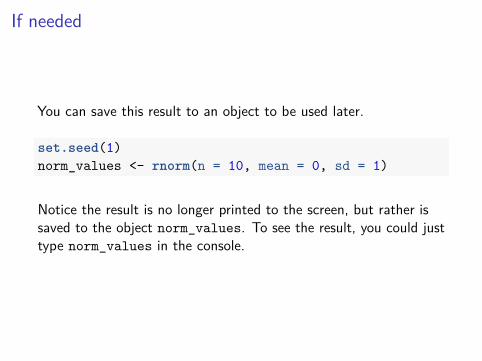
If needed
You can save this result to an object to be used later.
set.seed(1)norm_values <- rnorm(n = 10, mean = 0, sd = 1)
Notice the result is no longer printed to the screen, but rather issaved to the object norm_values. To see the result, you could justtype norm_values in the console.

ErrorsErrors are going to happen. If you encounter an error I recommenddoing the following few things first:
1. Use ?function_name to explore the details of the function.The examples at the bottom of every R help page can beespecially helpful.
2. If this does not help, copy and paste the error and search onthe internet. Chances are someone else has had this error andhas asked how to fix it. This is how I fix most errors I amunable to figure out with the R help.
3. If these two steps still do not help, you can post your error inplaces such as https://stackoverflow.com you will need toinclude the following things:
I The error message directly given from RI A reproducible example of the code. The reproducible example
is one in which helpers can run the code directly with nomodifications.
Section 2
Graphics
Background
I We are going to start by exploring graphics with R using themidwest data.
I To access this data, run the following commands:
install.packages("tidyverse")
library(tidyverse)

midwest data I
I Let’s explore these data closer, just type the name of he dataset in the console.
midwest
I This will bring up the first 10 rows of the data (hiding theadditional 8,592) rows.
I A first common step to explore our research question (e.g.,How does population density influence the percentage of thepopulation with at least a college degree?) is to plot the data.
I To do this we are going to use the R package, ggplot2, whichwas installed when running the install.packages commandabove.
I You can explore the midwest data by calling up the help file aswell with ?midwest.

midwest data II
## # A tibble: 437 × 28## PID county state area poptotal popdensity popwhite popblack## <int> <chr> <chr> <dbl> <int> <dbl> <int> <int>## 1 561 ADAMS IL 0.052 66090 1270.9615 63917 1702## 2 562 ALEXANDER IL 0.014 10626 759.0000 7054 3496## 3 563 BOND IL 0.022 14991 681.4091 14477 429## 4 564 BOONE IL 0.017 30806 1812.1176 29344 127## 5 565 BROWN IL 0.018 5836 324.2222 5264 547## 6 566 BUREAU IL 0.050 35688 713.7600 35157 50## 7 567 CALHOUN IL 0.017 5322 313.0588 5298 1## 8 568 CARROLL IL 0.027 16805 622.4074 16519 111## 9 569 CASS IL 0.024 13437 559.8750 13384 16## 10 570 CHAMPAIGN IL 0.058 173025 2983.1897 146506 16559## # ... with 427 more rows, and 20 more variables: popamerindian <int>,## # popasian <int>, popother <int>, percwhite <dbl>, percblack <dbl>,## # percamerindan <dbl>, percasian <dbl>, percother <dbl>,## # popadults <int>, perchsd <dbl>, percollege <dbl>, percprof <dbl>,## # poppovertyknown <int>, percpovertyknown <dbl>, percbelowpoverty <dbl>,## # percchildbelowpovert <dbl>, percadultpoverty <dbl>,## # percelderlypoverty <dbl>, inmetro <int>, category <chr>
midwest data III
Another useful functions to explore your data are:
I str(midwest), andI View(midwest)

Create a ggplot I
I To plot these two variables from the midwest data, we will usethe function ggplot and geom_point to add a layer of points.
I We will treat popdensity as the x variable and percollegeas the y variable.
ggplot(data = midwest) +geom_point(mapping = aes(x = popdensity,
y = percollege))
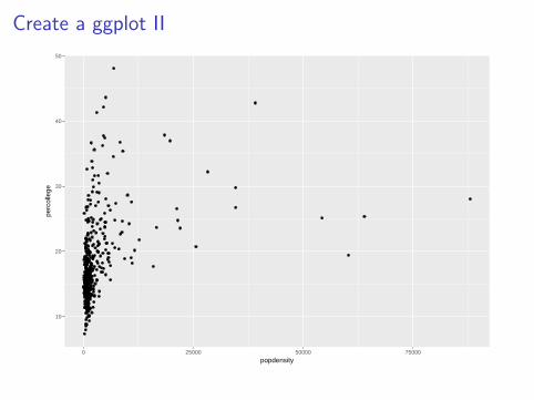
Create a ggplot II
10
20
30
40
50
0 25000 50000 75000
popdensity
perc
olle
ge
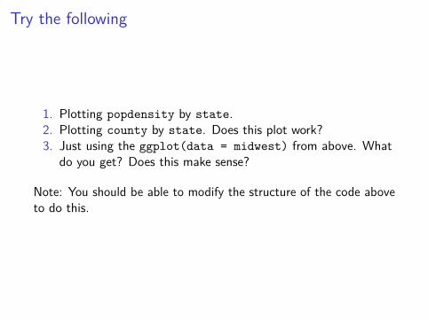
Try the following
1. Plotting popdensity by state.2. Plotting county by state. Does this plot work?3. Just using the ggplot(data = midwest) from above. What
do you get? Does this make sense?
Note: You should be able to modify the structure of the code aboveto do this.
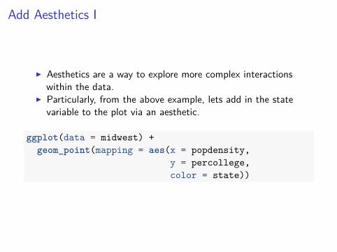
Add Aesthetics I
I Aesthetics are a way to explore more complex interactionswithin the data.
I Particularly, from the above example, lets add in the statevariable to the plot via an aesthetic.
ggplot(data = midwest) +geom_point(mapping = aes(x = popdensity,
y = percollege,color = state))

Add Aesthetics II
10
20
30
40
50
0 25000 50000 75000
popdensity
perc
olle
ge
state
IL
IN
MI
OH
WI
As you can see, we simply colored the points by the state theybelong in. Does there appear to be a trend?
Examples
1. Using the same aesthetic structure as above, instead of usingcolors, make the shape of the points different for each state.
2. Instead of color, use alpha instead. What does this do to theplot?
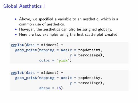
Global Aesthetics I
I Above, we specified a variable to an aesthetic, which is acommon use of aesthetics.
I However, the aesthetics can also be assigned globally.I Here are two examples using the first scatterplot created.
ggplot(data = midwest) +geom_point(mapping = aes(x = popdensity,
y = percollege),color = 'pink')
ggplot(data = midwest) +geom_point(mapping = aes(x = popdensity,
y = percollege),shape = 15)
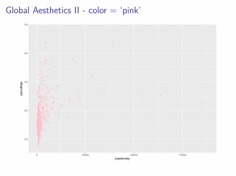
Global Aesthetics II - color = ‘pink’
10
20
30
40
50
0 25000 50000 75000
popdensity
perc
olle
ge

Global Aesthetics III - shape = 15
10
20
30
40
50
0 25000 50000 75000
popdensity
perc
olle
ge

Global Aesthetics IV
I These two plots changed the aesthetics for all of the points.I Notice, the suttle difference between the code for these plots
and that for the plot above.I The placement of the aesthetic is crucial, if it is within the
parentheses for aes() then it should be assigned a variable.I If it is outside, as in the last two examples, it will define the
aesthetic for all the data.

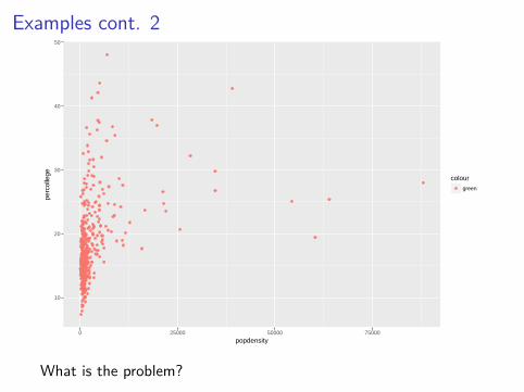
Examples
1. Try the following command: colors(). This will print a vectorof all the color names within R, try a few to find your favorites.
2. What happens if you use the following code:
ggplot(data = midwest) +geom_point(mapping = aes(x = popdensity,
y = percollege,color = 'green'))
Examples cont. 2
10
20
30
40
50
0 25000 50000 75000
popdensity
perc
olle
ge colour
green
What is the problem?
Facets I
I Instead of defining an aesthetic to change the color or shape ofpoints by a third variable, we can also plot each groups data ina single plot and combine them.
I The process is easy with ggplot2 by using facets.
ggplot(data = midwest) +geom_point(mapping = aes(x = popdensity,
y = percollege)) +facet_grid(. ~ state)
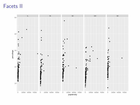
Facets IIIL IN MI OH WI
0 25000 50000 75000 0 25000 50000 75000 0 25000 50000 75000 0 25000 50000 75000 0 25000 50000 75000
10
20
30
40
50
popdensity
perc
olle
ge

Geoms I
I ggplot2 uses a grammar of graphics which makes it easy toswitch different plot types (called geoms) once you arecomfortable with the basic syntax.
I For example, how does the following plot differ from thescatterplot first generated above? What is similar?
ggplot(data = midwest) +geom_smooth(mapping = aes(x = popdensity,
y = percollege))

Geoms II
20
30
40
50
0 25000 50000 75000
popdensity
perc
olle
ge

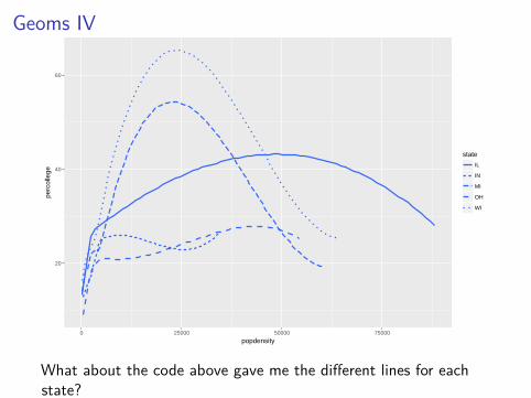
Geoms IV
We can also do this plot by states
ggplot(data = midwest) +geom_smooth(mapping = aes(x = popdensity,
y = percollege,linetype = state),
se = FALSE)
Note, I also removed the standard error shading from the plot aswell.
Geoms IV
20
40
60
0 25000 50000 75000
popdensity
perc
olle
ge
state
IL
IN
MI
OH
WI
What about the code above gave me the different lines for eachstate?

Examples
1. It is possible to combine geoms, which we will do next, but tryit first. Try to recreate this plot.
ggplot(data = midwest) +geom_point(aes(x = popdensity,
y = percollege,color = state)) +
geom_smooth(mapping = aes(x = popdensity,y = percollege,color = state),
se = FALSE)

Combining multiple geoms I
I Combining more than one geom into a single plot is relativelystraightforward, but a few considerations are important.
I Essentially to do the task, we just simply need to combine thetwo geoms we have used:
ggplot(data = midwest) +geom_point(aes(x = popdensity,
y = percollege,color = state)) +
geom_smooth(mapping = aes(x = popdensity,y = percollege,color = state),
se = FALSE)

Combining multiple geoms II
20
40
60
0 25000 50000 75000
popdensity
perc
olle
ge
state
IL
IN
MI
OH
WI

Combining multiple geoms IIII A couple points about combining geoms, first, the order
matters.I In the above example, we called geom_point first, then
geom_smooth.I When plotting these data, the points will then be plotted first
followed by the lines.I Try flipping the order of the two geoms to see how the plot
differs.I We can also simplify this code to not duplicate typing:
ggplot(data = midwest, mapping = aes(x = popdensity,y = percollege,color = state)) +
geom_point() +geom_smooth(se = FALSE)
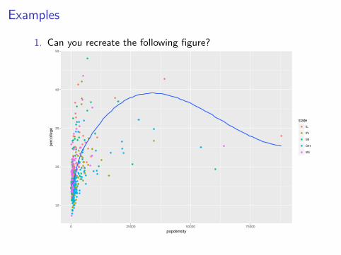
Examples
1. Can you recreate the following figure?
10
20
30
40
50
0 25000 50000 75000
popdensity
perc
olle
ge
state
IL
IN
MI
OH
WI
Other geom examples
I There are many other geoms available to use.I To see them all, visit
http://docs.ggplot2.org/current/index.html whichgives examples of all the possibilities.
I This is a handy resource that I keep going back to.
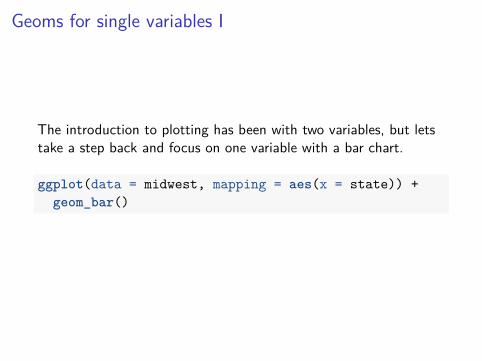
Geoms for single variables I
The introduction to plotting has been with two variables, but letstake a step back and focus on one variable with a bar chart.
ggplot(data = midwest, mapping = aes(x = state)) +geom_bar()

Geoms for single variables II
0
25
50
75
100
IL IN MI OH WI
state
coun
t
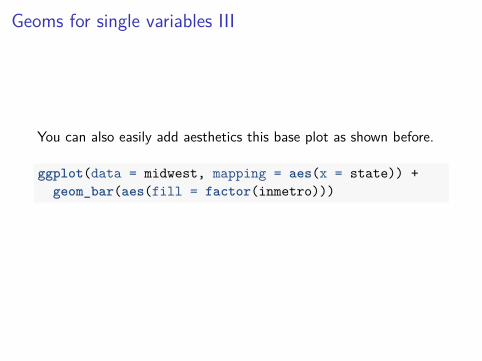
Geoms for single variables III
You can also easily add aesthetics this base plot as shown before.
ggplot(data = midwest, mapping = aes(x = state)) +geom_bar(aes(fill = factor(inmetro)))
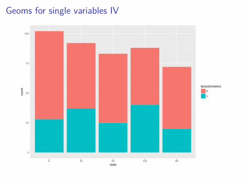
Geoms for single variables IV
0
25
50
75
100
IL IN MI OH WI
state
coun
t factor(inmetro)
0
1

Geoms for single variables V
A few additions can help interpretation of this plot:
ggplot(data = midwest, mapping = aes(x = state)) +geom_bar(aes(fill = factor(inmetro)),
position = 'fill')

Geoms for single variables VIA few additions can help interpretation of this plot:
0.00
0.25
0.50
0.75
1.00
IL IN MI OH WI
state
coun
t factor(inmetro)
0
1

Geoms for single variables VII
ggplot(data = midwest, mapping = aes(x = state)) +geom_bar(aes(fill = factor(inmetro)),
position = 'dodge')
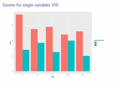
Geoms for single variables VIII
0
20
40
60
IL IN MI OH WI
state
coun
t factor(inmetro)
0
1
Geoms for single variables IX
It is also possible to do a histogram of a quantitative variable:
ggplot(data = midwest, mapping = aes(x = popdensity)) +geom_histogram()

Geoms for single variables X## `stat_bin()` using `bins = 30`. Pick better value with `binwidth`.
0
100
200
0 25000 50000 75000
popdensity
coun
t
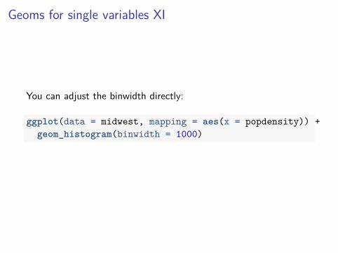
Geoms for single variables XI
You can adjust the binwidth directly:
ggplot(data = midwest, mapping = aes(x = popdensity)) +geom_histogram(binwidth = 1000)
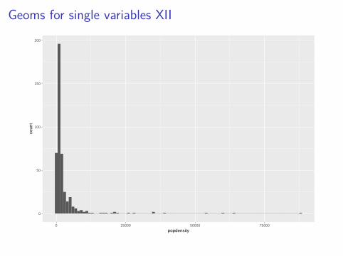
Geoms for single variables XII
0
50
100
150
200
0 25000 50000 75000
popdensity
coun
t
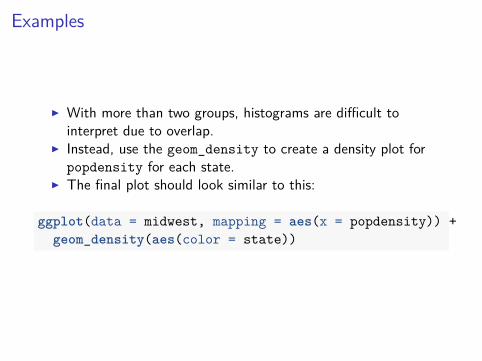
Examples
I With more than two groups, histograms are difficult tointerpret due to overlap.
I Instead, use the geom_density to create a density plot forpopdensity for each state.
I The final plot should look similar to this:
ggplot(data = midwest, mapping = aes(x = popdensity)) +geom_density(aes(color = state))
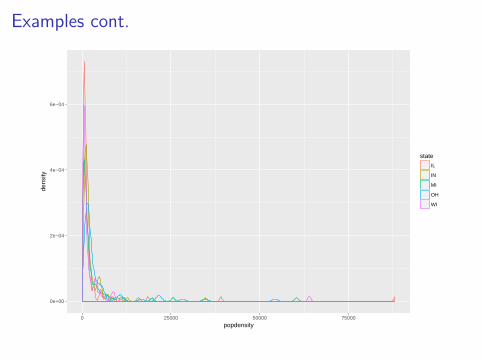
Examples cont.
0e+00
2e−04
4e−04
6e−04
0 25000 50000 75000
popdensity
dens
ity
state
IL
IN
MI
OH
WI
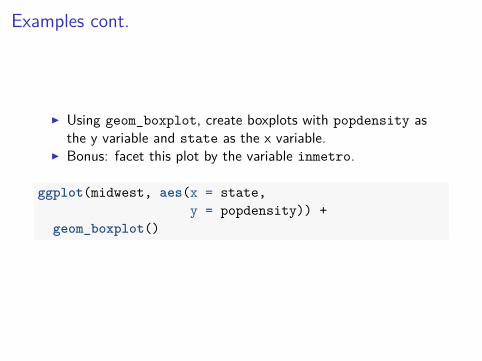
Examples cont.
I Using geom_boxplot, create boxplots with popdensity asthe y variable and state as the x variable.
I Bonus: facet this plot by the variable inmetro.
ggplot(midwest, aes(x = state,y = popdensity)) +
geom_boxplot()

Examples cont.
0
25000
50000
75000
IL IN MI OH WI
state
popd
ensi
ty

Plot CustomizationThere are many many ways to adjust the look of the plot, I willdiscuss a few that are common.
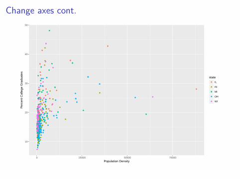
Change axes
Axes are something that are commonly altered, particularly to givethem a good name and also to alter the values shown on the axes.These are generally done with scale_x_* and scale_y_* where *is a filler based on the type of variable on the axes.
I For example:
ggplot(data = midwest, mapping = aes(x = popdensity,y = percollege,color = state)) +
geom_point() +scale_x_continuous("Population Density") +scale_y_continuous("Percent College Graduates")
Change axes cont.
10
20
30
40
50
0 25000 50000 75000
Population Density
Per
cent
Col
lege
Gra
duat
es
state
IL
IN
MI
OH
WI
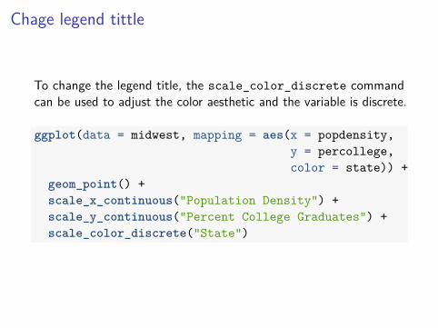
Chage legend tittle
To change the legend title, the scale_color_discrete commandcan be used to adjust the color aesthetic and the variable is discrete.
ggplot(data = midwest, mapping = aes(x = popdensity,y = percollege,color = state)) +
geom_point() +scale_x_continuous("Population Density") +scale_y_continuous("Percent College Graduates") +scale_color_discrete("State")
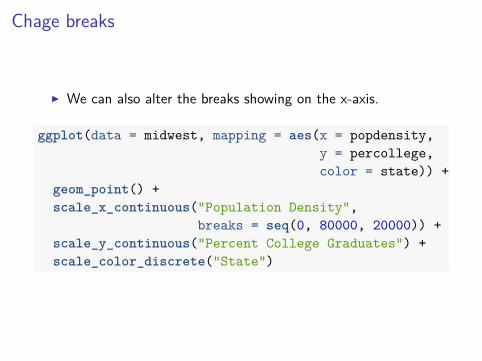
Chage breaks
I We can also alter the breaks showing on the x-axis.
ggplot(data = midwest, mapping = aes(x = popdensity,y = percollege,color = state)) +
geom_point() +scale_x_continuous("Population Density",
breaks = seq(0, 80000, 20000)) +scale_y_continuous("Percent College Graduates") +scale_color_discrete("State")

Zoom in on plot II You’ll notice that there are outliers in this scatterplot due to
larger population density values for some counties.I It may be of interest to zoom in on the plot.I The plot can be zoomed in by using the coord_cartesian
command as follows.I This can also be achieved using the xlim argument to
scale_x_continuous above, however this will cause somepoints to not be plotted.
ggplot(data = midwest, mapping = aes(x = popdensity,y = percollege,color = state)) +
geom_point() +scale_x_continuous("Population Density") +scale_y_continuous("Percent College Graduates") +scale_color_discrete("State") +coord_cartesian(xlim = c(0, 15000))

Zoom in on plot II
10
20
30
40
50
0 5000 10000 15000
Population Density
Per
cent
Col
lege
Gra
duat
es
State
IL
IN
MI
OH
WI
Section 3
R Script

R scripts I
I I want to talk very briefly about R scripts.I You may have been using these already within your workflow
for this course, but these are best practice instead of simplyrunning code in the console.
I Creating R scripts are a crucial step to ensure the data analysesare reproducible, the script will act as a log of all the thingsthat are done to the data to go from data import to anyoutputs (model results, tables, figures, etc.).

R scripts II
I To create an R script with RStudio, the short cut isCTRL/CMD + SHIFT + N.
I You can also create a new script by going to File > New File >R Script.
I Both of these commands will open up a blank script window.I In this script window, I would recommend loading any R
packages first at the top of the file.I Then proceed with the analysis.I Commands can be sent to the console using CRTL/CMD +
ENTER.I By default RStudio will run any commands that span more
than one line with a single CRTL/CMD + ENTER call.

R scripts III
I For more details about R Scripts, the R for Data Science texthas detail with screenshots in Chapter 6.
I I recommend trying to create a simple script and sending thesecommands from the script to the console to be run with R.
R scripts IV
I If you are a Linux user you can type and save your R Scriptusing, for example gedit
I Then in your terminal, you will:I set your working directory, setwd()I and read the R script, source()
Section 4
Data Import
Background
I So far we have solely used data that is already found within Rby way of packages.
I Obviously, we will want to use our own data and this involvesimporting data directly into R.
I We are going to focus on two types of data structures to readin, text files and excel files.
The following two packages will be used in this section:
library(tidyverse)# install.packages("readxl")library(readxl)
Text Files I
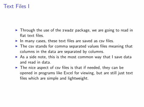
I Through the use of the readr package, we are going to read inflat text files.
I In many cases, these text files are saved as csv files.I The csv stands for comma separated values files meaning that
columns in the data are separated by columns.I As a side note, this is the most common way that I save data
and read in data.I The nice aspect of csv files is that if needed, they can be
opened in programs like Excel for viewing, but are still just textfiles which are simple and lightweight.

Text Files III To read in a csv file, we are going to use the read_csv
function from the readr package. We are going to read insome UFO data (the data can be found on ICON).
I A special note here, first, I am going to assume throughoutthat you are using RStudio projects and that the data file is ina folder called “Data”.
I If this is not the case, the path for the files listed below will notwork.
I You could use read.csv(file.choose()) to open a filebrowser.
I Or using the getwd function can help debug issues. See thelectures on R projects orhttp://r4ds.had.co.nz/workflow-projects.html foradditional information.
ufo <- read_csv("Data/ufo.csv")

Text Files III
## Parsed with column specification:## cols(## `Date / Time` = col_character(),## City = col_character(),## State = col_character(),## Shape = col_character(),## Duration = col_character(),## Summary = col_character(),## Posted = col_character()## )

Text Files IV
I Note again, similar to dplyr, when saving the data to anobject, it will not be printed.
I We can now view the first 10 rows by typing the object name.
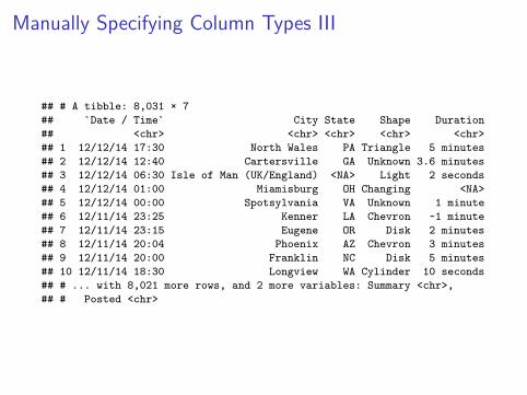
ufo

Text Files V
## # A tibble: 8,031 × 7## `Date / Time` City State Shape Duration## <chr> <chr> <chr> <chr> <chr>## 1 12/12/14 17:30 North Wales PA Triangle 5 minutes## 2 12/12/14 12:40 Cartersville GA Unknown 3.6 minutes## 3 12/12/14 06:30 Isle of Man (UK/England) <NA> Light 2 seconds## 4 12/12/14 01:00 Miamisburg OH Changing <NA>## 5 12/12/14 00:00 Spotsylvania VA Unknown 1 minute## 6 12/11/14 23:25 Kenner LA Chevron ~1 minute## 7 12/11/14 23:15 Eugene OR Disk 2 minutes## 8 12/11/14 20:04 Phoenix AZ Chevron 3 minutes## 9 12/11/14 20:00 Franklin NC Disk 5 minutes## 10 12/11/14 18:30 Longview WA Cylinder 10 seconds## # ... with 8,021 more rows, and 2 more variables: Summary <chr>,## # Posted <chr>
Text Files VI
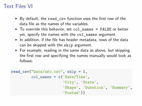
I By default, the read_csv function uses the first row of thedata file as the names of the variables.
I To override this behavior, set col_names = FALSE or betteryet, specify the names with the col_names argument.
I In addition, if the file has header metadata, rows of the datacan be skipped with the skip argument.
I For example, reading in the same data as above, but skippingthe first row and specifying the names manually would look asfollows:
read_csv("Data/ufo.csv", skip = 1,col_names = c('Date/Time',
'City', 'State','Shape', 'Duration', 'Summary','Posted'))
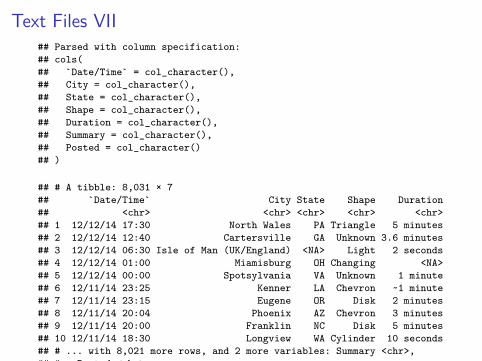
Text Files VII## Parsed with column specification:## cols(## `Date/Time` = col_character(),## City = col_character(),## State = col_character(),## Shape = col_character(),## Duration = col_character(),## Summary = col_character(),## Posted = col_character()## )
## # A tibble: 8,031 × 7## `Date/Time` City State Shape Duration## <chr> <chr> <chr> <chr> <chr>## 1 12/12/14 17:30 North Wales PA Triangle 5 minutes## 2 12/12/14 12:40 Cartersville GA Unknown 3.6 minutes## 3 12/12/14 06:30 Isle of Man (UK/England) <NA> Light 2 seconds## 4 12/12/14 01:00 Miamisburg OH Changing <NA>## 5 12/12/14 00:00 Spotsylvania VA Unknown 1 minute## 6 12/11/14 23:25 Kenner LA Chevron ~1 minute## 7 12/11/14 23:15 Eugene OR Disk 2 minutes## 8 12/11/14 20:04 Phoenix AZ Chevron 3 minutes## 9 12/11/14 20:00 Franklin NC Disk 5 minutes## 10 12/11/14 18:30 Longview WA Cylinder 10 seconds## # ... with 8,021 more rows, and 2 more variables: Summary <chr>,## # Posted <chr>

Manually Specifying Column Types I
I You may have noticed above that we just needed to give theread_csv function the path to the data file, we did not needto tell the function the types of columns.
I Instead, the function guessed the type from the first 1000 rows.I This can be useful for interactive work, but for truly
reproducible code, it is best to specify these manually.I There are two ways to specify the column types, one is verbose
and the other is simpler, but both use the argumentcol_types.
Manually Specifying Column Types II
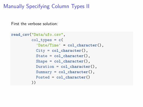
First the verbose solution:
read_csv("Data/ufo.csv",col_types = c(
'Date/Time' = col_character(),City = col_character(),State = col_character(),Shape = col_character(),Duration = col_character(),Summary = col_character(),Posted = col_character()
))
Manually Specifying Column Types III
## # A tibble: 8,031 × 7## `Date / Time` City State Shape Duration## <chr> <chr> <chr> <chr> <chr>## 1 12/12/14 17:30 North Wales PA Triangle 5 minutes## 2 12/12/14 12:40 Cartersville GA Unknown 3.6 minutes## 3 12/12/14 06:30 Isle of Man (UK/England) <NA> Light 2 seconds## 4 12/12/14 01:00 Miamisburg OH Changing <NA>## 5 12/12/14 00:00 Spotsylvania VA Unknown 1 minute## 6 12/11/14 23:25 Kenner LA Chevron ~1 minute## 7 12/11/14 23:15 Eugene OR Disk 2 minutes## 8 12/11/14 20:04 Phoenix AZ Chevron 3 minutes## 9 12/11/14 20:00 Franklin NC Disk 5 minutes## 10 12/11/14 18:30 Longview WA Cylinder 10 seconds## # ... with 8,021 more rows, and 2 more variables: Summary <chr>,## # Posted <chr>

Manually Specifying Column Types IV
As all variables are being read in as characters, there is a simpleshortcut to use.
read_csv("Data/ufo.csv",col_types = c('ccccccc'))
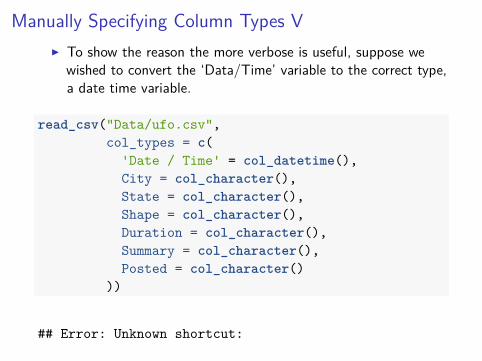
Manually Specifying Column Types VI To show the reason the more verbose is useful, suppose we
wished to convert the ‘Data/Time’ variable to the correct type,a date time variable.
read_csv("Data/ufo.csv",col_types = c(
'Date / Time' = col_datetime(),City = col_character(),State = col_character(),Shape = col_character(),Duration = col_character(),Summary = col_character(),Posted = col_character()
))
## Error: Unknown shortcut:
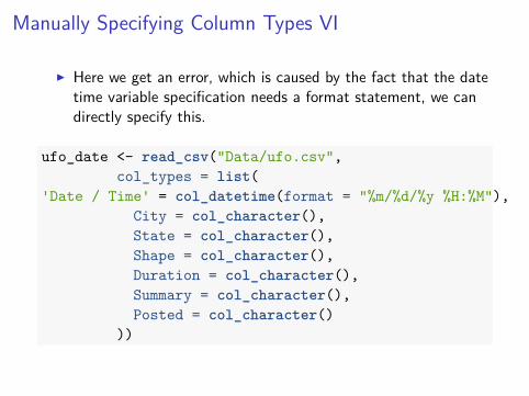
Manually Specifying Column Types VI
I Here we get an error, which is caused by the fact that the datetime variable specification needs a format statement, we candirectly specify this.
ufo_date <- read_csv("Data/ufo.csv",col_types = list(
'Date / Time' = col_datetime(format = "%m/%d/%y %H:%M"),City = col_character(),State = col_character(),Shape = col_character(),Duration = col_character(),Summary = col_character(),Posted = col_character()
))
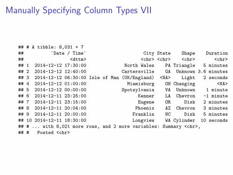
Manually Specifying Column Types VII
## # A tibble: 8,031 × 7## `Date / Time` City State Shape Duration## <dttm> <chr> <chr> <chr> <chr>## 1 2014-12-12 17:30:00 North Wales PA Triangle 5 minutes## 2 2014-12-12 12:40:00 Cartersville GA Unknown 3.6 minutes## 3 2014-12-12 06:30:00 Isle of Man (UK/England) <NA> Light 2 seconds## 4 2014-12-12 01:00:00 Miamisburg OH Changing <NA>## 5 2014-12-12 00:00:00 Spotsylvania VA Unknown 1 minute## 6 2014-12-11 23:25:00 Kenner LA Chevron ~1 minute## 7 2014-12-11 23:15:00 Eugene OR Disk 2 minutes## 8 2014-12-11 20:04:00 Phoenix AZ Chevron 3 minutes## 9 2014-12-11 20:00:00 Franklin NC Disk 5 minutes## 10 2014-12-11 18:30:00 Longview WA Cylinder 10 seconds## # ... with 8,021 more rows, and 2 more variables: Summary <chr>,## # Posted <chr>

Manually Specifying Column Types VIIII Notice even though I was careful in the column specification,
there was still issues when parsing this column as a date/timecolumn. The data is still returned, but there are issues.
I These issues can be viewed using the problems function suchas problems(ufo_date).
## # A tibble: 56 × 5## row col expected actual file## <int> <chr> <chr> <chr> <chr>## 1 119 Date / Time date like %m/%d/%y %H:%M 12/1/14 'Data/ufo.csv'## 2 194 Date / Time date like %m/%d/%y %H:%M 11/27/14 'Data/ufo.csv'## 3 236 Date / Time date like %m/%d/%y %H:%M 11/24/14 'Data/ufo.csv'## 4 407 Date / Time date like %m/%d/%y %H:%M 11/15/14 'Data/ufo.csv'## 5 665 Date / Time date like %m/%d/%y %H:%M 10/31/14 'Data/ufo.csv'## 6 797 Date / Time date like %m/%d/%y %H:%M 10/25/14 'Data/ufo.csv'## 7 946 Date / Time date like %m/%d/%y %H:%M 10/19/14 'Data/ufo.csv'## 8 1081 Date / Time date like %m/%d/%y %H:%M 10/14/14 'Data/ufo.csv'## 9 1122 Date / Time date like %m/%d/%y %H:%M 10/12/14 'Data/ufo.csv'## 10 1123 Date / Time date like %m/%d/%y %H:%M 10/12/14 'Data/ufo.csv'## # ... with 46 more rows
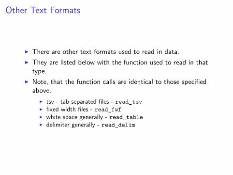
Other Text Formats
I There are other text formats used to read in data.I They are listed below with the function used to read in that
type.I Note, that the function calls are identical to those specified
above.I tsv - tab separated files - read_tsvI fixed width files - read_fwfI white space generally - read_tableI delimiter generally - read_delim

Exercises
1. Instead of specifying the path, use the functionfile.choose(). For example, read_tsv(file.choose()).What does this function use? Would you recommend this to beused in a reproducible document?
2. Run the getwd() function from the R console. What does thisfunction return?

Excel Files I
I Although I commonly use text files (e.g. csv) files, reality isthat many people still use Excel for storing of data files.
I There are good and bad aspects of this, but reading in Excelfiles may be needed.
I The readxl package is useful for this task.I Suppose we wished to read in the Excel file found on the US
Census Bureau website related to Education: https://www.census.gov/support/USACdataDownloads.html
I To do this, we can do this directly with the read_excelfunction with the data already downloaded and posted onICON.
read_excel('Data/EDU01.xls')
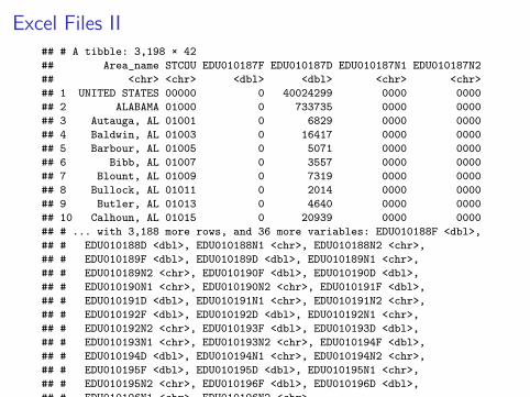
Excel Files II## # A tibble: 3,198 × 42## Area_name STCOU EDU010187F EDU010187D EDU010187N1 EDU010187N2## <chr> <chr> <dbl> <dbl> <chr> <chr>## 1 UNITED STATES 00000 0 40024299 0000 0000## 2 ALABAMA 01000 0 733735 0000 0000## 3 Autauga, AL 01001 0 6829 0000 0000## 4 Baldwin, AL 01003 0 16417 0000 0000## 5 Barbour, AL 01005 0 5071 0000 0000## 6 Bibb, AL 01007 0 3557 0000 0000## 7 Blount, AL 01009 0 7319 0000 0000## 8 Bullock, AL 01011 0 2014 0000 0000## 9 Butler, AL 01013 0 4640 0000 0000## 10 Calhoun, AL 01015 0 20939 0000 0000## # ... with 3,188 more rows, and 36 more variables: EDU010188F <dbl>,## # EDU010188D <dbl>, EDU010188N1 <chr>, EDU010188N2 <chr>,## # EDU010189F <dbl>, EDU010189D <dbl>, EDU010189N1 <chr>,## # EDU010189N2 <chr>, EDU010190F <dbl>, EDU010190D <dbl>,## # EDU010190N1 <chr>, EDU010190N2 <chr>, EDU010191F <dbl>,## # EDU010191D <dbl>, EDU010191N1 <chr>, EDU010191N2 <chr>,## # EDU010192F <dbl>, EDU010192D <dbl>, EDU010192N1 <chr>,## # EDU010192N2 <chr>, EDU010193F <dbl>, EDU010193D <dbl>,## # EDU010193N1 <chr>, EDU010193N2 <chr>, EDU010194F <dbl>,## # EDU010194D <dbl>, EDU010194N1 <chr>, EDU010194N2 <chr>,## # EDU010195F <dbl>, EDU010195D <dbl>, EDU010195N1 <chr>,## # EDU010195N2 <chr>, EDU010196F <dbl>, EDU010196D <dbl>,## # EDU010196N1 <chr>, EDU010196N2 <chr>

Excel Files III
I By default, the function will read in the first sheet and willtreat the first row as the column names.
I If you wish to read in another sheet, you can use the sheetargument.
I For example:
read_excel('Data/EDU01.xls', sheet = 2)read_excel('Data/EDU01.xls', sheet = 'EDU01B')
I If there is metadata or no column names, these can be addedin the same fashion as discussed above with the read_csvfunction.
Writing Files I
I Most of the read_* functions also come with functions thatallow you to write out files as well.
I I’m only going to cover the write_csv function, however,there are others that may be of use.
I Similarly to reading in files, the functionality is the same acrossthe write_* functions.
Writing Files II
I Suppose we created a new column with the ufo data andwished to save this data to a csv file, this can be accomplishedwith the following series of commands:
ufo_count <- ufo %>%group_by(State) %>%mutate(num_state = n())
write_csv(ufo_count, path = 'path/to/save/file.csv')
I Notice there are two arguments to the write_csv function,the first argument is the object you wish to save.
I The second is the path to the location to save the object.I You must specify path = otherwise the write_csv function
will look for that object in the R session.
Other Data Formats
I There are still other data formats, particularly from proprietarystatistical software such as Stata, SAS, or SPSS.
I To read these files in the haven function would be useful.I I leave this as an exercise for you if you have these types of files
to read into R.
Section 5
Data Munging with R
Data Munging
I Data munging (i.e. data transformations, variable creation,filtering) is a common task that is often overlooked intraditional statistics textbooks and courses.
I Data from the fivethirtyeight package is used in thissection to show the use of the dplyr verbs for data munging.
I This package can be installed with the following command:
congress_age <- read_csv("Data/congress_age.csv")

Loading packages and exploring data
I To get started with this set of notes, you will need thefollowing packages loaded:
library(readr)library(tidyverse)congress_age <- read_csv("Data/congress_age.csv")
I We are going to explore the congress_age data set in moredetail.
I Take a couple minutes to familiarize yourself with the data.
View(congress_age)?congress_age

congress_age
## # A tibble: 18,635 × 13## congress chamber bioguide firstname middlename lastname suffix## <int> <chr> <chr> <chr> <chr> <chr> <chr>## 1 80 house M000112 Joseph Jefferson Mansfield <NA>## 2 80 house D000448 Robert Lee Doughton <NA>## 3 80 house S000001 Adolph Joachim Sabath <NA>## 4 80 house E000023 Charles Aubrey Eaton <NA>## 5 80 house L000296 William <NA> Lewis <NA>## 6 80 house G000017 James A. Gallagher <NA>## 7 80 house W000265 Richard Joseph Welch <NA>## 8 80 house B000565 Sol <NA> Bloom <NA>## 9 80 house H000943 Merlin <NA> Hull <NA>## 10 80 house G000169 Charles Laceille Gifford <NA>## # ... with 18,625 more rows, and 6 more variables: birthday <date>,## # state <chr>, party <chr>, incumbent <lgl>, termstart <date>, age <dbl>

Using dplyr for data munging
I The dplyr package uses verbs for common data manipulationtasks. These include:
I filter()I arrange()I select()I mutate()I summarise()
I The great aspect of these verbs are that they all take a similardata structure, the first argument is always the data, the otherarguments are unquoted column names.
I These functions also always return a data frame in which therows are observations and the columns are variables.

Examples with filter() I
I The filter function selects rows that match a specifiedcondition(s).
I For example, suppose we wanted to select only the rows in thedata that are a part of the 80th congress.
I The following code will do this action:
filter(congress_age, congress == 80)

Examples with filter() III The filter function selects rows that match a specified
condition(s).I For example, suppose we wanted to select only the rows in the
data that are a part of the 80th congress.I The following code will do this action:
## # A tibble: 555 × 13## congress chamber bioguide firstname middlename lastname suffix## <int> <chr> <chr> <chr> <chr> <chr> <chr>## 1 80 house M000112 Joseph Jefferson Mansfield <NA>## 2 80 house D000448 Robert Lee Doughton <NA>## 3 80 house S000001 Adolph Joachim Sabath <NA>## 4 80 house E000023 Charles Aubrey Eaton <NA>## 5 80 house L000296 William <NA> Lewis <NA>## 6 80 house G000017 James A. Gallagher <NA>## 7 80 house W000265 Richard Joseph Welch <NA>## 8 80 house B000565 Sol <NA> Bloom <NA>## 9 80 house H000943 Merlin <NA> Hull <NA>## 10 80 house G000169 Charles Laceille Gifford <NA>## # ... with 545 more rows, and 6 more variables: birthday <date>,## # state <chr>, party <chr>, incumbent <lgl>, termstart <date>, age <dbl>
Examples with filter() III
I Notice from the previous slide two things, first, the functionreturned a new data frame.
I Therefore, if this subsetted data is to be saved, we need tosave it to an object, for example, as follows:
congress_80 <- filter(congress_age, congress == 80)

Examples with filter() IV
## # A tibble: 555 × 13## congress chamber bioguide firstname middlename lastname suffix## <int> <chr> <chr> <chr> <chr> <chr> <chr>## 1 80 house M000112 Joseph Jefferson Mansfield <NA>## 2 80 house D000448 Robert Lee Doughton <NA>## 3 80 house S000001 Adolph Joachim Sabath <NA>## 4 80 house E000023 Charles Aubrey Eaton <NA>## 5 80 house L000296 William <NA> Lewis <NA>## 6 80 house G000017 James A. Gallagher <NA>## 7 80 house W000265 Richard Joseph Welch <NA>## 8 80 house B000565 Sol <NA> Bloom <NA>## 9 80 house H000943 Merlin <NA> Hull <NA>## 10 80 house G000169 Charles Laceille Gifford <NA>## # ... with 545 more rows, and 6 more variables: birthday <date>,## # state <chr>, party <chr>, incumbent <lgl>, termstart <date>, age <dbl>

Example cont.
I Notice from the previous slide that equality in R is done with== not just a single =.
I The single = is used for named arguments, therefore whentesting for equality you need to be sure to use ==, this is acommon frustration and source of bugs when getting startedwith R.
I Selecting values based on a character vector are similar tonumeric values.
I For example, suppose we wanted to select only those rowspertaining to those from the senate.
I The following code will do that:
senate <- filter(congress_age, chamber == 'senate')
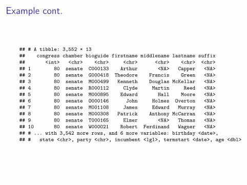
Example cont.
## # A tibble: 3,552 × 13## congress chamber bioguide firstname middlename lastname suffix## <int> <chr> <chr> <chr> <chr> <chr> <chr>## 1 80 senate C000133 Arthur <NA> Capper <NA>## 2 80 senate G000418 Theodore Francis Green <NA>## 3 80 senate M000499 Kenneth Douglas McKellar <NA>## 4 80 senate R000112 Clyde Martin Reed <NA>## 5 80 senate M000895 Edward Hall Moore <NA>## 6 80 senate O000146 John Holmes Overton <NA>## 7 80 senate M001108 James Edward Murray <NA>## 8 80 senate M000308 Patrick Anthony McCarran <NA>## 9 80 senate T000165 Elmer <NA> Thomas <NA>## 10 80 senate W000021 Robert Ferdinand Wagner <NA>## # ... with 3,542 more rows, and 6 more variables: birthday <date>,## # state <chr>, party <chr>, incumbent <lgl>, termstart <date>, age <dbl>
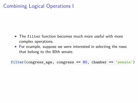
Combining Logical Operations I
I The filter function becomes much more useful with morecomplex operations.
I For example, suppose we were interested in selecting the rowsthat belong to the 80th senate.
filter(congress_age, congress == 80, chamber == 'senate')
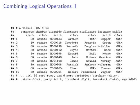
Combining Logical Operations II
## # A tibble: 102 × 13## congress chamber bioguide firstname middlename lastname suffix## <int> <chr> <chr> <chr> <chr> <chr> <chr>## 1 80 senate C000133 Arthur <NA> Capper <NA>## 2 80 senate G000418 Theodore Francis Green <NA>## 3 80 senate M000499 Kenneth Douglas McKellar <NA>## 4 80 senate R000112 Clyde Martin Reed <NA>## 5 80 senate M000895 Edward Hall Moore <NA>## 6 80 senate O000146 John Holmes Overton <NA>## 7 80 senate M001108 James Edward Murray <NA>## 8 80 senate M000308 Patrick Anthony McCarran <NA>## 9 80 senate T000165 Elmer <NA> Thomas <NA>## 10 80 senate W000021 Robert Ferdinand Wagner <NA>## # ... with 92 more rows, and 6 more variables: birthday <date>,## # state <chr>, party <chr>, incumbent <lgl>, termstart <date>, age <dbl>

Logical arguments I
I By default, the filter function uses AND when combiningmultiple arguments.
I Therefore, the above command returned only the 102 rowsbelonging to senators from the 80th congress.
I The following figure gives a list of all other possible booleanoperations.

Logical arguments II
I Note: This graphic is from the “R for Data Science” book

Logical arguments III
I Using an example of the OR operator using | to select the80th and 81st congress:
filter(congress_age, congress == 80 | congress == 81)

Logical arguments IV
I Using an example of the OR operator using | to select the80th and 81st congress:
## # A tibble: 1,112 × 13## congress chamber bioguide firstname middlename lastname suffix## <int> <chr> <chr> <chr> <chr> <chr> <chr>## 1 80 house M000112 Joseph Jefferson Mansfield <NA>## 2 80 house D000448 Robert Lee Doughton <NA>## 3 80 house S000001 Adolph Joachim Sabath <NA>## 4 80 house E000023 Charles Aubrey Eaton <NA>## 5 80 house L000296 William <NA> Lewis <NA>## 6 80 house G000017 James A. Gallagher <NA>## 7 80 house W000265 Richard Joseph Welch <NA>## 8 80 house B000565 Sol <NA> Bloom <NA>## 9 80 house H000943 Merlin <NA> Hull <NA>## 10 80 house G000169 Charles Laceille Gifford <NA>## # ... with 1,102 more rows, and 6 more variables: birthday <date>,## # state <chr>, party <chr>, incumbent <lgl>, termstart <date>, age <dbl>

Logical arguments V
I Note that to do the OR operator, you need to name thevariable twice.
I When selecting multiple values in the same variable, a handyshortcut is %in%.
I The same command can be run with the following shorthand:handy shortcut is %in%.
I The same command can be run with the following shorthand
filter(congress_age, congress %in% c(80, 81))
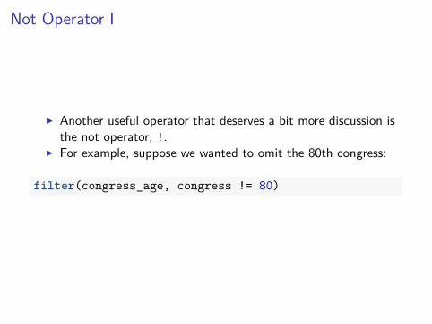
Not Operator I
I Another useful operator that deserves a bit more discussion isthe not operator, !.
I For example, suppose we wanted to omit the 80th congress:
filter(congress_age, congress != 80)

Not Operator II
## # A tibble: 18,080 × 13## congress chamber bioguide firstname middlename lastname suffix## <int> <chr> <chr> <chr> <chr> <chr> <chr>## 1 81 house D000448 Robert Lee Doughton <NA>## 2 81 house S000001 Adolph Joachim Sabath <NA>## 3 81 house E000023 Charles Aubrey Eaton <NA>## 4 81 house W000265 Richard Joseph Welch <NA>## 5 81 house B000565 Sol <NA> Bloom <NA>## 6 81 house H000943 Merlin <NA> Hull <NA>## 7 81 house B000545 Schuyler Otis Bland <NA>## 8 81 house K000138 John Hosea Kerr <NA>## 9 81 house C000932 Robert <NA> Crosser <NA>## 10 81 house K000039 John <NA> Kee <NA>## # ... with 18,070 more rows, and 6 more variables: birthday <date>,## # state <chr>, party <chr>, incumbent <lgl>, termstart <date>, age <dbl>

Not Operator III
It is also possible to do not with an AND operator as follows:
filter(congress_age, congress == 80 & !chamber == 'senate')
Exercises
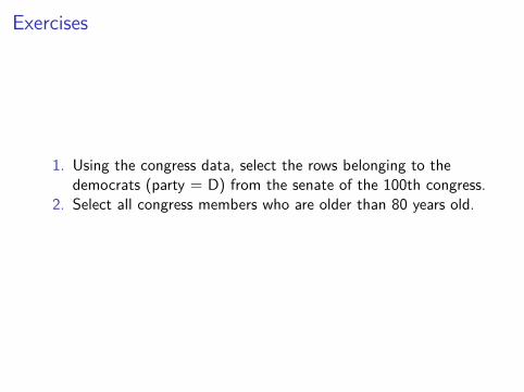
1. Using the congress data, select the rows belonging to thedemocrats (party = D) from the senate of the 100th congress.
2. Select all congress members who are older than 80 years old.

Note on Missing Data
I Missing data within R are represented with NA which stands fornot available.
I There are no missing data in the congress data, however, bydefault the filter function will not return any missing values.
I In order to select missing data, you need to use the is.nafunction.
Exercise
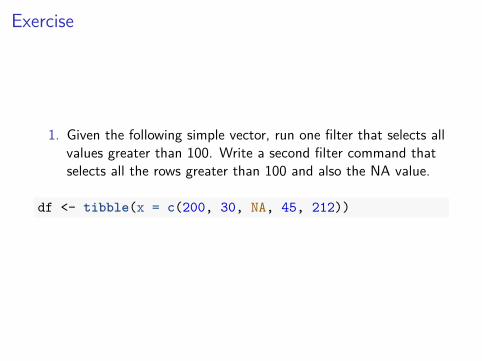
1. Given the following simple vector, run one filter that selects allvalues greater than 100. Write a second filter command thatselects all the rows greater than 100 and also the NA value.
df <- tibble(x = c(200, 30, NA, 45, 212))

Examples with arrange() I
I The arrange function is used for ordering rows in the data.I For example, suppose we wanted to order the rows in the
congress data by the state the members of congress lived in.I This can be done using the arrange function as follows:
arrange(congress_age, state)
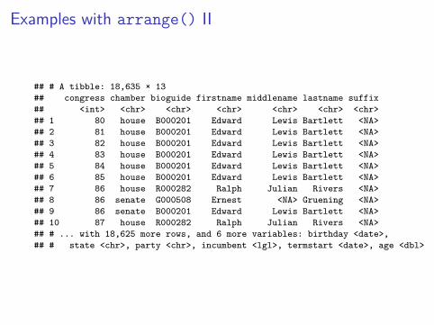
Examples with arrange() II
## # A tibble: 18,635 × 13## congress chamber bioguide firstname middlename lastname suffix## <int> <chr> <chr> <chr> <chr> <chr> <chr>## 1 80 house B000201 Edward Lewis Bartlett <NA>## 2 81 house B000201 Edward Lewis Bartlett <NA>## 3 82 house B000201 Edward Lewis Bartlett <NA>## 4 83 house B000201 Edward Lewis Bartlett <NA>## 5 84 house B000201 Edward Lewis Bartlett <NA>## 6 85 house B000201 Edward Lewis Bartlett <NA>## 7 86 house R000282 Ralph Julian Rivers <NA>## 8 86 senate G000508 Ernest <NA> Gruening <NA>## 9 86 senate B000201 Edward Lewis Bartlett <NA>## 10 87 house R000282 Ralph Julian Rivers <NA>## # ... with 18,625 more rows, and 6 more variables: birthday <date>,## # state <chr>, party <chr>, incumbent <lgl>, termstart <date>, age <dbl>
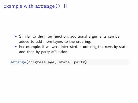
Example with arrange() III
I Similar to the filter function, additional arguments can beadded to add more layers to the ordering.
I For example, if we were interested in ordering the rows by stateand then by party affiliation.
arrange(congress_age, state, party)

Example with arrange() IV
## # A tibble: 18,635 × 13## congress chamber bioguide firstname middlename lastname suffix## <int> <chr> <chr> <chr> <chr> <chr> <chr>## 1 80 house B000201 Edward Lewis Bartlett <NA>## 2 81 house B000201 Edward Lewis Bartlett <NA>## 3 82 house B000201 Edward Lewis Bartlett <NA>## 4 83 house B000201 Edward Lewis Bartlett <NA>## 5 84 house B000201 Edward Lewis Bartlett <NA>## 6 85 house B000201 Edward Lewis Bartlett <NA>## 7 86 house R000282 Ralph Julian Rivers <NA>## 8 86 senate G000508 Ernest <NA> Gruening <NA>## 9 86 senate B000201 Edward Lewis Bartlett <NA>## 10 87 house R000282 Ralph Julian Rivers <NA>## # ... with 18,625 more rows, and 6 more variables: birthday <date>,## # state <chr>, party <chr>, incumbent <lgl>, termstart <date>, age <dbl>
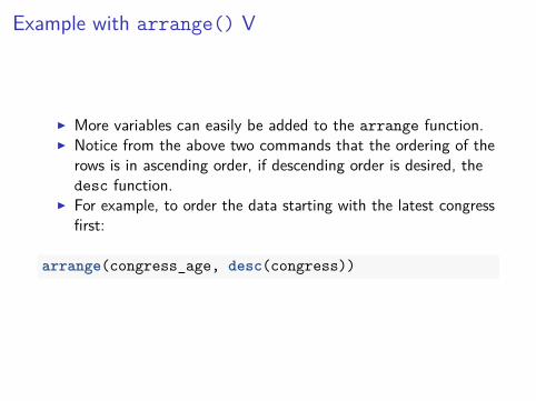
Example with arrange() V
I More variables can easily be added to the arrange function.I Notice from the above two commands that the ordering of the
rows is in ascending order, if descending order is desired, thedesc function.
I For example, to order the data starting with the latest congressfirst:
arrange(congress_age, desc(congress))

Example with arrange() VI
## # A tibble: 18,635 × 13## congress chamber bioguide firstname middlename lastname suffix## <int> <chr> <chr> <chr> <chr> <chr> <chr>## 1 113 house H000067 Ralph M. Hall <NA>## 2 113 house D000355 John D. Dingell <NA>## 3 113 house C000714 John <NA> Conyers Jr.## 4 113 house S000480 Louise McIntosh Slaughter <NA>## 5 113 house R000053 Charles B. Rangel <NA>## 6 113 house J000174 Sam Robert Johnson <NA>## 7 113 house Y000031 C. W. Bill Young <NA>## 8 113 house C000556 Howard <NA> Coble <NA>## 9 113 house L000263 Sander M. Levin <NA>## 10 113 house Y000033 Don E. Young <NA>## # ... with 18,625 more rows, and 6 more variables: birthday <date>,## # state <chr>, party <chr>, incumbent <lgl>, termstart <date>, age <dbl>
Examples with select()I
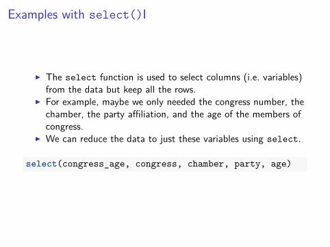
I The select function is used to select columns (i.e. variables)from the data but keep all the rows.
I For example, maybe we only needed the congress number, thechamber, the party affiliation, and the age of the members ofcongress.
I We can reduce the data to just these variables using select.
select(congress_age, congress, chamber, party, age)
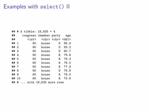
Examples with select() II
## # A tibble: 18,635 × 4## congress chamber party age## <int> <chr> <chr> <dbl>## 1 80 house D 85.9## 2 80 house D 83.2## 3 80 house D 80.7## 4 80 house R 78.8## 5 80 house R 78.3## 6 80 house R 78.0## 7 80 house R 77.9## 8 80 house D 76.8## 9 80 house R 76.0## 10 80 house R 75.8## # ... with 18,625 more rows

Examples with select() IIII Similar to the arrange functions, the variables that you wish
to keep are separated by commas and come after the dataargument.
I For more complex selection, the dplyr package has additionalfunctions that are helpful for variable selection. These include:
I starts_with()I ends_with()I contains()I matches()I num_range()
I These helper functions can be useful for selecting manyvariables that match a specific pattern.
I For example, suppose we were interested in selecting all thename variables, this can be accomplished using the containsfunction as follows:
select(congress_age, contains('name'))

Examples with select() IV
## # A tibble: 18,635 × 3## firstname middlename lastname## <chr> <chr> <chr>## 1 Joseph Jefferson Mansfield## 2 Robert Lee Doughton## 3 Adolph Joachim Sabath## 4 Charles Aubrey Eaton## 5 William <NA> Lewis## 6 James A. Gallagher## 7 Richard Joseph Welch## 8 Sol <NA> Bloom## 9 Merlin <NA> Hull## 10 Charles Laceille Gifford## # ... with 18,625 more rows
Examples with select() V
I Another useful shorthand to select multiple columns insuccession is the : operator.
I For example, suppose we wanted to select all the variablesbetween congress and birthday.
select(congress_age, congress:birthday)
Rename variables
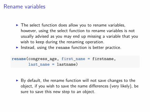
I The select function does allow you to rename variables,however, using the select function to rename variables is notusually advised as you may end up missing a variable that youwish to keep during the renaming operation.
I Instead, using the rename function is better practice.
rename(congress_age, first_name = firstname,last_name = lastname)
I By default, the rename function will not save changes to theobject, if you wish to save the name differences (very likely), besure to save this new step to an object.

Exercises
1. Using the dplyr helper functions, select all the variables thatstart with the letter ‘c’.
2. Rename the first three variables in the congress data to ‘x1’,‘x2’, ‘x3’.
3. After renaming the first three variables, use this new data(ensure you saved the previous step to an object) to selectthese three variables with the num_range function.

Examples with mutate() I
I mutate is a useful verb that allows you to add new columns tothe existing data set.
I Actions done with mutate include adding a column of means,counts, or other transformations of existing variables.
I Suppose for example, we wished to convert the party affiliationof the members of congress into a dummy (indicator) variable.
I This may be useful to more easily compute a proportion orcount for instance.
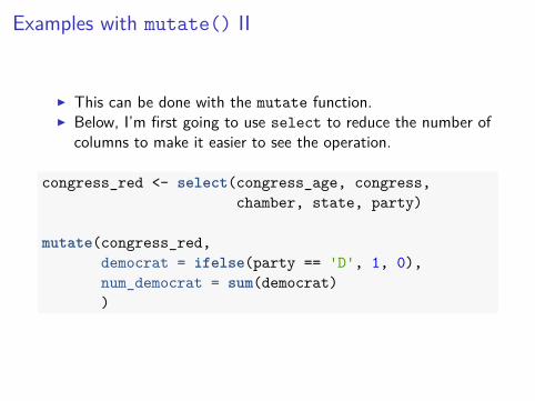
Examples with mutate() II
I This can be done with the mutate function.I Below, I’m first going to use select to reduce the number of
columns to make it easier to see the operation.
congress_red <- select(congress_age, congress,chamber, state, party)
mutate(congress_red,democrat = ifelse(party == 'D', 1, 0),num_democrat = sum(democrat))

Examples with mutate() III
## # A tibble: 18,635 × 6## congress chamber state party democrat num_democrat## <int> <chr> <chr> <chr> <dbl> <dbl>## 1 80 house TX D 1 10290## 2 80 house NC D 1 10290## 3 80 house IL D 1 10290## 4 80 house NJ R 0 10290## 5 80 house KY R 0 10290## 6 80 house PA R 0 10290## 7 80 house CA R 0 10290## 8 80 house NY D 1 10290## 9 80 house WI R 0 10290## 10 80 house MA R 0 10290## # ... with 18,625 more rows
Examples with mutate() IV
I You’ll notice that the number of rows in the data are the same(18635) as it was previously, but now the two new columnshave been added to the data.
I One converted the party affiliation to a series of 0/1 values andthe other variable counted up the number of democrats electedsince the 80th congress.
I Notice how this last variable is simply repeated for all values inthe data.
I The operation done here is not too exciting, however, we willlearn another utility later that allows us to group the data tocalculate different values for each group.

Examples with mutate() V
I Lastly, from the output above, notice that I was able toreference a variable that I created previously in the mutatecommand.
I This is unique to the dplyr package and allows you to create asingle mutate command to add many variables, even thosethat depend on prior calculations.
I Obviously, if you need to reference a calculation in anothercalculation, they need to be done in the proper order

Creation Functions
I There are many useful operators to use when creatingadditional variables.
I The R for Data Science text has many examples shown insection 5.5.1.
I In general useful operators include addition, subtraction,multiplication, division, descriptive statistics (we will talk moreabout these in week 4), ranks, logical comparisons, and manymore.
I The exercises will have you explore some of these operations inmore detail.
Exercises
1. Using the diamonds data, use ?diamonds for more informationon the data, use the mutate function to calculate the price percarat. Hint, this operation would involve standardizing theprice variable so that all are comparable at 1 carat.
2. Calculate the rank of the original price variable and the newprice variable calculated above using the min_rank function.Are there differences in the ranking of the prices? Hint, it maybe useful to test if the two ranks are equal to explore this.
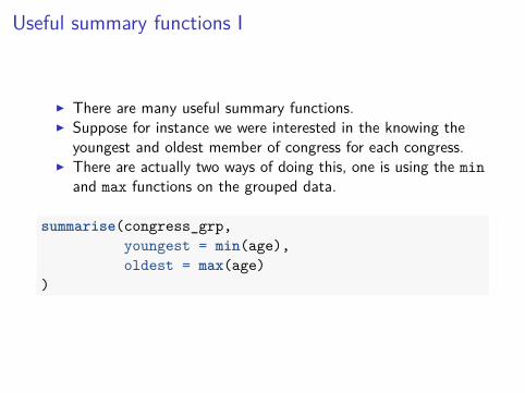
Useful summary functions I
I There are many useful summary functions.I Suppose for instance we were interested in the knowing the
youngest and oldest member of congress for each congress.I There are actually two ways of doing this, one is using the min
and max functions on the grouped data.
summarise(congress_grp,youngest = min(age),oldest = max(age)
)

Useful summary functions II
## # A tibble: 34 × 3## congress youngest oldest## <int> <dbl> <dbl>## 1 80 25.9 85.9## 2 81 27.2 85.2## 3 82 27.9 87.2## 4 83 26.7 85.3## 5 84 28.5 87.3## 6 85 30.5 89.3## 7 86 31.0 91.3## 8 87 28.9 86.0## 9 88 29.0 85.3## 10 89 25.0 87.3## # ... with 24 more rows

Exercises
1. For each congress, calculate a summary using the followingcommand: n_distinct(state). What does this value return?
2. What happens when you use a logical expression within a sumfunction call? For example, what do you get in a summarisewhen you do: sum(age > 75)?
3. What happens when you try to use sum or mean on thevariable incumbent?
Chaining together multiple operations I
I Now that you have seen all of the basic dplyr datamanipulation verbs, it is useful to chain these together tocreate more complex operations.
I In many instances, intermediate steps are not useful to us.I In these cases you can chain operations together.I Suppose we are interested in calculating the proportion of
democrats for each chamber of congress, but only since the100th congress?

Chaining together multiple operations III There are two ways to do this, the difficult to read and the
easier to read.I I first shown the difficult to read.
summarise(group_by(
mutate(filter(
congress_age, congress >= 100),democrat = ifelse(party == 'D', 1, 0)
),congress, chamber
),num_democrat = sum(democrat),total = n(),prop_democrat = num_democrat / total
)
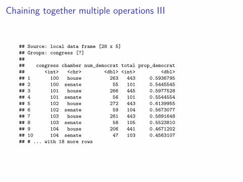
Chaining together multiple operations III
## Source: local data frame [28 x 5]## Groups: congress [?]#### congress chamber num_democrat total prop_democrat## <int> <chr> <dbl> <int> <dbl>## 1 100 house 263 443 0.5936795## 2 100 senate 55 101 0.5445545## 3 101 house 266 445 0.5977528## 4 101 senate 56 101 0.5544554## 5 102 house 272 443 0.6139955## 6 102 senate 59 104 0.5673077## 7 103 house 261 443 0.5891648## 8 103 senate 58 105 0.5523810## 9 104 house 206 441 0.4671202## 10 104 senate 47 103 0.4563107## # ... with 18 more rows
Chaining together multiple operations IV
I How difficult do you find the code above to read? This is validR code, but the first operation done is nested in the middle (itis the filter function that is run first).
I This makes for difficult code to debug and write in my opinion.I In my opinion, the better way to write code is through the pipe
operator, %>%.I The same code above can be achieved with the following much
easier to read code:

Chaining together multiple operations V
congress_age %>%filter(congress >= 100) %>%mutate(democrat = ifelse(party == 'D', 1, 0)) %>%group_by(congress, chamber) %>%summarise(
num_democrat = sum(democrat),total = n(),prop_democrat = num_democrat / total
)

Chaining together multiple operations VI
I The pipe allows for more readable code by humans andprogresses from top to bottom, left to right.
I The best word to substitute when translating the %>% codeabove is ‘then’.
I So the code above says, using the congress_age data, thenfilter, then mutate, then group_by, then summarise.
I This is much easier to read and follow the chain of commands.I I highly recommend using the pipe in your code. For more
details on what is actually happening, the R for Data Sciencebook has a good explanation in Section 5.6.1.
Exercises
1. Look at the following nested code and determine what is beingdone. Then translate this code to use the pipe operator.

Exercises cont.summarise(
group_by(mutate(
filter(diamonds,
color %in% c('D', 'E', 'F') & cut %in% c('Fair','Good','Very Good')),
f_color = ifelse(color == 'F', 1, 0),vg_cut = ifelse(cut == 'Very Good', 1, 0)),
clarity ),avg = mean(carat),sd = sd(carat),avg_p = mean(price),num = n(),summary_f_color = mean(f_color),summary_vg_cut = mean(vg_cut) )

Section 6
Joining Data
Background I
I Another common data manipulation task is to join multipledata sources into a single data file for an analysis.
I This task is most easily accomplished using a set of joinfunctions found in the dplyr package.
I In this set of notes we are going to focus on mutating joins andfiltering joins.
I There is another class of joins called set operations.I I use these much less frequently, but for those interested, see
the text in the R for Data Science bookhttp://r4ds.had.co.nz/relational-data.html.
Packages
For this section, we are going to make use of two packages:
library(tidyverse)# install.packages('Lahman')library(Lahman)

Lahman Package
I The Lahman package contains data from the Major LeagueBaseball (MLB), a professional baseball association in theUnited States.
I For this section, we are going to focus on the following threedata tables, Teams, Salaries, and Managers.
I You can print the first ten rows of the data for each tablebelow.
TeamsSalariesManagers
Inner Join I
I The most basic join is the inner join.I This join takes two tables and returns values if key variables
match in both tables.I If rows do not match on the key variables, these observations
are removed.I Suppose for example, we wanted to select the rows that
matched between the Teams and Salaries data.I This would be useful for example if we wished to calculate the
average salary of the players for each team for every year.
Inner Join II
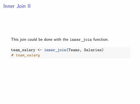
This join could be done with the inner_join function.
team_salary <- inner_join(Teams, Salaries)# team_salary
Inner Join III
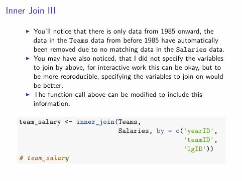
I You’ll notice that there is only data from 1985 onward, thedata in the Teams data from before 1985 have automaticallybeen removed due to no matching data in the Salaries data.
I You may have also noticed, that I did not specify the variablesto join by above, for interactive work this can be okay, but tobe more reproducible, specifying the variables to join on wouldbe better.
I The function call above can be modified to include thisinformation.
team_salary <- inner_join(Teams,Salaries, by = c('yearID',
'teamID','lgID'))
# team_salary

dplyr verbs and then plot I
We could then use other dplyr verbs to calculate the average salaryfor every team by year and plot these.
team_salary %>%group_by(yearID, teamID) %>%summarise(avg_salary = mean(salary, na.rm = TRUE)) %>%ggplot(aes(x = yearID, y = avg_salary)) +geom_line(size = 1) +facet_wrap(~teamID)

dplyr verbs and then plot II
SLN TBA TEX TOR WAS
OAK PHI PIT SDN SEA SFN
MIL MIN ML4 MON NYA NYN
FLO HOU KCA LAA LAN MIA
CHA CHN CIN CLE COL DET
ANA ARI ATL BAL BOS CAL
1990 2000 2010 1990 2000 2010 1990 2000 2010 1990 2000 2010 1990 2000 2010
1990 2000 2010
0e+002e+064e+066e+068e+06
0e+002e+064e+066e+068e+06
0e+002e+064e+066e+068e+06
0e+002e+064e+066e+068e+06
0e+002e+064e+066e+068e+06
0e+002e+064e+066e+068e+06
yearID
avg_
sala
ry

Diagram I
Below is a diagram of the inner join found in the R for Data Sciencetext:
Left Join I
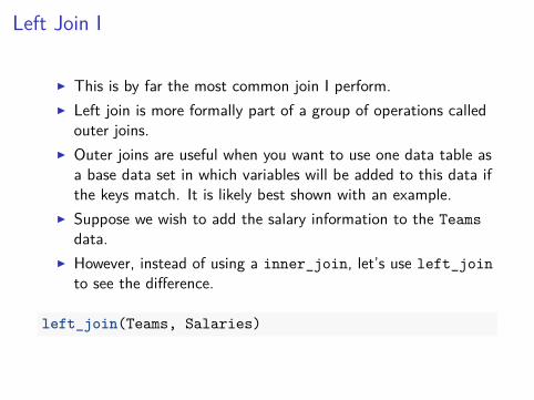
I This is by far the most common join I perform.I Left join is more formally part of a group of operations called
outer joins.I Outer joins are useful when you want to use one data table as
a base data set in which variables will be added to this data ifthe keys match. It is likely best shown with an example.
I Suppose we wish to add the salary information to the Teamsdata.
I However, instead of using a inner_join, let’s use left_jointo see the difference.
left_join(Teams, Salaries)

Left Join II
I The first thing to notice is that now there are years in theyearID variable from before 1985, this was not the case in theabove data joined using inner_join.
I If you scroll over to explore variables to the right, there aremissing values for the salary variable.
I What left_join does when it doesn’t find a match in thetable is to produce NA values, so all records within the joineddata will be NA before 1985.
I This is the major difference between outer joins and inner joins.I Outer joins will preserve data in the keyed data that do not
match and NA values are returned for non-matching values.I For inner joins, any keys that do not match are removed.
Right Join
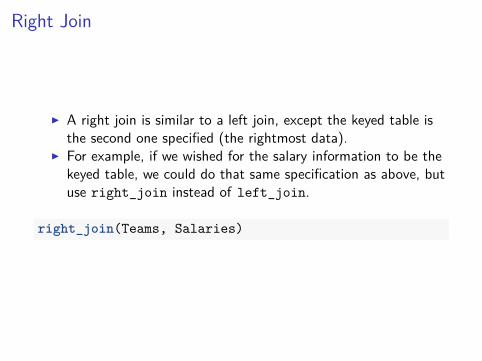
I A right join is similar to a left join, except the keyed table isthe second one specified (the rightmost data).
I For example, if we wished for the salary information to be thekeyed table, we could do that same specification as above, butuse right_join instead of left_join.
right_join(Teams, Salaries)
Full Join
I Full join is the last type of outer join and this will return allvalues from both tables and NAs will be given for those keysthat do not match.
I For example,
full_join(Teams, Salaries)

Diagram IIBelow is a diagram of the inner join found in the R for Data Sciencetext:

Filtering Joins I
I We can also use filtering joins, however, these are useful toconnect summary data back to the original rows in the data.
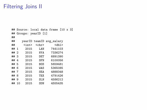
I For example, using the team_salary data created above, let’sselect only the top 10 teams in terms of average salary fromthe year 2015.
top_salary_15 <- team_salary %>%group_by(yearID, teamID) %>%summarise(avg_salary = mean(salary, na.rm = TRUE)) %>%filter(yearID == 2015) %>%arrange(desc(avg_salary)) %>%head(10)
top_salary_15
Filtering Joins II
## Source: local data frame [10 x 3]## Groups: yearID [1]#### yearID teamID avg_salary## <int> <chr> <dbl>## 1 2015 LAN 7441103## 2 2015 NYA 7336274## 3 2015 DET 6891390## 4 2015 SFN 6100056## 5 2015 BOS 5659481## 6 2015 WAS 5365085## 7 2015 SEA 4888348## 8 2015 TEX 4791426## 9 2015 SLN 4586212## 10 2015 SDN 4555435
Exercises
1. Using the Teams and Managers data, join the two tables andonly keep the matching observations in both tables. Note, youmay need to specify the column names directly you wish to joinby. What happens to the columns that have the same namesbut are not keys?
2. Using the same data tables from #1, add all the Managersvariables to the Teams data while retaining all the rows for theTeams data.

Section 7
Data Restructuring

Background II Data restructuring is often a useful tool to have.I By data restructuring, I mean transforming data from long to
wide format or vice versa.I For the most part, long format is much easier to use when
plotting and computing summary statistics. A related topic,called tidy data, can be read about in more detail here:http://www.jstatsoft.org/v59/i10/paper.
I The data we are going to use for this section of notes is called“LongitudinalEx.csv” and can be found on ICON.
I The packages needed for this section and loading the data file,assuming it is found in the “Data” folder and the workingdirectory is set to the root of the project, are as follows:
library(tidyverse)long_data <- read_csv("Data/LongitudinalEx.csv")

Long/Stacked Data I
I The data read in above is in a format that is commonlyreferred to as long or stacked data.
I These data do not have one individual per row, instead eachrow is a individual by wave combination and are stacked foreach individual (notice the three rows for id = 4).
I The variables in this case each have there own column in thedata and all of them are time varying (change for each wave ofdata within an individual).
I This is also an example of “tidy data” from the paper linked toabove, where each row is a unique observation (id, wave pair),variables are in the columns, and each cell of the data is avalue.

Long/Stacked Data II## Parsed with column specification:## cols(## id = col_integer(),## wave = col_integer(),## agegrp = col_double(),## age = col_double(),## piat = col_integer(),## agegrp.c = col_integer(),## age.c = col_double()## )
## # A tibble: 27 × 7## id wave agegrp age piat agegrp.c age.c## <int> <int> <dbl> <dbl> <int> <int> <dbl>## 1 4 1 6.5 6.000000 18 0 -0.5000000## 2 4 2 8.5 8.500000 31 2 2.0000000## 3 4 3 10.5 10.666667 50 4 4.1666667## 4 27 1 6.5 6.250000 19 0 -0.2500000## 5 27 2 8.5 9.166667 36 2 2.6666667## 6 27 3 10.5 10.916667 57 4 4.4166667## 7 31 1 6.5 6.333333 18 0 -0.1666667## 8 31 2 8.5 8.833333 31 2 2.3333333## 9 31 3 10.5 10.916667 51 4 4.4166667## 10 33 1 6.5 6.333333 18 0 -0.1666667## # ... with 17 more rows
Extra Long Data I
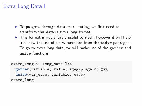
I To progress through data restructuring, we first need totransform this data is extra long format.
I This format is not entirely useful by itself, however it will helpuse show the use of a few functions from the tidyr package. -To go to extra long data, we will make use of the gather andunite functions.
extra_long <- long_data %>%gather(variable, value, agegrp:age.c) %>%unite(var_wave, variable, wave)
extra_long
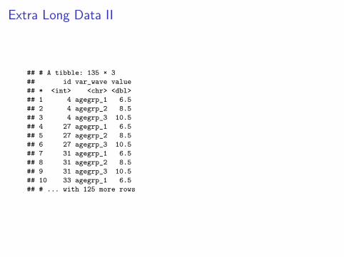
Extra Long Data II
## # A tibble: 135 × 3## id var_wave value## * <int> <chr> <dbl>## 1 4 agegrp_1 6.5## 2 4 agegrp_2 8.5## 3 4 agegrp_3 10.5## 4 27 agegrp_1 6.5## 5 27 agegrp_2 8.5## 6 27 agegrp_3 10.5## 7 31 agegrp_1 6.5## 8 31 agegrp_2 8.5## 9 31 agegrp_3 10.5## 10 33 agegrp_1 6.5## # ... with 125 more rows

Extra Long Data III
I Now there are only three columns in the data and that thereare now 135 rows in data.
I This extra long data format gathered all of the variables intotwo columns, one that identify the variable and wave and theother that simply lists the value.
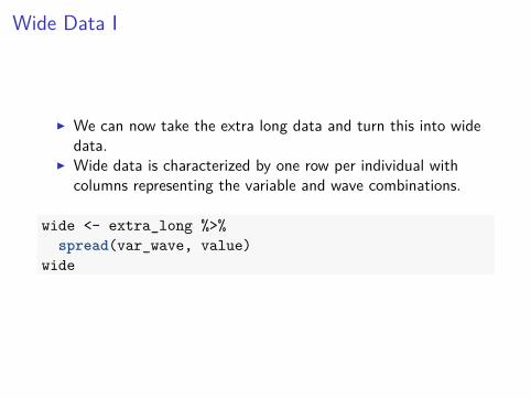
Wide Data I
I We can now take the extra long data and turn this into widedata.
I Wide data is characterized by one row per individual withcolumns representing the variable and wave combinations.
wide <- extra_long %>%spread(var_wave, value)
wide

Wide Data II
## # A tibble: 9 × 16## id age.c_1 age.c_2 age.c_3 age_1 age_2 age_3 agegrp.c_1## * <int> <dbl> <dbl> <dbl> <dbl> <dbl> <dbl> <dbl>## 1 4 -0.5000000 2.000000 4.166667 6.000000 8.500000 10.66667 0## 2 27 -0.2500000 2.666667 4.416667 6.250000 9.166667 10.91667 0## 3 31 -0.1666667 2.333333 4.416667 6.333333 8.833333 10.91667 0## 4 33 -0.1666667 2.416667 4.250000 6.333333 8.916667 10.75000 0## 5 41 -0.1666667 2.250000 4.333333 6.333333 8.750000 10.83333 0## 6 49 0.0000000 2.250000 4.166667 6.500000 8.750000 10.66667 0## 7 69 0.1666667 2.666667 4.833333 6.666667 9.166667 11.33333 0## 8 77 0.3333333 1.583333 3.500000 6.833333 8.083333 10.00000 0## 9 87 0.4166667 2.916667 5.000000 6.916667 9.416667 11.50000 0## # ... with 8 more variables: agegrp.c_2 <dbl>, agegrp.c_3 <dbl>,## # agegrp_1 <dbl>, agegrp_2 <dbl>, agegrp_3 <dbl>, piat_1 <dbl>,## # piat_2 <dbl>, piat_3 <dbl>
Wide Data III
I You’ll notice from the data above, there are now only 9 rows,but now 16 columns in the data.
I Each variable except for id now also has a number appended toit to represent the wave of the data.
I This data structure is common, particularly for users of SPSSor Excel for data entry or processing.
I Unfortunately, when working with data in R (and in general),data in wide format is often difficult to work with.
I Therefore it is common to need to restructure the data fromwide to long format.

Back to Long Format I
I Fortunately, we can use the same functions as we used above,but now in inverse to get from wide to long format.
wide %>%gather(variable, value, -id) %>%separate(variable, into = c('variable', 'wave'),
sep = "_") %>%arrange(id, wave) %>%spread(variable, value)
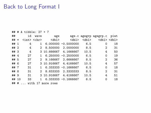
Back to Long Format I
## # A tibble: 27 × 7## id wave age age.c agegrp agegrp.c piat## * <int> <chr> <dbl> <dbl> <dbl> <dbl> <dbl>## 1 4 1 6.000000 -0.5000000 6.5 0 18## 2 4 2 8.500000 2.0000000 8.5 2 31## 3 4 3 10.666667 4.1666667 10.5 4 50## 4 27 1 6.250000 -0.2500000 6.5 0 19## 5 27 2 9.166667 2.6666667 8.5 2 36## 6 27 3 10.916667 4.4166667 10.5 4 57## 7 31 1 6.333333 -0.1666667 6.5 0 18## 8 31 2 8.833333 2.3333333 8.5 2 31## 9 31 3 10.916667 4.4166667 10.5 4 51## 10 33 1 6.333333 -0.1666667 6.5 0 18## # ... with 17 more rows

Back to Long Format I
I In addition, below is the code that would go directly from longto wide.
long_data %>%gather(variable, value, agegrp:age.c) %>%unite(var_wave, variable, wave) %>%spread(var_wave, value)

Exercises
1. Using the following data generation code, convert these data tolong format.
set.seed(10)messy <- data.frame(
id = 1:4,trt = sample(rep(c('control', 'treatment'), each = 2)),work.T1 = runif(4),home.T1 = runif(4),work.T2 = runif(4),home.T2 = runif(4)
)
2. Once successfully converted to long format, convert back towide format.

Section 8
Factor Variables in R
Background I
I When using the readr or readxl packages to read in data,the variables are read in as character strings instead of factors.
I However, there are situations when factors are useful.I This set of notes will make use of the following three packages:
library(tidyverse)library(forcats)
Uses for Factors I
To see a few of the benefits of a factor, assume we have a variablethat represents the levels of a survey question with five possibleresponses and we only saw three of those response categories.
resp <- c('Disagree', 'Agree', 'Neutral')
Uses for Factors II
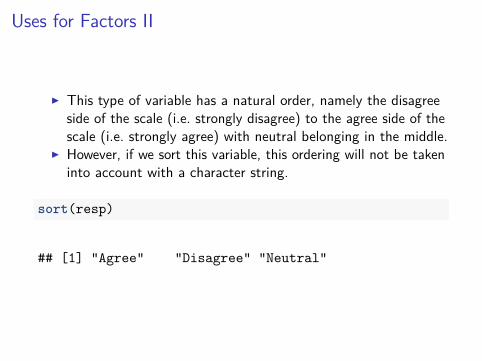
I This type of variable has a natural order, namely the disagreeside of the scale (i.e. strongly disagree) to the agree side of thescale (i.e. strongly agree) with neutral belonging in the middle.
I However, if we sort this variable, this ordering will not be takeninto account with a character string.
sort(resp)
## [1] "Agree" "Disagree" "Neutral"
Uses for Factors III
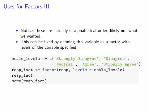
I Notice, these are actually in alphabetical order, likely not whatwe wanted.
I This can be fixed by defining this variable as a factor withlevels of the variable specified.
scale_levels <- c('Strongly Disagree', 'Disagree','Neutral', 'Agree', 'Strongly Agree')
resp_fact <- factor(resp, levels = scale_levels)resp_factsort(resp_fact)
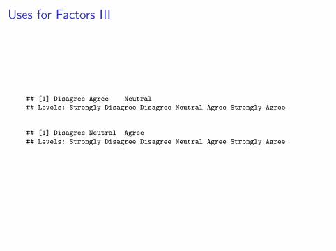
Uses for Factors III
## [1] Disagree Agree Neutral## Levels: Strongly Disagree Disagree Neutral Agree Strongly Agree
## [1] Disagree Neutral Agree## Levels: Strongly Disagree Disagree Neutral Agree Strongly Agree

Uses for Factors IV
I Another benefit, if values that are not found in the levels of thefactor variable, these will be replaced with NAs.
I For example,
knitr::asis_output("\\scriptsize") # ignore this line
factor(c('disagree', 'Agree', 'Strongly Agree'),levels = scale_levels)
## [1] <NA> Agree Strongly Agree## Levels: Strongly Disagree Disagree Neutral Agree Strongly Agree
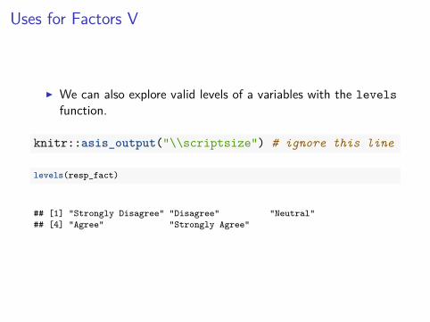
Uses for Factors V
I We can also explore valid levels of a variables with the levelsfunction.
knitr::asis_output("\\scriptsize") # ignore this line
levels(resp_fact)
## [1] "Strongly Disagree" "Disagree" "Neutral"## [4] "Agree" "Strongly Agree"

Exercises
1. How are factors stored internally by R? To explore this, use thestr function on a factor variable and see what it looks like?
2. To further this idea from #1, what happens when you do eachof the following commands? Why is this happening?
as.numeric(resp)as.numeric(resp_fact)


![sms.math.nus.edu.sg...By (3), we have the relation cosA cosB cosC = 4~2 [5 2-(2R + r)]. Therefore ABC is an acute-angled triangle, a right-angled triangle, or an obtuse-angled triangle](https://img.pdfslide.us/doc/110x75/5eb289e00225fb34fd7f64c2/smsmathnusedusg-by-3-we-have-the-relation-cosa-cosb-cosc-42-5-2-2r.jpg)